Designing Experiments Informed
by Observational Studies
Abstract
The increasing availability of passively observed data has yielded a growing methodological interest in “data fusion.” These methods involve merging data from observational and experimental sources to draw causal conclusions – and they typically require a precarious tradeoff between the unknown bias in the observational dataset and the often-large variance in the experimental dataset. We propose an alternative approach to leveraging observational data, which avoids this tradeoff: rather than using observational data for inference, we use it to design a more efficient experiment.
We consider the case of a stratified experiment with a binary outcome, and suppose pilot estimates for the stratum potential outcome variances can be obtained from the observational study. We extend results from Zhao et al., 2019 in order to generate confidence sets for these variances, while accounting for the possibility of unmeasured confounding. Then, we pose the experimental design problem as one of regret minimization, subject to the constraints imposed by our confidence sets. We show that this problem can be converted into a convex minimization and solved using conventional methods. Lastly, we demonstrate the practical utility of our methods using data from the Women’s Health Initiative.
1 Introduction
The past half-century of causal inference research has engendered a healthy skepticism toward observational data (Imbens and Rubin, 2015). In observational data sets, researchers do not control whether or not each individual receives a treatment of interest. Hence, they cannot be certain that treated individuals and untreated individuals are otherwise comparable.
This challenge can be overcome only if the covariates measured in the observational data are sufficiently rich to fully explain who receives the treatment and who does not. This is a fundamentally untestable assumption – and even if it holds, careful modeling is necessary to remove the selection effect. The applied literature includes myriad examples of treatments that showed promise in observational studies only to be overturned by later randomized trials (Hartman et al., 2015). One prominent case, the effect of hormone therapy on the health of postmenopausal women, will be discussed in this manuscript (Writing Group for the Women’s Health Initiative Investigators, 2002).
The “virtuous” counterpart to observational data is the well-designed experiment. Data from a randomized trial yield unbiased estimates of a causal effect without the need for problematic statistical assumptions. Yet experiments are frequently expensive, and, as a consequence, generally involve fewer units. Especially if one is interested in subgroup causal effects, this means experimental estimates can be imprecise.
In this paper, we discuss an approach that allows us to leverage the availability of observational data, while retaining the attractive unbiasedness properties of randomized experiments: we use the observational data not for inference, but rather to influence the design of the experiment. Our discussion will be limited to settings with binary outcomes, in which computations are tractable. We suppose the experiment has a stratified design, and seek to determine allocations of units to strata and treatment assignments.
Suppose pilot estimates of the stratum potential outcome variances are obtained from the observational study. If the outcomes are binary, we show that recent advances in sensitivity analysis from Zhao et al., 2019 can be extended to generate confidence sets for these variances, while incorporating the possibility of unmeasured confounding. Next, we pose the experimental design problem as one of regret minimization subject to the potential outcome variances lying within their confidence sets. We use a trick from von Neumann to convert the problem into a convex (though non-DCP) minimization, which can be solved using projected gradient descent. This approach can yield modest efficiency gains in the experiment, especially if there is heterogeneity in treatment effects and baseline incidence rates across strata.
The remainder of the paper proceeds as follows. Section defines our notation, assumptions, and loss function. Section gives our main results. These include the derivation of bias-aware confidence sets for the pilot variance estimates; the formulation of the design problem as a regret minimization; and the strategy to convert that problem into a computationally tractable one. We demonstrate the practical utility of our methods on data from the Women’s Health Initiative in Section . Section discusses future work and concludes.
2 Problem Set-Up
2.1 Sources of Randomness
We suppose we have access to an observational study with units in indexing set such that . We associate with each unit a pair of unseen potential outcomes ; an observed covariate vector where ; a propensity score denoting that probability of receiving treatment. We also associate with each a treatment indicator and an observed outcome defined by .
There are multiple perspectives on randomness in causal inference. In the setting of Rubin, 1974 – as in much of the early potential outcomes literature – all quantities are treated as fixed except, the treatment assignment . More modern approaches sometimes treat the potential outcomes and and covariates as random variables (VanderWeele and Robins, 2012, see e.g.). Similarly, some authors treat all of the data elements (including the treatment assignment ) as random draws from a super-population (Imbens and Rubin, 2015, see e.g.). Per the discussion in Chin, 2019, these subtleties often have little effect on the choice of estimators, but they do affect the population to which results can be generalized.
In our setting, we assume that the RCT data has not yet been collected, so it does not make sense to talk about their fixed potential outcomes. More naturally, we treat the potential outcomes and covariates as random. Thus, we view as drawn from a joint distribution . The RCT data will be denoted (with a slight abuse of notation) as for , sampled from a joint distribution . Because we are treating the potential outcomes as random variables, we can reason about their means and variances under the distribution .
2.2 Stratification and Assumptions
We will make the following assumptions about allocation to treatment.
Assumption 1 (Allocations to Treatment).
For , for . For , treatment is allocated via a simple random sample of size for .
We suppose we have a fixed stratification scheme based on the covariates . This can be derived from substantive knowledge or from applying a modern machine learning algorithm on the observational study to uncover treatment heterogeneity (Wager and Athey, 2018; Hill, 2011, e.g.). The stratification is such that there are strata and each has an associated population weight . Using the stratification on the observational study, we define indexing subsets with cardinalities to identify units in each stratum. For each stratum, define as the set of covariate values defining the stratum, such that .
Suppose we can recruit only total units for the RCT. We need to decide both the number of units recruited for each stratum, subject to the constraint , and the count of units we will assign to treatment vs. control in each stratum, such that the associated counts and sum to . Hence, our variables of interest will be .
Define and as expectations and variances under the distributions and , respectively. We will need two further assumptions.
Assumption 2 (Common Potential Outcome Means).
Conditional on the stratum, the potential outcome averages for the two populations are equal. In other words,
for all . We denote these shared quantities as and .
Assumption 3 (Common Potential Outcome Variances).
Conditional on the stratum, the potential outcome means for the two populations are equal. In other words,
for all . We denote these shared quantities as and .
2.3 Loss and Problem Statement
Given Assumption , we can define a mean effect,
for each . We can collect these values into a vector .
Denote the associated causal estimates derived from the RCT as for . We can collect these estimates into a vector . We use a weighted loss when estimating the causal effects across strata,
Our goal will be to minimize the risk, defined as an expectation of the loss over both the treatment assignments and the potential outcomes. For simplicity, we suppress the subscript and write
3 Converting to an Optimization Problem
3.1 Naïve Approach
Were known exactly, it would be straightforward to compute optimal allocations in the RCT. The optimal choice from minimizing this quantity is simply:
| (1) |
which yields a risk of
Assumption guarantees shared variance across the observational and RCT datasets. So we might be tempted to obtain pilot estimates of and from the observational study and then to plug them in to determine the allocation of units in the RCT. However, any estimate of the variances derived from the observational study should be treated with caution. Our assumptions do not preclude the possibility of unmeasured confounding, which can introduce substantial bias into the pilot estimation step. Hence, a framework that exclusively optimizes expected loss is incongruent with what we know about sources of uncertainty.
3.2 Regret Minimization
Decision theory provides an attractive framework in the form of regret minimization, originally attributed to Bell, 1982, as well as Loomes and Sugden, 1982. In this framework, a decision-maker chooses between multiple prospects, and cares not only about the received payoff but also about the foregone choice. If the foregone choice would have yielded higher payoff than the chosen one, the decision-maker experiences regret (Diecidue and Somasundaram, 2017). Decisions are made to minimize the maximum possible regret.
In our case, the decision is in how to allocate units in our RCT. One choice is an allocation informed by the observational study. The other is a “default” allocation against which we seek to compare. Denote the default values as and , where a common choice would be equal allocation, for all ; or weighted allocation for all .
Regret is defined as the difference between the risk of our chosen allocation and the default allocation,
Choosing this as our objective, we can now begin to formulate an optimization problem.
Suppose we can capture our uncertainty about via a convex constraint, indexed by a user-defined parameter ,
where . We could then obtain the regret-minimizing unit allocations as the solution to
| (2) | ||||
Defining and solving Optimization Problem will be the goal of the remainder of this paper.
3.3 Tractable Case: Binary Outcomes
To construct our confidence regions , we will extend recent sensitivity analysis results from Zhao et al., 2019.
The authors consider the case of causal estimation via stabilized inverse probability of treatment weighting (SIPW). Zhao and co-authors focus on observational studies, and consider the case where unmeasured confounding is present. To quantify this confounding, they propose a marginal sensitivity model indexed by a quantity , which bounds the odds ratio between the true treatment probability (a function of the covariates and the potential outcomes) and the treatment probability marginalized over the potential outcomes (a function of the covariates only). Their method extends the widely-used Rosenbaum sensitivity model (Rosenbaum, 1987).
The authors’ focus is on developing valid confidence intervals for the average treatment effect even when -level confounding may be present. They offer two key insights. First, they demonstrate that for any choice of , one can efficiently compute upper and lower bounds on the true potential outcome means via linear fractional programming. These bounds, referred to as the “partially identified region,” quantify the possible bias in the point estimate of the ATE. Second, the authors show that the bootstrap is valid in this setting. Hence, they propose drawing repeated bootstrap replicates; computing extrema within each replicate using their linear fractional programming approach; and then taking the relevant -level quantiles of these extrema. This procedure yields a valid -level confidence region for the ATE.
We adapt this approach to our setting in the case of binary outcomes. Note that if , then potential outcome variances can be expressed directly as a function of potential outcome means, via
As Zhao et al., 2019 provides the necessary machinery to bound mean estimates, we can exploit this relationship between the means and variances to bound variance estimates. In particular, we can show that the bootstrap is also valid if our estimand is , rather than , for and . Computing the extrema is also straightforward. Note that the function is monotonically increasing in if and monotonically decreasing in if . Hence, if we use the Zhao et al., 2019 method to solve for a partially identified region for and , we can equivalently compute such intervals for and .
Denote as the upper bound and the lower bound computed for a mean for . Denote and as the analogous quantities for variance. We apply the following logic:
- •
If , set
- •
If , set
- •
If and , set
Hence, we propose the following procedure for deriving valid confidence regions for for each choice of :
- 1.
Draw bootstrap replicates from the units .
- 2.
For each replicate:
- •
Compute for using Zhao and co-authors’ linear fractional programming approach.
- •
Determine and for using the approach described above.
- •
- 3.
Each replicate can now be represented as a rectangle in , where one axis represents the value of , and the other the value of and the vertices correspond to the extrema. Any set such that a proportion of the rectangles have all four corners included in the set will asymptotically form a valid -level confidence interval.
A full proof of the validity of this method can be found in Appendix .
Note that the final step does not specify the shape of the confidence set (it need not even be convex). For simplicity, we compute the minimum volume ellipsoid containing all vertices, then shrink the ellipsoid toward its center until only of the rectangles have all four of their vertices included. For details on constructing the ellipsoids (sometimes known as Löwner-John ellipsoids), see Boyd et al., 2004. Observe that this is by no means the smallest valid confidence set, but it is convex and easy to work with numerically.
In Figure , we demonstrate this procedure on simulated data using . We suppose there are four strata, each containing 1,000 observational units. The strata differ in their treatment probabilities with 263, 421, 564, and 739 units in each stratum, respectively. The large black dot at the center of each cluster represents the point estimate . In purple, we plot the rectangles corresponding to the extrema computed in each of 200 bootstrap replicates drawn from the data. The dashed ellipsoids represent 90% confidence sets. In the cases of strata 2 and 4, the ellipsoids extend beyond the upper bound of 0.25 in at least one direction, so we intersect the ellipsoids with the hard boundary at 0.25. The resulting final confidence sets, and , are all convex.

The objective is convex in and affine (and thus concave) in . Now, having obtained convex constraints, we can invoke Von Neumann’s minimax theorem (Von Neumann, 1928) to switch the order of the minimization and maximization. Hence, the solution to Problem is equivalent to the solution of
| subject to | |||
But the inner problem has an explicit solution, given by
Plugging this in yields the simplified problem
| (3) | ||||
Problem is concave. See Appendix for a detailed proof. The solution is non-trivial, owing to the fact that the problem is not DCP-compliant. Nonetheless, a simple projected gradient descent algorithm is guaranteed to converge under very mild conditions given the curvature (Iusem, 2003). Hence, we can efficiently solve this problem.
4 Application to the Data from the Women’s Health Initiative
4.1 Setup
To evaluate our methods in practice, we make use of data from the Women’s Health Initiative, a 1991 study of the effects of hormone therapy on postmenopausal women. The study included both a randomized controlled trial and an observational study. A total of 16,608 women were included in the trial, with half randomly selected to take 625 mg of estrogen and 2.5 mg of progestin, and the remainder receiving a placebo. A corresponding 53,054 women in the observational component of the WHI were deemed clinically comparable to women in the trial. About a third of these women were using estrogen plus progestin, while the remaining women in the observational study were not using hormone therapy (Prentice et al., 2005).
We investigate the effect of the treatment on incidence of coronary heart disease. The data is split into two non-overlapping subsets, which we term the “gold” and “silver” datasets. We estimate the probability of treatment for observational units via fitted propensity scores. The data split is the same as the one used in Rosenman et al., 2018. Details on the construction of these data elements can be found in the Appendix, Section , while further details about the WHI can be found in the Supplement, Section .
To choose our subgroups for stratification, we utilize the clinical expertise of researchers in the study’s writing group. The trial protocol highlights age as an important subgroup variable to consider (Writing Group for the Women’s Health Initiative Investigators, 1998), while subsequent work considered a patient’s history of cardiovascular disease (Roehm, 2015). We also consider Langley scatter, a measure of solar irradiance at each woman’s enrollment center, which is not plausibly related to baseline incidence or treatment effect. Langley scatter exhibits no association with the outcome in the observational control population: a Pearson’s Chi-squared test yields a p-value of 0.89. The analogous tests for age and history of cardiovascular disease have p-values below .
The age variable has three levels, corresponding to whether a woman was in her fifties, sixties, or seventies. The cardiovascular disease history variable is binary. The Langley scatter variable has five levels, corresponding to strata between 300 and 500 Langleys of irradiance. We provide brief summaries of these variables in Tables , , and in Appendix Section .
The RCT gold dataset is used to estimate “gold standard” stratum causal effects. We now suppose that the observational study is being used to design an experiment of size units. We compare the estimates from the designed pseudo-experiments against the gold standard estimates under the unweighted loss.
In the design setting, we face the additional challenge of choosing the appropriate value of . The WHI provides a very rich set of covariates, and our propensity model incorporates more than 50 variables spanning the demographic and clinical domains (see details in Appendix Section ). Hence, we will run our algorithm at values of (reflecting no residual confounding) as well as and (reflecting a modest amount).
4.2 Detailed Example: , Fine Stratification
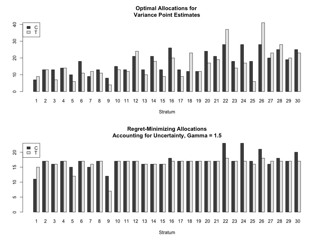
We show one example in detail, in which we choose and stratify on all three subgroup variables: age, history of cardiovascular disease, and Langley scatter. The cross-product of these variables yields 30 subgroups, which we suppose are weighted equally. We number these groups from 1 through 30.
In the top panel of Figure , we show a naïve RCT allocation based purely on the pilot estimates of the stratum potential outcome variances from the observational study. In the bottom panel, we show the regret-minimizing allocations. Visually, it is clear that we have heavily shrunk the allocations toward an equally allocated RCT, but there remain some strata where we recommend over- or under-sampling. Note, too, that the shrinkage is not purely reflective of the magnitude of the pilot estimate, since the number of observational units from each stratum and treatment status also influences the width of our confidence regions for each of the pilot estimates.
To investigate the utility of our regret-minimizing allocations, we sample pseudo-experiments of 1,000 units from the RCT silver dataset 1,000 times with replacement. We do so under three designs: equal allocation by strata; naïve allocation based on the pilot estimates; and regret-minimizing allocations. Below, we show the average loss when compared against the gold standard estimates derived from the RCT gold estimate. Results are shown in Figure . Our method yields a modest reduction in average loss (3.6%) relative to the naïve design. It also outperforms the equal design, though by a slimmer margin (1.6%). This is encouraging – especially because the design was intended to guard against worst-case loss, rather than to optimize average loss.

4.3 Performance Over Multiple Conditions
We now simulate with all possible combinations of the stratification variables. For each choice of a stratification, we select units under equal allocation, naïve allocation, and regret-minimizing allocation with and . We then compute the loss versus the “gold standard” estimates derived from the RCT gold datasets.
In Table , we summarize the loss relative to equal allocation. We see immediately that the entries are all non-positive. This makes some intuitive sense: the objective in Problem can always be set to 0 by choosing and for all ; hence, the algorithm is designed to guarantee that we cannot do worse than allocating equally. By the same token, many of the gains we see are modest, owing to the conservatism of the regret-minimizing approach. Notably, we seem to achieve the greatest gains when we are stratifying only on clinically relevant variables and using a relatively low value of . We achieve a 5-6% risk reduction at low values of in the fourth row of the table, in which we stratify on the clinically relevant age and cardiovascular disease variables. On the other hand, the algorithm quickly defaults to recommending equal allocation when variables are not clinically relevant. In the third row, in which we stratify only on the irrelevant Langley scatter variable, the starred entries correspond to cases in which the regret-minimizing allocation is equal allocation.
| Subgroup Variable(s) | Equal Alloc Loss | Loss Relative to Equal Allocation | |||
|---|---|---|---|---|---|
| Age | 0.000517 | 2.0% | |||
| CVD | 0.000498 | 2.3% | |||
| Langley | 0.000841 | 0.0% | 0.0%* | 0.0%* | 0.0%* |
| Age, CVD | 0.001541 | 5.5% | |||
| Age, Langley | 0.003417 | 1.6% | |||
| CVD, Langley | 0.002495 | 1.7% | |||
| Age, CVD, Langley | 0.008395 | 1.9% | |||
In Table , we summarize the loss relative to naïve allocation. In this case, our method can underperform a naïve allocation derived from the observational study pilot variance estimates. This can be seen most clearly in the first row of the table, in which we stratify only on the age variable. Such underperformance is a consequence of the fact that our algorithm is defensive toward underperformance when bias and variance are present in the pilot estimates. However, there are two clear trends in the results. First, when we stratify on a variable that turns out not to be clinically relevant, like Langley scatter, the naïve allocation is essentially just recommending an allocation based on noise from the data; as a result, our regret-minimizing allocations uniformly outperform naïve allocations. Second, the regret-minimizing allocations tend to outperform the naïve allocations as the number of strata grow. We significantly outperform naïve allocation in the final row, which corresponds to stratification on all three variables and a total of 30 strata.
| Subgroup Variable(s) | Naïve Alloc Loss | Loss Relative to Naïve Allocation | |||
|---|---|---|---|---|---|
| Age | 0.000501 | 1.2% | 1.2% | 1.1% | 3.2% |
| CVD | 0.000488 | 0.3% | 0.0% | 0.6% | 2.1% |
| Langley | 0.000852 | 1.1% | 1.3% | 1.3% | 1.3% |
| Age, CVD | 0.001484 | 1.8% | 1.9% | 0.1% | 1.5% |
| Age, Langley | 0.003393 | 0.9% | 0.9% | 0.0% | 0.6% |
| CVD, Langley | 0.002481 | 1.1% | 0.7% | 0.3% | 0.3% |
| Age, CVD, Langley | 0.008574 | 3.9% | 4.1% | 3.6% | 2.8% |
While these simulation results show modest performance gains, they are encouraging. A wise analyst would be extremely cautious about designing an RCT exclusively using observational study pilot estimates of stratum variances. Because such pilot estimates can have both bias and variance, relying too heavily upon them might waste resources. Our framework allows data from the observational study to be incorporated into the RCT design while guarding against the possibility of underperforming a default allocation.
5 Future Work: General Case
We briefly discuss challenges in the more general case of . In keeping with the theme of IPW estimation, we consider estimators of the form
| (4) | ||||
where are the true treatment probabilities. Such estimators are asymptotically unbiased.
Under the sensitivity model of Zhao et al., 2019, we suppose we estimate with fitted propensity scores, , defined as
In the typical setting in which we use logistic regression to estimate the propensity scores, .
We account for the possibility of -level unmeasured confounding by allowing the true probability to satisfy
Any affine transformation of our optimization variable will not change the curvature of the problem, so we redefine the problem in terms of the , an affine function of the . We define two vectors and , and analogously define vectors and . Now, we can express the equations in as quadratic fractional program, e.g.
where
We have few guarantees on the curvature of the problem: the numerators will be neither convex nor concave in the terms, , as long as the vectors and are linearly independent. The denominators will be convex in the terms. This poses a major challenge. Quadratic fractional programming problems can be solved efficiently in some special cases, but are, in general, NP-hard (Phillips, 2001).
One promising avenue for future work is to apply Dinkelbach’s method to transform the quadratic fractional problem to a series of quadratic programming problems (Dinkelbach, 1967). This will not immediately yield a solution because of the indefinite numerator, but it will allow us to make use of considerable recent work on new solution methods in quadratic programming (Park and Boyd, 2017, see e.g.).
References
- Akaike, (1974) Akaike, H. (1974). A new look at the statistical model identification. IEEE Transactions on Automatic Control, 19(6):716–723.
- Bell, (1982) Bell, D. E. (1982). Regret in decision making under uncertainty. Operations Research, 30(5):961–981.
- Boyd et al., (2004) Boyd, S., Boyd, S. P., and Vandenberghe, L. (2004). Convex Optimization. Cambridge University Press.
- Chin, (2019) Chin, A. (2019). Modern statistical approaches for randomized experiments under interference. PhD thesis, Stanford University.
- Diecidue and Somasundaram, (2017) Diecidue, E. and Somasundaram, J. (2017). Regret theory: A new foundation. Journal of Economic Theory, 172:88–119.
- Dinkelbach, (1967) Dinkelbach, W. (1967). On nonlinear fractional programming. Management Science, 13(7):492–498.
- Graziano and Raulin, (1993) Graziano, A. M. and Raulin, M. L. (1993). Research methods: A process of inquiry. HarperCollins College Publishers.
- Hartman et al., (2015) Hartman, E., Grieve, R., Ramsahai, R., and Sekhon, J. S. (2015). From SATE to PATT: Combining experimental with observational studies to estimate population treatment effects. Journal of the Royal Statistical Society: Series A (Statistics in Society), 10:1111.
- Hays et al., (2003) Hays, J., Hunt, J. R., Hubbell, F. A., Anderson, G. L., Limacher, M., Allen, C., and Rossouw, J. E. (2003). The Women’s Health Initiative recruitment methods and results. Annals of Epidemiology, 13(9):S18–S77.
- Hill, (2011) Hill, J. L. (2011). Bayesian nonparametric modeling for causal inference. Journal of Computational and Graphical Statistics, 20(1):217–240.
- Imbens and Rubin, (2015) Imbens, G. W. and Rubin, D. B. (2015). Causal Inference for Statistics, Social, and Biomedical Sciences: An Introduction. Cambridge University Press, New York, NY, USA.
- Iusem, (2003) Iusem, A. N. (2003). On the convergence properties of the projected gradient method for convex optimization. Computational & Applied Mathematics, 22(1):37–52.
- Loomes and Sugden, (1982) Loomes, G. and Sugden, R. (1982). Regret theory: An alternative theory of rational choice under uncertainty. The Economic Journal, 92(368):805–824.
- Park and Boyd, (2017) Park, J. and Boyd, S. (2017). General heuristics for nonconvex quadratically constrained quadratic programming. arXiv preprint arXiv:1703.07870.
- Phillips, (2001) Phillips, A. T. (2001). Quadratic fractional programming: Dinkelbach’s method. In Encyclopedia of Optimization, volume 4.
- Prentice et al., (2005) Prentice, R. L., Langer, R., Stefanick, M. L., Howard, B. V., Pettinger, M., Anderson, G., Barad, D., Curb, J. D., Kotchen, J., Kuller, L., et al. (2005). Combined postmenopausal hormone therapy and cardiovascular disease: Toward resolving the discrepancy between observational studies and the Women’s Health Initiative clinical trial. American Journal of Epidemiology, 162(5):404–414.
- Roehm, (2015) Roehm, E. (2015). A reappraisal of Women’s Health Initiative estrogen-alone trial: long-term outcomes in women 50–59 years of age. Obstetrics and Gynecology International, 2015.
- Rosenbaum, (2009) Rosenbaum, P. (2009). Design of Observational Studies. Springer Series in Statistics. Springer, New York.
- Rosenbaum, (1987) Rosenbaum, P. R. (1987). Sensitivity analysis for certain permutation inferences in matched observational studies. Biometrika, 74(1):13–26.
- Rosenman et al., (2018) Rosenman, E., Owen, A. B., Baiocchi, M., and Banack, H. (2018). Propensity score methods for merging observational and experimental datasets. arXiv preprint arXiv:1804.07863.
- Rubin, (1974) Rubin, D. B. (1974). Estimating causal effects of treatments in randomized and nonrandomized studies. Journal of Educational Psychology, 66(5):688.
- Tan, (2006) Tan, Z. (2006). A distributional approach for causal inference using propensity scores. Journal of the American Statistical Association, 101(476):1619–1637.
- Van der Vaart, (2000) Van der Vaart, A. W. (2000). Asymptotic Statistics, volume 3. Cambridge University Press.
- VanderWeele and Robins, (2012) VanderWeele, T. J. and Robins, J. M. (2012). Stochastic counterfactuals and stochastic sufficient causes. Statistica Sinica, 22(1):379.
- Von Neumann, (1928) Von Neumann, J. (1928). On game theory. Proceedings of the Academy of Sciences, 100(1):295–320.
- Wager and Athey, (2018) Wager, S. and Athey, S. (2018). Estimation and inference of heterogeneous treatment effects using random forests. Journal of the American Statistical Association, 113(523):1228–1242.
- Weyl, (1912) Weyl, H. (1912). The asymptotic distribution law for the eigenvalues of linear partial differential equations (with applications to the theory of black body radiation). Mathematical Annals, 71(1):441–479.
- Writing Group for the Women’s Health Initiative Investigators, (1998) Writing Group for the Women’s Health Initiative Investigators (1998). Design of the Women’s Health Initiative clinical trial and observational study. Controlled Clinical Trials, 19(1):61–109.
- Writing Group for the Women’s Health Initiative Investigators, (2002) Writing Group for the Women’s Health Initiative Investigators (2002). Risks and benefits of estrogen plus progestin in healthy postmenopausal women: Principal results from the Women’s Health Initiative randomized controlled trial. Journal of the American Medical Association, 288(3):321–333.
- Zhao et al., (2019) Zhao, Q., Small, D. S., and Bhattacharya, B. B. (2019). Sensitivity analysis for inverse probability weighting estimators via the percentile bootstrap. Journal of the Royal Statistical Society: Series B (Statistical Methodology), 81(4):735–761.
Appendix A Appendix
A.1 Further Details about the Women’s Health Initiative
In this section we evaluate our estimators on data from the Women’s Health Initiative to estimate the effect of hormone therapy on coronary heart disease. The Women’s Health Initiative is a study of postmenopausal women in the United States, consisting of randomized controlled trial and observational study components with 161,808 total women enrolled (Prentice et al., 2005). Eligibility and recruitment data for the WHI can be found in the early results papers (Hays et al., 2003; Writing Group for the Women’s Health Initiative Investigators, 2002). Participants were women between 50 and 79 years old at baseline, who had a predicted survival of at least three years and were unlikely to leave their current geographic area for three years.
Women with a uterus who met various safety, adherence, and retention criteria were eligible for a combined hormone therapy trial. A total of 16,608 women were included in the trial, with 8,506 women randomized to take 625 milligrams of estrogen and 2.5 milligrams of progestin, and the remainder receiving a placebo. A corresponding 53,054 women in the observational component of the Women’s Health Initiative had an intact uterus and were not using unopposed estrogen at baseline, thus rendering them clinically comparable (Prentice et al., 2005). About a third of these women were using estrogen plus progestin, while the remaining women in the observational study were not using hormone therapy (Prentice et al., 2005).
Participants received semiannual contacts and annual in-clinic visits for the collection of information about outcomes. Disease events, including CHD, were first self-reported and later adjudicated by physicians. We focus on outcomes during the initial phase of the study, which extended for an average of 8.16 years of follow-up in the randomized controlled trial and 7.96 years in the observational study.
The overall rate of coronary heart disease in the trial was 3.7% in the treated group (314 cases among 8,472 women reporting) versus 3.3% (269 cases among 8,065 women reporting) for women not randomized to estrogen and progestin. In the observational study, the corresponding rates were 1.6% among treated women (706 out of 17,457 women reporting) and 3.1% among control women (1,108 out of 35,408 women reporting). Our methodology compares means and not survival curves. In the initial follow-up period, death rates were relatively low in both the observational study (6.4%) and the randomized trial (5.7%). Hence, we do not correct for the possibility of these deaths censoring coronary heart disease events.
A.2 Propensity Score Construction, Covariate Balance, and Gold Standard Effects
The Women’s Health Initiative researchers collected a rich set of covariates about the participants in the study. For the purposes of computational speed, we narrow to a set of 684 variables, spanning demographics, medical history, diet, physical measurements, and psychosocial data collected at baseline.
The most meaningful measure of covariate imbalance can be found by looking at clinically relevant factors. Prentice et al., 2005 identified factors that are correlated with CHD. They found that hormone therapy users in the observational study were more likely to be Caucasian or Asian/Pacific Islander, less likely to be overweight, and more likely to have a college degree. These imbalances strongly suggest that applying a naïve differencing estimate to the observational data will yield an unfairly rosy view of the effect of hormone therapy on CHD.
To generate our estimators for this dataset, we need a propensity model to map the observed covariates to an estimated probability of receiving the treatment in the observational study. We used a logistic regression to generate an expressive model while limiting overfit. A forward stepping algorithm was first applied to the observational dataset to put an ordering on the variables. All 684 baseline covariates were provided as candidates to a logistic regression predicting the treatment indicator, and variables were automatically added, one at a time, based on which addition most reduced Akaike’s Information Criterion (Akaike, 1974).
Using this ordering, models containing from one to 120 variables were generated. Model fit was assessed via the area under the Receiver Operator Characteristic curve. At each model size, the area under the curve was computed first for the nominal model and then computed again using a ten-fold cross-validation. This procedure generated the curves seen in Figure . Notably, we observe that the predictive power rises rapidly with the addition of the first twenty variables to the logistic regression model, but slows dramatically thereafter. There is also very little evidence of overfit, as the nominal area under the durve only very slightly outpaces the cross-validated area under the curve, even in models with 100 or more variables. This is likely a consequence of the large number of observations in the observational dataset.

We next applied a heuristic threshold, selecting the largest model such that the most recent variable addition increased the cross-validated area under the curve by at least one basis point (0.01%). This yields a model containing 53 variables, with area under the receiver operator characteristic curve of 82.49%, or about 1% lower than a model containing all 684 covariates. As our goal is to obtain an association between and , and additional variables beyond the 53rd do not materially improve this association, omission of the additional variables seems warranted.
Matching on the propensity score should reduce imbalances on clinically relevant covariates. To evaluate this effect, we use standardized differences (as advocated by Rosenbaum, 2009). Let and be the treated and control group averages for continuous covariate in the ODB before matching and let and be the sample variances within those two groups. Let and be those averages taken over subjects and define post-stratification averages as and . These are weighted averages of with greater weight put on observations from treatment conditions that are underrepresented in their own strata. Rosenbaum’s standardized differences for the original and reweighted data are SD_j = ¯ x tj - ¯ x cj 1 2 ( ^ σ 2 tj + ^ σ 2 cj ) and ~ SD _j = ~ x tj - ~ x cj 1 2 ( ^ σ 2 tj + ^ σ 2 cj ) , respectively. These quantities measure the practical significance of the imbalance between groups unlike -statistics which have a standard error in the denominator. Note that Rosenbaum uses the same denominator in both weighted and unweighted standardized differences.
We considered ten equal-width propensity score strata to evaluate the standardized differences between treated and control on risk factors listed in Prentice et al., 2005, before and after adjusting for the propensity score. With the exception of the physical functioning score, all of these covariates were included in the propensity model. Imbalance measures for the continuous covariates can be found in Table . As we can see, the stratification procedure reduces all standardized differences to less than 0.05 in absolute value, representing very good matches between the populations.
For categorical variables, the stratification procedure similarly reweights individual women, such that the effective proportion of women in each category changes after stratifying on the propensity score. Standardized differences can also be computed for categorical variables, using the procedure described in Graziano et al.Graziano and Raulin, 1993 We achieve similar balance on two significant categorical variables – ethnicity and smoking status – in Tables and .
| Before Stratifying | After Stratifying | |||||||
|---|---|---|---|---|---|---|---|---|
| Test | Ctrl |
|
Test | Ctrl |
| |||
| Age | 60.78 | 64.72 | 63.06 | 63.33 | ||||
| BMI | 25.55 | 27.11 | 26.71 | 26.62 | ||||
|
85.23 | 79.58 | 81.15 | 81.23 | ||||
| Age at menopause | 50.49 | 50.19 | 50.35 | 50.33 | ||||
| White | Black | Latino | AAPI |
|
|
| |||||||
|---|---|---|---|---|---|---|---|---|---|---|---|---|---|
| Before Stratifying | Treated | 89.0% | 2.7% | 2.9% | 4.0% | 0.2% | 1.1% | 0.26 | |||||
| Control | 83.1% | 8.1% | 3.9% | 2.8% | 0.4% | 1.5% | |||||||
| After Stratifying | Treated | 83.4% | 6.9% | 4.3% | 3.6% | 0.5% | 1.4% | 0.05 | |||||
| Control | 84.8% | 6.4% | 3.6% | 3.4% | 0.4% | 1.4% |
|
|
|
| |||||||||
|---|---|---|---|---|---|---|---|---|---|---|---|---|
| Before Stratifying | Treated | 48.7% | 46.2% | 5.1% | 0.11 | |||||||
| Control | 52.3% | 41.1% | 6.6% | |||||||||
| After Stratifying | Treated | 50.9% | 42.5% | 6.6% | 0.01 | |||||||
| Control | 51.0% | 42.7% | 6.3% |
Lastly, consider estimation of the “gold standard” causal effect. We randomly partition the randomized trial data into two subsets of equal size, such that each contains the same number of treated and control women. We select one of these subsets and refer to it as our “gold” dataset, to be used for estimating the true causal effect. The remaining subset is referred to as the “silver” dataset, and is used for evaluating our estimators.
Because of the randomization, we find that treated and control are already well balanced on the coronary heart disease risk factors in the gold dataset, as summarized in Tables , , and .
| Variable | Treated | Control | SD |
|---|---|---|---|
| Age | 63.24 | 63.41 | 0.02 |
| BMI | 28.33 | 28.38 | 0.01 |
| Physical functioning | 80.97 | 81.11 | 0.01 |
| Age at menopause | 44.97 | 46.33 | 0.09 |
| White | Black | Latino | AAPI |
|
|
| ||||||
|---|---|---|---|---|---|---|---|---|---|---|---|---|
| Treated | 84.1% | 6.5% | 5.5% | 2.1% | 0.26% | 1.6% | 0.05 | |||||
| Control | 84.6% | 6.8% | 5.1% | 1.9% | 0.40% | 1.2% |
|
|
|
| |||||
|---|---|---|---|---|---|---|---|---|
| Treated | 50.1% | 38.7% | 11.2% | 0.03 | ||||
| Control | 50.6% | 39.1% | 10.2% |
A.3 Stratification Variable Distributions
In Tables , , and , we provide the distributions for the variables with which we stratify in the main text.
| Age |
|
|
| |||||
|---|---|---|---|---|---|---|---|---|
| 50-59 | 17,447 (33.0%) | 5,491 (33.2%) | 2,806 (33.9%) | |||||
| 60-69 | 23,030 (43.6%) | 7,473 (45.2%) | 3,689 (44.6%) | |||||
| 70-79 | 12,388 (23.4%) | 3,573 (21.2%) | 1,774 (21.5%) |
|
|
|
| ||||||||
|---|---|---|---|---|---|---|---|---|---|---|---|
| Yes | 8,709 (16.5%) | 1,828 (11.1%) | 900 (10.9%) | ||||||||
| No | 44,156 (83.5%) | 14,709 (88.9%) | 7,369 (89.1%) |
|
|
|
| |||||||
|---|---|---|---|---|---|---|---|---|---|---|
| 300-325 | 15,599 (29.5%) | 4,854 (29.4%) | 2,411 (29.2%) | |||||||
| 350 | 12,521 (23.7%) | 3,917 (23.7%) | 1,935 (23.4%) | |||||||
| 375-380 | 5,841 (11.0%) | 1,858 (11.2%) | 934 (11.3%) | |||||||
| 400-430 | 8,216 (15.5%) | 2,585 (15.6%) | 1,310 (15.8%) | |||||||
| 475-500 | 10,688 (20.2%) | 3,323 (20.1%) | 1,679 (20.3%) |
Appendix B Proof of Validity of Confidence Regions
We hew closely to the proofs provided in Zhao et al., 2019. Their primary proofs consider the missing data problem, which is equivalent to estimating the mean of either of the potential outcomes. We begin by providing details of their proof and then show how it can be extended to our case.
B.1 Review of Proof in Zhao et al., 2019
The authors define as the probability of treatment given covariates and outcome and compare it against the marginal treatment probability . They use rather than to denote a treatment indicator, so in keeping with their notation:
Then, for any choice of , they define a collection of sensitivity models
where is the odds ratio. This model was originally introduced by Tan, 2006. Per proposition 7.1, it is related to the widely used Rosenbaum sensitivity model. In keeping with that model, we use rather than to denote our sensitivity parameter in the text, but retain the notation throughout this proof.
Via remark 3.2, Zhao and co-authors reparameterize the problem such that each model in corresponds to a choice of , the logit-scale difference of the observed probability and the complete data selection probability . So we can alternatively write:
where and . In words: every choice of defines, at each possible value of and , a discrepancy between and . The choice of bounds the maximum of those discrepancies. So, as grows, we are allowing for greater and greater discrepancies in these probabilities.
For each choice of , they define a “shifted estimand,”
where is the treatment indicator and the expectation is over the joint distribution of . The corresponding “shifted estimator” is given by
The sum is over a sample of points drawn i.i.d. from their joint distribution. The quantity in the denominators, , is obtained by estimating and then shifting the estimate by for all units such that and .
Now, the proof of the validity of their approach proceeds in several stages.
- 1.
First, they consider the case where data-dependent intervals are asymptotically guaranteed to contain with probability. They argue that taking and yields an interval with asymptotic coverage for every value of for which . (Proposition 4.1).
- 2.
For each choice of , they establish that the bootstrap is valid (Theorem 4.2).
- •
First, they use the general theory of Z-estimators to show that and its bootstrap analogue, , are asymptotically normal with the same mean and variance. (Theorem C.1 and Corollary C.2)
- •
Then, they conclude that defining as the bootstrap quantile, they have
where the expectation is taken under the joint distribution of and . Analogous results holds for , the bootstrap quantile. (Section C.3)
- •
- 3.
They argue that the quantile and infimum/supremum functions can be interchanged, such that
and
via Lemma 4.3.
B.2 Extension to Design Case
Our challenge is to extend this argument to the case where our estimand of interest is not a single but rather the pair . Crucially, we will now have two functions and , corresponding to each of the potential outcomes, but they both lie within . The definition of the shifted estimand under given above generalizes to the case of two shifted estimands in a straightforward way. We extend Proposition 1 in the following argument.
Proposition 1.
Suppose there exists a data-dependent region such that
holds for every , where for , and is the sample size. Under these conditions, the set
is an asymptotic confidence set of with at least coverage if .
Proof.
This follows from the fact that, by assumption, the true data-generating distribution satisfies in . ∎
Next, we must show that the bootstrap is valid in our setting. We adopt the same model and regularity conditions of Theorem 4.2 in Zhao et al., 2019. In their proof of Corollary 5.1, the authors show that the pairs and are both jointly asymptotically normal, with the same limiting distribution. We define the function
We can see that applying to the tuple of potential outcome means will yield the potential outcome variances, and the same logic holds for applying to any estimator of the potential outcome means. Moreover, because is continuously differentiable, we can use the Delta Method to observe immediately that and have the same asymptotic distribution, and thus the bootstrap is valid (Van der Vaart, 2000).
Lastly, we generalize Lemma 4.3 to our setting. For each possible bootstrap replicate where , define the quartet of points
In words, contains the vertices of a rectangle in which defines the extrema of the potential outcome variances consistent with .
Denote as the standard convex hull operator. Define a related operator,
which takes in a set of cardinality as well as a set . The function returns the convex hull of the points contained in the entries in indexed by .
We choose a set such that , and we define the set
Lemma 1.
The set is an asymptotically valid confidence set.
Proof.
For , where is the total number of possible bootstrap samples, we have that for every ,
Since this holds entrywise, it follows that any set containing a fixed proportion of the sets on the RHS must contain at least that proportion of points on the LHS, and hence
Since this holds for every , we can take the union on the LHS to observe
Observe that the RHS is simply , since any ellipse containing the vertices of a rectangle will contain the convex hull of those vertices as well.
On the LHS, we can make use of our bootstrap validity result to observe
It follows from Proposition that the LHS is a valid level confidence region. Hence, the right-hand side must be as well.
To conclude, we observe that our ellipsoid method must necessarily comprise a superset of a convex hull for some choice of . Hence, our method will indeed generate valid confidence regions for the potential outcome variances.
∎
Appendix C Proof of Concavity of Minimax Problem
We begin with the unweighted case, and demonstrate concavity by direct computation of the Hessian. Define
The Hessian is given by
where
We want to consider the eigenvalues of . First, observe that at most one eigenvalue can be nonnegative. This follows from the famed Weyl Inequalities Weyl, 1912. has all strictly negative eigenvalues, while , being an outer product, has one positive eigenvalue, , with all other eigenvalues 0. Denoting as the largest eigenvalue of matrix , the Weyl Ineqalities tell us that
Hence, only one non-negative eigenvalue is possible.
Next, we can use the matrix determinant lemma to observe that
and direct computation tells us that
Hence, the determinant is 0, meaning at least one of our eigenvalues must be zero. Combined with our prior result, this means our maximum eigenvalue must be zero and we conclude the Hessian is negative semidefinite. Thus, is indeed concave.
Finally, note that the extension to the weighted case is straightforward. We can simply define new variables for , and then repeat the proof above using the variables. Since is simply an affine transformation of , concavity in the former follows from concavity in the latter.