Studentized Permutation Method for Comparing Restricted Mean Survival Times with Small Sample from Randomized Trials
Abstract
Recent observations, especially in cancer immunotherapy clinical trials with time-to-event outcomes, show that the commonly used proportional hazard assumption is often not justifiable, hampering an appropriate analyse of the data by hazard ratios. An attractive alternative advocated is given by the restricted mean survival time (RMST), which does not rely on any model assumption and can always be interpreted intuitively. As pointed out recently by Horiguchi and Uno 2020a, methods for the RMST based on asymptotic theory suffer from inflated type-I error under small sample sizes. To overcome this problem, they suggested a permutation strategy leading to more convincing results in simulations. However, their proposal requires an exchangeable data set-up between comparison groups which may be limiting in practice. In addition, it is not possible to invert their testing procedure to obtain valid confidence intervals, which can provide more in-depth information. In this paper, we address these limitations by proposing a studentized permutation test as well as the corresponding permutation-based confidence intervals. In our extensive simulation study, we demonstrate the advantage of our new method, especially in situations with relative small sample sizes and unbalanced groups. Finally we illustrate the application of the proposed method by re-analysing data from a recent lung cancer clinical trial. †† ∗ e-mail: marc.ditzhaus@tu-dortmund.de
Keywords: hazard ratio, permutation methods, restricted mean survival time, survival analysis, time-to-event outcomes.
1 Introduction
While the log-rank test and hazard ratios were the gold standard in time-to-event analysis for a long time, there is a recent trend towards alternative methods not relying on the proportional hazard assumption. The reason for this change are recently observed violations of the proportional hazard assumption in real data. For example, Trinquart et al. 2016 analysed 54 phase III oncology clinical trials from five leading journals and in 13 () of them the proportional hazard assumption could be rejected significantly. Especially in immunotherapy trials, a delayed treatment effect often lead to a violation of the proportional hazard assumption (Mick and Chen 2015; Alexander et al. 2018) and suchlike could also be observed when comparing bone marrow transplant and chemotherapy for hematologic malignancies (Zittoun et al. 1995; Scott et al. 2017). More classical and known effect sizes as landmark survival (Taori et al. 2009) and the median survival time (Brookmeyer and Crowley 1982; Chen and Zhang 2016; Ditzhaus et al. 2020a) provide rather a snapshot for a time point than information about the complete Kaplan–Meier curves.
This may be one of the reasons why the restricted mean survival time (RMST) (Royston and Parmar 2011; Royston and Parmar 2013; Uno et al. 2014; A’Hern; Zhao et al. 2016; Kim et al. 2017), the integral of the Kaplan–Meier-curve over a clinically relevant time window, gets more and more attention lately. Since this summary measure is “arguably more helpful for clinical decision-making and more easily understood by patients” (Stensrud and Hernán 2020), methods based on it “should be routinely reported in randomized trials with time-to-event outcomes” (Trinquart et al. 2016).
Recently, Horiguchi and Uno 2020a pointed out that “there is a notable inflation of the type-I error rate” under small sample sizes when the asymptotic methods are used for two-sample comparisons in terms of the RMST. To overcome this problem, they suggested a permutation approach showing a significant improvement regarding the type-I error control in simulations. For small sample sizes, permutation methods are popular tools since they guarantee exact testing procedures (Lehmann and Romano 2006; Hemerik and Goeman 2018) for exchangeable data. However, the assumption of exchangeability reduces the applicability notably, especially in the context of survival data due to the following reasons: (i) the censoring distributions may differ between comparison groups, e.g. due to side effects or other dropout reasons; (ii) the survival distributions may differ even when the RMSTs of the comparison groups may coincide under the null; and (iii) confidence intervals for the quantity of interest, here the difference of the RMSTs, cannot be derived as Horiguchi and Uno 2020a mentioned: “Further research to develop methods for constructing confidence intervals for RMST difference with a small sample data is warranted”.
In this paper, we propose a studentized permutation method that does not require the exchangeability assumption, thus overcoming these limitations. Our method builds on existing work for two-sample comparisons (Neuhaus 1993; Janssen 1997; Chung and Romano 2013; Dobler and Pauly 2018; Ditzhaus and Friedrich 2020; Ditzhaus and Janssen 2020), which was recently extended to one-way layouts (Chung and Romano 2013; Pauly and Smaga 2020) and even to general factorial designs (Pauly et al. 2015; Smaga 2017; Berrett et al. 2020; Ditzhaus et al. 2021). While the finite exactness of permutation tests is preserved, studentized permutation tests are often shown to be still asymptotically valid for non-exchangeable data. Moreover, they exhibit a satisfactory performance under small sample sizes in simulations. The aim of this paper is to justify theoretically and in an extensive simulation study that the concept of studentization can also be used to extend the test of Horiguchi and Uno 2020a to non-exchangeable data settings and, furthermore, to derive confidence intervals. For that purpose, we employ the empirical process theory (van der Vaart and Wellner 1996) which can easily handle even tied data, e.g. survival times rounded to days, months etc.
The paper is organized as follows. First, our methodology is presented in Section 2. Therein, we explain in detail why the permutation test of Horiguchi and Uno 2020a may fail for general non-exchangeable data and how studentization solves for that. Moreover, permutation-based confidence intervals for the difference and the ratio of RMSTs are presented. To empirically assess the performances of the proposed test and confidence interval, we conducted an extensive simulation study comparing the asymptotic and the two permutation methods in Section 3. Their applications are illustrated by analyzing data from a recent lung cancer trial in Section 4. Finally, we give some final remarks and discuss possible future extensions in Section 5. All proofs and some additional simulation results are given in the supplement.
2 Methodology
We consider the two-sample survival set-up given by mutually independent survival and censoring times
respectively. Here, and denote the survival functions for the survival and censoring times of the th group, respectively. Both are not necessarily continuous and ties in the data are explicitly allowed, e.g. survival times rounded to days, months etc. Based on the right-censored event times and the censoring statuses , we would like to infer differences between the two groups in terms of their RMSTs
over a pre-specified time window , which is practically relevant (e.g. years). Thereby, it needs to be guaranteed that the event times larger than are observable with a positive probability . In practice, a typical choice for is the end-of-study time. While is usually be chosen as a pre-specified constant allowing a straight-forward interpretation of , Tian et al. 2020 discuss an empirical choice of , e.g. the largest observed time, under appropriate regularity assumptions on the censoring distribution.
The RMST can be naturally estimated by plugging-in the Kaplan-Meier estimator :
Asymptotic inference for this estimator relies on a normal approximation, which can be justified by martingale arguments (Andersen et al. 1993) combined with the continuous mapping theorem. In fact, under the assumption of non-vanishing groups, i.e. as , which is supposed throughout the paper, we obtain
| (1) |
Here, denotes the asymptotic variance of and is given by
where is the cumulative hazard rate function and is its increment in . Moreover, , and denote the left-continuous versions of , and , respectively, e.g., (c.f. ).
While the convergence in (1) is well established (Zhao et al. 2016, see e.g.) for continuously distributed survival and censoring times, it even remains true when ties are allowed. See the supplement for a detailed proof. The variance can be estimated straightforwardly by replacing , and by their respective Kaplan–Meier (, ) and Nelson–Aalen () estimators. In detail, and
| (2) |
Combining (1) and (2), we obtain an asymptotically valid test for the null hypothesis of equal RMSTs:
Here, denotes the -quantile of a standard normal distribution. However, for small sample sizes this test has an inflated type-I error control, as seen in Horiguchi and Uno 2020a and in Section 3. To tackle this problem, Horiguchi and Uno 2020a proposed a permutation approach. In the next subsection, we discuss their permutation approach as well as its limitations and propose an improved permutation strategy, both hypothesis testing and confidence interval construction.
2.1 Unstudentized permutation test and its studentized version
Following the idea of exact permutation tests (Lehmann and Romano 2006; Hemerik and Goeman 2018), Horiguchi and Uno 2020a recently proposed a permutation test for , which we call the unstudentized test hereafter.
In detail, given the observed data let be its permutated version corresponding to a scramble of the treatment indicator. Note that the permutation is at the subject level and are permutated in pairs. Horiguchi and Uno 2020a suggested using the permutation test in case of small sample sizes, where is the -quantile of the permutation distribution given the observed data . Here, , denote the permutation counterparts of the original estimators by replacing the data with a permuted sample .
Such permutation tests are known to be finitely exact, i.e. the type-I error is controlled not only asymptotically but for every fixed sample size, under exchangeable data. In the context of right-censored survival data, exchangeability implies equal survival and censoring distributions between the groups, respectively, i.e. and . This is obviously a much stronger assumption on both the interested time-to-event outcome and the censoring distribubtions. In our context of RMST comparison, having potentially crossing survival curves in mind, it may occur that the null hypothesis is true despite holds, as shown by the four examples in Figure 1. In addition, the assumption of equal censoring distributions alone is also too restrictive, since side effects related to the treatment may lead to different drop-out rates for example. An additional disadvantage is that this unstudentized permutation strategy cannot be used to obtain valid confidence intervals because the fact clearly violates the exchangeability assumption.


To address all these issues, we propose a studentized permutation test. To explain our idea, we need to understand first the asymptotic behavior of the permutated, unstudentized statistic, here , under non-exchangeable settings. For that purpose, we introduce the pooled Kaplan–Meier estimator and the pooled Nelson–Aalen-estimator . In detail, let be the number of events up until and be the number of individuals under risk at time . Moreover, let , , be the distinctive time points within . Then and . Now, define and , where . Combining the Glivenko-Cantelli Theorem and the continuous mapping theorem we obtain almost surely that and converge uniformly on to and , respectively, see the supplement for more details. Having these additional notations at hand, we are now able to derive the asymptotic limit of the permuted, unstudentized statistic :
Theorem 1.
Under as well as under , we have the following conditional convergence in distribution
given the data in probability, where the limiting variance is given by
In the special case and , the variances in (1) and coincide. But, in general, they are different. Thus, applying the unstudentized permutation test for a non-exchangeable setting may lead to a systematic error, which is caused by a different variance of the permuted statistic. However, this can be solved by studentization, i.e. by including an appropriate variance estimator in the original test statistic as well as in its permutation counterpart. In fact, it can be shown that the permutation counterpart of the variance estimator converges, given the observed data, to the variance from Theorem 1. See the supplement for a detailed proof. In other words, inclusion of the variance estimator in the permutation step corrects the wrong variance. Consequently, we obtain
Theorem 2.
Under as well as under we have the following conditional convergence in distribution
given the observed data in probability.
From Theorem 2 we obtain that and have the same asymptotic distribution, namely for . Moreover, we like to point out that this is true under alternatives as well, which allows us to formulate even asymptotically valid confidence intervals. For that purpose, let denote the -quantile of the conditional distribution . Then the studentized permutation test and the permutation-based confidence interval for are given by
Combining (1), Theorem 2, as well as Lemma 1 and Theorem 7 of Janssen and Pauls 2003, we can deduce that the conditional quantile tends to and we obtain:
Corollary 1.
(i) The permutation test has asymptotic level for and is consistent for general alternatives , i.e. and as . (ii) The permutation-based confidence interval has asymptotic confidence level , i.e., as .
2.2 Permutation-based confidence intervals for RMST ratio
In this subsection, we briefly explain how the permutation strategy can also be adopted to obtain confidence intervals for the ratio . While the studentization idea directly applied to the ratio would lead to inappropriate confidence intervals for a ratio, i.e. , we consider the log-transformation instead. Analogous to (1), it can be shown that
| (3) |
The asymptotic variance can be estimated by . Consequently, an asymptotically valid confidence interval for and its studentized permutation counterpart are given respectively by
where denotes the -quantile of the conditional distribution . Similarly to Corollary 1, we can prove that the permutation-based confidence interval is asymptotically valid:
Corollary 2.
The permutation-based confidence interval for the ratio has asymptotic confidence level , i.e., as .
3 Simulations
To complement our theoretical discussion from the previous section, we conducted an extensive simulation study to examine the performance of the permutation test as well as the permutation-based confidence intervals. For ease of presentation, we restricted ourselves to the difference of the RMSTs. Additional results for the ratio are deferred to the supplement.
3.1 Setup
We considered seven different choices for the survival times distribution:
- S1
Exponential distributions (proportional hazards): and .
- S2
Exponential distribution vs piece-wise Exponential (late departures): and has piece-wise constant hazard function .
- S3
Exponential distribution vs piece-wise Exponential (crossing curves): and has piece-wise constant hazard function .
- S4
Lognormal scale alternatives: and .
- S5
Weibull shape alternatives (crossing curves): and .
- S6
Weibull scale alternatives (crossing curves): and .
- S7
Weibull vs piece-wise Exponential (crossing curves): and has piece-wise constant hazard function .
The parameters , , , and depend on the difference of the RMSTs. For our simulations, we considered for the settings under the null hypotheses and for the different alternative scenarios. See Figure 1 for an illustration of the Scenarios S3, S5, S6 and S7 with crossing curves under the null hypotheses (). Under the null hypothesis () Scenarios S1 and S2 coincide. That is why just one of the respective two scenarios was included in the simulation study whenever was considered. For the censoring, we chose the following three censoring configurations, see also Figure 2 for the respective survival functions:
- C1
unequally Weibull distributed censoring (Weib, uneq): and .
- C2
equally uniformly distributed censoring (Unif, eq): and .
- C3
equally Weibull distributed censoring (Weib, eq): and .
For all simulations, we studied one balanced and two unbalanced, and , sample size settings and, additionally, considered their multiples with for larger sample sizes.


For the type-I error and power comparisons, we included the asymptotic test, the studentized and unstudentized permutation tests. While we programmed the asymptotic and the studentized permutation test by ourselves, the evaluation of the unstudentized permutation test was carried out by means of R-package survRM2perm (Horiguchi and Uno 2020b). Horiguchi and Uno 2020a discussed extensively different strategies on tackling the problem of possibly inestimable Kaplan–Meier-estimators for permuted data sets. Their numerical findings do not reveal a clear favorable method and all six studied strategies lead to comparable results. That is why we restricted ourselves here to the simple horizontal extension of the Kaplan–Meier curves, which corresponds to Method 2 in their paper and R-package. In detail, we set for all when was just estimable up to .
The unstudentized permutation method, which relies on the assumption of exchangeable data, cannot be used to derive confidence intervals. Consequently, just the asymptotic and studentized permutation methods were included in the respective comparisons.
The simulations were conducted by means of the computing environment R (R Core Team 2021), version 3.6.1, generating simulation runs and resampling iterations for the two permutation procedures. Analogous to Horiguchi and Uno 2020a, we regenerated the data whenever the Kaplan–Meier-estimator were not estimable, i.e. when at least for one group the largest observed time was censored and lied within . The nominal significance level was set to and the end point of the time window was set to .
| Cens. Distr | Cens. rates | Asym | st P | un P | Asym | st P | un P | Asym | st P | un P | |
|---|---|---|---|---|---|---|---|---|---|---|---|
| S1 and S2: Exponential | |||||||||||
| Weib (uneq) | (7, 26) | 1 | 7.2 | 5.4 | 5.8 | 6.7 | 4.9 | 5.0 | 6.2 | 4.3 | 4.2 |
| 2 | 6.2 | 5.5 | 6.0 | 6.5 | 5.6 | 5.8 | 5.6 | 4.7 | 4.5 | ||
| 4 | 6.0 | 5.7 | 6.1 | 5.3 | 4.9 | 5.1 | 5.4 | 4.9 | 4.5 | ||
| Unif (eq) | (20, 20) | 1 | 6.8 | 5.0 | 4.9 | 6.6 | 5.2 | 5.0 | 7.0 | 4.8 | 4.9 |
| 2 | 5.9 | 4.8 | 4.7 | 5.5 | 4.8 | 4.8 | 6.9 | 5.8 | 5.8 | ||
| 4 | 5.2 | 4.9 | 4.9 | 4.8 | 4.6 | 4.5 | 4.9 | 4.4 | 4.6 | ||
| S3: Exponential vs. piece-wise Exponential (crossing curves) | |||||||||||
| Weib (uneq) | (7, 28) | 1 | 7.1 | 5.2 | 7.7 | 6.6 | 5.2 | 5.6 | 6.6 | 4.6 | 4.2 |
| 2 | 5.9 | 5.0 | 7.1 | 5.7 | 5.0 | 5.5 | 5.4 | 4.7 | 4.0 | ||
| 4 | 4.9 | 4.5 | 7.1 | 5.2 | 5.1 | 5.8 | 4.9 | 4.6 | 3.9 | ||
| Unif (eq) | (20, 30) | 1 | 6.5 | 5.1 | 5.6 | 6.6 | 5.3 | 5.2 | 6.9 | 5.0 | 4.2 |
| 2 | 6.3 | 5.3 | 6.4 | 6.0 | 5.2 | 5.2 | 5.6 | 4.9 | 4.0 | ||
| 4 | 5.3 | 4.9 | 6.0 | 5.9 | 5.4 | 5.2 | 5.1 | 4.7 | 3.8 | ||
| S4: Lognormal | |||||||||||
| Weib (uneq) | (14,35) | 1 | 7.4 | 5.6 | 6.2 | 7.2 | 5.5 | 5.8 | 6.6 | 4.5 | 4.2 |
| 2 | 6.3 | 5.4 | 6.3 | 5.5 | 4.8 | 4.9 | 5.9 | 5.0 | 4.7 | ||
| 4 | 5.2 | 4.8 | 5.8 | 4.9 | 4.6 | 4.9 | 5.3 | 5.0 | 4.6 | ||
| Unif (eq) | (33,33) | 1 | 7.1 | 5.1 | 5.4 | 6.0 | 4.5 | 4.3 | 6.7 | 4.8 | 5.1 |
| 2 | 5.9 | 5.1 | 5.3 | 6.0 | 5.2 | 5.1 | 6.1 | 5.1 | 5.1 | ||
| 4 | 5.4 | 4.9 | 4.9 | 5.0 | 4.7 | 4.6 | 5.2 | 4.9 | 5.1 | ||
| S5: Weibull (different shape) | |||||||||||
| Weib (uneq) | (8,38) | 1 | 8.0 | 6.0 | 9.5 | 7.9 | 6.0 | 7.2 | 6.5 | 4.5 | 3.6 |
| 2 | 6.2 | 5.3 | 8.9 | 6.6 | 5.9 | 6.9 | 6.3 | 5.4 | 4.1 | ||
| 4 | 6.0 | 5.5 | 9.9 | 5.0 | 4.8 | 5.8 | 5.2 | 4.8 | 3.7 | ||
| Unif (eq) | (29,46) | 1 | 7.7 | 5.7 | 7.3 | 7.0 | 5.1 | 5.0 | 6.3 | 4.7 | 3.4 |
| 2 | 6.4 | 5.6 | 7.7 | 5.9 | 4.9 | 4.8 | 6.4 | 5.2 | 3.8 | ||
| 4 | 5.7 | 5.3 | 7.1 | 5.2 | 4.9 | 4.7 | 5.0 | 4.6 | 3.2 | ||
| S6: Weibull (different scale) | |||||||||||
| Weib (uneq) | (8,35) | 1 | 7.9 | 6.0 | 8.8 | 7.3 | 5.6 | 6.5 | 6.3 | 4.6 | 4.0 |
| 2 | 6.3 | 5.6 | 8.7 | 6.1 | 5.3 | 6.4 | 5.6 | 4.8 | 3.8 | ||
| 4 | 5.5 | 5.1 | 8.6 | 5.7 | 5.2 | 6.4 | 5.9 | 5.5 | 4.5 | ||
| Unif (eq) | (29,35) | 1 | 7.7 | 5.6 | 6.8 | 6.7 | 5.2 | 5.2 | 6.7 | 4.9 | 4.0 |
| 2 | 6.6 | 5.9 | 6.9 | 5.9 | 5.2 | 5.1 | 5.8 | 5.0 | 4.0 | ||
| 4 | 5.6 | 5.1 | 6.6 | 5.6 | 5.1 | 5.0 | 5.4 | 5.1 | 3.8 | ||
| S7: Weibull vs. piece-wise Exponential | |||||||||||
| Weib (uneq) | (7, 41) | 1 | 7.1 | 5.6 | 8.7 | 7.2 | 5.3 | 6.4 | 6.5 | 4.7 | 3.8 |
| 2 | 6.2 | 5.3 | 9.4 | 5.5 | 5.1 | 6.1 | 5.6 | 4.9 | 3.8 | ||
| 4 | 5.7 | 5.4 | 8.9 | 5.4 | 5.1 | 6.2 | 5.3 | 4.9 | 3.9 | ||
| Unif (eq) | (25, 47) | 1 | 7.2 | 5.5 | 6.8 | 6.6 | 5.1 | 4.6 | 6.6 | 5.0 | 3.6 |
| 2 | 5.7 | 5.1 | 6.4 | 5.6 | 5.1 | 5.0 | 5.6 | 4.7 | 3.5 | ||
| 4 | 5.8 | 5.4 | 6.7 | 5.0 | 4.5 | 4.6 | 5.3 | 5.1 | 3.7 | ||
3.2 Results
The simulation results for the type-I error control are presented in Table 1. Since the results for the two equally distributed censoring settings lead to the same conclusions, only Scenario C2 is included in the table and the results for C3 can be found in the supplement. To judge the tests’ performance, we recall that the -confidence interval for the estimated sizes based on simulation runs equals if the true type-I error coincides indeed with the nominal level . Having this at hand, it can readily be seen that the the asymptotic approach leads to rather liberal decisions. In 70 out of the 108 settings, the empirical type-I error rate was above the upper bound of the confidence interval . The liberality is most pronounced under the small sample sizes settings with values up to . However, the empirical sizes come closer to the nominal level when the sample sizes increased and in the majority of the largest sample size cases () the empirical size was inside the confidence interval . These observations complement the findings of Horiguchi and Uno 2020a, who considered only exchangeable and balanced settings. Therefore, the asymptotic test cannot be recommended for quite small sample sizes.
Switching to the unstudentized permutation test, the findings are diverse. Under Scenarios S1, S2 and S4 combined with equally distributed censoring (C2), the permutation keeps the nominal level very accurately. This observation is not surprising because these settings corresponds to a exchangeable data situation. However, this is not true anymore when unequal censoring is considered instead. While the unstudentized permutation test still controls the nominal level reasonable well for and , it exhibits a liberality for with empirical sizes around . The empirical sizes under the remaining Scenarios S3, S5, S6 and S7 with crossing survival curves become even more unstable. For the equally distributed censoring setting, the unstudentized permutation test lead to rather liberal decision for with values up to and quite conservative decisions for with values reaching down to . Moreover, it is apparent that the performance does not improve under these unbalance sample size settings even when the sample sizes increase. In contrast to these findings, the type-I error rate is again well preserved by the unstudentized permutation test under the balanced settings. However, this changes when we consider the censoring setting C1 with unequal censoring distributions. Here, the test exhibits a rather liberality under the Scenarios S5–S7 with values up to under the balanced sample size settings. The liberality is even more pronounced for with values even up to . The conservativness under the other unbalanced setting, i.e. , is now less pronounced but still present with values around .
The overall instable type-I error performance can be explained by the systematically error mentioned in Section 2.1, which is caused by the difference between the variance of the test statistic and its permutation counterpart. As motivated there, this can be fixed by studentization. The studentized permutation tests keep the type-I error rate in almost all settings inside the binomial confidence interval and have slight deviations outside. Overall it leads to the most stable results under the null hypothesis and we recommend its application whenever the sample sizes are rather small (e.g. ).
Due to limited space, the results of the power comparisons are deferred to the supplement. We summarize the findings of the comparison as follows. In most of the cases, the asymptotic tests leads to the highest power values, where the difference in power to the studentized permutation test even tend up to percentage points. The differences are most pronounced for the smaller sample size settings () and can be explained by the liberal behavior of the asymptotic test, which we observed under the null hypotheses. Comparing the power results of the two permutation approaches, the power values are almost indistinguishable in most of the cases. However, partially the unstudentized permutation test lead to higher power values with a difference up to even percentage points and even the reverse, i.e. the studentized permutation has higher power values, can be observed. These diverse findings can be explained by the unstable type-I error control of the unstudentized permutation test with too liberal and too conservative decisions. Overall, the results need to be taken with a pinch of salt, because only the studentized permutation test exhibited a generally convincing performance under the null hypotheses.
We finally turn to the performance of the confidence intervals. We summarized the results for all seven distributional choices S1–S7, the three censoring distributions C1–C3 and the five different choices for in Figure 3, for each of the nine different sample sizes. In total, each boxplot summarizes the results of 102 different settings; recall that S1 and S2 coincide under and, thus, only S1 is considered in this case. It is apparent that the empirical coverage of the asymptotic test is liberal, similar to our findings regarding the type-I error control. The liberality or undercoverage is most pronounced for the small sample size cases and becomes less pronounced when the sample sizes increase. But even for the largest sample size settings , the median empirical coverage is just slightly above the lower border of the binomial -confidence interval . In contrast, the permutation-based confidence intervals lead to more satisfactory results for all considered sample sizes and all boxes are clearly inside the -confidence interval , except for , where the lower end of box is slightly outside the confidence interval.

In summary, we can only recommend the studentized permutation test and the corresponding permutation-based confidence intervals for the quantity for small sample sizes, as it leads to the most accurate type-I error and coverage control, respectively. Moreover, it can compete in terms of power with the other strategies whenever a comparison is fair and not influenced by liberal decisions under the null hypothesis.
4 Real data example
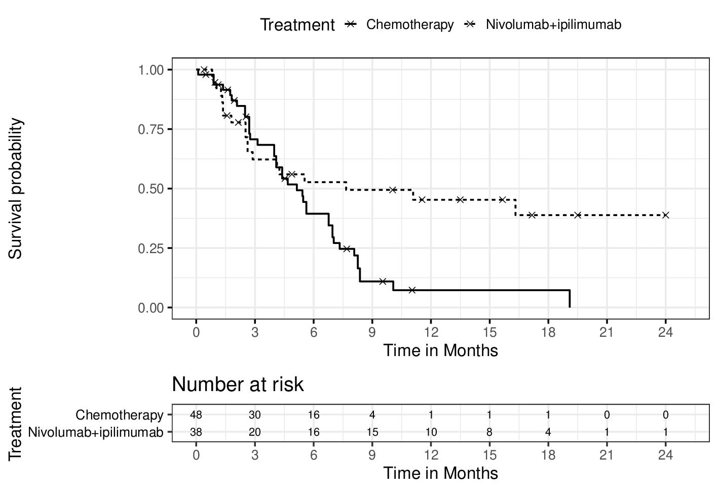
To illustrate the presented permutation-based methods, we re-consider the data analysis of Hellmann et al. 2018, who compared a combination treatment of nivolumab plus ipilimumab with chemotherapy among patients with non-small-cell lung cancer. Their study focused on patients with a high tumor mutational burden, i.e. at least ten mutations per megabase. And the study endpoint was progression-free survival. Since the present methods are designed for small sample sizes, we conduct a relevant subgroup analysis, which was also done by Hellmann et al. 2018. In detail, we restrict to the patients having PD-L1 (tumor programmed death ligand 1) expression of at least . On the basis of the published Kaplan–Meier curves in Hellmann et al. 2018 and some additional information therein, e.g. the risk table, we reconstructed the individual patient data following the procedure of Guyot et al. 2012. The respective Kaplan–Meier curves of the two treatment groups are displayed in Figure 4. Therein, we can observe a delayed treatment effect of nivolumab plus ipilimumab. Thus, the assumption of proportional hazards is questionable and can even by formally rejected by the well established test of Grambsch and Therneau 1994 or the recent permutation-based proposal of Ditzhaus and Janssen 2020 (with 10,000 permutations). Both tests lead to a -value less than . That is why the original analysis of Hellmann et al. 2018 using the hazard ratio (HR: and CI ) need to be considered carefully. The RMSTs offer the possibility to interpret the treatment effect easily beyond the Cox model. The -values of the asymptotic, studentized and unstudentized permutation tests (both based on 5,000 permutations), for inferring are presented in Table 2. The confidence intervals for the difference as well as for the ratio are shown in Table 3. In both tables, the different end points were considered. In practice, the end point needs to be chosen jointly with the physician regarding clinical relevance.
| months | months | months | |||||||
|---|---|---|---|---|---|---|---|---|---|
| Asym | un P | st P | Asym | un P | st P | Asym | un P | st P | |
| -values | 0.045 | 0.045 | 0.067 | 0.01 | 0.011 | 0.02 | 0.004 | 0.005 | 0.011 |
| months | months | months | ||||
| Asym | st P | Asym | st P | Asym | st P | |
| -1.85 | -2.99 | -4.02 | ||||
| -CI | [] | |||||
| 0.75 | 0.65 | 0.59 | ||||
| -CI | [0.57,0.98] | [0.56,1.01] | [0.48,0.88] | [0.47,0.91] | [0.43, 0.82] | [0.41,0.85] |
For and , the results confirm the findings of Hellmann et al. 2018 that the combination nivolumab plus ipilimumab improves the progression-free time compared to the chemotherapy. The point estimates and confidence intervals in Table 3 help to quantify the improvement and can be interpreted easily. For example, the combination treatment leads in average to a longer progression-free time of months ( confidence based on 5,000 permutations) compared to the chemotherapy over the first 1.5 years.
In general, it is observed that the asymptotic approach leads to smaller -values and narrower confidence intervals than its permutation counterpart. Moreover, the unstudentized permutation test lead to comparable -values than the asymptotic approach. As pointed out in Section 3, the results of the asymptotic and unstudentized permutation test need to be considered carefully, especially for small and unbalanced sample sizes as having here. Thus, we would rather trust the results of the studentized permutation test than those of the other two, especially for months, where the decisions are diverse.
5 Discussion and remarks
In the last years, the RMST became an important part of the statistical toolbox for survival data. Various researchers (Stensrud and Hernán 2020; Trinquart et al. 2016; A’Hern) advise to use it, at least, as a complementary summary statistic, especially when the assumption of proportional hazards is in doubt. As raised by Horiguchi and Uno 2020a, the type-I error rate of related asymptotic methods is inflated for small sample sizes. The permutation procedure of Horiguchi and Uno 2020a as well as their detailed discussion of how to deal with inestimable Kaplan–Meier curves of the permutated data was an important step to solve that problem. However, their test’s application is limited to exchangeable data settings and, in particular, to equal survival and censoring distributions, respectively.
In this paper, we explained how studentization can tackle these limitations. For the present survival two-sample comparison, it allows us to apply permutation tests even in non-exchangeable data situation, i.e. for different survival and/or censoring distributions, as well as to formulate corresponding confidence intervals for the quantity and of interest. Moreover, the control of the type-I error, which was the initial motivation for permutation tests, is not affected by the studentization strategy. Compared to their asymptotic counterparts, studentized permutation tests usually show a satisfactory type-I error control even for small sample sizes, as seen in Section 3.
The theoretical justification of studentized permutation tests and respective confidence intervals is complemented by an extensive simulation study. The corresponding results support the usage of the developed methods for small sample sizes.
Our framework can be extended in various directions, e.g. to competing risks (Zhao et al. 2018; Lyu et al. 2020). More general study designs may be part of future research. For that purpose, we can follow Dobler and Pauly 2020 and Ditzhaus et al. 2020a, who recently discussed permutation-based inference for the concordance measure and median survival times, respectively, in the general context of factorial designs. Sample size determination can also be developed, in parallel to the asymptotic test based results (Ye and Yu 2018).
Acknowledgement
Marc Ditzhaus was funded by the Deutsche Forschungsgemeinschaft (grant no. PA-2409 5-1). Moreover, the authors gratefully acknowledge the computing time provided on the Linux HPC cluster at TU Dortmund (LiDO3), partially funded in the course of the Large-Scale Equipment Initiative by the Deutsche Forschungsgemeinschaft as project 271512359.
References
- (1) R.P. A’Hern. Restricted mean survival time: an obligatory end point for time-to-event analysis in cancer trials? Journal of Clinical Oncology, 34(28):3474–3476.
- Alexander et al. (2018) B.M. Alexander, J.D. Schoenfeld, and L. Trippa. Hazards of hazard ratios-deviations from model assumptions in immunotherapy. The New England Journal of Medicine, 378(12):1158–1159, 2018.
- Andersen et al. (1993) P.K. Andersen, Ø. Borgan, R.D. Gill, and N. Keiding. Statistical Models Based on Counting Processes. Springer, New York, 1993.
- Berrett et al. (2020) T.B Berrett, Y. Wang, R. F. Barber, and R.J. Samworth. The conditional permutation test for independence while controlling for confounders. Journal of the Royal Statistical Society: Series B (Statistical Methodology), 82(1):175–197, 2020.
- Brookmeyer and Crowley (1982) R. Brookmeyer and J. Crowley. A confidence interval for the median survival time. Biometrics, 38:29–41, 1982.
- Chen and Zhang (2016) Z. Chen and G. Zhang. Comparing survival curves based on medians. BMC Medical Research Methodology, 16(1):1–7, 2016.
- Chung and Romano (2013) E.Y. Chung and J.P. Romano. Exact and asymptotically robust permutation tests. The Annals of Statistics, 41:484–507, 2013.
- Ditzhaus and Friedrich (2020) M. Ditzhaus and S. Friedrich. More powerful logrank permutation tests for two-sample survival data. Journal of Statistical Computation and Simulation, 90(12):2209–2227, 2020.
- Ditzhaus and Janssen (2020) M. Ditzhaus and A. Janssen. Bootstrap and permutation rank tests for proportional hazards under right censoring. Lifetime Data Analysis, 26(3):493–517, 2020.
- Ditzhaus et al. (2020a) M. Ditzhaus, D. Dobler, and M. Pauly. Inferring median survival differences in general factorial designs via permutation tests. Statistical Methods in Medical Research, page 0962280220980784, 2020a.
- Ditzhaus et al. (2020b) M. Ditzhaus, A. Janssen, and M. Pauly. Permutation inference in factorial survival designs with the CASANOVA. arXiv preprint arXiv:2004.10818, 2020b.
- Ditzhaus et al. (2021) M. Ditzhaus, R. Fried, and M. Pauly. QANOVA: Quantile-based permutation methods for general factorial designs. TEST (to appear), 2021.
- Dobler and Pauly (2018) D Dobler and M Pauly. Bootstrap-and permutation-based inference for the Mann–Whitney effect for right-censored and tied data. TEST, 27(3):639–658, 2018.
- Dobler and Pauly (2020) D. Dobler and M. Pauly. Factorial analyses of treatment effects under independent right-censoring. Statistical Methods in Medical Research, 29(2):325–343, 2020.
- Grambsch and Therneau (1994) P.M. Grambsch and T.M. Therneau. Proportional hazards tests and diagnostics based on weighted residuals. Biometrika, 81(3):515–526, 1994.
- Guyot et al. (2012) P. Guyot, A.E. Ades, M. Ouwens, and N.J. Welton. Enhanced secondary analysis of survival data: reconstructing the data from published Kaplan-Meier survival curves. BMC Medical Research Methodology, 12(1):1–13, 2012.
- Hellmann et al. (2018) M.D. Hellmann, T.-E. Ciuleanu, A. Pluzanski, J. S. Lee, G.A. Otterson, C. Audigier-Valette, E. Minenza, H. Linardou, S. Burgers, P. Salman, et al. Nivolumab plus ipilimumab in lung cancer with a high tumor mutational burden. New England Journal of Medicine, 378(22):2093–2104, 2018.
- Hemerik and Goeman (2018) J. Hemerik and J. Goeman. Exact testing with random permutations. TEST, 27(4):811–825, 2018.
- Horiguchi and Uno (2020a) M. Horiguchi and H. Uno. On permutation tests for comparing restricted mean survival time with small sample from randomized trials. Statistics in Medicine, 39(20):2655–2670, 2020a.
- Horiguchi and Uno (2020b) M. Horiguchi and H. Uno. survRM2perm: Permutation Test for Comparing Restricted Mean Survival Time, 2020b. URL https://CRAN.R-project.org/package=survRM2perm. R package version 0.1.0.
- Janssen (1997) A. Janssen. Studentized permutation tests for non-iid hypotheses and the generalized Behrens-Fisher problem. Statistics & Probability Letters, 36:9–21, 1997.
- Janssen and Pauls (2003) A. Janssen and T. Pauls. How do bootstrap and permutation tests work? Annals of Statistics, 31(3):768–806, 2003.
- Kim et al. (2017) D.H. Kim, H. Uno, and L.-J. Wei. Restricted mean survival time as a measure to interpret clinical trial results. JAMA Cardiology, 2(11):1179–1180, 2017.
- Lehmann and Romano (2006) E.L. Lehmann and J.P. Romano. Testing statistical hypotheses. Springer, New York, 2006.
- Lyu et al. (2020) J. Lyu, Y. Hou, and Z. Chen. The use of restricted mean time lost under competing risks data. BMC Medical Research Methodology, 20(1):1–11, 2020.
- Mick and Chen (2015) T. Mick and T.-T. Chen. Statistical challenges in the design of late-stage cancer immunotherapy studies. Cancer Immunology Research, 3(12):1292–1298, 2015.
- Neuhaus (1993) G. Neuhaus. Conditional rank tests for the two-sample problem under random censorship. The Annals of Statistics, 21:1760–1779, 1993.
- Pauly and Smaga (2020) M. Pauly and Ł. Smaga. Asymptotic permutation tests for coefficients of variation and standardised means in general one-way anova models. Statistical Methods in Medical Research, 29(9):2733–2748, 2020.
- Pauly et al. (2015) M. Pauly, E. Brunner, and F. Konietschke. Asymptotic permutation tests in general factorial designs. Journal of the Royal Statistical Society: Series B, 77:461–473, 2015.
- R Core Team (2021) R Core Team. R: A language and environment for statistical computing. R Foundation for Statistical Computing, Vienna, Austria, 2021. URL http://www.R-project.org.
- Royston and Parmar (2011) P. Royston and M.K.B. Parmar. The use of restricted mean survival time to estimate the treatment effect in randomized clinical trials when the proportional hazards assumption is in doubt. Statistics in Medicine, 30(19):2409–2421, 2011.
- Royston and Parmar (2013) P. Royston and M.K.B. Parmar. Restricted mean survival time: an alternative to the hazard ratio for the design and analysis of randomized trials with a time-to-event outcome. BMC Medical Research Methodology, 13(1):1–15, 2013.
- Scott et al. (2017) B.L. Scott, M.C. Pasquini, B.R. Logan, J. Wu, S.M. Devine, D.L. Porter, R.T. Maziarz, E.D. Warlick, H.F. Fernandez, E.P. Alyea, et al. Myeloablative versus reduced-intensity hematopoietic cell transplantation for acute myeloid leukemia and myelodysplastic syndromes. Journal of Clinical Oncology, 35(11):1154, 2017.
- Smaga (2017) Ł. Smaga. Diagonal and unscaled Wald-type tests in general factorial designs. Electronic Journal of Statistics, 11(1):2613–2646, 2017.
- Stensrud and Hernán (2020) M.J. Stensrud and M.A. Hernán. Why test for proportional hazards? JAMA, 323(14):1401–1402, 2020.
- Taori et al. (2009) G. Taori, K.M. Ho, C. George, R. Bellomo, S.A.R. Webb, G.K. Hart, and M.J. Bailey. Landmark survival as an end-point for trials in critically ill patients–comparison of alternative durations of follow-up: an exploratory analysis. Critical Care, 13(4):1–8, 2009.
- Tian et al. (2020) L. Tian, H. Jin, H. Uno, Y. Lu, B. Huang, K. M. Anderson, and L.J. Wei. On the empirical choice of the time window for restricted mean survival time. Biometrics, 2020.
- Trinquart et al. (2016) L. Trinquart, J. Jacot, S.C. Conner, and R. Porcher. Comparison of treatment effects measured by the hazard ratio and by the ratio of restricted mean survival times in oncology randomized controlled trials. Journal of Clinical Oncology, 34(15):1813–1819, 2016.
- Uno et al. (2014) H. Uno, B. Claggett, L. Tian, E. Inoue, P. Gallo, T. Miyata, D. Schrag, M. Takeuchi, Y. Uyama, L. Zhao, et al. Moving beyond the hazard ratio in quantifying the between-group difference in survival analysis. Journal of Clinical Oncology, 32(22):2380, 2014.
- van der Vaart and Wellner (1996) A.W. van der Vaart and J.A. Wellner. Weak convergence and empirical processes. Springer Series in Statistics. Springer-Verlag, New York, 1996. With applications to statistics.
- Ye and Yu (2018) T. Ye and M. Yu. A robust approach to sample size calculation in cancer immunotherapy trials with delayed treatment effect. Biometrics, 74(4):1292–1300, 2018.
- Zhao et al. (2016) L. Zhao, B. Claggett, L. Tian, H. Uno, M.A. Pfeffer, S.D. Solomon, L. Trippa, and L.J. Wei. On the restricted mean survival time curve in survival analysis. Biometrics, 72(1):215–221, 2016.
- Zhao et al. (2018) L. Zhao, L. Tian, B. Claggett, M. Pfeffer, D. H. Kim, S. Solomon, and L.-J. Wei. Estimating treatment effect with clinical interpretation from a comparative clinical trial with an end point subject to competing risks. JAMA Cardiology, 3(4):357–358, 2018.
- Zittoun et al. (1995) R.A. Zittoun, F. Mandelli, R. Willemze, T. De Witte, B. Labar, L. Resegotti, F. Leoni, E. Damasio, G. Visani, G. Papa, et al. Autologous or allogeneic bone marrow transplantation compared with intensive chemotherapy in acute myelogenous leukemia. New England Journal of Medicine, 332(4):217–223, 1995.
Appendix A Additional simulation results
First, we present the results for the power comparison, see Tables 5–7, and for the type-I error comparison in Table 4 under the remaining censoring setting C3, i.e. equally Weibull distributed censoring. The results were already briefly discussed in the main paper, including all relevant main conclusions. In addition to that, we present here the simulation results of the asymptotic and permutation-based confidence intervals for the ratio from Section 2.2. For the respective simulation study, we used the same set-up as in the simulation study for the difference-based methods from Section 3. In particular, each boxplot in Figure 5 summarizes the results for different settings. It is apparent that the performance of the asymptotic confidence interval is less extreme than the one for the differences. But for small sample sizes, here , it still leads to an undercoverage or liberal decisions. For the moderate sample sizes, the undercoverage almost vanishes and, for the large sample sizes, it completely vanishes with just a few exceptions. The permutation-based confidence intervals lead to more stable results, especially under with and, thus, it is still our recommendation for sample sizes .
| Cens. rates | Asym | st P | un P | Asym | st P | un P | Asym | st P | un P | ||
|---|---|---|---|---|---|---|---|---|---|---|---|
| S1 and S2: Exponential | |||||||||||
| (11, 11) | 1 | 6.1 | 4.6 | 4.7 | 6.4 | 5.0 | 5.0 | 5.9 | 4.7 | 4.7 | |
| 2 | 5.8 | 4.9 | 5.0 | 5.7 | 5.0 | 5.0 | 5.6 | 4.6 | 4.8 | ||
| 4 | 5.5 | 5.0 | 5.1 | 4.7 | 4.4 | 4.5 | 5.4 | 5.0 | 5.0 | ||
| S3: Exponential vs. piece-wise Exponential (crossing curves) | |||||||||||
| (11, 27) | 1 | 7.7 | 5.9 | 7.2 | 6.3 | 4.9 | 5.0 | 6.4 | 4.7 | 3.9 | |
| 2 | 6.1 | 5.5 | 6.7 | 5.3 | 4.8 | 4.9 | 5.9 | 5.1 | 3.8 | ||
| 4 | 5.7 | 5.3 | 6.6 | 5.8 | 5.4 | 5.4 | 6.1 | 5.9 | 4.7 | ||
| S4: Lognormal | |||||||||||
| (21,21) | 1 | 6.3 | 5.1 | 4.8 | 5.9 | 4.6 | 4.8 | 7.5 | 5.5 | 5.6 | |
| 2 | 5.8 | 4.9 | 5.2 | 5.4 | 4.7 | 4.8 | 5.3 | 4.7 | 4.7 | ||
| 4 | 5.2 | 4.7 | 4.8 | 5.4 | 5.1 | 5.1 | 5.3 | 5.0 | 4.9 | ||
| S5: Weibull (different shape) | |||||||||||
| (13,40) | 1 | 7.5 | 5.7 | 7.7 | 7.2 | 5.7 | 5.6 | 6.2 | 4.6 | 3.2 | |
| 2 | 5.9 | 4.9 | 7.1 | 5.6 | 5.2 | 4.9 | 5.8 | 5.0 | 3.5 | ||
| 4 | 5.3 | 5.0 | 6.9 | 5.1 | 4.7 | 4.9 | 5.3 | 5.0 | 3.3 | ||
| S6: Weibull (different scale) | |||||||||||
| (13,26) | 1 | 6.6 | 4.9 | 6.0 | 6.1 | 4.8 | 4.8 | 6.4 | 4.8 | 3.7 | |
| 2 | 6.6 | 5.9 | 7.0 | 5.3 | 4.6 | 4.6 | 5.5 | 4.6 | 3.5 | ||
| 4 | 5.3 | 5.0 | 6.4 | 5.3 | 5.0 | 5.1 | 5.0 | 4.9 | 3.6 | ||
| S7: Weibull vs. piece-wise Exponential | |||||||||||
| (11, 43) | 1 | 6.5 | 4.7 | 6.4 | 7.1 | 5.6 | 5.6 | 6.2 | 4.9 | 3.5 | |
| 2 | 6.7 | 6.1 | 7.5 | 5.9 | 5.2 | 5.2 | 5.3 | 4.5 | 3.0 | ||
| 4 | 4.9 | 4.6 | 6.3 | 5.2 | 5.0 | 5.1 | 5.2 | 4.8 | 3.7 | ||
| Cens. Distr | Cens. rates | Asym | st P | un P | Asym | st P | un P | Asym | st P | un P | ||
|---|---|---|---|---|---|---|---|---|---|---|---|---|
| S1: Exponential (proportional hazards) | ||||||||||||
| Weib (uneq) | (7,30) | 1 | 15.3 | 12.2 | 15.1 | 15.3 | 12.5 | 13.6 | 16.1 | 12.6 | 12.2 | |
| 2 | 23.3 | 21.4 | 24.6 | 23.8 | 21.8 | 22.9 | 23.8 | 21.6 | 20.6 | |||
| 4 | 38.9 | 37.4 | 41.7 | 41.2 | 40.0 | 41.4 | 41.1 | 39.4 | 38.1 | |||
| (7,34) | 1 | 40.6 | 35.2 | 40.2 | 42.3 | 37.7 | 39.0 | 42.8 | 37.0 | 36.2 | ||
| 2 | 64.0 | 61.4 | 65.9 | 69.2 | 67.1 | 68.3 | 67.3 | 65.0 | 63.9 | |||
| 4 | 90.1 | 89.4 | 91.4 | 92.5 | 92.2 | 92.5 | 92.4 | 91.9 | 91.2 | |||
| Unif (eq) | (20,27) | 1 | 16.0 | 12.3 | 13.7 | 16.3 | 13.8 | 13.8 | 18.1 | 14.2 | 13.3 | |
| 2 | 24.1 | 22.0 | 23.3 | 25.7 | 23.6 | 23.5 | 25.3 | 23.1 | 22.3 | |||
| 4 | 41.3 | 40.3 | 41.4 | 41.5 | 40.4 | 40.4 | 42.4 | 41.4 | 40.0 | |||
| (20,37) | 1 | 41.7 | 35.4 | 38.0 | 43.6 | 38.5 | 38.7 | 42.2 | 36.9 | 36.1 | ||
| 2 | 65.8 | 63.5 | 64.9 | 69.9 | 68.0 | 67.9 | 67.8 | 65.2 | 64.7 | |||
| 4 | 91.2 | 90.6 | 91.1 | 92.8 | 92.4 | 92.3 | 91.6 | 91.2 | 91.1 | |||
| Weib (eq) | (11,19) | 1 | 16.8 | 13.5 | 15.0 | 16.1 | 13.7 | 13.7 | 17.5 | 14.5 | 13.7 | |
| 2 | 26.0 | 24.1 | 25.3 | 26.6 | 24.8 | 24.9 | 25.3 | 23.3 | 22.8 | |||
| 4 | 41.6 | 40.8 | 41.7 | 46.1 | 44.8 | 44.9 | 44.6 | 43.3 | 42.4 | |||
| (11,29) | 1 | 44.9 | 40.3 | 42.1 | 47.0 | 42.0 | 42.1 | 44.9 | 40.1 | 39.2 | ||
| 2 | 71.6 | 69.4 | 70.9 | 72.4 | 70.6 | 70.3 | 72.2 | 69.6 | 69.0 | |||
| 4 | 93.4 | 93.0 | 93.5 | 95.1 | 95.0 | 95.0 | 94.2 | 93.8 | 93.4 | |||
| S2: Exponential (late departures) | ||||||||||||
| Weib (uneq) | (7,30) | 1 | 13.8 | 10.9 | 14.2 | 14.8 | 12.1 | 13.3 | 16.2 | 12.8 | 11.5 | |
| 2 | 20.9 | 19.1 | 23.8 | 21.7 | 20.0 | 21.4 | 23.2 | 21.2 | 19.5 | |||
| 4 | 36.1 | 34.7 | 40.2 | 39.6 | 38.5 | 40.3 | 38.9 | 37.9 | 35.5 | |||
| (7,39) | 1 | 34.8 | 30.2 | 36.6 | 37.8 | 32.8 | 34.7 | 38.1 | 32.7 | 30.1 | ||
| 2 | 56.1 | 53.2 | 60.3 | 61.7 | 59.4 | 61.2 | 62.7 | 59.6 | 57.2 | |||
| 4 | 84.8 | 84.0 | 87.9 | 88.3 | 87.7 | 88.6 | 87.7 | 87.1 | 85.6 | |||
| Unif (eq) | (20,31) | 1 | 14.8 | 11.2 | 13.1 | 15.1 | 12.3 | 12.3 | 15.8 | 12.9 | 11.1 | |
| 2 | 22.0 | 20.3 | 22.2 | 23.8 | 21.8 | 22.2 | 24.2 | 22.0 | 19.9 | |||
| 4 | 36.5 | 35.3 | 37.3 | 39.4 | 38.2 | 38.1 | 37.8 | 36.6 | 34.1 | |||
| (20,49) | 1 | 36.8 | 31.3 | 34.5 | 38.3 | 33.9 | 33.4 | 38.6 | 33.5 | 30.7 | ||
| 2 | 59.5 | 56.9 | 59.8 | 62.5 | 60.1 | 59.8 | 61.8 | 59.4 | 56.2 | |||
| 4 | 85.7 | 84.8 | 86.4 | 88.6 | 87.9 | 88.0 | 89.4 | 88.6 | 86.6 | |||
| Weib (eq) | (11,24) | 1 | 15.4 | 12.5 | 14.6 | 16.2 | 13.4 | 13.3 | 15.7 | 12.8 | 11.5 | |
| 2 | 22.6 | 20.6 | 23.0 | 24.3 | 22.3 | 22.6 | 24.8 | 23.0 | 20.6 | |||
| 4 | 38.8 | 37.5 | 40.0 | 42.1 | 41.1 | 41.0 | 42.2 | 40.9 | 38.7 | |||
| (11,46) | 1 | 38.4 | 33.8 | 37.2 | 41.0 | 36.8 | 36.8 | 40.8 | 36.4 | 33.5 | ||
| 2 | 62.4 | 60.1 | 63.3 | 65.8 | 63.9 | 63.8 | 66.4 | 64.1 | 61.1 | |||
| 4 | 88.3 | 87.8 | 89.4 | 90.7 | 90.0 | 90.1 | 91.2 | 90.7 | 89.0 | |||
| S3: Exponential vs. piece-wise Exponential (crossing curves) | ||||||||||||
| Weib (uneq) | (7,32) | 1 | 14.3 | 11.5 | 15.1 | 14.3 | 11.8 | 12.6 | 15.1 | 12.0 | 10.0 | |
| 2 | 18.7 | 16.9 | 21.9 | 21.2 | 19.4 | 21.1 | 21.6 | 19.5 | 17.3 | |||
| 4 | 31.0 | 29.8 | 37.1 | 32.6 | 31.7 | 33.2 | 35.3 | 34.2 | 30.9 | |||
| (7,36) | 1 | 36.3 | 31.4 | 37.3 | 38.6 | 33.6 | 35.1 | 38.9 | 33.4 | 30.9 | ||
| 2 | 57.7 | 54.9 | 61.9 | 61.1 | 58.6 | 60.0 | 61.7 | 59.2 | 55.8 | |||
| 4 | 85.1 | 84.7 | 87.5 | 87.5 | 86.8 | 87.5 | 88.6 | 88.0 | 86.3 | |||
| Unif (eq) | (20,38) | 1 | 13.7 | 10.8 | 12.5 | 14.3 | 11.4 | 11.2 | 15.8 | 13.1 | 10.8 | |
| 2 | 20.7 | 18.8 | 21.5 | 20.5 | 18.6 | 18.4 | 21.6 | 19.7 | 16.4 | |||
| 4 | 34.1 | 32.8 | 36.5 | 34.6 | 33.6 | 33.2 | 36.2 | 34.9 | 30.9 | |||
| (20,46) | 1 | 36.8 | 31.4 | 34.9 | 38.6 | 33.9 | 33.7 | 38.2 | 33.4 | 30.6 | ||
| 2 | 59.8 | 56.8 | 60.1 | 62.2 | 59.7 | 59.6 | 62.5 | 59.7 | 56.7 | |||
| 4 | 86.5 | 85.7 | 87.5 | 89.3 | 88.8 | 88.5 | 88.5 | 87.7 | 86.0 | |||
| Weib (eq) | (11,35) | 1 | 14.3 | 11.9 | 14.0 | 14.9 | 12.6 | 12.6 | 14.7 | 11.9 | 9.8 | |
| 2 | 20.9 | 19.1 | 22.0 | 22.3 | 20.8 | 20.9 | 23.4 | 21.8 | 18.3 | |||
| 4 | 33.5 | 32.7 | 36.7 | 38.5 | 37.7 | 37.7 | 37.3 | 36.2 | 32.4 | |||
| (11,42) | 1 | 38.0 | 33.0 | 36.7 | 39.5 | 35.3 | 35.4 | 41.5 | 36.5 | 33.8 | ||
| 2 | 61.6 | 58.9 | 62.6 | 64.2 | 62.0 | 62.3 | 65.5 | 63.0 | 59.6 | |||
| 4 | 88.5 | 87.9 | 89.9 | 91.3 | 90.9 | 90.8 | 90.4 | 89.9 | 88.2 | |||
| Cens. Distr | Cens. rates | Asym | st P | un P | Asym | st P | un P | Asym | st P | un P | ||
|---|---|---|---|---|---|---|---|---|---|---|---|---|
| S4: Lognormal (scale alternatives) | ||||||||||||
| Weib (uneq) | (14,39) | 1 | 30.2 | 25.5 | 24.2 | 28.4 | 24.1 | 23.1 | 27.3 | 22.5 | 22.5 | |
| 2 | 45.7 | 42.9 | 43.5 | 45.3 | 42.8 | 42.2 | 45.1 | 41.5 | 40.9 | |||
| 4 | 70.6 | 69.5 | 70.6 | 72.0 | 71.1 | 71.3 | 71.8 | 70.6 | 69.8 | |||
| (12,44) | 1 | 83.0 | 79.1 | 76.7 | 84.5 | 80.8 | 79.2 | 82.5 | 76.9 | 77.9 | ||
| 2 | 98.2 | 97.7 | 97.6 | 98.5 | 98.2 | 98.0 | 98.1 | 97.6 | 97.6 | |||
| 4 | 100.0 | 100.0 | 100.0 | 100.0 | 100.0 | 100.0 | 100.0 | 100.0 | 100.0 | |||
| Unif (eq) | (33,42) | 1 | 27.3 | 22.1 | 20.6 | 26.5 | 22.2 | 22.1 | 25.5 | 20.4 | 22.9 | |
| 2 | 42.7 | 39.9 | 38.1 | 43.2 | 40.6 | 40.3 | 42.5 | 38.9 | 41.2 | |||
| 4 | 69.9 | 68.7 | 67.6 | 71.6 | 70.5 | 70.3 | 68.6 | 67.3 | 68.8 | |||
| (33,56) | 1 | 81.7 | 77.2 | 74.2 | 81.4 | 77.3 | 77.5 | 76.6 | 70.2 | 76.7 | ||
| 2 | 97.7 | 97.1 | 96.5 | 97.8 | 97.4 | 97.5 | 96.4 | 95.5 | 96.8 | |||
| 4 | 100.0 | 100.0 | 100.0 | 100.0 | 100.0 | 100.0 | 100.0 | 100.0 | 100.0 | |||
| Weib (eq) | (21,32) | 1 | 32.8 | 28.5 | 26.2 | 30.8 | 27.2 | 27.2 | 29.3 | 24.5 | 27.4 | |
| 2 | 50.4 | 47.6 | 45.5 | 50.4 | 48.0 | 48.3 | 45.8 | 43.5 | 45.8 | |||
| 4 | 78.2 | 77.0 | 75.9 | 78.2 | 77.3 | 77.5 | 75.5 | 74.8 | 75.9 | |||
| (21,52) | 1 | 87.8 | 84.6 | 82.2 | 87.5 | 84.4 | 84.2 | 84.5 | 80.7 | 85.1 | ||
| 2 | 99.2 | 99.1 | 98.9 | 99.3 | 99.2 | 99.1 | 98.8 | 98.5 | 98.9 | |||
| 4 | 100.0 | 100.0 | 100.0 | 100.0 | 100.0 | 100.0 | 100.0 | 100.0 | 100.0 | |||
| S5: Weibull (different shape) | ||||||||||||
| Weib (uneq) | (8,40) | 1 | 25.8 | 22.4 | 25.7 | 25.0 | 22.0 | 22.7 | 24.5 | 20.3 | 19.4 | |
| 2 | 35.7 | 33.4 | 39.7 | 38.5 | 36.3 | 38.1 | 37.1 | 35.0 | 32.8 | |||
| 4 | 55.7 | 54.7 | 62.0 | 60.1 | 59.1 | 61.8 | 62.5 | 60.8 | 57.9 | |||
| (8,42) | 1 | 75.4 | 71.5 | 73.3 | 77.2 | 73.2 | 73.1 | 77.8 | 72.7 | 72.3 | ||
| 2 | 94.9 | 94.1 | 95.4 | 96.0 | 95.6 | 95.8 | 96.1 | 95.3 | 95.2 | |||
| 4 | 99.9 | 99.8 | 99.9 | 99.9 | 99.9 | 99.9 | 100.0 | 99.9 | 99.9 | |||
| Unif (eq) | (29,48) | 1 | 25.0 | 20.5 | 21.6 | 25.2 | 20.6 | 20.6 | 23.9 | 19.4 | 18.1 | |
| 2 | 35.8 | 33.3 | 35.2 | 37.9 | 35.3 | 34.8 | 38.4 | 35.5 | 33.6 | |||
| 4 | 59.0 | 57.7 | 60.4 | 60.9 | 59.8 | 59.2 | 61.2 | 59.9 | 56.3 | |||
| (29,50) | 1 | 75.5 | 70.6 | 70.0 | 77.2 | 72.9 | 72.8 | 74.5 | 67.7 | 70.3 | ||
| 2 | 94.3 | 93.5 | 93.7 | 96.3 | 95.6 | 95.8 | 95.6 | 94.6 | 94.7 | |||
| 4 | 99.9 | 99.9 | 99.9 | 99.9 | 99.9 | 99.9 | 100.0 | 100.0 | 100.0 | |||
| Weib (eq) | (13,42) | 1 | 26.4 | 22.9 | 23.9 | 27.5 | 24.2 | 24.0 | 26.1 | 22.4 | 21.3 | |
| 2 | 40.2 | 37.9 | 40.8 | 40.3 | 38.2 | 38.1 | 43.0 | 40.9 | 37.9 | |||
| 4 | 63.0 | 61.6 | 65.0 | 68.3 | 67.4 | 67.4 | 67.9 | 66.9 | 63.4 | |||
| (13,44) | 1 | 81.0 | 77.3 | 77.4 | 81.6 | 78.4 | 78.3 | 82.2 | 78.5 | 79.3 | ||
| 2 | 97.5 | 96.9 | 97.2 | 98.0 | 97.6 | 97.7 | 97.9 | 97.7 | 97.6 | |||
| 4 | 100.0 | 100.0 | 100.0 | 100.0 | 100.0 | 100.0 | 100.0 | 100.0 | 100.0 | |||
| Cens. Distr | Cens. rates | Asym | st P | un P | Asym | st P | un P | Asym | st P | un P | ||
|---|---|---|---|---|---|---|---|---|---|---|---|---|
| S6: Weibull (different scale) | ||||||||||||
| Weib (uneq) | (8,40) | 1 | 25.3 | 21.7 | 25.5 | 24.8 | 21.2 | 22.0 | 23.5 | 19.2 | 18.2 | |
| 2 | 35.5 | 33.2 | 39.7 | 38.9 | 36.8 | 38.7 | 38.1 | 35.4 | 33.3 | |||
| 4 | 57.3 | 55.9 | 63.7 | 61.2 | 60.0 | 62.1 | 62.7 | 60.8 | 57.8 | |||
| (8,48) | 1 | 70.5 | 66.1 | 70.0 | 72.3 | 68.5 | 69.0 | 73.5 | 68.2 | 66.7 | ||
| 2 | 90.4 | 89.2 | 92.0 | 92.3 | 91.5 | 92.0 | 93.7 | 92.6 | 91.6 | |||
| 4 | 99.7 | 99.5 | 99.8 | 99.8 | 99.7 | 99.8 | 99.9 | 99.9 | 99.9 | |||
| Unif (eq) | (29,48) | 1 | 24.5 | 20.3 | 21.4 | 24.5 | 20.5 | 20.2 | 23.8 | 19.0 | 18.2 | |
| 2 | 36.1 | 33.7 | 35.4 | 37.6 | 35.2 | 34.9 | 37.1 | 34.3 | 31.8 | |||
| 4 | 57.9 | 56.5 | 59.4 | 61.2 | 60.0 | 59.7 | 61.4 | 60.1 | 56.7 | |||
| (29,67) | 1 | 69.6 | 64.5 | 65.2 | 73.0 | 68.3 | 67.8 | 69.4 | 63.6 | 64.1 | ||
| 2 | 91.6 | 90.7 | 91.0 | 92.8 | 91.9 | 91.8 | 92.5 | 91.5 | 90.8 | |||
| 4 | 99.6 | 99.5 | 99.7 | 99.9 | 99.9 | 99.8 | 99.8 | 99.8 | 99.8 | |||
| Weib (eq) | (13,42) | 1 | 26.5 | 22.9 | 24.3 | 25.8 | 22.3 | 22.2 | 26.5 | 22.5 | 21.4 | |
| 2 | 40.4 | 38.0 | 40.5 | 42.4 | 40.6 | 40.2 | 42.1 | 39.4 | 36.8 | |||
| 4 | 63.7 | 62.6 | 65.7 | 67.9 | 66.8 | 66.5 | 68.2 | 67.1 | 63.4 | |||
| (13,65) | 1 | 74.9 | 71.2 | 72.9 | 77.7 | 74.1 | 73.6 | 75.8 | 71.7 | 71.7 | ||
| 2 | 94.3 | 93.4 | 94.5 | 96.0 | 95.6 | 95.6 | 95.3 | 94.7 | 94.1 | |||
| 4 | 99.8 | 99.8 | 99.8 | 100.0 | 100.0 | 100.0 | 99.9 | 99.9 | 99.8 | |||
| S7: Weibull vs. piece-wise Exponential | ||||||||||||
| Weib (uneq) | (7,46) | 1 | 16.9 | 14.3 | 18.0 | 17.4 | 14.5 | 15.6 | 17.5 | 14.6 | 12.4 | |
| 2 | 24.2 | 22.3 | 28.9 | 26.3 | 24.6 | 26.0 | 24.9 | 22.5 | 19.1 | |||
| 4 | 37.0 | 36.1 | 44.4 | 42.3 | 41.0 | 43.5 | 43.4 | 42.0 | 38.0 | |||
| (7,52) | 1 | 46.1 | 41.7 | 47.3 | 49.8 | 45.4 | 45.9 | 49.3 | 43.4 | 39.8 | ||
| 2 | 70.0 | 67.4 | 74.3 | 74.0 | 72.0 | 72.9 | 75.1 | 72.9 | 68.6 | |||
| 4 | 92.2 | 91.9 | 94.5 | 95.4 | 95.0 | 95.5 | 95.9 | 95.6 | 94.4 | |||
| Unif (eq) | (25,59) | 1 | 17.4 | 14.3 | 16.1 | 17.2 | 14.4 | 13.9 | 17.5 | 14.0 | 11.8 | |
| 2 | 25.1 | 23.2 | 25.9 | 26.0 | 24.0 | 23.4 | 25.8 | 23.5 | 19.5 | |||
| 4 | 38.2 | 37.1 | 40.9 | 40.5 | 39.6 | 38.7 | 44.3 | 43.0 | 37.5 | |||
| (25,69) | 1 | 48.6 | 43.6 | 46.0 | 49.1 | 44.7 | 43.5 | 48.6 | 42.9 | 40.3 | ||
| 2 | 71.9 | 69.4 | 72.6 | 73.3 | 71.2 | 70.1 | 76.0 | 73.8 | 69.6 | |||
| 4 | 93.2 | 92.9 | 94.1 | 95.5 | 95.1 | 95.0 | 96.0 | 95.5 | 94.2 | |||
| Weib (eq) | (11,56) | 1 | 18.0 | 14.9 | 17.8 | 18.9 | 15.9 | 15.8 | 17.8 | 14.5 | 12.3 | |
| 2 | 26.3 | 24.7 | 28.5 | 27.5 | 25.1 | 25.1 | 28.0 | 25.8 | 21.9 | |||
| 4 | 41.5 | 40.3 | 45.7 | 44.1 | 43.2 | 42.9 | 46.3 | 45.1 | 39.5 | |||
| (11,67) | 1 | 50.7 | 45.9 | 50.1 | 51.7 | 47.5 | 47.3 | 53.4 | 48.1 | 44.7 | ||
| 2 | 71.9 | 70.1 | 74.1 | 78.3 | 76.7 | 76.6 | 79.1 | 76.8 | 73.2 | |||
| 4 | 95.0 | 94.8 | 95.8 | 96.1 | 95.8 | 95.9 | 96.7 | 96.5 | 95.6 | |||

Appendix B Counting process notation
For the proofs, we adopt the counting process notation of Andersen et al. 1993. Let be the number of observed events up until in group and denotes the number of individuals under risk just before in group . Moreover, let and be the respective versions for the pooled sample. It is easy to check that
| (4) |
Given the counting process notation, we can write the Kaplan–Meier and Nelson–Aalen estimators as follows
where is the increment of in and are the distinctive time points within the observed times of group . Moreover, we introduce their pooled counterparts:
where are the distinctive time points within the pooled observation times .
Appendix C Proof of (1) and (3)
The convergence in (1) and (3) directly follow from the continuous mapping theorem, the -method and the following Proposition.
Proposition 1.
As , with variance
| (5) |
Proof of Proposition 1.
Let be the Skorohod space consisting of all càdlàg functions on . By Example 3.9.31 of van der Vaart and Wellner 1996
| (6) |
for a centered Gaussian process with covariance structure
Thus, we can deduce from (6) and the continuous mapping theorem
By Fubini’s Theorem (van der Vaart and Wellner 1996, Sec. 3.9.2), is indeed centered normally distributed with variance given by
∎
Appendix D Proof of the variance estimator’s consistency
Define and by . By the Glivenko–Cantelli Theorem
| (7) |
almost surely. It is well known that this combined with the continuous mapping theorem implies the uniform consistency of the Kaplan–Meier and Nelson–Aalen estimators:
| (8) |
almost surely. Obviously, it follows that
| (9) |
almost surely. In particular,
| (10) |
with probability one. Moreover, we can deduce from (4), (7) and (9) that we have almost surely as
| (11) |
Clearly, the consistency of follows. In the same way, we can deduce the consistency of which was defined after Equation (3).
Appendix E Proof of Theorems 1 and 2
We first introduce the limits of , and :
where and were already defined in the proof of Proposition 1. In fact, from the Glivenko-Cantelli Theorem (and the continuous mapping theorem for the convergence of ) we obtain immediately
| (12) |
with probability one as . In particular,
almost surely as .
For the first step of the proof, we follow the argumentation of the previous proof of (1). As explained by Dobler and Pauly 2018 (see Theorem 5 in their supplement), the following conditional convergence is a straightforward consequence of Theorems 3.7.1 and 3.7.2 in van der Vaart and Wellner 1996:
given the data in probability, where is a centered Gaussian process on with covariance structure given by
Consequently, we obtain from the continuous mapping theorem that given the data in probability
| (13) |
where is dimensional, centered normally distributed with covariance structure
Applying again the continuous mapping theorem yields that given the data in probability
| (14) |
This proves Theorem 1.
To verify Theorem 2, it remains to discuss the consistency of the variance estimator. Therefor, we fix the original observations . Note that , and does not change when permuting the data. Thus, we can treat them all as fixed functions. Moreover, we can assume without a loss of generality that (12) holds for them. Following (Neuhaus 1993, equation 6.1), we can deduce
Using similar arguments, the statement remains true for . Combining both, (12) and the continuous mapping theorem yields
In particular, we obtain
Combining all previous statements yields that as
Finally, the desired convergence of the variance estimator follows, i.e. as
Appendix F Proof of Corollary 2
It is sufficient to show that given the data in probability
| (15) |
The corresponding proof can again be separated into two steps: (1) verification of the asymptotic normality of and (2) showing the consistency of the variance estimator . It is easy to see that (1) follows immediately from (13) and the -method. Moreover, (2) can be proven in the same way as in the previous proof and, thus, it is omitted here.