$\mathbb{T}$-Operator Limits on Optical Communication:
Metaoptics, Computation, and Input–Output Transformations

Following the sketch provided in Ref. Molesky et al. 2020a (supporting details can be found in Refs. Tsang et al. 2004, Kirsch and Lechleiter 2009, Costabel et al. 2012, Krüger et al. 2012, Colton and Kress 2019), there are two superficial distinctions that distinguish a scattering theory view of electromagnetics from Maxwell’s equations. First, supposing a local, linear scattering potential, the fundamental wave relation from which all field properties are derived is

where the $s$ subscript denotes projection into the scattering object, $\mathbb{G}^{\text{0}}$ is the background Green’s function of the design domain $\Omega_{s}$, throughout taken to be the vacuum Green’s function (truncated to a problem-specific volume) scaled by $k_{o}^{2}=\left(2\pi/\lambda\right)^{2}$ (so that all spatial dimensions may be simply defined relative to the wavelength), $\mathbb{V}$ is the bulk (spatially local) scattering potential of the material forming the design, $\mathbb{I}$ is the identity operator, and $\mathbb{T}_{s}$ is the scattering operator, formally defined by Eq.(4) ¹¹ 1 All operators and fields are supposed to be frequency dependent, and every stated relation holds at any given frequency.²² 2 The potential of the scatterer is constructed via the explicit spatial projection operator $\mathbb{I}_{s}$, which is defined to be identity at spatial locations within the scatterer and zero at all other points in the domain $\Omega$, and the implicit spatial projection into the scattering object encoded in the definition the scattering operator, $\mathbb{T}_{s}$.. (Although more general descriptions are possible, it is implicitly assumed throughout this article that $\mathbb{V}=\mathbb{I}\chi$, where $\chi$ is electric susceptibility of some isotropic medium.) Second, one of either the electromagnetic field or polarization field is singled out as an initial ³³ 3 The specification of an initial field is essentially equivalent to the introduction of a source, or flux boundary condition, in Maxwell’s equations., and all other fields are generated via the scattering operator $\mathbb{T}_{s}$. This leads to a division of the theory into two classes: initial flux problems, where a far-field incident flux $\big|\textbf{E}^{i}\big>$ is assumed, generating a polarization current $\left|\textbf{J}^{g}\right>=-\left(ik_{o}/Z\right)\mathbb{T}_{s}\big|\textbf{E}^{i}\big>$ and scattered field $\big|\textbf{E}^{s}\big>=\left(iZ/k_{o}\right)\mathbb{G}^{\text{0}}\big|\textbf{J}^{g}\big>$, and initial source problems, where a polarization source $\big|\textbf{J}^{i}\big>$ is assumed, generating an electromagnetic field $\left|\textbf{E}^{g}\right>=\left(iZ/k_{o}\right)\mathbb{G}^{\text{0}}\mathbb{T}_{s}\mathbb{V}^{-1}\big|\textbf{J}^{i}\big>$ and total current $\big|\textbf{J}^{t}\big>=\mathbb{T}_{s}\mathbb{V}^{-1}\big|\textbf{J}^{i}\big>$.

Given that most quantities related to power transfer result from inner products between electromagnetic and polarization fields Tsang et al. 2004, many common design objectives within scattering theory, encompassing applications varying from enhancing the amount of radiation that can be extracted from a quantum emitter Liu et al. 2017, Koenderink 2017, Cox et al. 2018 to increasing absorption into a photovoltaic cell Mokkapati and Catchpole 2012, Sheng et al. 2012, Ganapati et al. 2013, are given by sesquilinear forms on the scattering operator $\mathbb{T}_{s}$. As the central example investigated in this article, continuing the discussion of Sec. I and covering all the specific applications treated in Sec. III, suppose that a collection of fluxes $\left\{\big|\textbf{E}^{i}_{k}\big>\right\}$, with $k$ ranging over some finite indexing set, is incident on a scattering design region $\Omega$. Assume that the goal of the (input–output) device is to create a set $\Big\{\big|\textbf{E}^{\diamond}_{k}\big>\Big\}$ of target fields within an observation region $\Omega_{o}$, marked by a domain subscript $o$ and spatial projection operator $\mathbb{I}_{o}$, i.e. a collection of register mappings $\big|\textbf{E}^{i}_{k}\big>\mapsto\big|\textbf{E}^{\diamond}_{k}\big>$. Taking the Euclidean norm as a metric of design performance,

the equivalent objective (in the sense (5) and (6) have the same minimum)

is effectively a sesquilinear form on $\mathbb{T}_{s}$.

and the objective of the design amounts to a minimization of

Here, $\operatorname{Sym}\left[\mathbb{O}\right]$ and $\operatorname{Asym}\left[\mathbb{O}\right]$ denote symmetric (Hermitian) and anti-symmetric (skew-hermitian) parts of $\mathbb{O}$. (Other objective forms, e.g. originating from other norms, could also be considered, but (8) offers many useful simplifications for both analysis and computation.) Acting with $\mathbb{T}_{s}^{\dagger}$ from the left on (4), giving $\mathbb{T}^{\dagger}_{s}=\mathbb{T}^{\dagger}_{s}\mathbb{U}^{\dagger}\mathbb{T}_{s}$ with $\mathbb{U}^{\dagger}=\mathbb{V}^{-1}-\mathbb{G}^{0}$ so that $\operatorname{Asym}\left[\mathbb{U}\right]$ is positive definite, shows that the physical constraints of scattering theory can also be written as similar sesquilinear forms. As such, any electromagnetic design objective of this input–output form (Ref. Angeris et al. 2019) can be cast as a quadratically constrained quadratic program Phan-huy Hao 1982, Bose et al. 2015 (QCQP) by treating $\mathbb{T}_{s}$ as a vector, i.e.

over some basis ⁴⁴ 4 Technically, $\mathcal{B}$ should be complete, and hence infinite dimensional. In practice, however, $\mathcal{B}$ must truncated to some finite set in order to apply numerical methods. A similar approximation is needed in any numeric solver for electromagnetics. for the space of electromagnetic fields over the design region $\Omega_{s}$. Although QCQP problems are part of the non-deterministic polynomial-time (NP) hard complexity class, a number of relaxation techniques, as well as a range of well developed solvers, are known to often yield accurate solution approximations Park and Boyd 2017 (that may in fact be exact). Principally, letting $\mathcal{L}\left(\mathbb{T}_{s},\bm{\lambda}\right)=\text{Obj}\left(\mathbb{T}_{s}\right)+\bm{\lambda}~\bm{\mathcal{C}}\left(\mathbb{T}_{s}\right)$ be the Lagrangian of Eq. (9), with $\bm{\mathcal{C}}\left(\mathbb{T}\right)$ denoting the collection of imposed scattering constraints and $\bm{\lambda}$ the associated set of Lagrange multipliers, it always possible to relax Eq. (9), or any differentiable optimization problem for that matter Boyd and Vandenberghe 2004, to a convex problem by considering the unconstrained dual optimization problem

with $\mathcal{G}\left(\bm{\lambda}\right)=\text{min}_{\mathbb{T}_{s}}~\mathcal{L}\left(\mathbb{T}_{s},\bm{\lambda}\right)$. Because any true solution of Eq. (9) requires every constraint relation to be satisfied, for any collection of multipliers $\bm{\lambda}$, $\mathcal{G}\left(\bm{\lambda}\right)$ is always smaller (resp. larger if the optimization objective is to maximize some quantity) than any solution of the primal (original) optimization. Thus, in addition to providing a means of obtaining approximate solutions to Eq. (9) Park and Boyd 2017, solving Eq. (10) also determines a bound, or limit, on the performance that could be possibly achieved by any realizable device geometry. By varying the constraints included in (9) these bounds can be tailored to encompass select attributes of the channel(s) as one wishes, such as qualifications on material composition (via $\mathbb{V}$), the available design domain (via truncation of $\mathbb{G}^{\text{0}}$), and the actual input fields (via $\Big\{\big|\textbf{E}^{i}_{k}\big>\Big\}$). Further, although we have not seriously examined the prospect, it is also possible to apply similar reasoning to objective forms differing substantially from Eq. (6).

Building on the above perspective, as described in greater detail in Refs. Molesky et al. 2020c, Angeris et al. 2021, the $\mathbb{T}$ operator provides a natural means of obtaining arbitrarily accurate, context specific, mean-field solution approximations. The operator relation given by Eq. (4) is equally valid under evaluation with any linear functional or vector, or composition with any other maps, and can hence be “coarse-grained” (averaged). Expressly, to construct an appropriate mean-field approximation, take $\mathbb{P}_{{}_{\Omega_{c}}}$ to denote a generalized spatial projection operator into the spatial cluster (subregion) $\Omega_{c}$, with the added freedom that, at any point within $\Omega_{c}$, $\mathbb{P}_{{}_{\Omega_{{}_{c}}}}$ may transform the field in any way. That is, taking the three dimensional nature of the electromagnetic and polarization vector fields into account, $\mathbb{P}_{\Omega_{c}}$ may be any operator of the form

where $\overline{\textbf{M}}_{\textbf{x}}$, at any point in $\Omega_{c}$, is some any linear operator ($3\times 3$ matrix) on the three-dimensional vector space at the point x. Recalling that $\mathbb{I}_{s}$ is defined as

with $\overline{\textbf{1}}$ the identity operator ($3\times 3$ identity matrix), and that the composition of any two spatial projections is equivalent to a single spatial projection into the intersection of the two regions, any operator of the form given by Eq. (11) commutes with $\mathbb{I}_{s}$, regardless of the actual geometry of the scatterer, allowing Eq. (4) to be rewritten as

Working with increasingly refined collections of clusters, sets of subdomains $\left\{\Omega_{c}\right\}$ with $c$ ranging over some indexing set such that $\cup_{c}\Omega_{c}=\Omega$, Eq. (13) leads to increasingly refined mean-field approximations that mirrors the ‘‘bottom up’’ optimization of a given objective with respect to structural degrees of freedom ⁵⁵ 5 Cluster refinements, as shown in Ref. Molesky et al. 2020c, can be given a mathematical ordering that is preserved in the limit values obtained in the associated optimization, whether or not the dual is used to relax the optimization.. Letting $\left|\textbf{E}\right>$ denote some predefined electromagnetic flux, and making the simplifying choice that $\overline{\textbf{M}}_{\textbf{x}}=\overline{\textbf{1}}$ for all $\textbf{x}\in\Omega_{c}$ acting on Eq. (13) with $\big<\textbf{E}\big|\ldots\big|\textbf{E}\big>$ gives

where the generated polarization current $\big|\textbf{T}\big>$ is the image of $\big|\textbf{E}\big>$ under the action of $\mathbb{T}_{s}$ ($\mathbb{T}_{s}\big|\textbf{E}\big>\mapsto\big|\textbf{T}\big>$). Returning to Eq. (14), the selection of any cluster $\Omega_{c}$ therefore defines an averaging kernel for the scattering theory: over $\Omega_{c}$ the otherwise free field must respect the true physical equations of electromagnetism, however, at any point $\textbf{x}\in\Omega_{c}$ unphysical fluctuations of the field (deviations of the integrand from zero) are permitted ⁶⁶ 6 In particular, if $\Omega_{c}=\Omega$, so that there is only a single cluster filling the entire domain, then the symmetric ($\operatorname{Sym}\left[\mathbb{A}\right]=\left(\mathbb{A}+\mathbb{A}^{\dagger}\right)/2$) and antisymmetric ($\operatorname{Sym}\left[\mathbb{A}\right]=\left(\mathbb{A}+\mathbb{A}^{\dagger}\right)/2$) parts of the scattering constraints impose that both real and reactive power must be conserved, as was studied in Refs. Molesky et al. 2019, Gustafsson et al. 2020..

As any physical polarization current field $\big|\textbf{J}^{g}\big>$ will automatically satisfy any relation of the form of Eq. (14), any optimization that only imposes such relations over a finite set of clusters $\left\{\mathbb{P}_{k}\right\}$ will automatically possess objective values at least as optimal as what can be achieved if Eq. (4) is imposed in full. Hence, solving the mean-field optimization

similar to the mean-field theories used in statistical physics Plefka 1982, Jin et al. 2016, game theory Nourian and Caines 2013, Şen and Caines 2016 and machine-learning Kappen and Ortiz 1998, Chen et al. 2018, results in a bound (limit) on physically realizable performance ⁷⁷ 7 Duality can also be used to solve a relaxation of the mean-field optimization that in many cases is in fact a true solution Boyd and Vandenberghe 2004.. Due to the implicit wavelength scale contained in the Green’s function ($\mathbb{G}^{\text{0}}$ in $\mathbb{U}$), there is, for most objectives, no meaningful difference between a mean-field fluctuating sufficiently rapidly and a physical field, satisfying Eq. (4) exactly. As a consequence, smaller clusters, effectively, lead to higher order mean-field theories that more closely bound what is actually possible. This tightening with decreasing cluster size causes (15) to act as an intriguing complement to standard structural design. In “bottom-up” geometric optimization, the introduction of additional degrees of freedom opens additional possibilities that improve achievable optima. In “top-down” mean-field optimization, the introduction of additional clusters results in additional constraints that reduce the space of possibilities available to the design field $\big|\textbf{T}\big>$. Our present high-level approach to solving Eq. (15) is described in Ref. Molesky et al. 2020c.

When handling a collection of sources that span a relatively small subspace, an efficient approach to computing $\mathbb{T}$ operator bounds through Eqs. 8 & 13 is to work with individual inputs and outputs. Take $\left\{\left|\textbf{S}_{k}\right>\right\}$ to be a given collection of sources, and let $\left\{\left|\textbf{T}_{k}\right>\right\}$ be the collection of polarization fields resulting from the action of $\mathbb{T}_{s}$, $\mathbb{T}_{s}\left|\textbf{S}_{k}\right>\mapsto\left|\textbf{T}_{k}\right>$. Following Ref. Molesky et al. 2020c, for any pair of indices $\left<k_{1},k_{2}\right>$, and each $\mathbb{P}_{{}_{\Omega_{c}}}$ cluster operator, $\left|\textbf{S}_{k_{1}}\right>$ and $\left\{\left|\textbf{T}_{k_{1}}\right>,\left|\textbf{T}_{k_{2}}\right>\right\}$ must obey the relation

where, again, $\mathbb{U}=\mathbb{V}^{-1\dagger}-\mathbb{G}^{\text{0}\dagger}$, and $\left<\textbf{F}|\textbf{G}\right>$ denotes the standard complex-conjugate inner product over the complete domain ($\left<\textbf{F}|\textbf{G}\right>=\int_{\Omega}d\textbf{x}~\textbf{F}\left(\textbf{x}\right)^{*}\cdot\textbf{G}\left(\textbf{x}\right)$ in the spatial basis). In Eq.(16), the extension to pairs of sources and polarization fields, compared to the single source constraints examined in Ref. Molesky et al. 2020c, is necessary to account for the fact that a single scattering object (structured media) simultaneously generates each $\left|\textbf{T}_{k}\right>$ from each $\left|\textbf{S}_{k}\right>$. Over some set of clusters, using only the “diagonal” constraint between each source field ($\left|\textbf{S}_{k}\right>$) and polarization response ($\left|\textbf{T}_{k}\right>$) is equivalent to considering each source independently. But, by additionally including “off-diagonal” interactions between pairs, Eq. (16) introduces the requirement of a single consistently defined scattering object. Supposing a spatial basis in the limit of “point” (vanishingly small) clusters and complete field mixing, Eq. (16) becomes $\left(\forall~x\in\Omega~\&~\left<k_{1},k_{2}\right>\right)$

Therefore, making use of the possible freedom in the definition of $\overline{\textbf{M}}_{\textbf{x}}$, whenever any $\textbf{T}_{k_{n}}\left(\textbf{x}\right)$ is nonzero any of the three local vector coordinates we must have

for all $k$ and $\textbf{x}\in\Omega_{s}$, the collection of all spatial points in $\Omega$ where some $\textbf{T}_{k}\left(\textbf{x}\right)\neq\textbf{0}$. Taking the adjoint, the totality of the point constraints given by Eq. (18) can be codified as

Comparing with Eq. (4), $\Omega_{s}$ thus determines the unique geometry of the scattering object (structured medium) for all sources.

Objective—Minimize the spatially integrated field intensity over a subwavelength ball for two dipole fields, supposing that the distribution of scattering material (of a predefined susceptibility) must be contained in a thin surrounding shell.

The observation (shielded) region is taken to have a radius of $0.2~\lambda$, while the design domain is confined within a shell of inner radius $0.2~\lambda$ and outer radius $0.24~\lambda$. As sketched in the inset of Fig. 3(a), the “separation vectors” connecting the center of each dipole sources to the center of the observation domain are supposed to be aligned. The loss objective is defined as

with $\lVert\dots\rVert_{2}$ denoting the Euclidean two-norm and $\mathbb{I}_{\text{obs}}$ projection into the observation domain. Two clusters, evenly dividing the radius of the design region ($0.2\rightarrow 0.22~\lambda$ and $0.22\rightarrow 0.24~\lambda$), are used in all bound computations.

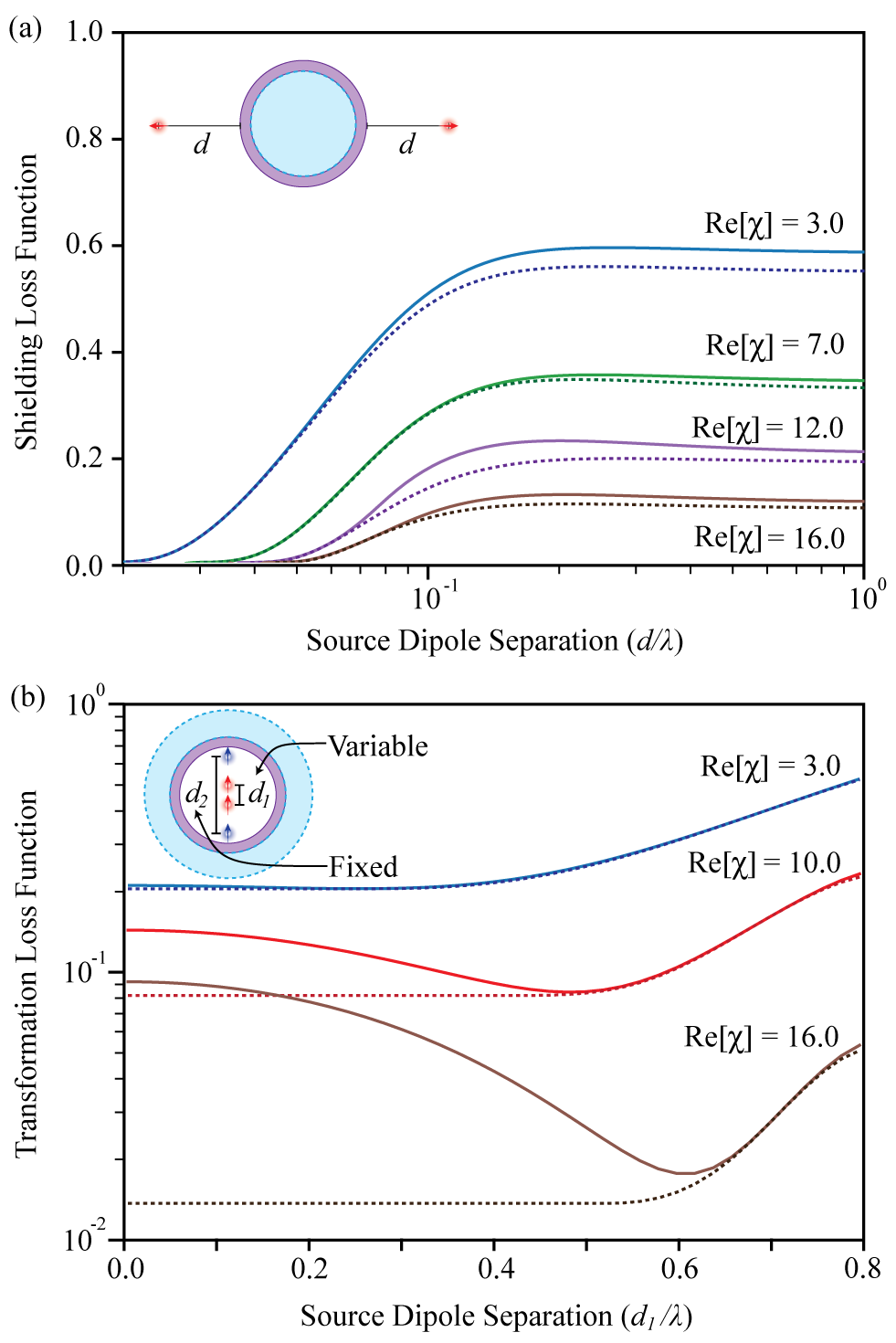
In the limit of large separation, the dipole fields within the design and observation domains closely resemble counter-propagating planewaves. Hence, the constant asymptote value seen as $d$ approaches $\lambda$ is, for all practical purposes, a bound on shielding for two opposing planewaves. The decrease of the bounds for small separation, speculatively, is caused by a combination of localization effects. As the dipoles are brought into the near-field of the design, the bulk of the field magnitude increasingly shifts towards the edge of the observation region. Consequently, inducing small shifts in the position of the field results in a comparatively larger field expulsion. The presence of relatively larger evanescent fields likely also simplifies the suppression of total emission via the (inverse) Purcell effect.

The imposition of cross-constraints (solid lines), which in the limit of point clusters enforce that all considered channels are realized within one common geometry (see Sec. II.3), is seen to produce a relatively small correction to the bounds attained for independently optimized channels (dashed lines). This suggests that although perfect shielding is not possible at sufficiently large dipole separation, given the small shell and material constraints investigated, many structures may potentially achieve similar performance, i.e. the considered channels have yet to “set” the scattering structure in any meaningful way.

Objective—Manipulate the field emanating from a pair of axially aligned dipoles, again limiting the volume available for device design to a thin encompassing spherical shell, so that exterior to the shell it appears that the dipoles are separated by either a larger or smaller distance. If the field is altered so that the separation distance appears larger than it actually is, it is easier to resolve that there are in fact two dipoles present, instead of a single dipole of some effective strength.

More exactly, the input field is generated by a pair of z polarized dipole sources, labeled 1 and 2, situated at $+d_{i}\hat{\textbf{z}}$ and $-d_{i}\hat{\textbf{z}}$ for $i=1,2$, and the target field is taken to arise from equivalent dipolar configuration with a distinct separation, $\pm d_{t}\hat{\textbf{z}}$. The observation domain is set to be a shell of half wavelength thickness enveloping the design domain, which extends from an inner radius of $0.48~\lambda$ to an outer radius of $0.5~\lambda$. Bounds, in all cases, are computed using ten spherical clusters, evenly spanning the design domain with respect to radius. Additional technical details concerning the example are given in Sec. V.1.

The bounds depicted in the three heat maps of Fig. 4, exploring variations in both input $d_{1}=d_{2}$ and output $d_{t}$ pair separations, indicate that the challenge of either reducing or enlarging the perceived separation of the source varies sizably with supposed material properties and gap distances. For larger target or source separations (dipoles approaching the interior surface of the design domain) the increasingly dominant role of evanescent fields makes almost any transformation challenging, especially in weakly polarizable media. Focusing on Fig. 4(b), where the real part of the permittivity is limited to small positive numbers (weak dielectrics), the bounds prove that neither separation manipulation behavior is achievable in any practical sense when the input and target separations vary by more than $\approx 0.25~\lambda$. Conversely, even under the imposition of considerably larger material loss ($\operatorname{Im}\left[\chi\right]$), panel (a) suggests that much better performance is achievable with metals ($\operatorname{Re}\left[\chi\right]<-1$). Intuitively, the subwavelength characteristics of the system do not preclude resonant response in this case since plasmon excitations remain possible. The observed asymmetry between increasing and reducing perceived separation seen in panels (b) and (c), which is largely absent in the metallic example of panel (a), is likely also tied to decaying waves: larger gaps produce larger evanescent fields in the observation domain compared to what is provided by the source, but smaller target separations do not.

Figure 3(b) explores the impact of distinct source separations, varying $d_{1}$ while keeping $d_{2}=0.7~\lambda$ fixed, for a common target field corresponding to two co-located dipoles at the center of the ball, $d_{t}=0$. The findings highlight the need to enforce that performance bounds for multiple channels refer to a unique scattering geometry, achieved via the presence of cross-constraints in the optimization (see Sec. II.3). When the two channels are analyzed separately (dashed lines), the bound values match those displayed on the heat maps of Fig. 4, with the contribution of source 1 to the loss function approaching zero as $d_{1}\to 0$, since in this regime the source and target fields match. However, when cross-constraints are included, the lack of a need for a design in this regime for the first source is at odds with what is needed to convert the field of the widely separated $d_{2}$ source, leading to degraded performance. As $d_{1}$ approaches $d_{2}$, the requirement of a unique gemometry no longer introduces additional requirements, and thus the “simultaneous” (cross-constrained) and “independent” results merge.

Objective—Within a bounding rectangle, design a two-dimensional scattering profile, for a known collection of incident waves, such that the relation between each incident field and total field, along specified input and output observation planes, reproduces the action of Volterra (integration) or differentiation operator. Given that the Volterra and differentiation kernels are two of the basic elements of differential equations, these examples are of considerable interest in relation to recent proposals for optical computing Estakhri et al. 2019, Li et al. 2019, Rajabalipanah et al. 2020.

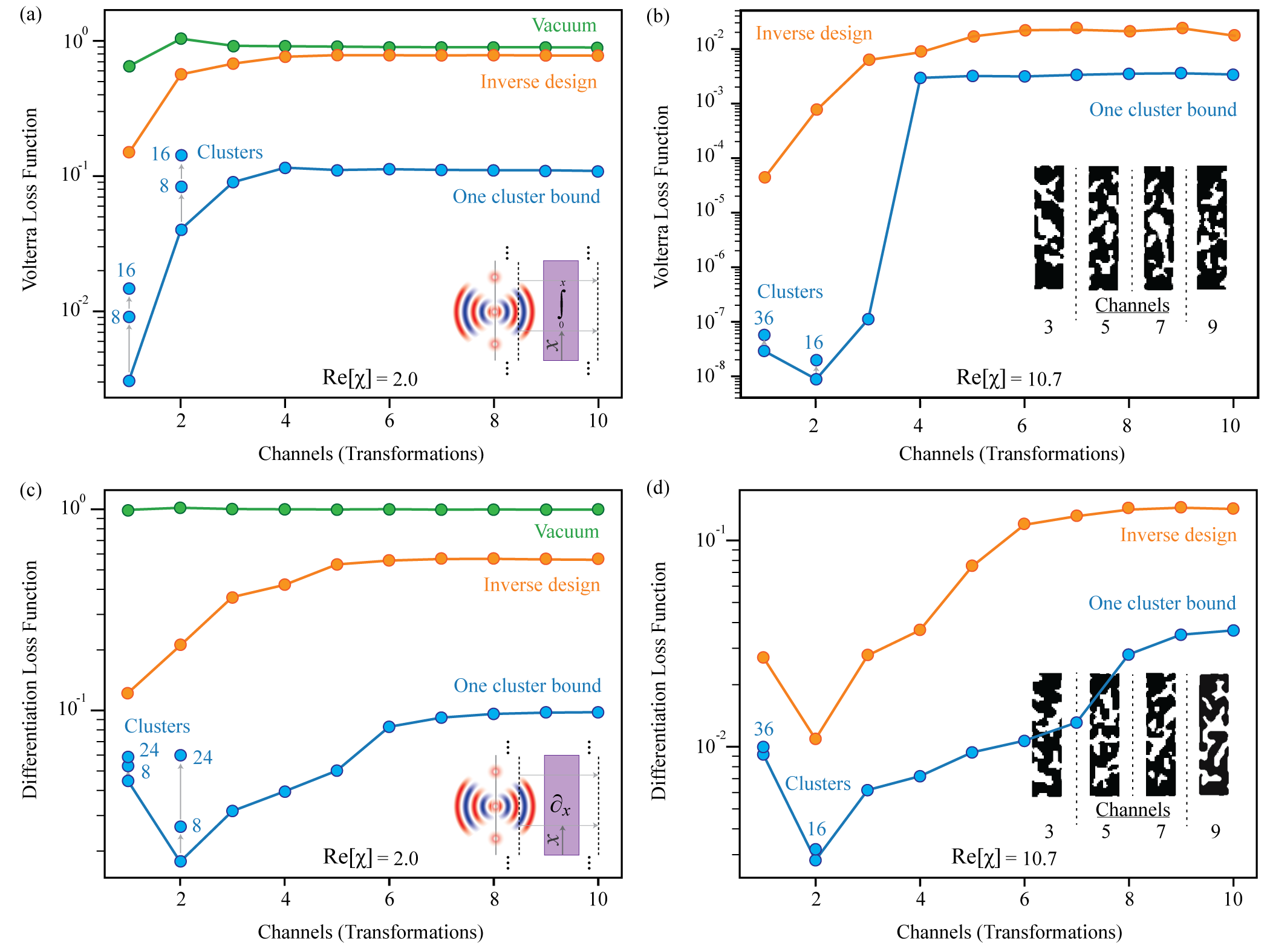
The design region is chosen to have a transverse length (thickness) of $0.5~\lambda$ and parallel length of $2~\lambda$, insets Fig. 5(a) and Fig. 5(c). The input observation plane is set at distance of $0.25~\lambda$ from the input edge of the design region, and the output observation plane is located at a distance of $0.25~\lambda$ from the output edge of the design region. Incident fields are generated by dipole (pixel) sources placed on a source plane, running parallel to the long edge of the design region, situated at a distance $0.2~\lambda$ from the input observation plane. The source plane has length of $1.5~\lambda$ and is centered in relation to the design domain, creating a $0.25~\lambda$ offset from the top and bottom edges of the design region and input and output planes. For the Volterra operator, the target fields along the output plane, letting $y$ denote the direction running parallel to the long edge of the design region, are calculated as $\textbf{E}^{\diamond}\left(x_{\diamond},y\right)=\int^{y}_{0}\text{d}y^{\prime}~\textbf{E}^{i}(x_{i},y^{\prime})$, with $x_{\diamond}$ and $x_{i}$ denoting the common coordinate of the output and input plane, respectively. For the differential operator, keeping the above notation, the target fields are calculated as $\textbf{E}^{\diamond}\left(x_{\diamond},y\right)=\partial\textbf{E}^{i}\left(x_{i},y\right)/\partial y$, implemented as a finite-difference approximation on a computational grid. The optimization objective is defined by Eq. (7) and the bounds formulated following the description given in Sec. II. Further implementation details appear in Sec. V.2. The loss function values appearing in Fig. 5 are determined by

In Eq. (21), $\mathbb{I}_{\text{out}}$ denotes projection onto the output observation plane, and an overline on a vector indicates vertical concatenation over all like named fields indexed by the incident waves, i.e. $\big|\overline{\textbf{E}^{t}}\big>=\left[\big|\textbf{E}^{t}_{1}\big>~,\dots,~\big|\textbf{E}^{t}_{{}_{N}}\big>\right]$ for $N$ sources. The cluster numbers appearing in Fig. 5 refer to specific, even and consistent, divisions of the design domain rectangle along its long and short edges. Writing division of the short edge first, $8=2\times 4$, $16=2\times 8$, $24=3\times 8$ and $36=3\times 12$.

The most striking aspect of the findings displayed in Fig. 5, especially when viewed in conjunction with Fig. 6, is the widely varying characteristics observed between the four cases. For the Volterra and differentiation kernels, at least within the subbasis used here, the number of channels considered has a remarkable influence on the observed limit values. Given that analogous trends are seen in performance of the associated structural optimizations, it can be safely concluded that this behavior is fundamental, hinting that there is a sort of Fourier (resolution) limit at play (e.g., size-dependent constraints on space-bandwidth products are known to limit the degree to which a given optical feature may be resolved with a finite device Mendlovic and Lohmann 1997, Neifeld 1998). Moreover, presumably because differentiation demands creation of more rapid profile variations whereas Volterra operations demand only smoothing, loss function values (for both bounds and inverse design) differ by multiple orders of magnitude for small numbers of channels ($\approx 3$) before reaching “asymptotes” that differ roughly by a factor of $10$, for $\chi=10.7+i~0.01$. Conversely, in the focusing example examined in Fig. 6, the bounds exhibit only a weak dependence on the number of channels in either representative material. While a precise account of the factors leading to these differences is likely challenging, it should be noted that in all cases the objective is bounded (from above or below) by performance that could be achieved in vacuum or a full slab, and so the appearance of plateaus when performance is poor should come as no surprise. A related, albeit more intuitive, dichotomy is seen with respect to the number of clusters imposed and the magnitude of electric susceptibility ($\operatorname{Re}\left[\chi\right]$). For $\operatorname{Re}\left[\chi\right]=2$, subdividing the domain generally leads to substantial tightening, while for $\operatorname{Re}\left[\chi\right]=10$ many more clusters are needed to produce meaningful alterations owing to the decrease in the effective wavelength in the medium.

Objective—Working within a given bounding rectangular design domain, maximize the average field intensity within a specified focal region for a predefined set of incident plane waves spanning a cone of incidence.

The size of the rectangular design region is characterized by the lengths $L_{1}^{d}=0.5~\lambda$ and $L_{2}^{d}=2~\lambda$, inset Fig. 6. The focal region is a square centered along $L_{2}^{d}$, with side length $L_{1}^{f}=L_{2}^{f}=0.25~\lambda$. The middle of the focal region is set to reside at a distance of $0.5~\lambda$ from the outgoing edge of design region. The design objective is

where the summation index runs over the $N$ angles of incidence, evenly distributed over a cone of $(N-1)\times 15^{\circ}$ degrees centered on the midpoint of $L^{2}_{d}$. As before, the cluster labels given in Fig. 6 reference even divisions of the rectangular design domain along its short and long edges: $16=2\times 8$, $32=4\times 8$, $36=3\times 12$, $100=5\times 20$, and $256=8\times 32$.

Even in comparison to previous examples, the extent to which inverse design is able to approach the limit values produced by the formulation of Sec. II is notable. For a single source (a normally incident planewave), agreement within a factor of $3$ is achieved when a single cluster constraint is supposed, and as increasingly localized domain constraints are imposed the performance gap is seen to nearly close. Hence, somewhat surprisingly, the relatively poor field localization values achieved by the topology optimized (inverse design) geometries are in fact not far from ideal. We suspect that three underlying factors are largely responsible for these findings. First, the focusing problem does not impose any specific target profile for the output fields, inset Fig. 6(b), leading to a greater variety of geometric possibilities with similar focusing performance. Second, given the assumed design domain, the specified location and volume of the focal region makes the problem more difficult than what might be naively expected Christiansen and Sigmund 2021; quite different results may be encountered if the “spot size”, or separation between the focus and design domain, are reduced. Third, the extended nature of planewave sources naturally suggests the uniform cluster constraints that have been employed. Contrastingly, for the Volterra and difference kernels, it is plausible that non-uniform cluster distributions, or simply smaller clusters, could lead to tighter bounds. A systematic study of such questions, once a more resource-effective approach for solving Eq. (9) is found Angeris et al. 2021, remains as an important direction for future work.

Following results of Ref. Wittmann 1988, as explained in Refs. Xu 1996, Krüger et al. 2012, off-origin, on-axis, outgoing spherical waves can be expanded in terms of on-origin outgoing and regular spherical waves as

where

In Eqs. (24)–(27), the large round brackets are Wigner-3j symbols, $j_{\nu}$ and $h_{\nu}$ denote the spherical Bessel and Hankel functions of the first kind respectively, and the plus and minus signs indicate the sign of the necessary coordinate transformation. Noting that the field of a $\hat{\textbf{z}}$-polarized dipole radiation consists entirely of the $\textbf{N}_{1,0}$ outgoing wave,

the field of an off-axis dipole can thus be computed from Eqs. (24)–(27) by setting $p=N,~l=1,$ and $m=0$ implying, through the Wigner selection rules that the on-origin regular $M$ waves, RgM, waves need not be included. Using this knowledge, the expansion coefficients for an off-origin, on-axis, dipole can be reduce to

where

$\mathcal{U}^{\text{out}-}_{NN,l,1,0}$ and $\mathcal{U}^{\text{out}+}_{NN,l,1,0}$ are equivalently defined but with the Hankel functions of the first kind, $h_{\nu}\left(dk_{o}\right)$, replaced by Bessel functions of the first kind. In these expressions, summation limits are set by explicit evaluation of the Wigner-3j selection rules and

The Green’s function representations used for computing bounds in all two-dimensional examples were obtained by the open-source ceviche FDFD package Hughes et al. 2019b. The basis used for representing fields in all such cases are the individual discretization pixels of the FDFD computation. Correspondingly, the matrix representation of the Green’s function connects every pixel with a numeric approximation of the field generated by a dipole source at the location of the pixel.

For all studies with a free space background, the translational invariance of the Maxwell is exploited to construct the matrix representation of the Green’s function from a single dipole field solve. Concretely, consider a domain of shape $(N_{x},N_{y})$ in pixels. The required representation of $\mathbb{G}^{0}$ is then a square matrix of dimension $N_{x}N_{y}$, where the $j$-th column is the field created by an electric dipole at position $j$. This matrix can be obtained in a single solve by placing a dipole at the center of a larger $(2N_{x}-1,2N_{y}-1)$ domain and observing the calculated field in sliding a window of size $(N_{x},N_{y})$.

To account for the cross-source constraints in the presence of multiple sources, compared to the approaches we have used in prior works Molesky et al. 2020c, the fields and matrices for each of the individual sources are grouped into “super” vectors and matrices:

As such, the dimension of the vectors and matrices involved in the calculation of a $N$-source bound scales linearly with $N$. To facilitate computation of bounds for large device footprints and values of $N$, an Arnoldi basis for $\mathbb{U}$ is computed to more efficiently represent the $\left|\textbf{T}\right>$ image field. For any given problem, the only vectors that interact with the primal degrees of freedom, $\left\{\big|\textbf{T}_{n}\big>\right\}$, are the sources, $\left\{\big|\textbf{E}^{i}_{n}\big>\right\}$, and the linear coefficients of $\left\{\big|\textbf{T}_{n}\big>\right\}$ in the primal objective $\left\{\big|\mathcal{O}^{\text{lin}}_{n}\big>\right\}$. Hence, these vectors

posses favorable convergence characteristic for computing the dual via Arnoldi iterations. For communications type problems $\big|\mathcal{O}^{\text{lin}}_{n}\big>=\mathbb{G}_{od}^{\dagger}\left(\big|\textbf{E}^{\diamond}_{n}\big>-\big|\textbf{E}^{i}_{n}\big>\right)$, while for the metalens problem $\big|\mathcal{O}^{\text{lin}}_{n}\big>=\mathbb{G}_{od}^{\dagger}\big|\textbf{E}^{i}_{n}\big>$. To begin the Arnoldi procedure, $B_{0}$ is orthonormalized to give $\bar{B}_{0}$. The $i$-th iteration is then computed by generating $B_{i}=\mathbb{U}\bar{B}_{i-1}$, and then orthonormalizing $B_{i}$ both internally and with respect to $\bar{B}_{0},\dots,\bar{B}_{i-1}$, giving $\bar{B}_{i}$. The partial basis for the generated block Krylov subspace at the end of the $i$-th iteration is the thus the aggregate of all the column vectors of $\bar{B}_{0},\dots,\bar{B}_{i}$. Denoting $\mathbb{U}$ restricted to the $i$-th Krylov subspace as $\mathbb{U}_{i}$, the representation is effectively complete when the column norms of $\mathbb{U}_{i}^{-1}\bar{B}_{0}$ converge to within a certain tolerance, Ref. Molesky et al. 2020a.

Inverse design results for all two dimensional examples are also computed using ceviche using a standard topology optimization Christiansen and Sigmund 2021. For sake of comparison with the optimization problem underlying the bound formulation, grayscale structures are treated as viable. That is, in any particular design, the permittivity value of a given pixel can take any value in the convex set bounded by $0$ and the quoted material value.

References

- Verdu [1998] Sergio Verdu. Fifty years of Shannon theory. IEEE Transactions on information theory, 44(6):2057–2078, 1998.
- Robitaille [2009] Pierre-Marie Robitaille. Kirchhoff’s law of thermal emission: 150 years. Progress in Physics, 4:3–13, 2009.
- Shannon [1948] Claude E Shannon. A mathematical theory of communication. The Bell System Technical Journal, 27(3):379–423, 1948.
- Pendry [1983] John Brian Pendry. Quantum limits to the flow of information and entropy. Journal of Physics A: Mathematical and General, 16(10):2161, 1983.
- Caves and Drummond [1994] Carlton M Caves and Peter D Drummond. Quantum limits on bosonic communication rates. Reviews of Modern Physics, 66(2):481, 1994.
- Horodecki et al. [2000] Michał Horodecki, Paweł Horodecki, and Ryszard Horodecki. Limits for entanglement measures. Physical Review Letters, 84(9):2014, 2000.
- Pirandola et al. [2017] Stefano Pirandola, Riccardo Laurenza, Carlo Ottaviani, and Leonardo Banchi. Fundamental limits of repeaterless quantum communications. Nature communications, 8(1):1–15, 2017.
- Miller [2019] David AB Miller. Waves, modes, communications, and optics: a tutorial. Advances in Optics and Photonics, 11(3):679–825, 2019.
- Yablonovitch [1982] Eli Yablonovitch. Statistical ray optics. Journal of the Optical Society of America, 72(7):899–907, 1982.
- Callahan et al. [2012] Dennis M Callahan, Jeremy N Munday, and Harry A Atwater. Solar cell light trapping beyond the ray optic limit. Nano letters, 12(1):214–218, 2012.
- Miroshnichenko and Tribelsky [2018] Andrey E Miroshnichenko and Michael I Tribelsky. Ultimate absorption in light scattering by a finite obstacle. Physical Review Letters, 120(3):033902, 2018.
- Hashemi et al. [2010] Hila Hashemi, Baile Zhang, John D Joannopoulos, and Steven G Johnson. Delay-bandwidth and delay-loss limitations for cloaking of large objects. Physical Review Letters, 104(25):253903, 2010.
- Monticone and Alù [2016] Francesco Monticone and Andrea Alù. Invisibility exposed: physical bounds on passive cloaking. Optica, 3(7):718–724, 2016.
- Cassier and Milton [2017] Maxence Cassier and Graeme W Milton. Bounds on herglotz functions and fundamental limits of broadband passive quasistatic cloaking. Journal of Mathematical Physics, 58(7):071504, 2017.
- Caulfield and Hirschfeld [1977] H. John Caulfield and Tomas Hirschfeld. Optical communication at the source bandwidth limit. Applied Optics, 16(5):1184–1186, 1977.
- Tsakmakidis et al. [2017] Kosmas L Tsakmakidis, Linfang Shen, Sebastian A Schulz, Xiaodong Zheng, John Upham, Xiaohua Deng, Hatice Altug, Alexander F Vakakis, and Robert W Boyd. Breaking lorentz reciprocity to overcome the time-bandwidth limit in physics and engineering. Science, 356(6344):1260–1264, 2017.
- Mann et al. [2019] Sander A Mann, Dimitrios L Sounas, and Andrea Alù. Nonreciprocal cavities and the time–bandwidth limit. Optica, 6(1):104–110, 2019.
- Abu-Mostafa and Psaltis [1987] Yaser S Abu-Mostafa and Demetri Psaltis. Optical neural computers. Scientific American, 256(3):88–95, 1987.
- Hughes et al. [2019a] Tyler W Hughes, Ian AD Williamson, Momchil Minkov, and Shanhui Fan. Wave physics as an analog recurrent neural network. Science advances, 5(12):eaay6946, 2019a.
- Zuo et al. [2019] Ying Zuo, Bohan Li, Yujun Zhao, Yue Jiang, You-Chiuan Chen, Peng Chen, Gyu-Boong Jo, Junwei Liu, and Shengwang Du. All-optical neural network with nonlinear activation functions. Optica, 6(9):1132–1137, 2019.
- Bogaerts et al. [2020] Wim Bogaerts, Daniel Pérez, José Capmany, David AB Miller, Joyce Poon, Dirk Englund, Francesco Morichetti, and Andrea Melloni. Programmable photonic circuits. Nature, 586(7828):207–216, 2020.
- Richardson et al. [2013] David J Richardson, John M Fini, and Lynn E Nelson. Space-division multiplexing in optical fibres. Nature Photonics, 7(5):354–362, 2013.
- Li et al. [2017] Juhao Li, Fang Ren, Tao Hu, Zhengbin Li, Yongqi He, Zhangyuan Chen, Qi Mo, and Guifang Li. Recent progress in mode-division multiplexed passive optical networks with low modal crosstalk. Optical Fiber Technology, 35:28–36, 2017.
- Yang et al. [2020] Zhenshan Yang, Xiaoguang Zhang, Bin Zhang, Xia Zhang, Zhentao Zhang, Xiangguo Meng, and Chenglin Bai. Density-matrix formalism for modal coupling and dispersion in mode-division multiplexing communications systems. Optics Express, 28(13):18658–18680, 2020.
- Estakhri et al. [2019] Nasim Mohammadi Estakhri, Brian Edwards, and Nader Engheta. Inverse-designed metastructures that solve equations. Science, 363(6433):1333–1338, 2019.
- Li et al. [2019] Lianlin Li, Ya Shuang, Qian Ma, Haoyang Li, Hanting Zhao, Menglin Wei, Che Liu, Chenglong Hao, Cheng-Wei Qiu, and Tie Jun Cui. Intelligent metasurface imager and recognizer. Light: Science & Applications, 8(1):1–9, 2019.
- Rajabalipanah et al. [2020] Hamid Rajabalipanah, Ali Abdolali, Shahid Iqbal, Lei Zhang, and Tie Jun Cui. How do space-time digital metasurfaces serve to perform analog signal processing? arXiv:2002.06773, 2020.
- Giovannetti et al. [2009] Vittorio Giovannetti, Seth Lloyd, Lorenzo Maccone, and Jeffrey H Shapiro. Sub-rayleigh-diffraction-bound quantum imaging. Physical Review A, 79(1):013827, 2009.
- Molesky et al. [2020a] Sean Molesky, Pengning Chao, Weiliang Jin, and Alejandro W Rodriguez. Global -operator bounds on electromagnetic scattering: Upper bounds on far-field cross sections. Physical Review Research, 2(3):033172, 2020a.
- Miller et al. [2015] Owen D Miller, Steven G Johnson, and Alejandro W Rodriguez. Shape-independent limits to near-field radiative heat transfer. Physical Review Letters, 115(20):204302, 2015.
- Jin et al. [2019] Weiliang Jin, Sean Molesky, Zin Lin, and Alejandro W Rodriguez. Material scaling and frequency-selective enhancement of near-field radiative heat transfer for lossy metals in two dimensions via inverse design. Physical Review B, 99(4):041403(R), 2019.
- Venkataram et al. [2020a] Prashanth S Venkataram, Sean Molesky, Weiliang Jin, and Alejandro W Rodriguez. Fundamental limits to radiative heat transfer: the limited role of nanostructuring in the near-field. Physical Review Letters, 124(1):013904, 2020a.
- Piggott et al. [2014] Alexander Y Piggott, Jesse Lu, Thomas M Babinec, Konstantinos G Lagoudakis, Jan Petykiewicz, and Jelena Vučković. Inverse design and implementation of a wavelength demultiplexing grating coupler. Scientific Reports, 4(1):1–5, 2014.
- Michaels and Yablonovitch [2018] Andrew Michaels and Eli Yablonovitch. Inverse design of near unity efficiency perfectly vertical grating couplers. Optics express, 26(4):4766–4779, 2018.
- Yang et al. [2018] Jianji Yang, David Sell, and Jonathan A Fan. Freeform metagratings based on complex light scattering dynamics for extreme, high efficiency beam steering. Annalen der Physik, 530(1):1700302, 2018.
- Thureja et al. [2020] Prachi Thureja, Ghazaleh Kafaie Shirmanesh, Katherine T Fountaine, Ruzan Sokhoyan, Meir Grajower, and Harry A Atwater. Array-level inverse design of beam steering active metasurfaces. ACS Nano, 2020.
- Akgol et al. [2018] Oguzhan Akgol, Emin Unal, Olcay Altintas, Muharrem Karaaslan, Faruk Karadag, and Cumali Sabah. Design of metasurface polarization converter from linearly polarized signal to circularly polarized signal. Optik, 161:12–19, 2018.
- Chung and Miller [2020] Haejun Chung and Owen D Miller. High-na achromatic metalenses by inverse design. Optics Express, 28(5):6945–6965, 2020.
- Lu and Vučković [2010] Jesse Lu and Jelena Vučković. Inverse design of nanophotonic structures using complementary convex optimization. Optics Express, 18(4):3793–3804, 2010.
- Lu and Vučković [2012] Jesse Lu and Jelena Vučković. Objective-first design of high-efficiency, small-footprint couplers between arbitrary nanophotonic waveguide modes. Optics express, 20(7):7221–7236, 2012.
- Miller et al. [2016] Owen D Miller, Athanasios G Polimeridis, M. T. Homer Reid, Chia Wei Hsu, Brendan G DeLacy, John D Joannopoulos, Marin Soljačić, and Steven G Johnson. Fundamental limits to optical response in absorptive systems. Optics Express, 24(4):3329–3364, 2016.
- Angeris et al. [2019] Guillermo Angeris, Jelena Vučković, and Stephen P Boyd. Computational bounds for photonic design. ACS Photonics, 6(5):1232, 2019. doi:10.1021/acsphotonics.9b00154.
- Molesky et al. [2019] Sean Molesky, Weiliang Jin, Prashanth S Venkataram, and Alejandro W Rodriguez. -operator bounds on angle-integrated absorption and thermal radiation for arbitrary objects. Physical Review Letters, 123:257401, 2019.
- Molesky et al. [2020b] Sean Molesky, Prashanth S Venkataram, Weiliang Jin, and Alejandro W Rodriguez. Fundamental limits to radiative heat transfer: theory. Physical Review B, 101(3):035408, 2020b.
- Molesky et al. [2020c] Sean Molesky, Pengning Chao, and Alejandro W Rodriguez. Hierarchical mean-field -operator bounds on electromagnetic scattering: Upper bounds on near-field radiative purcell enhancement. Physical Review Research, 2(4):043398, 2020c.
- Gustafsson et al. [2020] Mats Gustafsson, Kurt Schab, Lukas Jelinek, and Miloslav Capek. Upper bounds on absorption and scattering. New Journal of Physics, 2020.
- Venkataram et al. [2020b] Prashanth S Venkataram, Sean Molesky, Pengning Chao, and Alejandro W Rodriguez. Fundamental limits to attractive and repulsive casimir-polder forces. Physical Review A, 101(5):052115, 2020b.
- Kuang et al. [2020] Zeyu Kuang, Lang Zhang, and Owen D Miller. Maximal single-frequency electromagnetic response. arXiv:2002.00521, 2020.
- Schab et al. [2020] Kurt Schab, Austin Rothschild, Kristi Nguyen, Miloslav Capek, Lukas Jelinek, and Mats Gustafsson. Trade-offs in absorption and scattering by nanophotonic structures. Optics Express, 28(24):36584–36599, 2020.
- Trivedi et al. [2020] Rahul Trivedi, Guillermo Angeris, Logan Su, Stephen Boyd, Shanhui Fan, and Jelena Vuckovic. Fundamental bounds for scattering from absorptionless electromagnetic structures. arXiv:2003.00374, 2020.
- Kuang and Miller [2020] Zeyu Kuang and Owen D Miller. Computational bounds to light-matter interactions via local conservation laws. arXiv preprint arXiv:2008.13325, 2020.
- [52] L Jelinek, M Gustafsson, M Capek, and K Schab. Sub-structure limits to optical phenomena. In 2020 Fourteenth International Congress on Artificial Materials for Novel Wave Phenomena (Metamaterials), pages 400–402. IEEE.
- Angeris et al. [2021] Guillermo Angeris, Jelena Vučković, and Stephen Boyd. Heuristic methods and performance bounds for photonic design. Optics Express, 29(2):2827–2854, 2021.
- Rudin [2006] Walter Rudin. Real and complex analysis. Tata McGraw-hill education, 2006.
- Miller [2012] David AB Miller. All linear optical devices are mode converters. Optics express, 20(21):23985–23993, 2012.
- Miller [2013a] David AB Miller. Self-configuring universal linear optical component. Photonics Research, 1(1):1–15, 2013a.
- Miller et al. [2017] David AB Miller, Linxiao Zhu, and Shanhui Fan. Universal modal radiation laws for all thermal emitters. Proceedings of the National Academy of Sciences, 114(17):4336–4341, 2017.
- Pai et al. [2019] Sunil Pai, Ben Bartlett, Olav Solgaard, and David AB Miller. Matrix optimization on universal unitary photonic devices. Physical Review Applied, 11(6):064044, 2019.
- Miller [2007] David A B Miller. Fundamental limit for optical components. Journal of the Optical Society of America B, 24(10):A1–A18, 2007.
- Miller [2013b] David AB Miller. How complicated must an optical component be? JOSA A, 30(2):238–251, 2013b.
- Tsang et al. [2004] Leung Tsang, Jin Au Kong, and Kung-Hau Ding. Scattering of electromagnetic waves: Theories and applications, volume 27. John Wiley & Sons, 2004.
- Kirsch and Lechleiter [2009] Andreas Kirsch and Armin Lechleiter. The operator equations of Lippmann–Schwinger type for acoustic and electromagnetic scattering problems in L2. Applicable Analysis, 88(6):807–830, 2009.
- Costabel et al. [2012] Martin Costabel, Eric Darrigrand, and Hamdi Sakly. The essential spectrum of the volume integral operator in electromagnetic scattering by a homogeneous body. 2012.
- Krüger et al. [2012] Matthias Krüger, Giuseppe Bimonte, Thorsten Emig, and Mehran Kardar. Trace formulas for nonequilibrium casimir interactions, heat radiation, and heat transfer for arbitrary objects. Physical Review B, 86(11):115423, 2012.
- Colton and Kress [2019] David Colton and Rainer Kress. Inverse acoustic and electromagnetic scattering theory, volume 93. Springer Nature, 2019.
- [66] Note1. All operators and fields are supposed to be frequency dependent, and every stated relation holds at any given frequency.
- [67] Note2. The potential of the scatterer is constructed via the explicit spatial projection operator , which is defined to be identity at spatial locations within the scatterer and zero at all other points in the domain , and the implicit spatial projection into the scattering object encoded in the definition the scattering operator, .
- [68] Note3. The specification of an initial field is essentially equivalent to the introduction of a source, or flux boundary condition, in Maxwell’s equations.
- Liu et al. [2017] Jingfeng Liu, Ming Zhou, Lei Ying, Xuewen Chen, and Zongfu Yu. Enhancing the optical cross section of quantum antenna. Physical Review A, 95(1):013814, 2017.
- Koenderink [2017] A Femius Koenderink. Single-photon nanoantennas. ACS Photonics, 4(4):710–722, 2017.
- Cox et al. [2018] Kevin C Cox, David H Meyer, Fredrik K Fatemi, and Paul D Kunz. Quantum-limited atomic receiver in the electrically small regime. Physical Review Letters, 121(11):110502, 2018.
- Mokkapati and Catchpole [2012] Sudha Mokkapati and KR Catchpole. Nanophotonic light trapping in solar cells. Journal of Applied Physics, 112(10):101101, 2012.
- Sheng et al. [2012] Xing Sheng, Juejun Hu, Jurgen Michel, and Lionel C Kimerling. Light trapping limits in plasmonic solar cells: an analytical investigation. Optics Express, 20(104):A496–A501, 2012.
- Ganapati et al. [2013] Vidya Ganapati, Owen D Miller, and Eli Yablonovitch. Light trapping textures designed by electromagnetic optimization for subwavelength thick solar cells. IEEE Journal of Photovoltaics, 4(1):175–182, 2013.
- Phan-huy Hao [1982] E Phan-huy Hao. Quadratically constrained quadratic programming: Some applications and a method for solution. Zeitschrift für Operations Research, 26(1):105–119, 1982.
- Bose et al. [2015] Subhonmesh Bose, Dennice F Gayme, K Mani Chandy, and Steven H Low. Quadratically constrained quadratic programs on acyclic graphs with application to power flow. IEEE Transactions on Control of Network Systems, 2(3):278–287, 2015.
- [77] Note4. Technically, should be complete, and hence infinite dimensional. In practice, however, must truncated to some finite set in order to apply numerical methods. A similar approximation is needed in any numeric solver for electromagnetics.
- Park and Boyd [2017] Jaehyun Park and Stephen Boyd. General heuristics for nonconvex quadratically constrained quadratic programming. arXiv:1703.07870, 2017.
- Boyd and Vandenberghe [2004] Stephen Boyd and Lieven Vandenberghe. Convex optimization. Cambridge university press, 2004.
- [80] Note5. Cluster refinements, as shown in Ref. Molesky et al. 2020c, can be given a mathematical ordering that is preserved in the limit values obtained in the associated optimization, whether or not the dual is used to relax the optimization.
- [81] Note6. In particular, if , so that there is only a single cluster filling the entire domain, then the symmetric () and antisymmetric () parts of the scattering constraints impose that both real and reactive power must be conserved, as was studied in Refs. Molesky et al. 2019, Gustafsson et al. 2020.
- Plefka [1982] Timm Plefka. Convergence condition of the tap equation for the infinite-ranged ising spin glass model. Journal of Physics A, 15(6):1971, 1982.
- Jin et al. [2016] Jiasen Jin, Alberto Biella, Oscar Viyuela, Leonardo Mazza, Jonathan Keeling, Rosario Fazio, and Davide Rossini. Cluster mean-field approach to the steady-state phase diagram of dissipative spin systems. Physical Review X, 6(3):031011, 2016.
- Nourian and Caines [2013] Mojtaba Nourian and Peter E Caines. -nash mean field game theory for nonlinear stochastic dynamical systems with major and minor agents. SIAM Journal on Control and Optimization, 51(4):3302–3331, 2013.
- Şen and Caines [2016] Nevroz Şen and Peter E Caines. Mean field game theory with a partially observed major agent. SIAM Journal on Control and Optimization, 54(6):3174–3224, 2016.
- Kappen and Ortiz [1998] Hilbert J Kappen and Francisco de Borja Rodríguez Ortiz. Boltzmann machine learning using mean field theory and linear response correction. In Advances in Neural Information Processing Systems, pages 280–286, 1998.
- Chen et al. [2018] Minmin Chen, Jeffrey Pennington, and Samuel S Schoenholz. Dynamical isometry and a mean field theory of rnns: Gating enables signal propagation in recurrent neural networks. arXiv:1806.05394, 2018.
- [88] Note7. Duality can also be used to solve a relaxation of the mean-field optimization that in many cases is in fact a true solution Boyd and Vandenberghe 2004.
- Mendlovic and Lohmann [1997] David Mendlovic and Adolf W Lohmann. Space–bandwidth product adaptation and its application to superresolution: fundamentals. JOSA A, 14(3):558–562, 1997.
- Neifeld [1998] Mark A Neifeld. Information, resolution, and space–bandwidth product. Optics Letters, 23(18):1477–1479, 1998.
- Christiansen and Sigmund [2021] Rasmus E Christiansen and Ole Sigmund. Inverse design in photonics by topology optimization: tutorial. JOSA B, 38(2):496–509, 2021.
- Kruk and Kivshar [2017] Sergey Kruk and Yuri Kivshar. Functional meta-optics and nanophotonics governed by mie resonances. ACS Photonics, 4(11):2638–2649, 2017.
- Lewi et al. [2019] Tomer Lewi, Nikita A Butakov, Hayden A Evans, Mark W Knight, Prasad P Iyer, David Higgs, Hamid Chorsi, Juan Trastoy, Javier Del Valle Granda, Ilya Valmianski, et al. Thermally reconfigurable meta-optics. IEEE Photonics Journal, 11(2):1–16, 2019.
- Staude et al. [2019] Isabelle Staude, Thomas Pertsch, and Yuri S Kivshar. All-dielectric resonant meta-optics lightens up. ACS Photonics, 6(4):802–814, 2019.
- Lin et al. [2020] Zin Lin, Charles Roques-Carmes, Raphaël Pestourie, Marin Soljačić, Arka Majumdar, and Steven G Johnson. End-to-end inverse design for inverse scattering via freeform metastructures. arXiv:2006.09145, 2020.
- Schneider et al. [2018] Philipp-Immanuel Schneider, Nicole Srocka, Sven Rodt, Lin Zschiedrich, Stephan Reitzenstein, and Sven Burger. Numerical optimization of the extraction efficiency of a quantum-dot based single-photon emitter into a single-mode fiber. Optics Express, 26(7):8479–8492, 2018.
- Shen et al. [2020] Lian Shen, Xiao Lin, Mikhail Y Shalaginov, Tony Low, Xianmin Zhang, Baile Zhang, and Hongsheng Chen. Broadband enhancement of on-chip single-photon extraction via tilted hyperbolic metamaterials. Applied Physics Reviews, 7(2):021403, 2020.
- Wambold et al. [2021] Raymond A Wambold, Zhaoning Yu, Yuzhe Xiao, Benjamin Bachman, Gabriel Jaffe, Shimon Kolkowitz, Jennifer T Choy, Mark A Eriksson, Robert J Hamers, and Mikhail A Kats. Adjoint-optimized nanoscale light extractor for nitrogen-vacancy centers in diamond. Nanophotonics, 10(1):393–401, 2021.
- Chakravarthi et al. [2020] Srivatsa Chakravarthi, Pengning Chao, Christian Pederson, Sean Molesky, Karine Hestroffer, Fariba Hatami, Alejandro W Rodriguez, and Kai-Mei C Fu. Inverse-designed photon extractors for optically addressable defect qubits. arXiv:2007.12344, 2020.
- [100] Note8. It should be mentioned that we have encountered situations in which very high numeric precision was required to verify the presence of strong duality.
- Valmadre et al. [2017] Jack Valmadre, Luca Bertinetto, Joao Henriques, Andrea Vedaldi, and Philip HS Torr. End-to-end representation learning for correlation filter based tracking. In Proceedings of the IEEE Conference on Computer Vision and Pattern Recognition, pages 2805–2813, 2017.
- Poyneer and Véran [2005] Lisa A Poyneer and Jean-Pierre Véran. Optimal modal fourier-transform wavefront control. JOSA A, 22(8):1515–1526, 2005.
- Sitzmann et al. [2018] Vincent Sitzmann, Steven Diamond, Yifan Peng, Xiong Dun, Stephen Boyd, Wolfgang Heidrich, Felix Heide, and Gordon Wetzstein. End-to-end optimization of optics and image processing for achromatic extended depth of field and super-resolution imaging. ACM Transactions on Graphics (TOG), 37(4):1–13, 2018.
- Wittmann [1988] Ronald C Wittmann. Spherical wave operators and the translation formulas. IEEE Transactions on Antennas and Propagation, 36(8):1078–1087, 1988.
- Xu [1996] Yu-lin Xu. Calculation of the addition coefficients in electromagnetic multisphere-scattering theory. Journal of Computational Physics, 127(2):285–298, 1996.
- Hughes et al. [2019b] Tyler W Hughes, Ian AD Williamson, Momchil Minkov, and Shanhui Fan. Forward-mode differentiation of maxwell’s equations. ACS Photonics, 6(11):3010–3016, 2019b.