The role of viscous regularization in dynamical problems, strain localization and mesh dependency Journal: Computer Methods in Applied Mechanics and Engineering

Let us consider a body under homogeneous small deformation lying at rest. The equilibrium equation is given as:

where $\sigma^{\star}_{ij}$ is the developed stress field, $i,j$ are indices indicating the directions of the components of the stress field $(i,j=1...3)$. In the above relation ($,j$) indicates the partial spatial derivative with respect to the $j$ direction. The Einstein summation condition over repeated indices is implied. Considering a perturbation $\tilde{u}_{i}$ to the reference displacement field $u^{\star}_{i}$ of homogeneous deformation, we find a relationship between the perturbed stress and displacement $\tilde{u}$ fields, according to the conservation of linear momentum:

where $(\cdot)$ corresponds to the time derivative and $\rho$ is the density of the material. Both displacement and stress variations are arbitrary respecting only the boundary and loading conditions such that $\tilde{u}_{i}=0,\tilde{\sigma}_{i,j}n_{j}=0$ at the boundary of the body, where displacement and loading conditions are specified, respectively. In order to continue with the bifurcation analysis of the problem we need to look first at the elasto-viscoplastic constitutive law we take into account.

We proceed now in deriving the general linearized perturbed equation of equilibrium for the given material law under monotonic loading. Inserting equation (11) into equation (3) and taking into account the spatial derivative of equation (7), we obtain:

This equation describes the spatio-temporal evolution of perturbations from the reference solution of homogeneous deformation in 3D.

Equation (19) consists of two multivalued functions $\bar{k}_{1}(\bar{\omega}),\bar{k}_{2}(\bar{\omega})$ in the complex set $\bar{\omega}\;\in\;\mathbb{C}$. Introduction of branch cuts along selected points of unambiguous value is needed for their study on the values of their argument $\bar{\omega}$ Arfken and Weber 1999.
Noticing the square powers of $V^{2},\;\bar{\omega}^{2}$ inside the root, equation (19) can be simplified yielding:

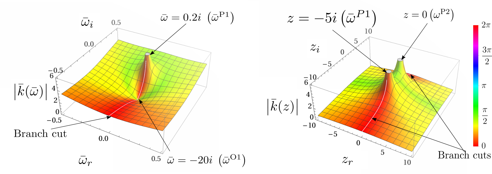
Each of the two solutions contains right and left propagating waves based on the sign combinations of $\bar{\omega}_{r},\bar{k}_{r}$. The second solution $\bar{k}_{2}(\omega)$ presents the exact same points of interest as the first. The difference lies in the $-1$ factor between the two solutions. This factor according to the Euler identity can be written as $e^{i\pi}=-1$ and ,therefore, indicates a change in the argument of the second solution. Figure 1 shows 3D plots of $\bar{k}_{1}(\bar{\omega}),\;\bar{k}_{2}(\bar{\omega})$. The colors on the right of Figure 1 are changed indicating a change of the argument from the upper half of the imaginary plane to the lower half of it, meaning that the two solutions $\bar{k}_{1,2}(\bar{\omega})$ behave differently when it comes to the spatial amplification/attenuation coefficient $\bar{k}_{i}$. In particular, $\bar{k}_{1}(\bar{\omega})$ predicts only attenuation waves, while $\bar{k}_{2}(\bar{\omega})$ consists of amplification waves. This change indicates that the waves in Figure 1 travel in the same direction with opposite imaginary part of $\bar{k}(\bar{\omega})$. To us the propagation direction of the wave is not important because of spatial symmetry of the solution (19).

In the next section the points of interest of the $\bar{k}_{1}(\bar{\omega})$ are presented and their behavior is explained in the form of branch cuts and poles. As discussed previously, the same behavior is valid for $\bar{k}_{2}(\bar{\omega})$. We choose to draw further conclusions in the form of plots over line from the combination of the two solutions $\bar{k}_{1,2}(\bar{\omega})$. In particular, we focus on the positive real parts of the solutions $\bar{k}_{1r}(\bar{\omega}),\bar{k}_{2r}(\bar{\omega})>0$ as well as the positive imaginary parts of the solutions $\bar{k}_{1i}(\bar{\omega}),\bar{k}_{2i}(\bar{\omega})>0$. Thus, we investigate the function $\bar{k}{(\omega)}=|\bar{k}_{r}(\bar{\omega})|+i|\bar{k}_{i}(\bar{\omega})|$ as shown later in Figure 4.

Studying equation (23), the following points can be readily specified in the above form:

• 1.

  The third factor indicates a zero at the origin: $\bar{\omega}^{\text{O1}}=0$.

• 2.

  The fourth factor becomes zero at position: $\bar{\omega}^{\text{O2}}=-\frac{3+\bar{h}}{T}i$.

• 3.

  The last factor indicates the presence of a pole at: $\bar{\omega}^{\text{P1}}=-\frac{\bar{h}}{T}i$.

• 4.

  The value of the function at complex infinity $\bar{\omega}^{\text{P2}}\rightarrow\infty$ is found to be infinite in a complex sense, $\lim_{\bar{\omega}\rightarrow\bar{\omega}^{\text{P2}}}\bar{k}_{1}(\bar{\omega})\rightarrow\infty$.

For the purposes of our analysis the behavior of the dispersion function at the poles $\bar{\omega}^{\text{P1}},\;\bar{\omega}^{\text{P2}}$ is very important as it will be shown to promote localization on a mathematical plane.

Because of the fractional powers of the second and third term, equation (23) is a multivalued equation, since it is affected by the values of the argument. In order to remove the ambiguity from the function we need to constrain it in such a way that each value of the function corresponds to only one argument. For this we introduce branch cuts. A branch cut is a discontinuity in the function that is defined by arbitrarily joining the two points defined as branch points. The branch points are defined as points of unambiguous value, where the argument of the function is exactly known for a particular value of the function and the values corresponding to other points in a region sufficiently close to the branch point depends on the argument of the complex number inserted in the function. Two such points for the complex function $f(\bar{\omega})=\bar{\omega}^{\frac{1}{2}}$ are $\bar{\omega}=0,\;\text{and}\;|\bar{\omega}|\rightarrow\infty,\;\bar{\omega}\in\mathbb{C}$, because for these particular numbers the value of the function is always zero and infinity respectively. However, around them the value of the function depends on the argument of the complex number (see below).

We can translate this result to other points in the complex plane, namely to $\bar{\omega}^{\text{O2}},\;\bar{\omega}^{\text{P1}}$. In a region close and around $\bar{\omega}^{\text{O2}}=-i\frac{3+\bar{h}}{T}$ the complex number with starting point $\bar{\omega}^{\text{O2}}$ that follows the curve surrounding $\bar{\omega}^{\text{O2}}$ changes its argument by $2\pi i$. However, the factor $\left(\frac{3+\bar{h}}{iT}-\bar{\omega}\right)^{\frac{1}{2}}$ only changes by $\pi i$, meaning that there is a sign difference between the starting and the end position along the closed curve at the same point. Similarly, the same happens in the region near the pole $\bar{\omega}^{\text{P1}}$, where for every $2\pi i$ that the relative complex number starting at $\bar{\omega}^{\text{P1}}$ changes following the surrounding curve, the factor $\left(\frac{\bar{h}}{iT}-\bar{\omega}\right)^{-\frac{1}{2}}$ changes by $-\pi i$. However at complex infinity $(\bar{\omega}\rightarrow\infty)$, both previous points are entailed by the curve at infinity. Therefore, the total change in the argument is $\pi i-\pi i=0$. This means that, $\bar{\omega}^{\text{P2}}$ it is not a branch point (it does not belong to the branch cut). The simplest cut is the one that follows the line defined by the two branch points as shown in Figure 2. Since the point at complex infinity is not a branch point then it can be expected to be an isolated singular point, namely a pole of n-order or an essential singularity Arfken and Weber 1999; Brown et al. 2009. In this case it can be proven to be a simple pole as shown in Appendix B.1

Introducing the mapping $\bar{\omega}=\frac{1}{z}$ we notice $\bar{\omega}\rightarrow\infty$ can be written as $\frac{1}{z}$ when $z\rightarrow 0$. The properties of this mapping are explained in Brown et al. 2009 and in the Appendix B.1.

The plots showing the poles and zeros of the function $\bar{k}_{1}(z)$ with the mapping are shown in Figure 3. On the right part of the Figure the region around the poles and infinity is shown while on the left a detail is presented where the zero value $\bar{\omega}^{\text{O2}}$ - that due to the mapping is found closer to the origin - is shown.

Localization will happen when the amplitude of a particular perturbation mode as shown in equation 20 is found to be continuously increasing faster than the rest. If this happens for the perturbation of the smallest possible wavelength $\bar{\lambda}\rightarrow 0$ that corresponds to $\bar{k}_{r}\rightarrow\infty$ then localiazation on a mathematical plane takes place.

As stated in the previous paragraphs without loss of generality we focus on the positive real and imaginary parts of the function $|\bar{k}({\bar{\omega}})|=|\bar{k}_{r}|+|\bar{k}_{i}|i$. $|\bar{k}(\bar{\omega})|$ has the same poles $\bar{\omega}^{P}$ and zeros $\bar{\omega}^{O}$ as the original $\bar{k}(\bar{\omega})$ with the added simplification that only the positive argument values of both functions $\bar{k}_{1}(\bar{\omega}),\bar{k}_{2}(\bar{\omega})$ are plotted. This simplifies our analysis with regards to the sign of $\bar{k}_{i}$, which contributes to the exponential growth of the amplitude, but it is not crucial for the time evolution of the perturbation which is determined by $\bar{\omega}$.

First we focus to the pole value at $\bar{\omega}^{\text{P1}}$ which is shown in the left 3D plot of Figure 4. There the pole $\bar{\omega}^{P1}$ and the first zero $\bar{\omega}^{O1}$ are shown. The pole lies at the value $\bar{\omega}^{\text{P1}}=-\frac{\bar{h}}{\bar{T}}i$ with $\bar{h}<0$, corresponding to a real and positive Lyapunov exponent $\bar{s}=i\bar{\omega}=\frac{\bar{h}}{\bar{T}}>0$. Since for $\bar{k}_{r}(\bar{\omega})\rightarrow\infty$ when $\bar{\omega}=\bar{\omega}^{\text{P1}}$, we conclude that localization on a mathematical plane is possible $(\bar{\lambda}=\frac{2\pi}{\bar{k}_{r}}\rightarrow 0)$, while in this case the rate of increase of the perturbation amplitude is bounded.
The perturbation growth coefficient for viscoplastic media is bounded in contrast to rate-independent media where the perturbation growth coefficient is infinite when the conditions for strain localization are met $(\bar{s}\approx\frac{1}{\bar{\lambda}})$. However, in both cases strain localization happens on a mathematical plane and, therefore, this analysis shows that viscoplasticity does not regularize this problem even in the presence of inertia terms.
The behavior of $|\bar{k}(\bar{\omega})|$ at $\bar{\omega}\rightarrow\infty$ meaning $\bar{\omega}=\bar{\omega}^{P2}$ cannot be captured in this plot. For this reason we perform a change of variables in $\bar{\omega}$, replacing with $\bar{\omega}=\frac{1}{z}$. Now the value of $\bar{\omega}$ at infinity corresponds to $z=0$. The function $\bar{k}(z)$ is plotted on the right of Figure 4, where we capture the value at $\bar{\omega}^{\text{P2}}\rightarrow\infty$ when $z=0\;(\bar{\omega}^{P2})$ and at the pole $\bar{\omega}^{\text{P1}}=\frac{1}{z^{\text{P1}}}$.The second zero value is also captured in the line plots of Figures 6 and 7 with the help of the transformation $\bar{k}(z)$. In this case $\bar{k}(z)$ tends to infinity. Therefore $\omega^{P2}$ also constitutes a localization point.

Having qualitatively described the behavior of the solutions of the dispersion equation we proceed with assigning specific values to the dimensionless parameters according to the material parameters taken from de Borst and Duretz 2020. These values are presented in Table 1 and describe the case of a viscoplastic material obeying the von Mises yield criterion with strain-hardening $(h>0)$ and strain-rate hardening $(g>0)$, M1, as well as the case of strain-softening $(h<0)$ and strain-rate hardening $(g>0)$, M2.

We focus our attention on the case M2. By standing waves here we refer to profiles stationary in space whose values, however, depend on time due to the exponential growth coefficient $\bar{\omega}_{i}$. The contours of the real $|\bar{k}_{r}|$ and imaginary parts $|\bar{k}_{i}|$ of the combination of solutions near the pole $\omega^{P1}$ are presented in Figure 5. We can define three cases for an 1D elasto-viscoplastic medium expanding to infinity in both directions around the origin:

To model the infinite string a large length and the Sommerfield open boundary conditions were used. The latter can be used since the partial differential equation in question is linear and by use of the Fourier transform can be shown to have partial solutions in the form of $A\exp(i(\bar{\omega}\bar{t}-\bar{k}\bar{x}))$. Three modes of inducing the perturbation from the reference homogeneous state were examined making use of non zero initial conditions for the string displacement. This is achieved by varying the shape of the perturbation with three different ways: an initial pinch of the string at the middle, a cosinus pulse centered in the middle as well as a Gaussian distribution centered at the middle.

Two sets of parameters were used for the analyses, where the sign of the hardening parameter $\bar{h}$ varies between positive or negative in order to compare between strain-hardening and a strain-softening material as shown in Table 1. The material parameters used in the unstable case are those provided by de Borst and Duretz 2020. The numerical analyses were performed using the method of Finite Differences. In particular a central difference scheme was used for the spatial discretization of the PDE problem, the domain of length $L=15$m is discretized into 250 segments, resulting in a coupled system of ODE’s which was solved by the algorithm IDA of the Mathematica^TM software package Inc. 2020.

In order to model the effect of viscous regularization on the strain localization and possible mesh dependence in fully nonlinear cases without neglecting the effect of unloading, a series of dynamic numerical analyses was performed using the finite element analysis program ABAQUS (Smith 2009). The fully implicit Newmark scheme was used. The parameters used for the Newmark scheme correspond to the trapezoidal rule ($\alpha=0,\;\beta=\frac{1}{4},\;\gamma=\frac{1}{2}$) in order to avoid numerical damping.

The use of a User Material Subroutine (UMAT) was favored in order to incorporate the Perzyna elasto-viscoplastic constitutive material law into ABAQUS. The material parameters leading to mesh independent solution were taken from de Borst and Duretz 2020, see Table 2. These values are quite low for real physical applications, but they are used following de Borst and Duretz 2020 in order to allow direct comparisons. Configuration D1 corresponds to a set of material parameters that seems to lead to regularization of strain localization and therefore to mesh independent results. However, as it will be shown, this is not always the case. Configuration D2 corresponds to a set of parameters leading to strain localization and ,therefore, to mesh dependent results. Care was taken to remove additional viscosity from the analysis except for the one strictly prescribed by the material. The analyses were performed using 2D solid, reduced integration elements CPE4R.

We study the pure shear of a 1D layer of length $L$ (see Figure 15). To avoid bending we block displacements along the length of the model. A shear traction $\tau_{0}=14$ Pa is applied instantaneously on top of the model and it propagates towards the fixed end at the base of the layer. We extract our results after the pulse has returned to the free end of the model. For the duration of the analysis the time increment is kept smaller than $\Delta t=0.001$ s, which is smaller than the time $\Delta_{CFL}$ needed for the elastic wave to traverse the smallest element dimension of the mesh as specified by the Courant-Friedrichs-Lewy (CFL) criterion. Considering the length of the model $L=1$ m, and the material parameters of Table 2 leading to the elastic shear wave velocity $c_{g}=\sqrt{\frac{G}{\rho}}=4$ $\frac{m}{s}$, for a mesh discretization of 200 elements, we obtain: $\Delta t_{\text{CFL}}=\frac{1}{200*4}=0.00125$ s. The time increment selected for all analyses is given in Table 3.

To investigate whether an analysis is mesh dependent or not we plot the profiles over the length of the model of the engineering total shear strain $\gamma_{12}$ and shear plastic strain rate $\dot{\gamma}^{p}_{12}$ for different number of elements. Results are given at the end of the analysis for time $t=0.5$ s.

From Figure 16, we establish that the solution obtained with the parameters of D1 de Borst and Duretz 2020 is mesh independent as the total strain $\gamma_{12}$ and the plastic shear strain rate $\dot{\gamma}^{p}_{12}$ profiles are spread over the model length and converge upon mesh refinement. From the analysis of de Borst and Duretz 2020 we can extract the so called “material length scale” of the problem, which is equal to $l=\frac{2\eta^{vp}c}{\sqrt{\rho G}}=0.4$ m, (based on a yield function and Perzyna material law of the form $F=\tau_{12}-c-h\gamma^{p}_{12},\;\dot{\gamma}^{p}_{12}=\dot{\lambda}=\frac{F}{\eta^{vp}c}$ respectively). This is in close agreement with the total strain and plastic strain profiles we present in Figures 16. It should be noted, however, that the above relation of de Borst and Duretz 2020 does not take into account the softening slope of the material. To this end the relation available in Wang et al. 1996b can be used instead.

However, for the same material parameters of configuration D1 but for L=10 m the response of the model is completely different. We present the profiles of total shear strain and normalized plastic shear strain $\gamma_{12},\dot{\bar{\gamma}}^{p}_{12}$ in Figure 17. The results are taken at time $t=4.0$ s after the stress pulse is reflected and has passed the middle of the bar for a second time. To maintain a constant mesh density near the base of the cantilever, where the highest strain gradients are observed, we apply the same uniform mesh as in the analyses of 1 m, in the 1 m region close to the cantilever support. We vary then the mesh in the rest of the cantilever by progressively increasing the element size to reduce calculation cost. Again the time increment of the analyses is kept smaller than the one specified by the CFL criterion for the smallest elements in the mesh (see Table 3). We notice that strain and plastic strain localize on one element and the solution does not show any signs of converging upon mesh refinement. The profiles show narrower localization for finer discretizations.

Therefore, according to the above results we can conclude that the analyses with the material set parameters D1 constitute a counterexample, about the beneficial role of viscous regularization in strain localization and mesh dependency. We emphasize here that the only thing that changed in the analysis is the length of the specimen from 1 m to 10 m. Finally, we present in Figure 18 another set of material parameters ( see Table 2, D2) that lead again to a mesh dependent behavior. The results are taken at time $t=0.36$ s after the pulse of initial stress is reflected and has passed the middle of the bar for a second time. Mesh dependence is again observed. Thus we have shown with two different counter examples (increase of the specimen’s length and change of the material parameters) that viscous regularization does not lead to mesh independent results.

The difference observed in localization behavior of the analyses can be explained with the use of the theoretical findings of section 3. For the material parameters of the configuration D1 the position of the pole lies in $\bar{\omega}^{P1}=-\frac{\bar{h}}{\bar{T}}=0.2t_{c}$, which means that the frequency of amplitude increase is equal to 0.2 $s^{-1}$ (see also equation (20), Figure 5 and section 4.1). This corresponds to a characteristic time of $T=5$ s, much larger than the time of 0.5 s which is required fro reaching steady state when $L=1$ m. If we keep the material parameters the same and increase the length of the specimen we increase the duration of the simulation without changing the dynamic character of the analysis. We provide, therefore, time to the increasing perturbation to grow. This is precisely what happens when $L=10$ m, where strain localization has time to grow enough and appear in the numerical results. The parameter set D2 corresponds to a characteristic frequency increase of the amplitude of 2 $s^{-1}$ leading to a characteristic time of 0.5 s. This is roughly equal to the total analysis time for the length of 1 m. Therefore in case D2, localization has more than enough time to develop and becomes visible before the system reaches its steady state. It must be stated here that according to our calculations viscoplasticity can be shown to not regularize the problem irrespectively of any considerations for the magnitude of strain softening $h<0$ and strain rate hardening $g>0$ moduli. In other words based on our theoretical developments, and the counter-examples presented in this section, viscoplasticity does not regularize strain localization neither does it remedy mesh dependency.

References

- Abellan and de Borst (2006) Abellan, M.A., de Borst, R., 2006. Wave propagation and localisation in a softening two-phase medium. Computer Methods in Applied Mechanics and Engineering 195, 5011–5019. doi:10.1016/j.cma.2005.05.056.
- Arfken and Weber (1999) Arfken, G.B., Weber, H.J., 1999. Mathematical methods for physicists.
- Beltzer (1988) Beltzer, A.I., 1988. Acoustics of solids. 1, Springer-Verlag Berlin Heidelberg. doi:10.1007/978-3-642-83370-0.
- Benallal (2005) Benallal, A., 2005. On localization modes in coupled thermo-hydro-mechanical problems. Comptes Rendus Mécanique 333, 557–564.
- Bernard et al. (2001) Bernard, A., Lowe, M.J.S., Deschamps, M., 2001. Guided waves energy velocity in absorbing and non-absorbing plates. The Journal of the Acoustical Society of America 110, 186–196. doi:10.1121/1.1375845.
- Bigoni (2012) Bigoni, D., 2012. Nonlinear solid mechanics: bifurcation theory and material instability. Cambridge University Press.
- Borcherdt (1973) Borcherdt, R.D., 1973. Energy and plane waves in linear viscoelastic media. Journal of Geophysical Research 78, 2442–2453. doi:10.1029/jb078i014p02442.
- de Borst and Duretz (2020) de Borst, R., Duretz, T., 2020. On viscoplastic regularisation of strain-softening rocks and soils. International Journal for Numerical and Analytical Methods in Geomechanics doi:10.1002/nag.3046.
- de Borst and Sluys (1991) de Borst, R., Sluys, L.J., 1991. Localisation in a Cosserat continuum under static and dynamic loading conditions. Computer Methods in Applied Mechanics and Engineering 90, 805–827. doi:10.1016/0045-7825(91)90185-9.
- Brauer and Nohel (1969) Brauer, F., Nohel, J., 1969. The Qualitative Theory of Ordinary Differential Equations: An Introduction. Dover Publications, New York.
- Brown et al. (2009) Brown, J.W., Churchill, R.V., et al., 2009. Complex variables and applications. Boston: McGraw-Hill Higher Education,.
- Chambon et al. (2004) Chambon, R., Caillerie, D., Viggiani, G., 2004. Loss of uniqueness and bifurcation vs instability: some remarks. Revue française de génie civil 8, 517–535.
- Chester and Chester (1998) Chester, F.M., Chester, J.S., 1998. Ultracataclasite structure and friction processes of the Punchbowl fault, San Andreas system, California. Tectonophysics 295, 199–221. doi:10.1016/S0040-1951(98)00121-8.
- Collins-Craft et al. (2020) Collins-Craft, N.A., Stefanou, I., Sulem, J., Einav, I., 2020. A cosserat breakage mechanics model for brittle granular media. Journal of the Mechanics and Physics of Solids , 103975.
- Dafermos et al. (1986) Dafermos, C.M., Joseph, D.D., Leslie, F.M., 1986. The Breadth and Depth of Continuum Mechanics. January 1986. doi:10.1007/978-3-642-61634-1.
- Datta (1986) Datta, S.K., 1986. The Excitation and Propagation of Elastic Waves (J. A. Hudson). volume 28. doi:10.1137/1028127.
- De Borst (1991) De Borst, R., 1991. Simulation of strain localization: A reappraisal of the cosserat continuum. Engineering Computations 8, 317–332. doi:10.1108/eb023842.
- Deschamps et al. (1997) Deschamps, M., Poirée, B., Poncelet, O., 1997. Energy velocity of complex harmonic plane waves in viscous fluids. Wave Motion 25, 51–60. doi:10.1016/s0165-2125(96)00032-7.
- Etse and Carosio (1999) Etse, G., Carosio, a., 1999. Constitutive equations and numerical approaches in rate dependent material formulations. Mecom99 , 289–296.
- Farina and Main (1985) Farina, J.E.G., Main, I.G., 1985. Vibrations and Waves in Physics. The Mathematical Gazette 69, 242. doi:10.2307/3617557.
- Gerasik and Stastna (2010) Gerasik, V., Stastna, M., 2010. Complex group velocity and energy transport in absorbing media. Physical Review E - Statistical, Nonlinear, and Soft Matter Physics 81. doi:10.1103/PhysRevE.81.056602.
- Germain (1973) Germain, P., 1973. The method of virtual power in continuum mechanics. part 2: Microstructure. SIAM Journal on Applied Mathematics 25, 556–575.
- Hayes (1970) Hayes, W.D., 1970. Kinematic wave theory. Proceedings of the Royal Society of London. A. Mathematical and Physical Sciences 320, 209–226.
- Heeres et al. (2002) Heeres, O.M., Suiker, A.S., De Borst, R., 2002. A comparison between the Perzyna viscoplastic model and the consistency viscoplastic model. European Journal of Mechanics, A/Solids 21, 1–12. doi:10.1016/S0997-7538(01)01188-3.
- Inc. (2020) Inc., W.R., 2020. Mathematica, Version 12.1. URL: https://www.wolfram.com/mathematica. champaign, IL, 2020.
- Kounadis (1995) Kounadis, 1995. Nonlinear Stability of Structures. volume 1. doi:10.1017/CBO9781107415324.004, arXiv:arXiv:1011.1669v3.
- Lemaitre et al. (2020) Lemaitre, J., Chaboche, J.L., Benallal, A., Desmorat, R., 2020. Mécanique des matériaux solides-3e éd. Dunod.
- Loret and Prevost (1990) Loret, B., Prevost, J., 1990. Dynamic strain localization in elasto-(visco-)plastic solids, Part 1. General formulation and one-dimensional examples. Computer Methods in Applied Mechanics and Engineering 83, 247–273.
- Lucarini (2009) Lucarini, V., 2009. Evidence of dispersion relations for the nonlinear response of the lorenz 63 system. Journal of Statistical Physics 134, 381–400. doi:10.1007/s10955-008-9675-z, arXiv:0809.0101.
- Mainardi (1984) Mainardi, F., 1984. On linear dispersive waves with dissipation, in: North-Holland Mathematics Studies. Elsevier. volume 97, pp. 307–317.
- Mainardi (1987) Mainardi, F., 1987. Energy velocity for hyperbolic dispersive waves. Wave motion 9, 201–208.
- Marion (2013) Marion, J.B., 2013. Classical dynamics of particles and systems. Academic Press.
- Maugin (1992) Maugin, G.A., 1992. The Thermomechanics of Plasticity and Fracture. Cambridge Texts in Applied Mathematics, Cambridge University Press. doi:10.1017/CBO9781139172400.
- Maugin (2007) Maugin, G.A., 2007. Nonlinear kinematic wave mechanics of elastic solids. Wave Motion 44, 472–481. doi:10.1016/j.wavemoti.2007.02.005.
- Mawhin (2005) Mawhin, J., 2005. Alexandr mikhailovich lyapunov, thesis on the stability of motion (1892), in: Landmark Writings in Western Mathematics 1640-1940. Elsevier, pp. 664–676.
- Muhlhaus and Vardoulakis (1988) Muhlhaus, H.B., Vardoulakis, I., 1988. The thickness of shear hands in granular materials. Géotechnique 38, 331–331. doi:10.1680/geot.1988.38.2.331b.
- Muschietti and Dum (1993) Muschietti, L., Dum, C.T., 1993. Real group velocity in a medium with dissipation. Physics of Fluids B 5, 1383–1397. doi:10.1063/1.860877.
- Needleman (1988) Needleman, A., 1988. Material rate dependence and mesh sensitivity in localization problems. Computer methods in applied mechanics and engineering 67, 69–85.
- Outline (2015) Outline, C., 2015. Viscoelasticity and Wave Propagation. doi:10.1016/b978-0-08-099999-9.00002-9.
- Pain and Beyer (1993) Pain, H.J., Beyer, R.T., 1993. The Physics of Vibrations and Waves, Fourth Edition . The Journal of the Acoustical Society of America 94, 3529–3529. doi:10.1121/1.407174.
- Parker (2009) Parker, M., 2009. Group Velocity. Solid State and Quantum Theory for Optoelectronics , 789–795doi:10.1201/9781420019452-a6.
- Peirce et al. (1984) Peirce, D., Shih, C.F., Needleman, A., 1984. A tangent modulus method for rate dependent solids. Computers and Structures 18, 875–887. doi:10.1016/0045-7949(84)90033-6.
- Poeverlein (1962) Poeverlein, H., 1962. Sommerfeld-runge law in three and four dimensions. Physical Review 128, 956.
- Rattez et al. (2018a) Rattez, H., Stefanou, I., Sulem, J., 2018a. The importance of Thermo-Hydro-Mechanical couplings and microstructure to strain localization in 3D continua with application to seismic faults. Part I: Theory and linear stability analysis. Journal of the Mechanics and Physics of Solids 115, 54–76. URL: https://doi.org/10.1016/j.jmps.2018.03.004, doi:10.1016/j.jmps.2018.03.004.
- Rattez et al. (2018b) Rattez, H., Stefanou, I., Sulem, J., Veveakis, M., Poulet, T., 2018b. Numerical analysis of strain localization in rocks with thermo-hydro-mechanical couplings using cosserat continuum. Rock Mechanics and Rock Engineering 51, 3295–3311.
- Rattez et al. (2018c) Rattez, H., Stefanou, I., Sulem, J., Veveakis, M., Poulet, T., 2018c. The importance of Thermo-Hydro-Mechanical couplings and microstructure to strain localization in 3D continua with application to seismic faults. Part II: Numerical implementation and post-bifurcation analysis. Journal of the Mechanics and Physics of Solids doi:10.1016/j.jmps.2018.03.003.
- Rice (1976) Rice, J.R., 1976. Localization of Plastic Deformation. Theoretical and Applied Mechanics 1, 207–220. doi:10.4028/www.scientific.net/ssp.3-4.347.
- Rudnicki and Rice (1975) Rudnicki, J.W., Rice, J.R., 1975. Conditions for the localization of deformation in pressure-sensitive dilatant materials. Journal of the Mechanics and Physics of Solids 23, 371–394. doi:10.1016/0022-5096(75)90001-0.
- Sibson (2003) Sibson, R.H., 2003. Thickness of the Seismic Slip Zone. Bulletin of the Seismological Society of America 93, 1169–1178. URL: https://doi.org/10.1785/0120020061, doi:10.1785/0120020061.
- Sluys and de Borst (1992) Sluys, L.J., de Borst, R., 1992. Wave propagation and localization in a rate-dependent cracked medium-model formulation and one-dimensional examples. International Journal of Solids and Structures 29, 2945–2958. URL: http://dx.doi.org/10.1016/0020-7683(92)90151-I, doi:10.1016/0020-7683(92)90151-I.
- Sluys et al. (1993) Sluys, L.J., de Borst, R., Mühlhaus, H.B., 1993. Wave propagation, localization and dispersion in a gradient-dependent medium. International Journal of Solids and Structures 30, 1153–1171. doi:10.1016/0020-7683(93)90010-5.
- Smith (2009) Smith, M., 2009. ABAQUS/Standard User’s Manual, Version 6.9. Dassault Systèmes Simulia Corp, United States.
- Stefanou, (2021) Stefanou,, I., 2021. Numerical geolab. URL: https://www.coquake.eu/. nantes, FR, 2021.
- Stefanou and Alevizos (2016) Stefanou, I., Alevizos, S., 2016. Fundamentals of bifurcation theory and stability analysis. Modelling of instabilities and bifurcation in Geomechanics, 26th ALERT Doctoral School 725.
- Sulem et al. (2011) Sulem, J., Stefanou, I., Veveakis, E., 2011. Stability analysis of undrained adiabatic shearing of a rock layer with cosserat microstructure. Granular Matter 13, 261–268.
- Vardoulakis (1996a) Vardoulakis, I., 1996a. Deformation of water-saturated sand: I. uniform undrained deformation and shear banding. Géotechnique 46, 441–456.
- Vardoulakis (1996b) Vardoulakis, I., 1996b. Deformation of water-saturated sand: Ii. effect of pore water flow and shear banding. Géotechnique 46, 457–472.
- Vardoulakis (2009) Vardoulakis, I., 2009. Lecture notes on cosserat continuum mechanics with application to the mechanics of granular media, in: 3rd National Meeting on Generalized Continuum Theories and Applications, Thessaloniki, Greece.
- Vardoulakis (2018) Vardoulakis, I., 2018. Cosserat Continuum Mechanics: With Applications to Granular Media. volume 87. Springer.
- Vardoulakis and Sulem (1995) Vardoulakis, I., Sulem, J.., 1995. Bifurcation Analysis in Geomechanics (1st ed.). CRC Press. doi:10.1201/9781482269383.
- Wang et al. (1996a) Wang, W.M., Sluys, L.J., De Borst, R., 1996a. Interaction between material length scale and imperfection size for localisation phenomena in viscoplastic media. European journal of mechanics. A. Solids 15, 447–464.
- Wang et al. (1996b) Wang, W.M., Sluys, L.J., De Borst, R., 1996b. Interaction between material length scale and imperfection size for localization phenomena in viscoplastic media. European Journal of Mechanics, A/Solids 15, 447–464.
- Wang et al. (1997) Wang, W.M., Sluys, L.J., De Borst, R., 1997. Viscoplasticity for instabilities due to strain softening and strain-rate softening. International Journal for Numerical Methods in Engineering 40, 3839–3864.
- Wu and Freund (1984) Wu, F.H., Freund, L.B., 1984. Deformation trapping due to thermoplastic instability in one-dimensional wave propagation. Journal of the Mechanics and Physics of Solids 32, 119–132. doi:10.1016/0022-5096(84)90014-0.
- Zbib and Aifantis (1992) Zbib, H.M., Aifantis, E.C., 1992. On the gradient-dependent theory of plasticity and shear banding. Acta Mechanica 92, 209–225. doi:10.1007/BF01174177.