We consider the Lieb-Liniger model [64, 65, 66]

$\displaystyle H=\int_{0}^{L}\text{d}x\Big[\psi^{\dagger}(x)$

$\displaystyle\Big(-\frac{\hbar^{2}}{2m}\frac{d^{2}}{dx^{2}}\Big)\psi(x)+c\psi^{\dagger}(x)\psi^{\dagger}(x)\psi(x)\psi(x)\Big]\,,$

(4)

where $\psi(x)$ is a canonical Bose field satisfying equal-time commutation relations

$$[\psi(x),\psi^{\dagger}(y)]=\delta(x-y)\,.$$

(5)

In the following we set $\hbar=2m=1$, impose periodic boundary conditions and restrict ourselves to the repulsive case $c>0$. For later convenience we define the local operators of interest, namely the density operator at position $x$ and the interaction potential

	$\displaystyle\sigma(x)$	$\displaystyle=\psi^{\dagger}(x)\psi(x)\ ,$
	$\displaystyle\sigma_{2}(x)$	$\displaystyle=\big(\psi^{\dagger}(x)\big)^{2}\big(\psi(x)\big)^{2}.$		(6)

The Lieb-Liniger model is solvable by the Bethe ansatz [64, 65, 66]. Its eigenfunctions can be parametrized by $N$ rapidity variables $\lambda_{1},...,\lambda_{N}$ that on a ring of radius $L$ satisfy a set of quantization conditions known as “Bethe equations”

$$\frac{\lambda_{k}}{2\pi}=\frac{I_{k}}{L}-\frac{1}{L}\sum_{j=1}^{N}\frac{1}{\pi}\arctan\frac{\lambda_{k}-\lambda_{j}}{c}\,,\quad k=1,\dots,N.$$

(7)

Here $I_{k}$ are integer if $N$ is odd and half-odd integer if $N$ is even. The corresponding eigenstate $|\boldsymbol{\lambda}\rangle$ can be written as

$$|\boldsymbol{\lambda}\rangle=B(\lambda_{1})...B(\lambda_{N})|0\rangle\,,$$

(8)

where $B(\lambda)$ is a creation operator acting on a particular reference state $|0\rangle$. The eigenvalues of the Hamiltonian and other conserved quantities are expressed in terms of the rapidities as well. For example the energy $E(\boldsymbol{\lambda})$ and momentum $P(\boldsymbol{\lambda})$ read

$$E(\boldsymbol{\lambda})=\sum_{i=1}^{N}\lambda_{i}^{2}\,,\qquad P(\boldsymbol{\lambda})=\sum_{i=1}^{N}\lambda_{i}\,.$$

(9)

For $c>0$ all the solutions $\lambda_{i}$ to the Bethe equations are real [66].

Following [28] we consider the following quantum quench protocol. We assume that the system is prepared in the Bose-Einstein condensate (BEC) ground state for $N$ particles in the absence of interactions

$$|\Psi_{\rm BEC}\rangle=\frac{1}{\sqrt{N!L^{N}}}\int_{0}^{L}\text{d}x_{1}...\int_{0}^{L}\text{d}x_{N}\psi^{\dagger}(x_{1})...\psi^{\dagger}(x_{1})|0\rangle\,.$$

(10)

At $t=0$ we then suddenly turn on the interactions, so that for $t>0$ the time evolution of the system $|\Psi(t)\rangle$ is governed by the Hamiltonian (4)

$$|\Psi(t)\rangle=e^{-itH}|\Psi_{\rm BEC}\rangle\,.$$

(11)

Our aim is to determine the full time evolution of a number of different observables after the quench in the framework of the systematic $1/c$-expansion developed in [63]. We have considered the following one and two-point functions:

• •

  One-point function of the interaction potential

  $$\langle\sigma_{2}(0)\rangle_{t}\equiv\frac{\langle\Psi(t)|\sigma_{2}(0)|\Psi(t)\rangle}{\langle\Psi(t)|\Psi(t)\rangle}\,.$$

  (12)

• •

  Density-density correlation function

  $$\langle\sigma(x)\sigma(0)\rangle_{t}\equiv\frac{\langle\Psi(t)|\sigma(x)\sigma(0)|\Psi(t)\rangle}{\langle\Psi(t)|\Psi(t)\rangle}\,.$$

  (13)

• •

  Steady-state expectation value of the two-point function of the interaction potential

  $$\langle\sigma_{2}(x,\tau)\sigma_{2}(0,0)\rangle_{\infty}\equiv\underset{t\to\infty}{\lim}\,\frac{\langle\Psi(t)|\sigma_{2}(x,\tau)\sigma_{2}(0,0)|\Psi(t)\rangle}{\langle\Psi(t)|\Psi(t)\rangle}\,.$$

  (14)

  Here we have defined $\sigma_{2}(x,\tau)=e^{iH\tau}\sigma_{2}(x)e^{-iH\tau}$. We note that we use a different notation for the time difference $\tau$ to avoid confusion with the time $t$ according to which the system evolves after the quench. The analogous two-point function for the density operator was derived in [63] up to order $1/c^{2}$.

Our final result for the time evolution of the interaction potential $\sigma_{2}(0)$ after the quench, valid at all finite times $t>0$ and expanded in $1/c$ up to and including order ${\cal O}(c^{-4})$ is

		$\displaystyle\langle\sigma_{2}(0)\rangle_{t}-\langle\sigma_{2}(0)\rangle_{\infty}=$		(18)
		$\displaystyle\underset{\epsilon\to 0}{\lim}\,\,\frac{16}{c^{2}(1+2\mathcal{D}/c)}\int_{0}^{\infty}\int_{0}^{\infty}\lambda^{2}(1-\tfrac{4\mu^{2}}{c^{2}})\cos(2t(\lambda^{2}-\mu^{2}))\rho(\lambda)\rho_{h}(\mu)e^{-\epsilon\mu^{2}}\text{d}\lambda\text{d}\mu$
		$\displaystyle+{\cal O}(c^{-5})\,.$

The steady-state value $\langle\sigma_{2}(0)\rangle_{\infty}$ has been previously calculated in [28]. From (18) the late-time asymptotics can be straightforwardly extracted with a saddle point approximation

	$\displaystyle\langle\sigma_{2}(0)\rangle_{t}-\langle\sigma_{2}(0)\rangle_{\infty}$	$\displaystyle=\frac{1}{t^{3}}\frac{\pi}{16(1+2\mathcal{D}/c)c^{2}}\left[\rho(0)\rho_{h}^{\prime\prime}(0)-3\rho^{\prime\prime}(0)\rho_{h}(0)-\frac{8\rho(0)\rho_{h}(0)}{c^{2}}\right]$		(19)
		$\displaystyle+{\cal O}(t^{-4})+{\cal O}(c^{-5})\,.$

Here $\rho^{\prime\prime}(0)$ denotes the second derivative of $\rho(\lambda)$ evaluated at $\lambda=0$. The asymptotic $t^{-3}$ dependence is in agreement with a previous conjecture [53]. However, our results show that this regime is reached only at rather late times when the expectation value is already negligibly small. This is shown in Figure 1, where we plot

$$g_{2}(t)=\frac{\langle\sigma_{2}(0)\rangle_{t}}{{\cal D}^{2}}.$$

(20)

Our $1/c$-expansion provides us with the first few terms of an expression of the form $g_{2}(t)=\sum_{n=2}^{\infty}\gamma^{-n}a_{n}(t)$, where $\gamma=\tfrac{c}{\mathcal{D}}$ and the functions $a_{n}(t)$ incorporate non-perturbative summations of certain terms at all orders in $1/c$ . In order to assess the parameter range in which the series may be convergent we consider the ratios

$$r_{n}(t)=\Big|\tfrac{a_{n}(t)}{a_{2}(t)}\Big|^{\tfrac{1}{n-2}}\ ,\quad n=3,4.$$

(21)

In Figure 2 we plots these ratios as functions of $t$ for $c=3$ and ${\cal D}=0.16$.

We see that both ratios grow at short times, indicating that the series is not likely to be uniformly convergent near $t=0$. Moreover, it follows from the fact that $g_{2}(0)=1$ while $g_{2}(t)=\mathcal{O}(c^{-2})$ for all $t>0$ that a resummation of the series is required to capture limit $t\to 0$. For $t\gtrapprox 1$ the results for $r_{3,4}(t)$ suggest that the series could be convergent for $\gamma\gtrapprox 4$. As a comparison, we recall that the series in $\gamma$ for the ground state energy density is convergent for $\gamma>4.527$ [67].

We find that the leading contributions in the $1/c$-expansion of the density-density correlation function can be cast in the form

	$\displaystyle\langle\sigma(x)\sigma(0)\rangle_{t}$	$\displaystyle=\langle\sigma(x)\sigma(0)\rangle_{\infty}$
	$\displaystyle+$	$\displaystyle(1+2{\cal D}/c)^{2}\int_{-\infty}^{\infty}\text{d}\lambda\rho(\lambda)\mathchoice{{\vbox{\hbox{$\textstyle-$}}\kern-4.86108pt}}{{\vbox{\hbox{$\scriptstyle-$}}\kern-3.43057pt}}{{\vbox{\hbox{$\scriptscriptstyle-$}}\kern-2.908pt}}{{\vbox{\hbox{$\scriptscriptstyle-$}}\kern-2.76045pt}}\!\int\text{d}\mu\rho_{h}(\mu)\frac{\lambda}{\mu}\cos(x^{\prime}(\mu-\lambda))\cos(2t(\lambda^{2}-\mu^{2}))$
	$\displaystyle-$	$\displaystyle\frac{2}{c}\,\text{sgn}\,(x)\int_{-\infty}^{\infty}\text{d}\lambda\rho(\lambda)\mathchoice{{\vbox{\hbox{$\textstyle-$}}\kern-4.86108pt}}{{\vbox{\hbox{$\scriptstyle-$}}\kern-3.43057pt}}{{\vbox{\hbox{$\scriptscriptstyle-$}}\kern-2.908pt}}{{\vbox{\hbox{$\scriptscriptstyle-$}}\kern-2.76045pt}}\!\int\text{d}\mu\rho_{h}(\mu)\frac{\lambda(\lambda-\mu)}{\mu}\sin(x^{\prime}(\lambda-\mu))\cos(2t(\lambda^{2}-\mu^{2}))$
	$\displaystyle+$	$\displaystyle\frac{4}{c}\int_{-\infty}^{\infty}\text{d}\lambda\rho(\lambda)\mathchoice{{\vbox{\hbox{$\textstyle-$}}\kern-4.86108pt}}{{\vbox{\hbox{$\scriptstyle-$}}\kern-3.43057pt}}{{\vbox{\hbox{$\scriptscriptstyle-$}}\kern-2.908pt}}{{\vbox{\hbox{$\scriptscriptstyle-$}}\kern-2.76045pt}}\!\int\text{d}\mu\rho_{h}(\mu)\mathchoice{{\vbox{\hbox{$\textstyle-$}}\kern-4.86108pt}}{{\vbox{\hbox{$\scriptstyle-$}}\kern-3.43057pt}}{{\vbox{\hbox{$\scriptscriptstyle-$}}\kern-2.908pt}}{{\vbox{\hbox{$\scriptscriptstyle-$}}\kern-2.76045pt}}\!\int\text{d}\nu\rho(\nu)\ F_{1}(\lambda,\mu,\nu;x^{\prime})\ \cos(2t(\lambda^{2}-\mu^{2}))$
	$\displaystyle+$	$\displaystyle\frac{4}{c}\int_{-\infty}^{\infty}\text{d}\lambda\rho(\lambda)\mathchoice{{\vbox{\hbox{$\textstyle-$}}\kern-4.86108pt}}{{\vbox{\hbox{$\scriptstyle-$}}\kern-3.43057pt}}{{\vbox{\hbox{$\scriptscriptstyle-$}}\kern-2.908pt}}{{\vbox{\hbox{$\scriptscriptstyle-$}}\kern-2.76045pt}}\!\int\text{d}\nu\rho(\nu)\mathchoice{{\vbox{\hbox{$\textstyle-$}}\kern-4.86108pt}}{{\vbox{\hbox{$\scriptstyle-$}}\kern-3.43057pt}}{{\vbox{\hbox{$\scriptscriptstyle-$}}\kern-2.908pt}}{{\vbox{\hbox{$\scriptscriptstyle-$}}\kern-2.76045pt}}\!\int\text{d}\mu\rho_{h}(\mu)\ F_{2}(\lambda,\mu,\nu;x^{\prime})\ \cos(2t(\lambda^{2}-\mu^{2}))+{\cal O}(c^{-2}).$		(22)

where

$$x^{\prime}=x\left(1+\frac{2{\cal D}}{c}\right)\,,$$

(23)

and

	$\displaystyle F_{2}(\lambda,\mu,\nu;x)$	$\displaystyle=\left[\frac{\lambda(\nu-\lambda)}{\nu(\mu-\nu)}+\frac{\nu-\lambda}{\lambda+\mu}\right]\cos(x(\nu-\lambda))+\left[\frac{\nu(\nu-\mu)}{\mu(\lambda-\nu)}+\frac{\nu-\mu}{\lambda+\mu}\right]\cos(x(\nu-\mu))\ ,$
	$\displaystyle F_{1}(\lambda,\mu,\nu;x)$	$\displaystyle=\left[\frac{\lambda(\mu-\lambda)}{\mu(\nu-\mu)}+\frac{\lambda(\lambda-\mu)}{\mu(\nu-\lambda)}\right]\cos(x(\mu-\lambda)).$		(24)

Here $\mathchoice{{\vbox{\hbox{$\textstyle-$}}\kern-4.86108pt}}{{\vbox{\hbox{$\scriptstyle-$}}\kern-3.43057pt}}{{\vbox{\hbox{$\scriptscriptstyle-$}}\kern-2.908pt}}{{\vbox{\hbox{$\scriptscriptstyle-$}}\kern-2.76045pt}}\!\int$ denotes a principal value integral defined as

$$\mathchoice{{\vbox{\hbox{$\textstyle-$}}\kern-4.86108pt}}{{\vbox{\hbox{$\scriptstyle-$}}\kern-3.43057pt}}{{\vbox{\hbox{$\scriptscriptstyle-$}}\kern-2.908pt}}{{\vbox{\hbox{$\scriptscriptstyle-$}}\kern-2.76045pt}}\!\int\frac{f(\lambda)}{\mu-\lambda}\text{d}\lambda\equiv\underset{\epsilon\to 0}{\lim}\,\int_{|\lambda-\mu|>\epsilon}\frac{f(\lambda)}{\mu-\lambda}\text{d}\lambda\,.$$

(25)

The limit $c\to\infty$ of (2.2) was previously computed in [28]. The density-density correlator (2.2) is shown in Figs 3 and 4.

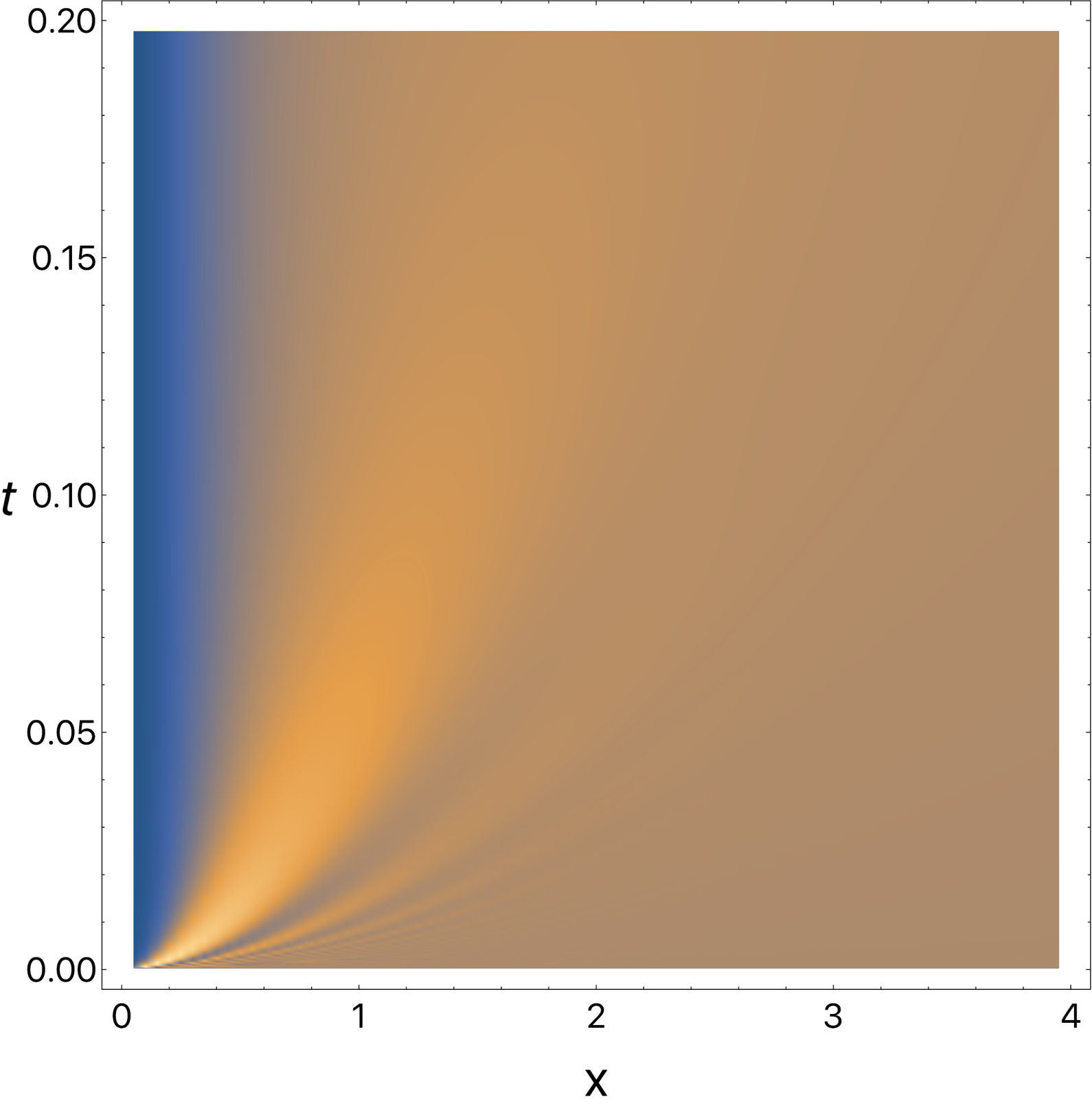
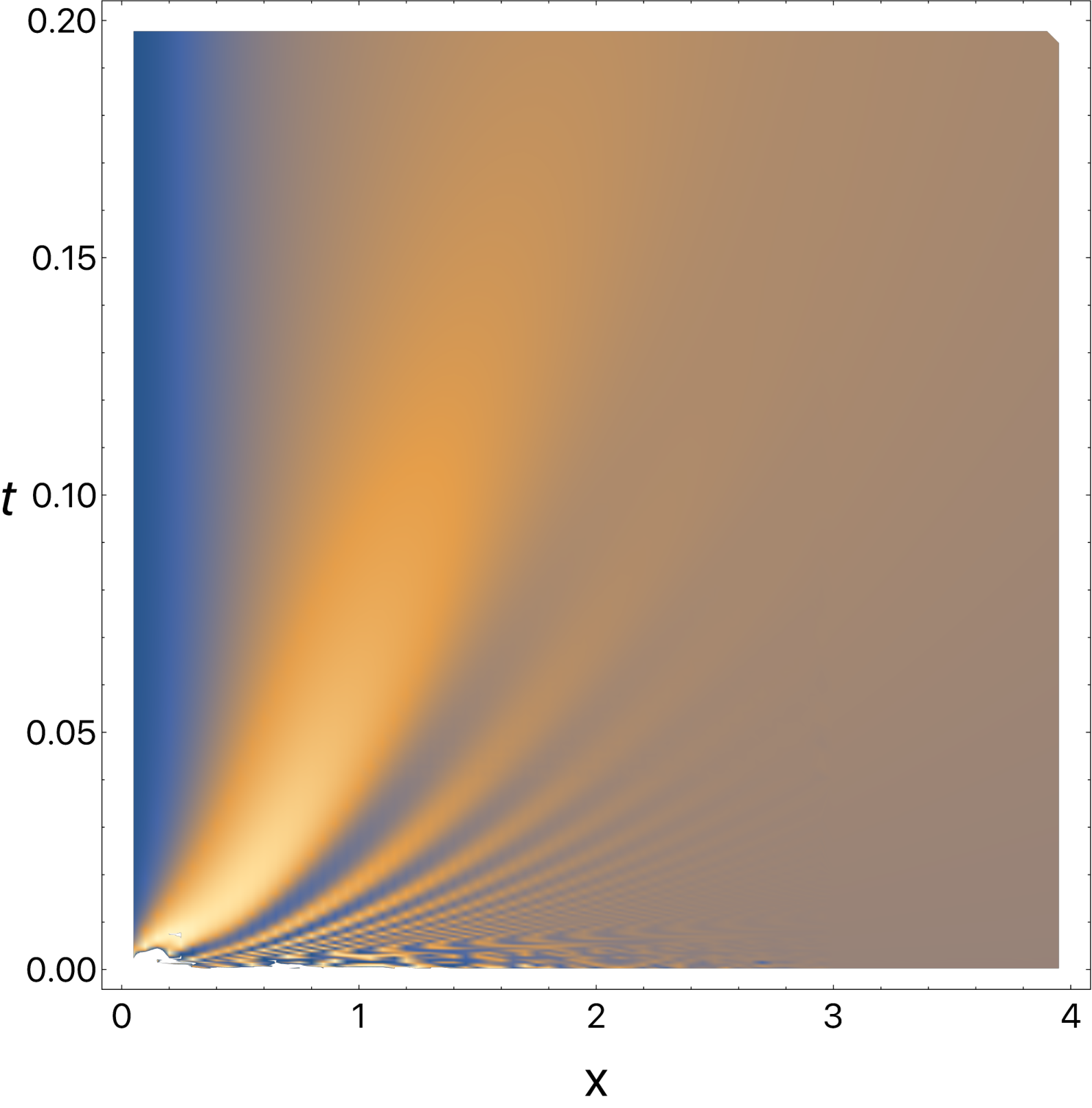
We see that for the chosen parameters $\mathcal{D}=1$ and $c=10$ the effects of the ${\cal O}(c^{-1})$ term are clearly visible and significantly modify the $c=\infty$ result. In particular the oscillatory behaviour as a function of distance for short times becomes more pronounced for smaller values of $c$. Perhaps the most striking feature of Fig. 3 is the apparent absence of any light cone effect [41]. This can be understood by noting that (i) our initial state has an infinite correlation length and any light cone like feature would therefore be weak; (ii) the local Hilbert space is infinite dimensional and the dispersion relation of elementary excitations unbounded. Hence the Lieb-Robinson bound [68] does not apply and “superluminal” effects [69] are allowed.

An alternative representation of (2.2) more suitable for numerical evaluations and an analysis of the $x\to 0$ and $t\to 0$ limits are presented in Appendix D.

The large $x$ and $t$ asymptotics of (2.2) at fixed ratio $\alpha=\frac{x}{4t}$ can be determined by a stationary phase approximation, which results in

$$\langle\sigma(x)\sigma(0)\rangle_{t}=(1+\tfrac{2\mathcal{D}}{c})^{2}\frac{\pi}{2|t|}\rho(\alpha^{\prime})\rho_{h}(\alpha^{\prime})+o(t^{-1})\,,$$

(26)

with $\alpha^{\prime}=\tfrac{x^{\prime}}{4t}$.

We discussed how to determine the non-equal time density-density correlation function in an arbitrary energy eigenstate described by a root density $\rho(\lambda)$ in our previous work [63]. The results in this Section are thus valid for a generic root density $\rho$, the steady state one (15) being a particular case. Applying the same method to the connected dynamical two-point function of $\sigma_{2}(x)$ gives the following result

	$\displaystyle\left\langle\sigma_{2}\left(x,\tau\right)\sigma_{2}\left(0,0\right)\right\rangle_{c}$	$\displaystyle=\underset{\epsilon\to 0}{\lim}\,\frac{16}{c^{4}}\int_{-\infty}^{\infty}\int_{-\infty}^{\infty}\rho(\lambda)\rho_{h}(\mu)\ G(\lambda,\mu)\ e^{i\tau(\lambda^{2}-\mu^{2})+ix(\mu-\lambda)-\epsilon\mu^{2}}\text{d}\lambda\text{d}\mu$
		$\displaystyle+\underset{\epsilon\to 0}{\lim}\,\frac{16}{c^{4}}\int_{-\infty}^{\infty}\int_{-\infty}^{\infty}\int_{-\infty}^{\infty}\int_{-\infty}^{\infty}\rho(\lambda)\rho_{h}(\mu)\rho(u)\rho_{h}(v)(\lambda-u)^{2}(\mu-v)^{2}$
		$\displaystyle\qquad\qquad\times e^{i\tau(\lambda^{2}-\mu^{2})+ix(\mu-\lambda)+i\tau(u^{2}-v^{2})+ix(v-u)-\epsilon\mu^{2}-\epsilon v^{2}}\text{d}\lambda\text{d}\mu\text{d}u\text{d}v$
		$\displaystyle+{\cal O}(c^{-5})\,,$		(27)

where we have defined

	$\displaystyle G(\lambda,\mu)$	$\displaystyle=\Big[\mathcal{E}+\mathcal{D}\lambda^{2}-2\lambda\mathcal{P}+(\mu-\lambda)(\mathcal{D}\lambda-\mathcal{P})\Big]^{2}\ ,$
	$\displaystyle\mathcal{P}$	$\displaystyle=\int_{-\infty}^{\infty}\lambda\rho(\lambda)\text{d}\lambda\,,\qquad\mathcal{E}=\int_{-\infty}^{\infty}\lambda^{2}\rho(\lambda)\text{d}\lambda\,.$		(28)

The result for the connected two-point function in the stationary state reached at late times after the quench is obtained by substituting the particle and hole densities (15) into (2.3) and (28). The leading asymptotic behaviour for large $x$ and $\tau$ with $\alpha=\frac{x}{2\tau}$ kept fixed can be obtained by a stationary phase approximation

$$\left\langle\sigma_{2}(x,\tau)\sigma_{2}(0,0)\right\rangle_{c}=\frac{16\pi}{c^{4}|\tau|}\rho(\alpha)\rho_{h}(\alpha)(\mathcal{D}\alpha^{2}-2{\cal P}\alpha+{\cal E})^{2}+{\cal O}(\tau^{-2})+{\cal O}(c^{-5})\,.$$

(29)

These results can be compared with predictions of Generalized Hydrodynamics [70]. According to these the leading large time and distance asymptotics of connected correlations between two local observables $\mathcal{O}_{1}$ and $\mathcal{O}_{2}$ is

$$\left\langle\mathcal{O}_{1}(x,\tau)\mathcal{O}_{2}(0,0)\right\rangle_{c}=\int_{-\infty}^{\infty}\delta(x-v^{\rm eff}(\lambda)\tau)\frac{\rho(\lambda)\rho_{h}(\lambda)}{\rho(\lambda)+\rho_{h}(\lambda)}V^{\mathcal{O}_{1}}(\lambda)V^{\mathcal{O}_{2}}(\lambda)\text{d}\lambda+o(\tau^{-1})\,,$$

(30)

where $V^{\mathcal{O}}(\lambda)$ is the so-called hydrodynamic projection of the operator $\mathcal{O}$, and $v^{\rm eff}(\lambda)$ the effective velocity associated with the macro-state defined by the particle and hole densities $\rho(\lambda)$ and $\rho_{h}(\lambda)$. The hydrodynamic projection $V^{\sigma_{2}}(\lambda)$ of $\sigma_{2}$ has been determined in [70]

$$V^{\sigma_{2}}(\lambda)=\frac{2}{\pi}\int_{-\infty}^{\infty}\frac{\rho(\mu)}{\rho(\mu)+\rho_{h}(\mu)}\frac{g_{\mu}^{\rm dr}(\lambda)}{h_{1}^{\rm dr}(\lambda)}(h_{2}^{\rm dr}(\mu)h_{1}^{\rm dr}(\lambda)-h_{1}^{\rm dr}(\mu)h_{2}^{\rm dr}(\lambda))\text{d}\mu\ .$$

(31)

Here $h_{n}(\lambda)=\lambda^{n-1}$, $g_{\mu}(\lambda)=\frac{\mu-\lambda}{(\lambda-\mu)^{2}+c^{2}}$, and the dressing operation $h^{\rm dr}$ is defined by

$$h^{\rm dr}(\lambda)=h(\lambda)+\frac{1}{2\pi}\int_{-\infty}^{\infty}\frac{2c}{c^{2}+(\lambda-\mu)^{2}}\frac{\rho(\mu)}{\rho(\mu)+\rho_{h}(\mu)}h^{\rm dr}(\mu)\text{d}\mu\,.$$

(32)

We find that the asymptotics (29) agrees with this GHD prediction at leading order in $1/c$.

The dynamical two-point function of $\sigma_{2}(x)$ is related to the Drude weight $D$ and the Onsager coefficient $\mathfrak{L}$ by

$$\frac{1}{2}\int_{-\infty}^{\infty}x^{2}\left[\left\langle\sigma_{2}(x,\tau)\sigma_{2}(0,0)\right\rangle+\left\langle\sigma_{2}(x,-\tau)\sigma_{2}(0,0)\right\rangle\right]\text{d}x=D\tau^{2}+\mathfrak{L}|\tau|+o(\tau)\ .$$

(33)

In contrast to the density-density correlator the two-point function of $\sigma_{2}(x)$ is expected to exhibit diffusive behaviour, i.e. have a non-vanishing Onsager coefficient $\mathfrak{L}\neq 0$. Our expression for the two point function translates into the following results for $D$ and $\mathfrak{L}$

	$\displaystyle D$	$\displaystyle=\frac{128\pi}{c^{4}}\int_{-\infty}^{\infty}\lambda^{2}\rho(\lambda)\rho_{h}(\lambda)[{\cal E}+{\cal D}\lambda^{2}-2\lambda{\cal P}]^{2}\text{d}\lambda+\mathcal{O}(c^{-5})\,,$
	$\displaystyle\mathfrak{L}$	$\displaystyle=\mathcal{O}(c^{-5})\,.$		(34)

This shows that higher orders in the $1/c$-expansion are required to determine the Onsager coefficient. We note that this specific result holds only for root densities $\rho$ that decay sufficiently fast at infinity. In the case of the steady state root density (15), because of the slow decay of the density, the next terms in the $1/c$ expansion should be re-summed to yield a convergent integral.

The time evolution of the expectation value of any operator $\mathcal{O}$ can always be expressed as a double sum over a basis of energy eigenstates

$$\langle\mathcal{O}\rangle_{t}=\sum_{\boldsymbol{\lambda},\boldsymbol{\mu}}\frac{\langle\Psi_{\rm BEC}|\boldsymbol{\lambda}\rangle\langle\boldsymbol{\lambda}|\mathcal{O}|\boldsymbol{\mu}\rangle\langle\boldsymbol{\mu}|\Psi_{\rm BEC}\rangle}{\langle\boldsymbol{\lambda}|\boldsymbol{\lambda}\rangle\langle\boldsymbol{\mu}|\boldsymbol{\mu}\rangle}e^{it(E(\boldsymbol{\lambda})-E(\boldsymbol{\mu}))}\,.$$

(35)

Here we have assumed that $\langle\Psi_{\rm BEC}|\Psi_{\rm BEC}\rangle=1$. The Quench Action approach [23] posits that one of the two sums in (35) is completely dominated by states around a saddle point characterized by a certain root distribution $\rho_{s}$ that is fixed by the overlaps. This allows one to rewrite (35) in the form

$$\lim_{L\to\infty}\langle\mathcal{O}\rangle_{t}=\lim_{L\to\infty}\frac{1}{|\mathfrak{S}_{L}|}\sum_{\boldsymbol{\lambda}\in\mathfrak{S}_{L}}{\rm Re}\bigg[\sum_{\boldsymbol{\mu}}\frac{\langle\Psi_{\rm BEC}|\boldsymbol{\mu}\rangle\langle\boldsymbol{\lambda}|\mathcal{O}|\boldsymbol{\mu}\rangle}{\langle\Psi_{\rm BEC}|\boldsymbol{\lambda}\rangle\langle\boldsymbol{\mu}|\boldsymbol{\mu}\rangle}e^{it(E(\boldsymbol{\lambda})-E(\boldsymbol{\mu}))}\bigg]\,,$$

(36)

i.e. a generalized micro-canonical average [23, 71] over a set $\mathfrak{S}_{L}$ of microstates corresponding to the root density $\rho_{s}$. Employing typicality ideas the micro-canonical average is then replaced by the expectation value with respect to a single “representative state” $|\boldsymbol{\lambda}\rangle$ [23]

$$\lim_{L\to\infty}\langle\mathcal{O}\rangle_{t}=\lim_{L\to\infty}{\rm Re}\bigg[\sum_{\boldsymbol{\mu}}\frac{\langle\Psi_{\rm BEC}|\boldsymbol{\mu}\rangle\langle\boldsymbol{\lambda}|\mathcal{O}|\boldsymbol{\mu}\rangle}{\langle\Psi_{\rm BEC}|\boldsymbol{\lambda}\rangle\langle\boldsymbol{\mu}|\boldsymbol{\mu}\rangle}e^{it(E(\boldsymbol{\lambda})-E(\boldsymbol{\mu}))}\bigg]\ .$$

(37)

We note that this last step implies that in the thermodynamic limit (37) depends on the representative state $|\boldsymbol{\lambda}\rangle$ only through its root density $\rho(\lambda)$.

To be of practical use the representation (37) requires closed-form expressions for the overlaps $\langle\Psi_{\rm BEC}|\boldsymbol{\lambda}\rangle$. For our quench protocol an efficient representation for the overlaps was derived in [28, 27]. Importantly, the overlaps are non-zero only for “pair” states, i.e. states whose rapidities are of the form $-\lambda_{N/2},...,-\lambda_{1},\lambda_{1},...,\lambda_{N/2}$ with $0<\lambda_{j}\ \forall j$. We will denote a set of positive $\lambda_{j}$ by $\boldsymbol{\lambda}>0$. We will use the notation $\boldsymbol{\bar{\lambda}}=(-\boldsymbol{\lambda})\cup\boldsymbol{\lambda}$ for such sets of rapidities. The overlaps are then given by

$$\frac{\langle\Psi_{\rm BEC}|\boldsymbol{\bar{\lambda}}\rangle}{\sqrt{\langle\boldsymbol{\bar{\lambda}}|\boldsymbol{\bar{\lambda}}\rangle}}=(-1)^{N/2}\sqrt{\frac{N!}{L^{N}}}\sqrt{\frac{\det G^{+}(\boldsymbol{\lambda})}{\det G^{-}(\boldsymbol{\lambda})}}\frac{1}{\prod_{j=1}^{N/2}\lambda_{j}\sqrt{\frac{\lambda_{j}^{2}}{c^{2}}+\frac{1}{4}}}\,,$$

(38)

where $G^{\pm}(\boldsymbol{\lambda})$ are $(N/2)\times(N/2)$ matrices of the form

	$\displaystyle G^{\pm}_{ij}(\boldsymbol{\lambda})=$	$\displaystyle\delta_{ij}\bigg(1+\frac{1}{L}\sum_{k=1}^{N/2}\frac{2c}{c^{2}+(\lambda_{i}-\lambda_{k})^{2}}+\frac{2c}{c^{2}+(\lambda_{i}+\lambda_{k})^{2}}\bigg)$
		$\displaystyle-\left(\frac{1}{L}\frac{2c}{c^{2}+(\lambda_{i}-\lambda_{j})^{2}}\pm\frac{1}{L}\frac{2c}{c^{2}+(\lambda_{i}+\lambda_{j})^{2}}\right)\,.$		(39)

For our quench protocol the saddle point root distribution was determined in Ref. [28] and is given in (15).

Our objective is to combine the Quench Action approach to non-equilibrium dynamics (36) with a strong coupling expansion around $c=\infty$. A detailed exposition of the $1/c$ expansion technique for dynamical correlation functions in equilibrium has been given in [63]. In the following we recall the key steps of the method and then extend it to the out-of-equilibrium case.

In order to facilitate the $1/c$-expansion of the form factors and Bethe equations we first fix an arbitrary, large $\Lambda>0$ that will be sent to $\infty$ at the end of the calculation. We then select an arbitrary averaging state $\boldsymbol{\lambda}$ by fixing its Bethe numbers $\boldsymbol{I}$, impose the constraint that $\forall i,\,|\lambda_{i}|<\Lambda$, and define the following overlap-weighted spectral sum

$$\langle\mathcal{O}\rangle^{[\boldsymbol{\lambda}],\Lambda}_{t}\equiv{\rm Re}\bigg[\sum_{\begin{subarray}{c}\boldsymbol{\mu}\\ \forall i,\,|\mu_{i}|<\Lambda\end{subarray}}\frac{\langle\Psi_{\rm BEC}|\boldsymbol{\mu}\rangle\langle\boldsymbol{\lambda}|\mathcal{O}|\boldsymbol{\mu}\rangle}{\langle\Psi_{\rm BEC}|\boldsymbol{\lambda}\rangle\langle\boldsymbol{\mu}|\boldsymbol{\mu}\rangle}e^{it(E(\boldsymbol{\lambda})-E(\boldsymbol{\mu}))}\bigg]\,.$$

(40)

The overlap-weighted form factor can then be expanded in powers of $1/c$ at fixed $L,\boldsymbol{I}$

$$\frac{\langle\Psi_{\rm BEC}|\boldsymbol{\mu}\rangle\langle\boldsymbol{\lambda}|\mathcal{O}|\boldsymbol{\mu}\rangle}{\langle\Psi_{\rm BEC}|\boldsymbol{\lambda}\rangle\langle\boldsymbol{\mu}|\boldsymbol{\mu}\rangle}=\sum_{n=0}^{\infty}\frac{F_{n}(\boldsymbol{I},\boldsymbol{J})}{c^{n}}\,,$$

(41)

where $\boldsymbol{J}$ denotes the Bethe numbers of $\boldsymbol{\mu}$. We also expand the argument of the phase

$$E(\boldsymbol{\lambda})-E(\boldsymbol{\mu})=\sum_{n=0}^{\infty}\frac{E_{n}(\boldsymbol{I})-E_{n}(\boldsymbol{J})}{c^{n}}\,,$$

(42)

but do not expand the phase $e^{it(E(\boldsymbol{\lambda})-E(\boldsymbol{\mu}))}$ itself in powers of $1/c$. The truncation of the resulting series at a given order $\mathcal{O}(c^{-m})$ defines the $m$-th term of our expansion. Once this truncation has been done, the thermodynamic limit and (if necessary) the average in (36) can be performed. By construction, the result depends only on the root density $\rho$ of the fixed averaging state $\boldsymbol{\lambda}$.

Finally one would like to take the limit $\Lambda\to\infty$. As we will see, the thermodynamic limit of the quantity $\langle\mathcal{O}\rangle^{[\boldsymbol{\lambda}],\Lambda}_{t}$ at finite $\Lambda>0$ involves integrals of the form

$$I_{n}(\Lambda|t,x)=\int_{-\Lambda}^{\Lambda}\mu^{n}e^{-it\mu^{2}+ix\mu}\text{d}\mu\ .$$

(43)

The limit $\Lambda\to\infty$ of these integrals for $n>0$ only exists in a distribution sense, i.e. their integral with any smooth function of $x,t$ has a well-defined limit when $\Lambda\to\infty$. The resulting limits are denoted by $I_{n}(t,x)$ and have been worked out in [63] for $n=0,1,2$

	$\displaystyle I_{1}(t,x)$	$\displaystyle=\frac{x}{2t}I_{0}(x,t)\ ,$
	$\displaystyle I_{2}(t,x)$	$\displaystyle=\left(\left(\frac{x}{2t}\right)^{2}+\frac{1}{2it}\right)I_{0}(x,t)\ ,$
	$\displaystyle I_{0}(t,x)$	$\displaystyle=\int_{-\infty}^{\infty}e^{-it\mu^{2}+ix\mu}\text{d}\mu\,.$		(44)

An equivalent representation is

$$I_{n}(t,x)=\lim_{\epsilon\to 0}\,\int_{-\infty}^{\infty}\mu^{n}e^{-it\mu^{2}+ix\mu-\epsilon\mu^{2}}\text{d}\mu\,.$$

(45)

The process described above provides closed-form expressions at order $\mathcal{O}(c^{-m})$ for the quantities

$$\langle\mathcal{O}\rangle^{[\rho]}_{t}\equiv\lim_{\Lambda\to\infty}\lim_{L\to\infty}\frac{1}{|\mathfrak{S}_{L}|}\sum_{\boldsymbol{\lambda}\in\mathfrak{S}_{L}}\langle\mathcal{O}\rangle^{[\boldsymbol{\lambda}],\Lambda}_{t}\,.$$

(46)

Finally, in order to obtain the out-of-equilibrium time evolution (36) this result needs to be evaluated for the saddle point root density $\rho$ describing the quench protocol of interest.

In order to evaluate the expression (36), one requires a closed-form expression for the form factors of $\sigma_{2}$ between energy eigenstates. In the case of interest, because of the structure of the non-vanishing overlaps with the initial state $|\Psi_{\rm BEC}\rangle$, the states entering (36) have a pair structure and will be denoteed $|\boldsymbol{\bar{\lambda}}\rangle$ and $|\boldsymbol{\bar{\mu}}\rangle$. Hence they have same (vanishing) momentum. In this situation the normalized form factors have been calculated previously and read[78]

	$\displaystyle\frac{\left\langle\boldsymbol{\mu}|\sigma_{2}\left(0\right)|\boldsymbol{\lambda}\right\rangle}{\sqrt{\left\langle\boldsymbol{\lambda}\left|\boldsymbol{\lambda}\right\rangle\left\langle\boldsymbol{\mu}\right|\boldsymbol{\mu}\right\rangle}}$	$\displaystyle=\frac{(-i)^{N+1}(-1)^{N(N-1)/2}}{2cL^{N}\sqrt{\det G(\boldsymbol{\lambda})\det G(\boldsymbol{\mu})}}\frac{(E(\boldsymbol{\mu})-E(\boldsymbol{\lambda}))^{2}}{N}\prod_{j\neq p}(V_{j}^{+}-V_{j}^{-})$
		$\displaystyle\times\frac{\prod_{i<j}|\lambda_{i}-\lambda_{j}|\prod_{i<j}|\mu_{i}-\mu_{j}|}{\prod_{i,j}(\lambda_{i}-\mu_{j})}\sqrt{\prod_{i,j}\frac{\lambda_{i}-\lambda_{j}+ic}{\mu_{i}-\mu_{j}+ic}}\,\,\underset{i,j=1,...,N}{\det}\Bigg[\delta_{ij}+U_{ij}\Bigg].$		(47)

Here $1\leq p\leq N$ is an arbitrary integer and

References

- [1] A. Polkovnikov, K. Sengupta, A. Silva and M. Vengalattore, Colloquium: Nonequilibrium dynamics of closed interacting quantum systems, Rev. Mod. Phys. 83, 863 (2011).
- [2] F. H. L. Essler and M. Fagotti, Quench dynamics and relaxation in isolated integrable quantum spin chains, J. Stat. Mech. 064002 (2016).
- [3] L. D’Alessio, Y. Kafri, A. Polkovnikov and M. Rigol, From quantum chaos and eigenstate thermalization to statistical mechanics and thermodynamics, Adv. Phys. 65(3), 239 (2016).
- [4] C. Gogolin and J. Eisert, Equilibration, thermalisation, and the emergence of statistical mechanics in closed quantum systems, Rep. Prog. Phys. 79(5), 056001 (2016).
- [5] P. Calabrese and J. Cardy, Quantum quenches in dimensional conformal field theories, J. Stat. Mech. 064003 (2016).
- [6] T. Langen, T. Gasenzer and J. Schmiedmayer, Prethermalization and universal dynamics in near-integrable quantum systems, J. Stat. Mech. 064009,(2016).
- [7] M. Greiner, O. Mandel, T.W. Hänsch, and I. Bloch, Collapse and revival of the matter wave field of a Bose-Einstein condensate, Nature 419, 51-54 (2002).
- [8] T. Kinoshita, T. Wenger, D. S. Weiss, A quantum Newton’s cradle, Nature 440, 900 (2006).
- [9] S. Hofferberth, I. Lesanovsky, B. Fischer, T. Schumm, and J. Schmiedmayer, Non-equilibrium coherence dynamics in one-dimensional Bose gases, Nature 449, 324-327 (2007).
- [10] S. Trotzky Y.-A. Chen, A. Flesch, I. P. McCulloch, U. Schollwöck, J. Eisert, and I. Bloch, Probing the relaxation towards equilibrium in an isolated strongly correlated 1D Bose gas, Nature Phys. 8, 325 (2012).
- [11] M. Gring, M. Kuhnert, T. Langen, T. Kitagawa, B. Rauer, M. Schreitl, I. Mazets, D. A. Smith, E. Demler, and J. Schmiedmayer, Relaxation Dynamics and Pre-thermalization in an Isolated Quantum System, Science 337, 1318 (2012).
- [12] U. Schneider, L. Hackermüller, J. P. Ronzheimer, S. Will, S. Braun, T. Best, I. Bloch, E. Demler, S. Mandt, D. Rasch, and A. Rosch, Fermionic transport and out-of-equilibrium dynamics in a homogeneous Hubbard model with ultracold atoms, Nature Phys. 8, 213 (2012).
- [13] M. Cheneau, P. Barmettler, D. Poletti, M. Endres, P. Schauss, T. Fukuhara, C. Gross, I. Bloch, C. Kollath, and S. Kuhr, Light-cone-like spreading of correlations in a quantum many-body system, Nature 481, 484 (2012).
- [14] F. Meinert, M.J. Mark, E. Kirilov, K. Lauber, P. Weinmann, A.J. Daley, and H.-C. Nägerl, Quantum Quench in an Atomic One-Dimensional Ising Chain, Phys. Rev. Lett. 111, 053003 (2013).
- [15] T. Fukuhara, A. Kantian, M. Endres, M. Cheneau, P. Schauß, S. Hild, D. Bellem, U. Schollwöck, T. Giamarchi, C. Gross, I. Bloch, and S. Kuhr, Quantum dynamics of a mobile spin impurity, Nature Physics 9, 235 (2013).
- [16] N. Navon, A.L. Gaunt, R.P. Smith and Z. Hadzibabic, Critical Dynamics of Spontaneous Symmetry Breaking in a Homogeneous Bose gas, Science 347, 167 (2015).
- [17] M. Schemmer, I. Bouchoule, B. Doyon and J. Dubail, Generalized HydroDynamics on an Atom Chip, Phys. Rev. Lett. 122, 090601 (2019).
- [18] M. Rigol, V. Dunjko, V. Yurovsky, and M. Olshanii, Relaxation in a Completely Integrable Many-Body Quantum System: An Ab Initio Study of the Dynamics of the Highly Excited States of 1D Lattice Hard-Core Bosons, Phys. Rev. Lett. 98, 50405 (2007).
- [19] P. Calabrese, F.H.L. Essler, and M. Fagotti, Quantum Quench in the Transverse-Field Ising Chain, Phys. Rev. Lett. 106, 227203 (2011).
- [20] P. Calabrese, F.H.L. Essler, and M. Fagotti, Quantum Quench in the Transverse Field Ising Chain II: Stationary State Properties, J. Stat. Mech. (2012) P07022.
- [21] B. Pozsgay, The generalized Gibbs ensemble for Heisenberg spin chains, J. Stat. Mech. (2013) P07003.
- [22] M. Fagotti and F.H.L. Essler, Stationary behaviour of observables after a quantum quench in the spin-1/2 Heisenberg XXZ chain, J. Stat. Mech. (2013) P07012.
- [23] J.-S. Caux and F.H.L. Essler, Time Evolution of Local Observables After Quenching to an Integrable Model, Phys. Rev. Lett. 110, 257203 (2013).
- [24] M. Kormos, A. Shashi, Y.-Z. Chou, J.-S. Caux and A. Imambekov, Interaction quenches in the one-dimensional Bose gas, Phys. Rev. B 88, 205131 (2013).
- [25] M, Fagotti, M, Collura, F.H.L. Essler, and P. Calabrese, Relaxation after quantum quenches in the spin-1/2 Heisenberg XXZ chain, Phys. Rev. B 89, 125101 (2014).
- [26] B. Wouters, J. De Nardis, M. Brockmann, D. Fioretto, M. Rigol, and J.-S. Caux, Quenching the Anisotropic Heisenberg Chain: Exact Solution and Generalized Gibbs Ensemble Predictions, Phys. Rev. Lett. 113, 117202 (2014).
- [27] M. Brockmann, B. Wouters, D. Fioretto, J. De Nardis, R. Vlijm and J.-S. Caux, Quench action approach for releasing the Néel state into the spin-1/2 XXZ chain, Stat. Mech. (2014) P12009.
- [28] J. De Nardis, B. Wouters, M. Brockmann, and J.-S. Caux, Solution for an interaction quench in the Lieb-Liniger Bose gas, Phys. Rev. A 89, 033601 (2014).
- [29] B. Pozsgay, M. Mestyán, M.A. Werner, M. Kormos, G. Zaránd, and G. Takács, Correlations after Quantum Quenches in the XXZ Spin Chain: Failure of the Generalized Gibbs Ensemble, Phys. Rev. Lett. 113, 117203 (2014).
- [30] B. Pozsgay, Quantum quenches and generalized Gibbs ensemble in a Bethe Ansatz solvable lattice model of interacting bosons, J. Stat. Mech. (2014) P10045.
- [31] G. Goldstein and N. Andrei, Failure of the GGE hypothesis for integrable models with bound states, Phys. Rev. A90, 043625 (2014).
- [32] M. Mestyán, B. Pozsgay, G. Takács, and M.A. Werner, Quenching the XXZ spin chain: quench action approach versus generalized Gibbs ensemble, J. Stat. Mech. (2015) P04001.
- [33] E. Ilievski, M. Medenjak, T. Prosen and L. Zadnik, Quasilocal charges in integrable lattice systems, J. Stat. Mech. 064008, (2016).
- [34] E. Ilievski, J. De Nardis, B. Wouters, J.-S. Caux, F.H.L. Essler, T. Prosen, Complete Generalized Gibbs Ensemble in an interacting Theory, Phys. Rev. Lett. 115, 157201 (2015).
- [35] E. Ilievski, E. Quinn, J. De Nardis and M. Brockmann, String-charge duality in integrable lattice models, J. Stat. Mech. 063101 (2016).
- [36] L. Piroli, P. Calabrese, and F.H.L. Essler, Multiparticle Bound-State Formation following a Quantum Quench to the One-Dimensional Bose Gas with Attractive Interactions, Phys. Rev. Lett. 116, 070408 (2016).
- [37] L. Piroli, P. Calabrese, and F.H.L. Essler, Quantum quenches to the attractive one-dimensional Bose gas: exact results SciPost Phys. 1, 001 (2016).
- [38] S. Sotiriadis, Memory-preserving equilibration after a quantum quench in a 1d critical model, Phys. Rev. A 94, 031605 (2016).
- [39] J. Cardy, Quantum quenches to a critical point in one dimension: some further results, J. Stat. Mech. (2016) 023103.
- [40] P. Calabrese and J. Cardy, Time Dependence of Correlation Functions Following a Quantum Quench, Phys. Rev. Lett. 96, 136801 (2006).
- [41] P. Calabrese and J. Cardy, Quantum quenches in extended systems, J. Stat. Mech. (2007) P06008.
- [42] P. Calabrese, F.H.L. Essler, and M. Fagotti, Quantum quench in the transverse field Ising chain: I. Time evolution of order parameter correlators. J. Stat. Mech. (2012) P07016.
- [43] J. De Nardis and J.-S. Caux, Analytical expression for a post-quench time evolution of the one-body density matrix of one-dimensional hard-core bosons, J. Stat. Mech. (2014) P12012.
- [44] M. Kormos, M. Collura and P. Calabrese, Analytic results for a quantum quench from free to hard-core one-dimensional bosons, Phys. Rev. A 89, 013609 (2014).
- [45] D. Schuricht and F.H.L. Essler, Dynamics in the Ising field theory after a quantum quench, J. Stat. Mech. P04017 (2012).
- [46] B. Bertini, D. Schuricht, and F.H.L. Essler, Quantum quench in the sine-Gordon model, J. Stat. Mech. (2014) P10035.
- [47] A. Cortés Cubero and D. Schuricht, Quantum quench in the attractive regime of the sine-Gordon model, J. Stat. Mech. 103106 (2017).
- [48] D. X. Horvath, M. Kormos and G. Takacs, Overlap singularity and time evolution in integrable quantum field theory, JHEP 08 170 (2018).
- [49] H. Rieger and F. Iglói, Semiclassical theory for quantum quenches in finite transverse Ising chains, Phys. Rev. B 84, 165117 (2011).
- [50] S. Evangelisti, Semi-classical theory for quantum quenches in the O(3) non-linear sigma model, J. Stat. Mech. (2013) P04003.
- [51] M. Kormos and G. Zaránd, Quantum quenches in the sine-Gordon model: a semiclassical approach, Phys. Rev. E 93, 062101 (2016).
- [52] J.-S. Caux, The Quench Action, J. Stat. Mech. , 064006 (2016).
- [53] J. De Nardis, L. Piroli and J.-S. Caux, Relaxation dynamics of local observables in integrable systems, Phys. A: Math. Theor. 48 43FT01 (2015).
- [54] E. Granet, M. Fagotti and F.H.L. Essler, Finite temperature and quench dynamics in the Transverse Field Ising Model from form factor expansions, SciPost Phys. 9, 033 (2020).
- [55] M. Brockmann, J. De Nardis, B. Wouters, and J.-S. Caux, A Gaudin-like determinant for overlaps of Néel and XXZ Bethe states, J. Phys. A47, 145003 (2014).
- [56] B. Pozsgay, Overlaps between eigenstates of the XXZ spin-1/2 chain and a class of simple product states, J. Stat. Mech. , P06011 (2014).
- [57] L. Piroli, B. Pozsgay, and E. Vernier, What is an integrable quench?, Nucl. Phys. B 925, 362 (2017).
- [58] M. de Leeuw, C. Kristjansen, and S. Mori, AdS/dCFT one-point functions of the SU(3) sector, Phys. Lett. B 763, 197 (2016).
- [59] M. Mestyan, B. Bertini, L. Piroli and P. Calabrese Exact solution for the quench dynamics of a nested integrable system, J. Stat. Mech. (2017).
- [60] B. Pozsgay, Overlaps with arbitrary two-site states in the XXZ spin chain, J. Stat. Mech. 053103 (2018).
- [61] B. Pozsgay, L. Piroli, and E. Vernier, “Integrable Matrix Product States from boundary integrability,” SciPost Phys. 6, 062 (2019).
- [62] Y. Jiang and B. Pozsgay, On exact overlaps in integrable spin chains, JHEP 22 (2020).
- [63] E. Granet and F. H. L. Essler, A systematic -expansion of form factor sums for dynamical correlations in the Lieb-Liniger model, SciPost Phys. 9, 082 (2020).
- [64] E. H. Lieb and W. Liniger, Exact Analysis of an Interacting Bose Gas. I. The General Solution and the Ground State, Phys. Rev. 130, 1605 (1963).
- [65] F.A. Brézin, G.P. Pohil and V.M. Finkelberg, The Schrödinger equation for a system of one-dimensional particles with point interactions., Viest. Mosk. Uni. 1, 21-28 (1964).
- [66] V. E. Korepin, N. M. Bogoliubov and A. G. Izergin, Quantum inverse scattering method and correlation functions, Cambridge University Press (1993).
- [67] G. Lang, Conjectures about the structure of strong- and weak-coupling expansions of a few ground-state observables in the Lieb-Liniger and Yang-Gaudin models, SciPost Phys. 7, 055 (2019).
- [68] E. H. Lieb and D. W. Robinson, The finite group velocity of quantum spin systems, Commun. Math. Phys. 28, 251 (1972).
- [69] B. Bertini, Approximate light cone effects in a non-relativistic quantum field theory after a local quench, Phys. Rev. B 95, 075153 (2017).
- [70] B. Doyon, Exact large-scale correlations in integrable systems out of equilibrium, SciPost Phys. 5, 054 (2018).
- [71] A. C. Cassidy, C. W. Clark, and M. Rigol, Generalized Thermalization in an Integrable Lattice System, Phys. Rev. Lett. 106, 140405 (2011).
- [72] V. E. Korepin, Calculation of norms of Bethe wave functions, Comm. Math. Phys. 86, 391 (1982).
- [73] N.A. Slavnov, Calculation of scalar products of wave functions and form factors in the framework of the algebraic Bethe ansatz, Theor. Math. Phys. 79, 502 (1989).
- [74] N.A. Slavnov, Nonequal-time current correlation function in a one-dimensional Bose gas, Theor. Math. Phys. 82, 273 (1990).
- [75] V.E. Korepin and N.A. Slavnov, The form factors in the finite volume., Int. J. Mod. Phys. B 13, 2933 (1999).
- [76] T. Oota, Quantum projectors and local operators in lattice integrable models., J. Phys. A: Math. Gen. 37, 441 (2004).
- [77] K.K. Kozlowski, On form factors of the conjugated field in the non-linear Schrödinger model., J. Math. Phys. 52, 083302 (2011).
- [78] L. Piroli and P. Calabrese, Exact formulas for the form factors of local operators in the Lieb-Liniger model, J. Phys. A: Math. Theor. 48, 454002 (2015).
- [79] A.J.A. James, W.D. Goetze and F.H.L. Essler, Finite Temperature Dynamical Structure Factor of the Heisenberg-Ising Chain, Phys. Rev. B 79, 214408 (2009).
- [80] M. Collura and F.H.L. Essler, How order melts after quantum quenches, Phys. Rev. B 101, 041110(R) (2020).
- [81] L. Zadnik and M. Fagotti, The Folded Spin-1/2 XXZ Model: I. Diagonalisation, Jamming, and Ground State Properties, arXiv:2009.04995.
- [82] L. Zadnik, K. Bidzhiev and M. Fagotti, The Folded Spin-1/2 XXZ Model: II. Thermodynamics and Hydrodynamics with a Minimal Set of Charges, arXiv:2011.01159.
- [83] A. de Luca, G. Martelloni and J. Viti, Stationary states in a free fermionic chain from the quench action method, Phys. Rev. A 91, 021603 (2015).
- [84] A. Cortés Cubero, How generalized hydrodynamics time evolution arises from a form factor expansion, arXiv:2001.03065.