跳到论文正文
W Papers独立论文阅读器 arXiv:2102.09776 论文正文 计算阅读时间 · 0%
引用这篇论文根据当前论文元数据生成,正式投稿前建议核对。


License: CC BY 4.0
arXiv:2102.09776v1 [gr-qc] 19 Feb 2021

Generating spiky solutions of Einstein field equations with the Stephani transformation

Muhammad Zubair Ali Moughal
Abstract

The Geroch/Stephani transformation is a solution-generating transformation, and may generate spiky solutions. The spikes in solutions generated so far are either early-time permanent spikes or transient spikes. We want to generate a solution with a late-time permanent spike. We achieve this by applying the Stephani transformation with the rotational Killing vector field of the locally rotationally symmetric Jacobs solution. The late-time permanent spike occurs along the cylindrical axis. The generated solution also features a rich variety of transient structures. We introduce a new technique to analyse these structures. Our findings lead us to discover a transient behaviour, which we call the overshoot transition.

Acknowledgements.
In the name of Allah, The Most Gracious and The Most Merciful, who provided me the opportunity to unveil the concealed realities in the world of Mathematics. In the first place, I owe my deepest gratitude to my supervisor, Dr. Woei Chet Lim. It would have been next to impossible to write this dissertation without the guidance and valuable input/feedback of my respected supervisor. He is a source of true inspiration as he has always supported and guided me during my stay in New Zealand – especially his financial and personal support for providing a grant to present my work at the 22nd International Conference on General Relativity and Gravitation (GR22) and the 10th Australasian Conference on General Relativity and Gravitation (ACGRG10). I deeply acknowledge the role of the Department of Mathematics at University of Waikato which facilitated and provided learning and a healthy environment to complete my thesis. I am also thankful to the other PhD lab students Ejaz, Liam, Fahim, Hamish, Chris and Nick for a healthy working environment. My acknowledgment will never be complete without the special mention of my friends: Bilal, Hassam, Humair, Irfan, Atta, Irfan Habib, Shaheer, Mairaj and many more (it is not feasible to name all here). Thanks for being around and sharing several good times together during my stay in the University and New Zealand. I owe a special debt to my affectionate and lovely parents. The credit, for my enjoying this status in my life, goes to my parents. I donot have words to convey my cordial regards and thanks to my mother for her utmost efforts, sacrifices, and prayers. I am also grateful to my father for all that he did for my bright future. Besides I cannot dare to forget to mention the co-operation of my sweet sister, brothers and their naughty kids. I appreciate the moral support of my friends in Pakistan as well, specially Khalil, Kamran, Hassan, Faraz and Waqas. Lastly, I would like to thank the Higher Education Commission (H.E.C) of the government of Pakistan that provided me with the scholarship to do this PhD.

Chapter 0 Introduction

1 What is spike

The big bang theory postulates that the universe has always been expand- ing. Extrapolating this into the past, there was a time when the universe was incredibly dense and hot, such that even the laws of Einstein’s general relativity, which predicted the big bang, fail. Such time or place is called a singularity. Similarly, after depleting their nuclear fuel, massive stars can collapse under their own weight and become black holes. Inside a black hole, the collapse also inevitably leads to an incredibly dense and hot state where the laws of general relativity fail again. In the final stage before the laws fail, spacetime undergoes a kind of chaotic dynamics called Mixmaster or BKL dy- namics  [1, 2, 3, 4]. Under the influence of Mixmaster dynamics, a collapsing object is crushed or stretched at predictable and alternating speeds along its three dimensions. But what is really being crushed and stretched is space itself, regardless of the presence of any object there. Spikes form when adjacent parts of space experience vastly different rates of crushing and stretching. It is important to understand spikes because it occurs during a regime that transitions into the quantum regime, and quantum gravity researchers need to understand what happens during the transition. In another context, spike can also help explain the formation of large scale structure at late times.

On approach to the singularity a generic solution is approximated by a sequence of Kasner states, described by the Kasner solution of Einstein field equations (EFEs). The transition between Kasner states is approximated by another exact solution, the Taub solution. Furthermore, this transition can be achieved in two ways, as reflected by the sign of a curvature variable. In a spatially inhomogeneous model, this curvature variable may change sign from one place to another. As a result, transition fails to occur in a normal way at places where this curvature variable is zero. A different, inhomogeneous, dynamics occur instead, and this is the spike [5].

What is the mechanism behind spike formation? Briefly, when a solution is close to an unstable background solution that is represented by a saddle point in the state space, it generally becomes unstable. If the initial condition is such that the solution straddles the separatrix of the saddle point, then as the solution becomes unstable, some region of spacetime evolves one way, the other region evolves in a different way. The boundary between these two parts evolves in a way that is different from both regions (because on this boundary, its state lies exactly on the separatrix), and this creates a spiky inhomogeneity in the neighborhood of this boundary [5, 6].

2 The journey from numerical to exact solution

It is a general feature of solutions of partial differential equations that spikes occur  [7]. As Einstein field equations (EFEs) of general relativity are a set of partial differential equations, spikes can arise in the solutions of these equations  [5]. Spikes were first discovered in numerical simulations by Berger and Moncrief in 1993  [8]. In their numerical study on the so-called T3T^{3} Gowdy model11 1 T3T^{3} Gowdy models are orthogonally transitive G2G_{2} models with toroidal spatial topology. See Appendix B. [9], where the BKL dynamics terminates at a final Kasner state, they observed the development of large spatial derivatives near the singularity, which they termed as spiky features. These spikes are permanent spikes as their amplitude does not tend to zero towards singularity [10]. Furthermore, based on the work by Grubisˇ\check{\text{s}}ic´\acute{\text{c}} and Moncrief of the same year [11], these structures where found to occur in the neighbourhood of isolated spatial surfaces. Toward the end of the 1990s, Berger, Moncrief and co-workers had found further numerical evidence that the BKL picture seemed to be correct generically but there were difficulties in simulating these spikes  [12, 13, 14, 15]. Also, Hern in his PhD thesis [16] resolved individual spatially spiky features to high numerical accuracy but for a short time interval. The observed inhomogeneity of the curvature invariants makes it clear that the spikes are physical features of the spacetime not effects of the coordinate system.

In 2001 Rendall and Weaver [17] made a significant analytic step toward the understanding of spikes. They discovered a composition of two transformations that can map a spike-free solution to a solution with spike. They applied the solution-generating transformation and Fuchsian methods22 2 The theory of Fuchsian equations has been applied to analyse singularities in a variety of classes of spacetimes in general relativity. In [18, 19], Fuchsian algorithm is applied to Einstein’s equations to establish the existence of a family of solutions. Recent work can be found in [20], [21]. in [18, 22], to produce asymptotic expansions for spikes. In their numerical study they find false and true(real) spikes. False spikes are an effect of parameterisation of the metric, not a geometrical one, while true spikes are the geometric change, which they check by observing highly non-uniform behaviour in curvature invariants. The work on spiky features in Gowdy spacetimes by Rendall and Weaver was followed up by Garfinkle and Weaver in 2003, who used two different complementary numerical techniques [23]. In particular they studied the so-called (transient and recurring) high-velocity spikes and found that they eventually evolve into permanent low-velocity spikes. Also, Lim in his PhD thesis [5] applied the Rendall-Weaver transformation on the Wainwright-Marshman solution [24]. He obtained a new explicit vacuum OT G2G_{2} (Appendix B) solution that develops a permanent spike.

After the 1993 discovery of spikes many researchers tried to understand the behaviour and dynamics of these structure. They put a lot of effort to solve it through numerical solutions and analytical approximation. In the beginning these analytical approximation were insufficient and the numerical simulations lack resolution. In 2008 [25], Lim discovered the first exact spike solution. Iteratively, he applied the Rendall-Weaver transformation on Kasner seed solution. The generated spike solution admits two Killing vector fields (KVFs) and it is an orthogonally transitive (OT) G2G_{2} solution (see Appendix B). This exact solution is the gateway to the understanding and analysis of the spikes. There was a question whether numerical solutions match the exact solution. The answer is yes – in 2009 Lim e​tet a​l.al. [26] using a new zooming technique, provided highly accurate numerical evidence.

Nungesser and Lim [27] found the inhomogeneous electromagnetic spike solution. They use the existing relation between vacuum Gowdy spacetime and electromagnetic Gowdy spacetime to find this new explicit solution. Beyer and Hennig [28] derived a family of Gowdy-symmetric generalized Taub–NUT solutions and found both false and true spikes.

Coley and Lim [29] discussed the influence of spikes on matter that leads to the formation of large scale structure at the early universe. They concentrated on how spikes generate matter overdensities in a radiation fluid in a special class of inhomogeneous models. In 2014 Lim and Coley [30] examined the tilted fluid, whose tilt provided another mechanism in generating matter inhomogeneity through the divergence term.

Coley and Lim [6] demonstrated the spike phenomenon by using the Lemaître-Tolman-Bondi (LTB) model. The LTB model is an exact solution that makes it easier to construct the spike. In this paper, they showed that spikes do not form in the matter density directly, it forms in the curvature as in [29]. They also explained that spike can provide an alternate contribution to the formation of large scale structures in the Universe.

The OT G2G_{2} spike solution contains permanent spikes, and there is a debate whether in the non-OT G2G_{2} solution these permanent spikes are unresolved spike transitions or are really permanent. In other words, would the yet undiscovered non-OT G2G_{2} spike solution contain permanent spikes? Numerical evidence suggests that the permanent spikes are unresolved spike transitions. Heinzle e​tet a​l.al. [31] described how BKL and spike oscillations arise from concatenations of exact solutions, suggesting the existence of hidden symmetries and showing that the results of BKL are part of a greater picture. Woei Chet Lim used Geroch’s transformation33 3 In 1971-72, Geroch wrote two papers on generating new exact solutions of Einsteins field equations by using a transformation [32, 33]. The transformation acts on a vacuum solution of Einstein field equations that possesses at least one KVF. This KVF remains preserved in the transformed solution. The stiff fluid version of Geroch transformation was given by Stephani in 1988 [34]. to discover the non-OT G2G_{2} spike solution in 2015. He applied the transformation to a Kasner seed solution, with a generic linear combination of KVFs [35]. He showed that non-OT G2G_{2} spike solution always resolves its spike as opposed to previous OT G2G_{2} solutions. This method shows a new way to generate various kinds of spikes.

The above advancements were made in the particular case where spikes vary in only one direction. Spikes that vary in two or three directions are much more complex; sheets of spikes can intersect each other and interact. Similarly, in non-vacuum models, sheets of overdensity in the fluid can intersect in filaments and points to make even more pronounced overdensity in the fluid – a web of large scale structures form. The space between the sheets are filled with underdensed fluid, and the underdensity becomes more pronounced – voids form. The search for these complex structure led researchers to apply the Stephani transformation on various seed solutions. Coley and Lim generalised the non-OT G2G_{2} vacuum spike solution by applying Stephani transformation on Jacobs solution [36].

Coley e​tet a​l.al. [37, 38] found the first exact spike solution in which two spikes intersect. They applied the Stephani transformation on a family of Bianchi type V solution. These are the first G1G_{1} stiff fluid spike solutions. In the generated solution, they observed some interesting phenomena at early times. They discussed many cases and some of them have permanent spike. But the most interesting one is the intersecting spike. This is the first exact spike solution that has an intersecting spike. In this case the intersecting planes are Y=0Y=0 and Z=0Z=0. Intersecting spikes epitomise a prototypical intersecting wall. The density is higher on the walls but highest at the intersection. We note that the Universe is dominated by bubbles of large voids surrounded by denser walls [39]. The existence of non-linear structures at early times in the universe may support the large scale observational anomaly [40]. Another interesting result in one of the cases of this paper is two phenomena at the same time. i.e. it has spike crossing at early times with a close-to-FL background. These spikes form at early times.

3 Goals

With the exception of the LTB models [6], the exact solutions which are discussed in the previous section have spikes at early times. LTB models are silent44 4 In silent model there is no exchange of information between different fluid element either by sound waves (p=0) or gravitational waves (Ha​b=0H_{ab}=0) [41, Chapter 13]., so our main goal is to find spikes at late times in non-silent models. For this we will use seed solutions that have a rotational KVF. Before this no one used the rotational KVF in a transformation. i.e. all the KVFs used are translational. We will apply the Stephani transformation on the LRS Jacobs solution. Our second goal is to develop a new technique to carry out intermediate time analysis of inhomogeneous structures.

4 Overview

The thesis consists of two main results. The first is the generation of new spiky solutions and their properties using existing method of analysis (Chapter 3-6). The second is the development of a new method of analysis, and its application to the spiky solution (Chapter 7).

In Chapter 2, we review some background material. We write the general metric in Iwasawa frame variables. We describe the Geroch/Stephani transformation with a KVF adopted to the Iwasawa frame, and give the formulas for the transformation of the Iwasawa frame variables.

In Chapter 3, we choose a seed solution, the LRS Jacobs solution and set it up for the Geroch/Stephani transformation. The linear combination of KVFs introduces a parameter kk. The solution is cast in cylindrical coordinates, and we take note of its false spikes.

In Chapters 4 and 5, we apply the Stephani transformation to the seed solution for the cases k=0k=0 and k≠0k\neq 0 respectively. We analyse the dynamics of the generated solution at early and late times55 5 Early time means the time towards Big bang and late times means the time away from Big bang.. The case k=0k=0 has a late-time permanent spike forming along the rotational axis. The case k≠0k\neq 0 has both true and false spikes.

We develop a heuristic for permanent spike in Chapter 6, for an arbitrary metric. We define a general way of finding a permanent spike and compare it to previous results.

In Chapter 7 we develop a new technique to explore the dynamics of the k≠0k\neq 0 case and revise the description of transient spikes. We also discover and describe the overshoot transition.

In the concluding Chapter 8 we summarise the new results in this thesis, and remark on future research.

Chapter 1 Background material

Einstein’s field equations (EFEs) are 16 coupled nonlinear partial differential equations relating a set of symmetric tensors that explain the gravitational effects. In general relativity these gravitational effects are produced by a given mass distribution. These field equations were presented by Einstein in 1915. Mathematically they are written as

Ra​b−12​ga​b​R+ga​b​Λ=8​π​Gc4​Ta​b.R_{ab}-\frac{1}{2}g_{ab}R+g_{ab}\Lambda=\frac{8\pi G}{c^{4}}T_{ab}. (1)

where ga​bg_{ab} is the metric tensor, Ra​bR_{ab} is the Ricci curvature tensor, RR is the Ricci curvature scalar, Λ\Lambda is the cosmological constant, and Ta​bT_{ab} is the stress–energy tensor. Because of the symmetry of Ta​bT_{ab} and Ra​bR_{ab}, the genuine number of equations decreases to 1010, while there are Bianchi identities (four differential identities) satisfied by Ra​bR_{ab} that are one for each coordinate, so it reduces the number of independent equation’s to 66. Einstein felt cosmological constant desirable at that time but Hubble’s observation of the expansion of the universe made him reject the cosmological constant. But, recent astronomical observations suggest it strongly and consider that it is small but not zero but we shall set Λ=0\Lambda=0. Also, in gravitational units we take 8​π​G=c=18\pi G=c=1. So equation (1)\left(\ref{a3a}\right) becomes

Ra​b−12​ga​b​R=Ta​b.R_{ab}-\frac{1}{2}g_{ab}R=T_{ab}. (2)

In (1),\left(\ref{a3a}\right), the Ricci curvature tensor is obtained by contracting the Riemann curvature tensor. So first we have to write Riemann curvature tensor, which is

Ra​b​kl=∂∂xb​Γa​kl−∂∂xk​Γa​bl+Γb​sl​Γa​ks−Γk​sl​Γa​bs,R_{abk}^{l}=\frac{\partial}{\partial x^{b}}\Gamma_{ak}^{l}-\frac{\partial}{\partial x^{k}}\Gamma_{ab}^{l}+\Gamma_{bs}^{l}\Gamma_{ak}^{s}-\Gamma_{ks}^{l}\Gamma_{ab}^{s}, (3)

where

Γb​sl=12​gl​o​(∂∂xs​go​b+∂∂xb​go​s−∂∂xo​gb​s).\Gamma_{bs}^{l}=\frac{1}{2}g^{lo}\left(\frac{\partial}{\partial x^{s}}g_{ob}+\frac{\partial}{\partial x^{b}}g_{os}-\frac{\partial}{\partial x^{o}}g_{bs}\right). (4)

are the Christoffel symbols.
So Ricci curvature tensor is

Ra​b=Ra​l​bl=∂∂xl​Γa​bl−∂∂xb​Γa​ll+Γa​bl​Γl​ss−Γa​ls​Γb​sl,R_{ab}=R_{alb}^{l}=\frac{\partial}{\partial x^{l}}\Gamma_{ab}^{l}-\frac{\partial}{\partial x^{b}}\Gamma_{al}^{l}+\Gamma_{ab}^{l}\Gamma_{ls}^{s}-\Gamma_{al}^{s}\Gamma_{bs}^{l}, (5)

and Ricci curvature scalar is

R=gi​b​Ri​b.R=g^{ib}R_{ib}. (6)

Equation (2)\left(\ref{A5}\right) is also written as

Ga​b=8​π​Ta​b.G_{ab}=8\pi T_{ab}. (7)

where

Ga​b=Ra​ν−12​ga​b​RG_{ab}=R_{a\nu}-\frac{1}{2}g_{ab}R (8)

is the Einstein tensor. The stress–energy tensor Ta​bT_{ab} for a perfect fluid with respect to timelike vector field 𝐮\mathbf{u}

Ta​b=ρ​ua​ub+p⁡(ga​b+ua​ub)T_{ab}=\rho u_{a}u_{b}+p(g_{ab}+u_{a}u_{b}) (9)

with energy density ρ>0\rho>0, pressure pp and (unit timelike) fluid 4-vector 𝐮\mathbf{u}. We assume that the equation of state of the perfect fluid is of the form p=(γ−1)​ρp=(\gamma-1)\rho, where 0≤γ≤20\leq\gamma\leq 2 is constant. The cases γ=1\gamma=1 (dust) and γ=4/3\gamma=4/3 (radiation) are of primary physical interest. The cosmological constant Λ\Lambda in the EFEs can be treated as a perfect fluid with ρ=Λ\rho=\Lambda and p=−Λp=-\Lambda, i.e γ=0\gamma=0; and the value γ=2\gamma=2 corresponds to a stiff fluid.

A cosmological model (ℳ,𝐠,𝐮)(\mathcal{M},\mathbf{g},\mathbf{u}) is determined by a Lorentzian metric 𝐠\mathbf{g} defined on a manifold ℳ\mathcal{M}, and a family of fundamental observers, whose congruence of worldlines is represented by the unit timelike vector field 𝐮\mathbf{u}, which we often identify with the matter 4-velocity. The dynamics of the model is governed by EFEs (1) with suitable matter content (9). It is helpful to classify cosmological solutions of the EFEs using the dimension of orbits of the symmetry group admitted by the metric (see Appendix B). This classification scheme forms a hierarchy of cosmological models of increasing complexity (that can be found in Section 1.2.2 of [41]). In this thesis, we are interested in Bianchi cosmologies.

1 Bianchi cosmologies

A Bianchi cosmological model (ℳ,𝐠,𝐮)(\mathcal{M},\mathbf{g},\mathbf{u}) is a model whose metric admit a three– dimensional group of isometries acting simply transitively on spacelike hypersurfaces, which are hypersurfaces of homogeneity in spacetime. A Bianchi cosmology thus admits a Lie algebra of KVFs with basis 𝝃a\boldsymbol{\xi}_{a}, α=1,2,3,\alpha=1,2,3, and structure constants Cα​βμC^{\mu}_{\alpha\beta}:

[𝝃α,𝝃β]=Cα​βμ​𝝃μ[\boldsymbol{\xi}_{\alpha},\boldsymbol{\xi}_{\beta}]=C^{\mu}_{\alpha\beta}\boldsymbol{\xi}_{\mu} (10)

The 𝝃a\boldsymbol{\xi}_{a} are tangent to the group orbits, which are called the hypersurface of homogeneity. The Bianchi cosmology can be classified by classifying the Lie algebras of KVFs, and hence the associated isometry11 1 An isometry of a manifold (ℳ,𝐠)(\mathcal{M},\mathbf{g}) is a mapping of ℳ\mathcal{M} into itself that leaves the metric 𝐠\mathbf{g} invariant. of the group G3G_{3}. Bianchi cosmologies are classified [42] in Table 1.

Table 1: Classification of Bianchi cosmologies.
Group type Eigenvalues
Class A Class B of nα​βn_{\alpha\beta}
IX + + +
VIII + + −-
VII0 VIIh + −- 0
VI0 VIh + + 0
II IV + 0 0
I V 0 0 0

2 1+3 Orthonormal frame formalism

In the orthonormal frame approach one does not use the metric gg directly (as done in the metric approach), but chooses at each point of the spacetime manifold (ℳ,𝐠)(\mathcal{M},\mathbf{g}) a set of four linearly independent 1-forms {𝝎a}\{\boldsymbol{\omega}^{a}\} such that the line element can be locally expressed as

d​s2=ηa​b​𝝎a​𝝎b,ds^{2}=\eta_{ab}\boldsymbol{\omega}^{a}\boldsymbol{\omega}^{b}, (11)

where ηa​b=d​i​a​g​(−1,1,1,1)\eta_{ab}=diag(-1,1,1,1). The corresponding vector fields 𝐞a\mathbf{e}_{a} are then mutually orthogonal and of unit length – they form an orthonormal basis, with 𝐞0\mathbf{e}_{0} being timelike (and thus defining a timelike congruence). The gravitational field is described by the commutation functions γa​bc\gamma^{c}_{ab} of the orthonormal frame, defined by

[𝐞a,𝐞b]=γa​bc​𝐞c.[\mathbf{e}_{a},\mathbf{e}_{b}]=\gamma^{c}_{ab}\mathbf{e}_{c}. (12)

The first step is to perform a 1+3 decomposition of the commutation functions as follows:

[𝐞a,𝐞b]=u˙α𝐞0−[Hδα+βσα−βϵα(ωγ−Ωγ)β​γ]𝐞β,\displaystyle[\mathbf{e}_{a},\mathbf{e}_{b}]=\dot{u}_{\alpha}\mathbf{e}_{0}-[H\delta_{\alpha}{}^{\beta}+\sigma_{\alpha}{}^{\beta}-\epsilon_{\alpha}{}^{\beta\gamma}(\omega_{\gamma}-\Omega_{\gamma})]\mathbf{e}_{\beta}, (13)
[𝐞a,𝐞b]=−2ϵα​βωμμ𝐞0+[ϵα​β​νημ​ν+aαδβ−μaβδα]μ𝐞μ\displaystyle[\mathbf{e}_{a},\mathbf{e}_{b}]=-2\epsilon_{\alpha\beta}{}^{\mu}\omega_{\mu}\mathbf{e}_{0}+[\epsilon_{\alpha\beta\nu}\eta^{\mu\nu}+a_{\alpha}\delta_{\beta}{}^{\mu}-a_{\beta}\delta_{\alpha}{}^{\mu}]\mathbf{e}_{\mu} (14)

The variables in (13) and (14) have physical or geometrical meanings, as follows. The variable HH is the Hubble scalar, σα​β\sigma_{\alpha\beta} the rate of shear tensor, u˙α\dot{u}_{\alpha} the acceleration vector, and ωα\omega_{\alpha} the rate of vorticity vector of the timelike congruence defined by 𝐞0\mathbf{e}_{0}, while Ωα\Omega_{\alpha} is the angular velocity of the spatial frame 𝐞α{\mathbf{e}_{\alpha}} with respect to a nonrotating frame (Ωα=0\Omega_{\alpha}=0). We shall thus refer to nα​βn_{\alpha\beta} and aαa_{\alpha} as the spatial curvature variables. Collectively, the variables above describe the gravitational field. We shall refer to them as the gravitational field variables, and denote them by the state vector

𝐗g​r​a​v=(H,σα​β,u˙α,Ωα,nα​β,aα),\displaystyle\mathbf{X}_{grav}=(H,\sigma_{\alpha\beta},\dot{u}_{\alpha},\Omega_{\alpha},n_{\alpha\beta},a_{\alpha}), (15)

The matter content of a cosmological model is described by the stress energy tensor Ta​bT_{ab}, which is decomposed into irreducible parts with respect to 𝐞0\mathbf{e}_{0} in the following way (let e0=u\textbf{e}_{0}=\textbf{u} below):

Ta​b=ρ​ua​ub+2​q(aCLOSE​uOPENb)+p​ha​b+πa​b,T_{ab}=\rho u_{a}u_{b}+2q_{(a}u_{b)}+ph_{ab}+\pi_{ab}, (16)

where

qa​ub=0,πa​b​ub=0,πaa=0,πa​b=πb​a,q_{a}u^{b}=0,\ \ \ \pi_{ab}u^{b}=0,\ \ \ \pi_{a}^{a}=0,\ \ \ \pi_{ab}=\pi_{ba}, (17)

and ha​b=ga​b+ua​ubh_{ab}=g_{ab}+u_{a}u_{b} is the projection tensor which locally projects into the 3-space orthogonal to u. Since we are using an orthonormal frame, we have ga​b=ηa​bg_{ab}=\eta_{ab}, ua=(1,0,0,0)u^{a}=(1,0,0,0), and q0=0,π0​a=0q_{0}=0,\pi_{0a}=0. The variables (ρ,p,qα,πα​β)(\rho,p,q_{\alpha},\pi_{\alpha\beta}) have physical meanings: ρ\rho is the energy density, pp is the (isotropic) pressure, qαq_{\alpha} is the energy flux density and πα​β\pi_{\alpha\beta} is the anisotropic pressure (see, for example, van Elst Uggla 1997 [73, page 2677]). We shall refer to these variables as the matter variables, and denote them by the state vector

𝐗m​a​t​t​e​r=(ρ,qα,p,πα​β)\displaystyle\mathbf{X}_{matter}=(\rho,q_{\alpha},p,\pi_{\alpha\beta}) (18)

The dynamics of the variables in (15) and (18) is described by the EFEs, the Jacobi identities (using ea\textbf{e}_{a}) and the contracted Bianchi identities respectively. The evolution of pp and πα​β\pi_{\alpha\beta} has to be specified by giving an equation of state for the matter content (e.g. perfect fluid). The variables u˙α\dot{u}_{\alpha} and Ωα\Omega_{\alpha} correspond to the temporal and spatial gauge freedom respectively. The variables in (15) and (18) are scale-dependent and dimensional, and are unsuitable for describing the asymptotic behaviour of cosmological models near the initial singularity, since they typically diverge. It is thus essential to introduce scale-invariant (dimensionless) variables, which one hopes will be bounded as the initial singularity is approached. So we use the Hubble-normalised gravitational and matter variables respectively as follows:

(Σα​β,U˙α,Rα,Nα​β,Aα)\displaystyle(\Sigma_{\alpha\beta},\dot{U}_{\alpha},R_{\alpha},N_{\alpha\beta},A_{\alpha}) =(σα​β,u˙α,Ωα,nα​β,aα)/H,\displaystyle=(\sigma_{\alpha\beta},\dot{u}_{\alpha},\Omega_{\alpha},n_{\alpha\beta},a_{\alpha})/H, (19)
(Ω,Qα,P,Πα​β,ΩΛ)\displaystyle(\Omega,Q_{\alpha},P,\Pi_{\alpha\beta},\Omega_{\Lambda}) =(ρ,qα,p,πα​β,Λ)/(3​H2).\displaystyle=(\rho,q_{\alpha},p,\pi_{\alpha\beta},\Lambda)/(3H^{2}). (20)

3 The Iwasawa frame

Assume zero vorticity (zero shift). The spatial metric components are given by the formula gα​β=ea​ebi​δi​jjg_{\alpha\beta}=e_{a}{}^{i}e_{b}{}^{j}\delta_{ij}, where α\alpha, β\beta, ii, jj = 1,2,31,2,3. The Iwasawa frame is a choice of orthonormal frame that makes eαie^{\alpha}{}_{i} (and equivalently eαie_{\alpha}{}^{i}) upper triangular, as follows. The frame coefficients eαie^{\alpha}{}_{i} simplify from 9 components to 6 components, represented by b1b^{1}, b2b^{2}, b3b^{3}, n1n_{1}, n2n_{2} and n3n_{3}.

eα=i(e11e12e13e21e22e23e31e32e33)\displaystyle e^{\alpha}{}_{i}=\left(\begin{array}[]{ccc}e^{1}{}_{1}&e^{1}{}_{2}&e^{1}{}_{3}\\ e^{2}{}_{1}&e^{2}{}_{2}&e^{2}{}_{3}\\ e^{3}{}_{1}&e^{3}{}_{2}&e^{3}{}_{3}\end{array}\right) =(e−b1000e−b2000e−b3)​(1n1n201n3001)\displaystyle=\left(\begin{array}[]{ccc}e^{-b^{1}}&0&0\\ 0&e^{-b^{2}}&0\\ 0&0&e^{-b^{3}}\end{array}\right)\left(\begin{array}[]{ccc}1&n_{1}&n_{2}\\ 0&1&n_{3}\\ 0&0&1\end{array}\right)
=(e−b1e−b1​n1e−b1​n20e−b2e−b2​n300e−b3)\displaystyle=\left(\begin{array}[]{ccc}e^{-b^{1}}&e^{-b^{1}}n_{1}&e^{-b^{1}}n_{2}\\ 0&e^{-b^{2}}&e^{-b^{2}}n_{3}\\ 0&0&e^{-b^{3}}\end{array}\right)
eα=i(e11e21e31e12e22e32e13e23e33)\displaystyle e_{\alpha}{}^{i}=\left(\begin{array}[]{ccc}e_{1}{}^{1}&e_{2}{}^{1}&e_{3}{}^{1}\\ e_{1}{}^{2}&e_{2}{}^{2}&e_{3}{}^{2}\\ e_{1}{}^{3}&e_{2}{}^{3}&e_{3}{}^{3}\end{array}\right) =(1−n1n1​n3−n201−n3001)​(eb1000eb2000eb3)\displaystyle=\left(\begin{array}[]{ccc}1&-n_{1}&n_{1}n_{3}-n_{2}\\ 0&1&-n_{3}\\ 0&0&1\end{array}\right)\left(\begin{array}[]{ccc}e^{b^{1}}&0&0\\ 0&e^{b^{2}}&0\\ 0&0&e^{b^{3}}\end{array}\right)
=(eb1−eb2​n1eb3​(n1​n3−n2)0eb2−eb3​n300eb3)\displaystyle=\left(\begin{array}[]{ccc}e^{b^{1}}&-e^{b^{2}}n_{1}&e^{b^{3}}(n_{1}n_{3}-n_{2})\\ 0&e^{b^{2}}&-e^{b^{3}}n_{3}\\ 0&0&e^{b^{3}}\end{array}\right)

The frame derivative operators 𝐞0=N−1∂0\mathbf{e}_{0}=N^{-1}\partial_{0}, 𝐞α=eαi∂i\mathbf{e}_{\alpha}=e_{\alpha}{}^{i}\partial_{i} in the Iwasawa frame are [43]

𝐞0\displaystyle\mathbf{e}_{0} =1N∂0\displaystyle=\frac{1}{N}\partial_{0} (45)
𝐞1\displaystyle\mathbf{e}_{1} =eb1∂1\displaystyle=e^{b^{1}}\partial_{1} (46)
𝐞2\displaystyle\mathbf{e}_{2} =eb2[−n1∂1+∂2]\displaystyle=e^{b^{2}}[-n_{1}\partial_{1}+\partial_{2}] (47)
𝐞3\displaystyle\mathbf{e}_{3} =eb3[(n1n3−n2)∂1−n3∂2+∂3].\displaystyle=e^{b^{3}}[(n_{1}n_{3}-n_{2})\partial_{1}-n_{3}\partial_{2}+\partial_{3}]. (48)

4 The metric

In the Iwasawa frame, the metric components in terms of the bb’s and nn’s are given by

g00\displaystyle g_{00} =−N2\displaystyle=-N^{2} (49)
g11\displaystyle g_{11} =e−2​b1,g12=e−2​b1​n1,g13=e−2​b1​n2\displaystyle=e^{-2b^{1}},\quad g_{12}=e^{-2b^{1}}n_{1},\quad g_{13}=e^{-2b^{1}}n_{2} (50)
g22\displaystyle g_{22} =e−2​b2+e−2​b1​n12,g23=e−2​b1​n1​n2+e−2​b2​n3\displaystyle=e^{-2b^{2}}+e^{-2b^{1}}n_{1}^{2},\quad g_{23}=e^{-2b^{1}}n_{1}n_{2}+e^{-2b^{2}}n_{3} (51)
g33\displaystyle g_{33} =e−2​b3+e−2​b1​n22+e−2​b2​n32.\displaystyle=e^{-2b^{3}}+e^{-2b^{1}}n_{2}^{2}+e^{-2b^{2}}n_{3}^{2}. (52)

If the metric is given, we can compute the bb’s and nn’s as follows.

b1\displaystyle b^{1} =−12​ln⁡g11\displaystyle=-\tfrac{1}{2}\ln g_{11} (53)
n1\displaystyle n_{1} =g12g11\displaystyle=\frac{g_{12}}{g_{11}} (54)
n2\displaystyle n_{2} =g13g11\displaystyle=\frac{g_{13}}{g_{11}} (55)
b2\displaystyle b^{2} =−12​ln⁡(g22−g12​n1)\displaystyle=-\tfrac{1}{2}\ln(g_{22}-g_{12}n_{1}) (56)
n3\displaystyle n_{3} =(g23−g12​n2)​e2​b2\displaystyle=(g_{23}-g_{12}n_{2})e^{2b^{2}} (57)
b3\displaystyle b^{3} =−12​ln⁡(g33−g13​n2−e−2​b2​n32).\displaystyle=-\tfrac{1}{2}\ln(g_{33}-g_{13}n_{2}-e^{-2b^{2}}n_{3}^{2}). (58)

The determinant gg of the metric satisfies

−g=N​e−b1−b2−b3.\sqrt{-g}=Ne^{-b^{1}-b^{2}-b^{3}}. (59)

5 The Geroch/Stephani transformation

Consider a solution ga​bg_{ab} of the vacuum Einstein’s field equations with a KVF ξa\xi^{a}. The Geroch transformation [32, 33] (see also [44, Section 10.3]) is an algorithm for generating new solutions, by exploiting the KVF ξa\xi^{a}. The algorithm involves solving the following PDEs

∇aω=εa​b​c​d​ξb​∇cξd,\displaystyle\nabla_{a}\omega=\varepsilon_{abcd}\xi^{b}\nabla^{c}\xi^{d}, (60)
∇[aαb]=12εa​b​c​d∇cξd,ξaαa=ω,\displaystyle\nabla_{[a}\alpha_{b]}=\frac{1}{2}\varepsilon_{abcd}\nabla^{c}\xi^{d},\quad\xi^{a}\alpha_{a}=\omega, (61)
∇[aβb]=2λ∇aξb+ωεa​b​c​d∇cξd,ξaβa=λ2+ω2−1\displaystyle\nabla_{[a}\beta_{b]}=2\lambda\nabla_{a}\xi_{b}+\omega\varepsilon_{abcd}\nabla^{c}\xi^{d},\quad\xi^{a}\beta_{a}=\lambda^{2}+\omega^{2}-1 (62)

for ω\omega, αa\alpha_{a} and βa\beta_{a}, where λ=ξa​ξa\lambda=\xi^{a}\xi_{a}, ∇a\nabla_{a} is the covariant derivative and εa​b​c​d\varepsilon_{abcd} is the totally antisymmetric permutation tensor, with ε0123=1−g\varepsilon^{0123}=\frac{1}{\sqrt{-g}} [41].

Next, define λ~\tilde{\lambda} and ηa\eta_{a} as

λ~\displaystyle\tilde{\lambda} =λ​[(cos⁡θ−ω​sin⁡θ)2+λ2​sin2⁡θ]−1,\displaystyle=\lambda\Big[(\cos\theta-\omega\sin\theta)^{2}+\lambda^{2}\sin^{2}\theta\Big]^{-1}, (63)
ηa\displaystyle\eta_{a} =λ~−1​ξa+2​αa​cos⁡θ​sin⁡θ−βa​sin2⁡θ,\displaystyle=\tilde{\lambda}^{-1}\xi_{a}+2\alpha_{a}\cos\theta\sin\theta-\beta_{a}\sin^{2}\theta, (64)

for any constant θ\theta. Then the new metric is given by

g~a​b=λλ~​(ga​b−λ−1​ξa​ξb)+λ~​ηa​ηb.\tilde{g}_{ab}=\frac{\lambda}{\tilde{\lambda}}(g_{ab}-\lambda^{-1}\xi_{a}\xi_{b})+\tilde{\lambda}\eta_{a}\eta_{b}. (65)

This new metric is again a solution of the vacuum Einstein’s field equations with the same KVF. θ=0\theta=0 gives the trivial transformation g¯a​b=ga​b\bar{g}_{ab}=g_{ab}.

Notice from (64) that αa\alpha_{a} appears in the new metric only through ηa\eta_{a}, and if θ\theta is chosen to be π/2\pi/2 then αa\alpha_{a} does not appear at all. We shall exploit this simplification. In this case the new metric simplifies to

g~a​b=(λ2+ω2)​ga​b+λλ2+ω2​βa​βb−ξa​βb−βa​ξb.\tilde{g}_{ab}=(\lambda^{2}+\omega^{2})g_{ab}+\frac{\lambda}{\lambda^{2}+\omega^{2}}\beta_{a}\beta_{b}-\xi_{a}\beta_{b}-\beta_{a}\xi_{b}. (66)

Stephani [34] generalised the Geroch transformation to the case of comoving stiff fluid if the KVF is spacelike (and to the case of perfect fluid with equation of state p=−ρ/3p=-\rho/3 if the KVF is timelike, which we do not study here). The algorithm is the same as before, with the new stiff fluid density given by

ρ~=ρλ2+ω2.\tilde{\rho}=\frac{\rho}{\lambda^{2}+\omega^{2}}. (67)

6 Geroch/Stephani transformation adapted to the Iwasawa frame

Before applying the Geroch transformation or the Stephani transformation, we set up the coordinates such that the KVF to be used has the form

ξa=(0, 1, 0, 0),\xi^{a}=(0,\ 1,\ 0,\ 0), (68)

to adapt to the Iwasawa frame for simplicity. If the seed metric in these coordinates has the general form

ga​b=[−N20000g11g12g130g12g22g230g13g23g33],g_{ab}=\begin{bmatrix}-N^{2}&0&0&0\\ 0&g_{11}&g_{12}&g_{13}\\ 0&g_{12}&g_{22}&g_{23}\\ 0&g_{13}&g_{23}&g_{33}\end{bmatrix}, (69)

then the generated metric has the form

g~a​b=[−F​N20000λ~g12−β2​λ~g13−β3​λ~0g~12F​g22−2​g12​β2+β22​λ~F​g23−g12​β3−g13​β2+β2​β3​λ~0g~13g~23F​g33−2​g13​β3+β32​λ~],\tilde{g}_{ab}=\begin{bmatrix}-FN^{2}&0&0&0\\ 0&\tilde{\lambda}&g_{12}-\beta_{2}\tilde{\lambda}&g_{13}-\beta_{3}\tilde{\lambda}\\ 0&\tilde{g}_{12}&Fg_{22}-2g_{12}\beta_{2}+\beta_{2}^{2}\tilde{\lambda}&Fg_{23}-g_{12}\beta_{3}-g_{13}\beta_{2}+\beta_{2}\beta_{3}\tilde{\lambda}\\ 0&\tilde{g}_{13}&\tilde{g}_{23}&Fg_{33}-2g_{13}\beta_{3}+\beta_{3}^{2}\tilde{\lambda}\end{bmatrix}, (70)

where

λ~=λF,F=ω2+λ2,λ=ξa​ξa=g11=e−2​b1.\tilde{\lambda}=\frac{\lambda}{F},\quad F=\omega^{2}+\lambda^{2},\quad\lambda=\xi^{a}\xi_{a}=g_{11}=e^{-2b^{1}}. (71)

The twist of the KVF, ω\omega has gradient

ωa=(ω0,ω1,ω2,ω3),\omega_{a}=(\omega_{0},\omega_{1},\omega_{2},\omega_{3}), (72)

whose components satisfy

ω0\displaystyle\omega_{0} =−Neb2+b3λ3/2∂3n1\displaystyle=-Ne^{b^{2}+b^{3}}\lambda^{3/2}\partial_{3}n_{1} (73)
ω1\displaystyle\omega_{1} =0\displaystyle=0 (74)
ω2\displaystyle\omega_{2} =−N−1​e−b2+b3​λ3/2​(n3​∂0n1−∂0n2)\displaystyle=-N^{-1}e^{-b^{2}+b^{3}}\lambda^{3/2}(n_{3}\partial_{0}n_{1}-\partial_{0}n_{2}) (75)
ω3\displaystyle\omega_{3} =−N−1​eb2+b3​λ3/2​(e−2​b3​∂0n1+e−2​b2​n32​∂0n1−e−2​b2​n3​∂0n2).\displaystyle=-N^{-1}e^{b^{2}+b^{3}}\lambda^{3/2}(e^{-2b^{3}}\partial_{0}n_{1}+e^{-2b^{2}}n_{3}^{2}\partial_{0}n_{1}-e^{-2b^{2}}n_{3}\partial_{0}n_{2}). (76)

The covector

βa=(0,F−1,β2,β3)\beta_{a}=(0,F-1,\beta_{2},\beta_{3}) (77)

satisfies the following partial differential equations:

∂0β2\displaystyle\partial_{0}\beta_{2} =2​λ​n1​∂0λ+2​λ2​∂0n1+2​ω​λ−1​e2​b3​−g​∂3λ−2​ω​N2​λ2​(−g)−1​n1​∂3n1\displaystyle=2\lambda n_{1}\partial_{0}\lambda+2\lambda^{2}\partial_{0}n_{1}+2\omega\lambda^{-1}e^{2b^{3}}\sqrt{-g}\partial_{3}\lambda-2\omega N^{2}\lambda^{2}(\sqrt{-g})^{-1}n_{1}\partial_{3}n_{1} (78)
∂0β3\displaystyle\partial_{0}\beta_{3} =2​λ​n2​∂0λ+2​λ2​∂0n2+2​ω​λ−1​e2​b3​−g​n3​∂3λ−2​ω​N2​λ2​(−g)−1​n2​∂3n1\displaystyle=2\lambda n_{2}\partial_{0}\lambda+2\lambda^{2}\partial_{0}n_{2}+2\omega\lambda^{-1}e^{2b^{3}}\sqrt{-g}n_{3}\partial_{3}\lambda-2\omega N^{2}\lambda^{2}(\sqrt{-g})^{-1}n_{2}\partial_{3}n_{1} (79)
∂3β2−∂2β3\displaystyle\partial_{3}\beta_{2}-\partial_{2}\beta_{3} =2​λ​n1​∂3λ+2​λ2​∂3n1+2​ω​λ−1​N−2​−g​∂0λ−2​ω​e−2​b3​λ2​(−g)−1​n1​∂0n1\displaystyle=2\lambda n_{1}\partial_{3}\lambda+2\lambda^{2}\partial_{3}n_{1}+2\omega\lambda^{-1}N^{-2}\sqrt{-g}\partial_{0}\lambda-2\omega e^{-2b^{3}}\lambda^{2}(\sqrt{-g})^{-1}n_{1}\partial_{0}n_{1}
+N−1e−b2+b3ωλ3/2[−n1n32∂0n1+n2n3∂0n1−n1n3∂0n2+n2∂0n2].\displaystyle\quad+N^{-1}e^{-b^{2}+b^{3}}\omega\lambda^{3/2}[-n_{1}n_{3}^{2}\partial_{0}n_{1}+n_{2}n_{3}\partial_{0}n_{1}-n_{1}n_{3}\partial_{0}n_{2}+n_{2}\partial_{0}n_{2}]. (80)

Expressing the metric g~a​b\tilde{g}_{ab} in (70) in N~\tilde{N}, b~\tilde{b}’s and n~\tilde{n}’s gives

N~\displaystyle\tilde{N} =N​F\displaystyle=N\sqrt{F} (81)
b~1\displaystyle\tilde{b}^{1} =b1+12​ln⁡F\displaystyle=b^{1}+\frac{1}{2}\ln F (82)
b~2\displaystyle\tilde{b}^{2} =b2−12​ln⁡F\displaystyle=b^{2}-\frac{1}{2}\ln F (83)
b~3\displaystyle\tilde{b}^{3} =b3−12​ln⁡F\displaystyle=b^{3}-\frac{1}{2}\ln F (84)
n~1\displaystyle\tilde{n}_{1} =n1​F−β2\displaystyle=n_{1}F-\beta_{2} (85)
n~2\displaystyle\tilde{n}_{2} =n2​F−β3\displaystyle=n_{2}F-\beta_{3} (86)
n~3\displaystyle\tilde{n}_{3} =n3.\displaystyle=n_{3}. (87)

In simpler cases, if the seed metric has the form

ga​b=[−N20000g11g1200g12g220000g33],g_{ab}=\begin{bmatrix}-N^{2}&0&0&0\\ 0&g_{11}&g_{12}&0\\ 0&g_{12}&g_{22}&0\\ 0&0&0&g_{33}\end{bmatrix}, (88)

i.e. if n2=0=n3n_{2}=0=n_{3}, then the generated metric has the form

g~a​b=[−F​N20000λ~g12−β2​λ~00g~12F​g22−2​g12​β2+β22​λ~0000F​g33].\tilde{g}_{ab}=\begin{bmatrix}-FN^{2}&0&0&0\\ 0&\tilde{\lambda}&g_{12}-\beta_{2}\tilde{\lambda}&0\\ 0&\tilde{g}_{12}&Fg_{22}-2g_{12}\beta_{2}+\beta_{2}^{2}\tilde{\lambda}&0\\ 0&0&0&Fg_{33}\end{bmatrix}. (89)

The twist of the KVF, ω\omega has gradient

ωa=(−Neb2+b3λ3/2∂3n1,0,0,−N−1eb2−b3λ3/2∂0n1),\displaystyle\omega_{a}=(-Ne^{b^{2}+b^{3}}\lambda^{3/2}{\partial_{3}n_{1}},0,0,-N^{-1}e^{b^{2}-b^{3}}\lambda^{3/2}{\partial_{0}n_{1}}), (90)

The covector

βa=(0,F−1,β2,0)\beta_{a}=(0,F-1,\beta_{2},0) (91)

satisfies the following partial differential equations:

∂0β2\displaystyle\partial_{0}\beta_{2} =2​λ​n1​∂0λ+2​λ2​∂0n1+2​ω​λ−1​e2​b3​−g​∂3λ−2​ω​N2​λ2​(−g)−1​n1​∂3n1\displaystyle=2\lambda n_{1}\partial_{0}\lambda+2\lambda^{2}\partial_{0}n_{1}+2\omega\lambda^{-1}e^{2b^{3}}\sqrt{-g}\partial_{3}\lambda-2\omega N^{2}\lambda^{2}(\sqrt{-g})^{-1}n_{1}\partial_{3}n_{1} (92)
∂3β2\displaystyle\partial_{3}\beta_{2} =2​λ​n1​∂3λ+2​λ2​∂3n1+2​ω​λ−1​N−2​−g​∂0λ−2​ω​e−2​b3​λ2​(−g)−1​n1​∂0n1,\displaystyle=2\lambda n_{1}\partial_{3}\lambda+2\lambda^{2}\partial_{3}n_{1}+2\omega\lambda^{-1}N^{-2}\sqrt{-g}\partial_{0}\lambda-2\omega e^{-2b^{3}}\lambda^{2}(\sqrt{-g})^{-1}n_{1}\partial_{0}n_{1}, (93)

Expressing the metric g~a​b\tilde{g}_{ab} in (70) in bb’s and nn’s gives

N~\displaystyle\tilde{N} =N​F\displaystyle=N\sqrt{F} (94)
b~1\displaystyle\tilde{b}^{1} =b1+12​ln⁡F\displaystyle=b^{1}+\frac{1}{2}\ln F (95)
b~2\displaystyle\tilde{b}^{2} =b2−12​ln⁡F\displaystyle=b^{2}-\frac{1}{2}\ln F (96)
b~3\displaystyle\tilde{b}^{3} =b3−12​ln⁡F\displaystyle=b^{3}-\frac{1}{2}\ln F (97)
n~1\displaystyle\tilde{n}_{1} =n1​F−β2\displaystyle=n_{1}F-\beta_{2} (98)
n~2\displaystyle\tilde{n}_{2} =0\displaystyle=0 (99)
n~3\displaystyle\tilde{n}_{3} =0.\displaystyle=0. (100)

Chapter 2 The seed solution

As discussed in the introduction, past applications of Geroch/Stephani transformation used translational KVFs11 1 We had Cartesian coordinates mostly and the KVFs are translational.. In this thesis, we will use rotational KVFs22 2 A rotational KVF is a KVF that is present in axis-symmetric solutions. The length of a rotational KVF vanishes at the axis of rotation.. Stephani transformation requires the matter to be a stiff fluid, so we start by looking at locally rotationally symmetric (LRS) solutions [45, page 22] with a stiff fluid. The simplest such solution is the flat FLRW solutions [45, page 53], but it does not generate as much structure as the next simplest solution, the LRS Jacobs (Bianchi type I) solution, which we shall use as the seed solution.

The Jacobs solution [45, page 189] is given by the line element

d​s2=−d​t2+t2​p1​d​x2+t2​p2​d​y2+t2​p3​d​z2,ds^{2}=-dt^{2}+t^{2p_{1}}dx^{2}+t^{2p_{2}}dy^{2}+t^{2p_{3}}dz^{2}, (1)

where the coordinates are (t,x,y,z)(t,x,y,z), and

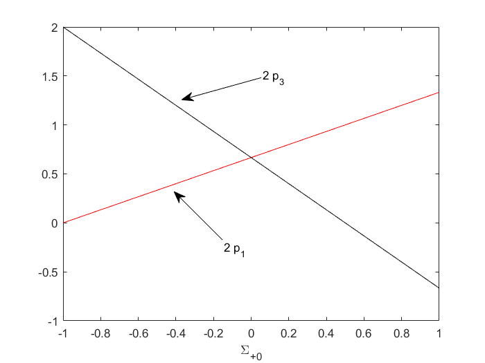
p1\displaystyle p_{1} =13​(1+Σ+0+3​Σ−0),\displaystyle=\frac{1}{3}(1+\Sigma_{+0}+\sqrt{3}\Sigma_{-0}), (2)
p2\displaystyle p_{2} =13​(1+Σ+0−3​Σ−0),\displaystyle=\frac{1}{3}(1+\Sigma_{+0}-\sqrt{3}\Sigma_{-0}), (3)
p3\displaystyle p_{3} =13​(1−2​Σ+0).\displaystyle=\frac{1}{3}(1-2\Sigma_{+0}). (4)

The non-zero Hubble-normalised shear components are Σ+0\Sigma_{+0} and Σ−0\Sigma_{-0}, and they are constant, with Σ+02+Σ−02≤1\Sigma_{+0}^{2}+\Sigma_{-0}^{2}\leq 1. The stiff fluid has pressure pp and density ρ\rho given by

p=ρ=1−Σ+02−Σ−023​t2.p=\rho=\frac{1-\Sigma_{+0}^{2}-\Sigma_{-0}^{2}}{3t^{2}}. (5)

To impose the LRS condition; it is simplest to set Σ−0=0\Sigma_{-0}=0, so the parameter Σ+0\Sigma_{+0} takes values from −1-1 to 11. Σ+0=−1\Sigma_{+0}=-1 gives the LRS Kasner solution [45, page 132] with (p1,p2,p3)=(0,0,1)(p_{1},p_{2},p_{3})=(0,0,1) (also known as the Taub form of flat spacetime); Σ+0=1\Sigma_{+0}=1 gives the LRS Kasner solution with (p1,p2,p3)=(23,23,−13)(p_{1},p_{2},p_{3})=(\frac{2}{3},\frac{2}{3},-\frac{1}{3}); Σ+0=0\Sigma_{+0}=0 gives the flat FLRW solution with stiff fluid.

The LRS Jacobs solution admits four KVFs, namely

∂x,∂y,∂z,−y∂x+x∂y,\partial_{x},\quad\partial_{y},\quad\partial_{z},\quad-y\partial_{x}+x\partial_{y}, (6)

where the fourth one is rotational.
We intend to apply the Stephani transformation with the general linear combination of the KVFs:

c1∂x+c2∂y+c3∂z+c4(−y∂x+x∂y)=(c1−c4y)∂x+(c2+c4x)∂y+c3∂zc_{1}\partial_{x}+c_{2}\partial_{y}+c_{3}\partial_{z}+c_{4}(-y\partial_{x}+x\partial_{y})=(c_{1}-c_{4}y)\partial_{x}+(c_{2}+c_{4}x)\partial_{y}+c_{3}\partial_{z} (7)

Observe that c1c_{1} and c2c_{2} can be eliminated without loss of generality by a translation in xx and yy directions. We set c4=1c_{4}=1 and c3=kc_{3}=k, so the KVF reads

−y∂x+x∂y+k∂z.-y\partial_{x}+x\partial_{y}+k\partial_{z}. (8)

This KVF forms an Abelian OT G2G_{2} group with exactly one other KVF (namely a linear combination of ∂z\partial_{z} and −y∂x+x∂y-y\partial_{x}+x\partial_{y}). By Geroch’s theorem [33, Appendix B], the generated metric will admit an Abelian OT G2G_{2} group.

There is a rotational symmetry about the zz-axis, so we adopt cylindrical coordinates (r,ψ,z)(r,\psi,z), but we want to arrange the coordinates in the following order: (t,ψ,z,r)(t,\psi,z,r), due to the way we adapt the orthonormal frame to the coordinates. In these coordinates, the KVF reads

∂ψ+k∂z.\partial_{\psi}+k\partial_{z}. (9)

We want to simplify the KVF to just ∂ψ\partial_{\psi} for the application of the Stephani transformation, so we make a further change of coordinates, by introducing

Z=z−k​ψ.Z=z-k\psi. (10)

Then, in the coordinates (t,ψ,Z,r)(t,\psi,Z,r), the KVF is simply ∂ψ\partial_{\psi}, but the line element now reads

d​s2\displaystyle ds^{2} =−d​t2+(k2​t2​p3+r2​t2​p1)​d​ψ2+2​k​t2​p3​d​ψ​d​Z+t2​p3​d​Z2+t2​p1​d​r2.\displaystyle=-dt^{2}+(k^{2}t^{2p_{3}}+r^{2}t^{2p_{1}})d\psi^{2}+2kt^{2p_{3}}d\psi dZ+t^{2p_{3}}dZ^{2}+t^{2p_{1}}dr^{2}. (11)

This shall be the seed solution to which we apply the Stephani transformation. It has the simple form (88). For later convenience we list the bb’s and nn’s of this line element and define the squared norm of the KVF below.

λ=k2​t2​p3+r2​t2​p1,\lambda=k^{2}t^{2p_{3}}+r^{2}t^{2p_{1}}, (12)
N\displaystyle N =1\displaystyle=1 (13)
b1\displaystyle b^{1} =−12​ln⁡λ\displaystyle=-\frac{1}{2}\ln\lambda (14)
b2\displaystyle b^{2} =−12​ln⁡r2​t2​p1+2​p3λ\displaystyle=-\frac{1}{2}\ln\dfrac{r^{2}t^{2p_{1}+2p_{3}}}{\lambda} (15)
b3\displaystyle b^{3} =−12​ln⁡(t2​p1)\displaystyle=-\frac{1}{2}\ln(t^{2p_{1}}) (16)
n1\displaystyle n_{1} =k​t2​p3λ\displaystyle=\frac{kt^{2p_{3}}}{\lambda} (17)
n2\displaystyle n_{2} =0=n3.\displaystyle=0=n_{3}. (18)

Observe that

b1+b2+b3=−ln⁡(r​t).b^{1}+b^{2}+b^{3}=-\ln(rt). (19)

The ψ\psi-ZZ area element

𝒜=e−b1−b2=r​tp1+p3\mathcal{A}=e^{-b^{1}-b^{2}}=rt^{p_{1}+p_{3}} (20)

and volume element

𝒱=e−b1−b2−b3=r​t\mathcal{V}=e^{-b^{1}-b^{2}-b^{3}}=rt (21)

are always expanding.

Here we list the dynamical variables of the seed solution using the formulas in Appendix A. To write the expressions in a more compact form, we list several intermediate expressions, particularly the partial derivatives of the essential variable.

∂0λ\displaystyle\partial_{0}\lambda =2​p3​k2​t2​p3−1+2​p1​r2​t2​p1−1\displaystyle=2p_{3}k^{2}t^{2p_{3}-1}+2p_{1}r^{2}t^{2p_{1}-1} (22)
∂3λ\displaystyle\partial_{3}\lambda =2​r​t2​p1\displaystyle=2rt^{2p_{1}} (23)

So the expressions are

H\displaystyle H =13​t\displaystyle=\frac{1}{3t} (24)
Θ11\displaystyle\Theta_{11} =12​(∂0λλ)\displaystyle=\frac{1}{2}\left(\frac{\partial_{0}\lambda}{\lambda}\right) (25)
Θ22\displaystyle\Theta_{22} =12​(2​p1+2​p3t−∂0λλ)\displaystyle=\frac{1}{2}\left(\frac{2p_{1}+2p_{3}}{t}-\frac{\partial_{0}\lambda}{\lambda}\right) (26)
Θ33\displaystyle\Theta_{33} =12​(2​p1t)\displaystyle=\frac{1}{2}\left(\frac{2p_{1}}{t}\right) (27)
Θ12\displaystyle\Theta_{12} =12​k​t−p1+p3r​(−∂0λλ+2​p3t)\displaystyle=\frac{1}{2}\dfrac{kt^{-p_{1}+p_{3}}}{r}\left(-\frac{\partial_{0}\lambda}{\lambda}+2\frac{p_{3}}{t}\right) (28)
u˙3\displaystyle\dot{u}_{3} =0\displaystyle=0 (29)
n11\displaystyle n_{11} =k​t−2​p1+p3r​(−∂3λλ)\displaystyle=\dfrac{kt^{-2p_{1}+p_{3}}}{r}\left(-\frac{\partial_{3}\lambda}{\lambda}\right) (30)
n12\displaystyle n_{12} =12​t−p1​(1r−∂3λλ)\displaystyle=\frac{1}{2}t^{-p_{1}}\left(\frac{1}{r}-\frac{\partial_{3}\lambda}{\lambda}\right) (31)
a3\displaystyle a_{3} =−12​t−p1r\displaystyle=-\frac{1}{2}\dfrac{t^{-p_{1}}}{r} (32)
Σ11\displaystyle\Sigma_{11} =32​(t​∂0λλ)−1\displaystyle=\frac{3}{2}\left(\frac{t\partial_{0}\lambda}{\lambda}\right)-1 (33)
Σ22\displaystyle\Sigma_{22} =32​(2​p1+2​p3−t​∂0λλ)−1\displaystyle=\frac{3}{2}\left({2p_{1}+2p_{3}}-\frac{t\partial_{0}\lambda}{\lambda}\right)-1 (34)
Σ33\displaystyle\Sigma_{33} =3​p1−1\displaystyle=3p_{1}-1 (35)
Σ12\displaystyle\Sigma_{12} =32​k​t1−p1+p3r​(−∂0λλ+2​p3t).\displaystyle=\frac{3}{2}\dfrac{kt^{1-p_{1}+p_{3}}}{r}\left(-\frac{\partial_{0}\lambda}{\lambda}+2\frac{p_{3}}{t}\right). (36)

Define Hubble-normalised expansion shear components Σ+\Sigma_{+} and Σ−\Sigma_{-} as

Σ+\displaystyle\Sigma_{+} =−12​Σ33\displaystyle=-\frac{1}{2}\Sigma_{33} (37)
Σ−\displaystyle\Sigma_{-} =Σ11−Σ222​3,\displaystyle=\frac{\Sigma_{11}-\Sigma_{22}}{2\sqrt{3}}, (38)

which gives

Σ+\displaystyle\Sigma_{+} =−12​Σ+0\displaystyle=-\frac{1}{2}\Sigma_{+0} (39)
Σ−\displaystyle\Sigma_{-} =32​(t​(ln⁡λ)t−2−Σ+03).\displaystyle=\frac{\sqrt{3}}{2}\left(t(\ln\lambda)_{t}-\frac{2-\Sigma_{+0}}{3}\right). (40)

Figure 1 shows that state space orbits projected on the (Σ+,Σ−)(\Sigma_{+},\Sigma_{-}) plane for various values of Σ+0\Sigma_{+0}. The r=0r=0 orbits are fixed points. r≠0r\neq 0 orbits move away from these fixed points as tt increases but only in Σ−\Sigma_{-} direction.

Refer to caption
Figure 1: State space orbits projected on the (Σ+,Σ−)(\Sigma_{+},\Sigma_{-}) plane for various values of Σ+0\Sigma_{+0}. A circle represents the orbit along r=0r=0, which is a fixed point. At tt increases, r≠0r\neq 0 orbits move away from these fixed points for Σ+0>0\Sigma_{+0}>0, and towards these fixed points Σ+0<0\Sigma_{+0}<0.

The solution is undefined at r=0r=0 if k=0k=0 (coordinate singularity). It is straightforward to analyse l=t​(ln⁡λ)tl=t(\ln\lambda)_{t}. If k=0k=0 then l=2​p1l=2p_{1}. If k≠0k\neq 0, then l=2​p3l=2p_{3} at r=0r=0. For r≠0r\neq 0 write

l=p3​(1−τ)+p1​(1+τ),τ=tanh⁡(Σ+0​(ln⁡t)+ln⁡|k|−ln⁡r).l=p_{3}(1-\tau)+p_{1}(1+\tau),\quad\tau=\tanh(\Sigma_{+0}(\ln t)+\ln|k|-\ln r). (41)

For Σ+0>0\Sigma_{+0}>0, ll goes from 2​p32p_{3} to 2​p12p_{1} as tt goes from 00 (early times) to ∞\infty (late times). For Σ+0<0\Sigma_{+0}<0, ll goes from 2​p12p_{1} to 2​p32p_{3}. For Σ+0=0\Sigma_{+0}=0, l=23l=\frac{2}{3}. So ll has a simple sigmoid transitional dynamics. It has a discontinuous limit along r=0r=0 (at late times for Σ+0>0\Sigma_{+0}>0, at early times for Σ+0<0\Sigma_{+0}<0). We take this opportunity to introduce the transition time, which roughly means when the transition occurs. For ll we define the transition time to be τ=0\tau=0, that is when

Σ+0​ln⁡t+ln⁡|k|−ln⁡r=0,\Sigma_{+0}\ln t+\ln|k|-\ln r=0, (42)

or equivalently when the two competing terms in λ\lambda are equal. Solving for tt gives the transition time

t=(r|k|)−1Σ+0.t=\left(\frac{r}{|k|}\right)^{-\frac{1}{\Sigma_{+0}}}. (43)

From (41), observe that Σ+0\Sigma_{+0} appears as the coefficient of ln⁡t\ln t in the tanh\tanh function. So smaller |Σ+0||\Sigma_{+0}| leads to milder slope/longer transition duration.
To summarise, the seed solution (11) has permanent false spikes in the case k≠0k\neq 0:
1. At r=0r=0 at late times for 0<Σ+0≤10<\Sigma_{+0}\leq 1.
2. At r=0r=0 at early times for −1≤Σ+0<0-1\leq\Sigma_{+0}<0.
If k=0k=0, the seed solution has no false spikes.

In the next two chapters we apply the Stephani transformation on this seed solution.

Chapter 3 Generated Solution, k=0k=0

In this chapter, we apply Stephani transformation on the seed solution (11) for the case k=0k=0 (that is, using only the rotational KVF) and discuss the dynamics of the generated solution. Computation is carried out using Maple.

1 Applying the Stephani transformation

We now carry out the Stephani transformation with the rotational KVF ∂ψ\partial_{\psi}. First we find the squared norm of the KVF,

λ=r2​t2​p1,\lambda=r^{2}t^{2p_{1}}, (1)

and the twist of the KVF,

ω\displaystyle\omega =ω0.\displaystyle=\omega_{0}. (2)

The combination λ2+ω2\lambda^{2}+\omega^{2} will appear frequently, so for brevity we introduce

F=λ2+ω2.F=\lambda^{2}+\omega^{2}. (3)

The next step is to find a particular solution βa\beta_{a} for the constrained system

∇[aβb]=2λ∇aξb+ωϵa​b​c​d∇cξd,ξaβa=F−1.\nabla_{[a}\beta_{b]}=2\lambda\nabla_{a}\xi_{b}+\omega\epsilon_{abcd}\nabla^{c}\xi^{d},\quad{\xi^{a}\beta_{a}=F-1}. (4)

We obtain

βa=(0,F−1,β2,0),\beta_{a}=(0,F-1,\beta_{2},0), (5)

where

β2=2​p1​ω0​r2+4​ω01+p3​t1+p3\displaystyle\beta_{2}=2p_{1}\omega_{0}r^{2}+\frac{4\omega_{0}}{1+p_{3}}t^{1+p_{3}} (6)

is found by integration.

The generated metric is then given through bb’s and nn’s by the formulas (94)–(100), dropping tildes for brevity.

N\displaystyle N =F1/2\displaystyle=F^{1/2} (7)
b1\displaystyle b^{1} =−12​ln⁡λF\displaystyle=-\frac{1}{2}\ln\frac{\lambda}{F} (8)
b2\displaystyle b^{2} =−12​ln⁡F​r2​t2​p1+2​p3λ\displaystyle=-\frac{1}{2}\ln\dfrac{Fr^{2}t^{2p_{1}+2p_{3}}}{\lambda} (9)
b3\displaystyle b^{3} =−12​ln⁡(F​t2​p1)\displaystyle=-\frac{1}{2}\ln(Ft^{2p_{1}}) (10)
n1\displaystyle n_{1} =−β2\displaystyle=-\beta_{2} (11)
n2\displaystyle n_{2} =0\displaystyle=0 (12)
n3\displaystyle n_{3} =0.\displaystyle=0. (13)

Observe that

b1+b2+b3=−12​ln⁡(F​r2​t4​p1+2​p3)=−12​ln⁡(F​r2​t2).b^{1}+b^{2}+b^{3}=-\frac{1}{2}\ln(Fr^{2}t^{4p_{1}+2p_{3}})=-\frac{1}{2}\ln(Fr^{2}t^{2}). (14)

2 The dynamical variables

Here we list the dynamical variables of the generated solution using the formulas in Appendix A. To write the expressions in a more compact form, we list several intermediate expressions, particularly the partial derivatives of the essential variables.

∂0λ=2​p1​r2​t2​p1−1\partial_{0}\lambda=2p_{1}r^{2}t^{2p_{1}-1} (15)
∂3λ=2​r​t2​p1\partial_{3}\lambda=2rt^{2p_{1}} (16)
∂0ω=0\partial_{0}\omega=0 (17)
∂3ω=0\partial_{3}\omega=0 (18)
∂0F=2​λ​∂0λ+2​ω​∂0ω\partial_{0}F=2\lambda\partial_{0}\lambda+2\omega\partial_{0}\omega (19)
∂3F=2​λ​∂3λ+2​ω​∂3ω\partial_{3}F=2\lambda\partial_{3}\lambda+2\omega\partial_{3}\omega (20)
∂0β2=4​ω​tp3\partial_{0}\beta_{2}=4\omega t^{p_{3}} (21)
∂3β2=4​p1​ω​r.\partial_{3}\beta_{2}=4{p_{1}}\omega r. (22)

Now using the above convention, we get

H\displaystyle H =16F−1/2(∂0FF+2t)\displaystyle=\frac{1}{6}F^{-1/2}\left(\frac{\partial_{0}F}{F}+\frac{2}{t}\right) (23)
Θ11\displaystyle\Theta_{11} =12F−1/2(∂0λλ−∂0FF)\displaystyle=\frac{1}{2}F^{-1/2}\left(\frac{\partial_{0}\lambda}{\lambda}-\frac{\partial_{0}F}{F}\right) (24)
Θ22\displaystyle\Theta_{22} =12F−1/2(∂0FF−∂0λλ+2​p1+2​p3t)\displaystyle=\frac{1}{2}F^{-1/2}\left(\frac{\partial_{0}F}{F}-\frac{\partial_{0}\lambda}{\lambda}+\frac{2p_{1}+2p_{3}}{t}\right) (25)
Θ33\displaystyle\Theta_{33} =12F−1/2(∂0FF+2​p1t)\displaystyle=\frac{1}{2}F^{-1/2}\left(\frac{\partial_{0}F}{F}+\frac{2p_{1}}{t}\right) (26)
Θ12\displaystyle\Theta_{12} =λ​t−p1−p32​r​F3/2​∂0β2\displaystyle=\dfrac{\lambda t^{-p_{1}-p_{3}}}{2rF^{3/2}}{\partial_{0}\beta_{2}} (27)
u˙3\displaystyle\dot{u}_{3} =−12F−1/2t−p1(∂3FF)\displaystyle=-\frac{1}{2}F^{-1/2}t^{-p_{1}}\left(\frac{\partial_{3}F}{F}\right) (28)
n11\displaystyle n_{11} =−λ​t−2​p1−p3r​F3/2∂3β2\displaystyle=-\dfrac{\lambda t^{-2p_{1}-p_{3}}}{rF^{3/2}}{\partial_{3}\beta_{2}} (29)
n12\displaystyle n_{12} =12F−1/2t−p1(∂3FF−∂3λλ+1r)\displaystyle=\frac{1}{2}{F^{-1/2}t^{-p_{1}}}\left(\dfrac{\partial_{3}F}{F}-\frac{\partial_{3}\lambda}{\lambda}+\frac{1}{r}\right) (30)
a3\displaystyle a_{3} =−12​F−1/2t−p1r.\displaystyle=-\frac{1}{2}\dfrac{F^{-1/2}t^{-p_{1}}}{r}. (31)

3 Dynamics of the solution

The state space orbits of a solution, projected onto the (Σ+,Σ−)(\Sigma_{+},\Sigma_{-}) plane, can provide some insight into the dynamics of the solution. Recall that (Σ+,Σ−)(\Sigma_{+},\Sigma_{-}) are defined in terms of the diagonal components of the Hubble-normalised expansion shear as

Σ+\displaystyle\Sigma_{+} =−12​Σ33,\displaystyle=-\frac{1}{2}\Sigma_{33}, (32)
Σ−\displaystyle\Sigma_{-} =Σ11−Σ222​3.\displaystyle=\frac{\Sigma_{11}-\Sigma_{22}}{2\sqrt{3}}. (33)

This reduces to

Σ+=−Σ+0+f2+f,Σ−=3​(Σ+0−f)2+f,\Sigma_{+}=-\frac{\Sigma_{+0}+f}{2+f},\quad\Sigma_{-}=\frac{\sqrt{3}(\Sigma_{+0}-f)}{2+f}, (34)

where

f=t​(ln⁡F)t=4​p1​r4​t4​p1r4​t4​p1+ω02,p1=13​(1+Σ+0).f=t(\ln F)_{t}=\frac{4p_{1}r^{4}t^{4p_{1}}}{r^{4}t^{4p_{1}}+\omega_{0}^{2}},\ \ \ p_{1}=\frac{1}{3}(1+\Sigma_{+0}). (35)

We carry out the asymptotic analysis of ff, similar to what we did for ll in Chapter 3.

1 Case ω0≠0\omega_{0}\neq 0

Along r=0r=0, we have f=0f=0 and

(Σ+,Σ−)=(−12​Σ+0,32​Σ+0).\displaystyle(\Sigma_{+},\Sigma_{-})=(-\frac{1}{2}\Sigma_{+0},\frac{\sqrt{3}}{2}\Sigma_{+0}). (36)

Along r≠0r\neq 0, provided that p1≠0p_{1}\neq 0, we have

f→{0ast→04​p1ast→∞,\displaystyle f\rightarrow\begin{cases}0&\text{as}\ \ \ t\rightarrow 0\\ 4p_{1}&\text{as}\ \ \ t\rightarrow\infty,\end{cases} (37)

and

(Σ+,Σ−)→{(−12​Σ+0,32​Σ+0)ast→0(−(7​Σ+0+4)2​(2​Σ+0+5),−3​(4+Σ+0)2​(2​Σ+0+5))ast→∞.\displaystyle(\Sigma_{+},\Sigma_{-})\rightarrow\begin{cases}(-\frac{1}{2}\Sigma_{+0},\frac{\sqrt{3}}{2}\Sigma_{+0})&\text{as}\ \ \ t\rightarrow 0\\ (-\frac{(7\Sigma_{+0}+4)}{2(2\Sigma_{+0}+5)},-\frac{\sqrt{3}(4+\Sigma_{+0})}{2(2\Sigma_{+0}+5)})&\text{as}\ \ \ t\rightarrow\infty.\end{cases} (38)

There is a permanent spike at r=0r=0 at late times, for p1≠0p_{1}\neq 0 ⇔\Leftrightarrow Σ+0>−1\Sigma_{+0}>-1.

Refer to caption
Figure 1: State space orbits projected on the (Σ+,Σ−)(\Sigma_{+},\Sigma_{-}) plane for various values of Σ+0\Sigma_{+0} for ω0≠0\omega_{0}\neq 0. A circle represents the orbit along r=0r=0, which is a fixed point. r≠0r\neq 0 orbits move away from these fixed points as tt increases, mimicking the orbits of Taub solutions.

Figure 1 shows the state space orbits projected on the (Σ+,Σ−)(\Sigma_{+},\Sigma_{-}) plane for various values of Σ+0\Sigma_{+0} for ω0≠0\omega_{0}\neq 0. The r=0r=0 orbits are fixed points, while the r≠0r\neq 0 orbits move away from these fixed points as tt increases, mimicking the orbits of Taub solutions [45, page 136].

The exceptional case is when Σ+0=−1\Sigma_{+0}=-1, where (Σ+,Σ−)=(12,−32)(\Sigma_{+},\Sigma_{-})=(\frac{1}{2},-\frac{\sqrt{3}}{2}) for all tt and rr. But this is not a Kasner solution. Recall that the timelike KVF is preserved. The Weyl scalars (see Appendix C) are time-independent :

C​C\displaystyle CC =−(192​(−r12+15​ω02​r8−15​ω04​r4+ω06))(r4+ω02)6\displaystyle=-\frac{(192(-r^{12}+15\omega_{0}^{2}r^{8}-15\omega_{0}^{4}r^{4}+\omega_{0}^{6}))}{(r^{4}+\omega_{0}^{2})^{6}} (39)
C​C​s\displaystyle CCs =−384​ω0​r2​(−r4+3​ω02)​(−3​r4+ω02)(r4+ω02)6\displaystyle=-\frac{384\omega_{0}r^{2}(-r^{4}+3\omega_{0}^{2})(-3r^{4}+\omega_{0}^{2})}{(r^{4}+\omega_{0}^{2})^{6}} (40)
C​C​C\displaystyle CCC =−768​r2​(−r4+3​ω02)​(−r12+33​ω02​r8−27​ω04​r4+3​ω06)(r4+ω02)9\displaystyle=-\frac{768r^{2}(-r^{4}+3\omega_{0}^{2})(-r^{12}+33\omega_{0}^{2}r^{8}-27\omega_{0}^{4}r^{4}+3\omega_{0}^{6})}{(r^{4}+\omega_{0}^{2})^{9}} (41)
C​C​C​s\displaystyle CCCs =768​ω0​(−3​r4+ω02)​(−3​r12+27​ω02​r8−33​ω04​r4+ω06)(r4+ω02)9.\displaystyle=\frac{768\omega_{0}(-3r^{4}+\omega_{0}^{2})(-3r^{12}+27\omega_{0}^{2}r^{8}-33\omega_{0}^{4}r^{4}+\omega_{0}^{6})}{(r^{4}+\omega_{0}^{2})^{9}}. (42)

The inhomogeneities do not become narrow, so there are no spikes. Figure 2 shows the snapshots of Ωk\Omega_{k} and Σ2\Sigma^{2}, whose amplitude increases indefinitely, but whose width is constant.

Refer to caption
(a) Ωk\Omega_{k}
Refer to caption
(b) Σ2\Sigma^{2}
Figure 2: Snapshots of Ωk\Omega_{k} and Σ2\Sigma^{2} for ω0=1\omega_{0}=1 and Σ+0=−1\Sigma_{+0}=-1, showing that the inhomogeneities do not become narrow.

2 Case ω0=0\omega_{0}=0

In this case (35) reduces to f=4​p1f=4p_{1}, and (34) simplifies to

Σ+\displaystyle\Sigma_{+} =−7​Σ+0+42​(2​Σ+0+5),\displaystyle=-\frac{7\Sigma_{+0}+4}{2(2\Sigma_{+0}+5)}, Σ−=−3​(Σ+0+4)2​(2​Σ+0+5).\displaystyle\Sigma_{-}=-\frac{\sqrt{3}(\Sigma_{+0}+4)}{2(2\Sigma_{+0}+5)}. (43)

From the fluid density

ρ=1−Σ+023​r4​t2+4​p1\rho=\frac{1-\Sigma_{+0}^{2}}{3r^{4}t^{2+4p_{1}}} (44)

we conclude that for −1<Σ+0<1-1<\Sigma_{+0}<1 a physical singularity exists at r=0r=0.

For the vacuum cases Σ+0=±1\Sigma_{+0}=\pm 1, we can reach the same conclusion by examining the Weyl scalars. For Σ+0=−1\Sigma_{+0}=-1 we have 11 1 This solution is equivalent to a Kasner solution (in the broader sense), or a Levi-Civita solution [44, pages 197 and 343].

C​C\displaystyle CC =192r12\displaystyle=\frac{192}{r^{12}} (45)
C​C​s\displaystyle CCs =0\displaystyle=0 (46)
C​C​C\displaystyle CCC =−768r18\displaystyle=-\frac{768}{r^{18}} (47)
C​C​C​s\displaystyle CCCs =0.\displaystyle=0. (48)

And for Σ+0=1\Sigma_{+0}=1 we have

C​C\displaystyle CC =64​(7​r4−18​r2​t2/3+27​t4/3)9​r12​t28/3\displaystyle=\frac{64(7r^{4}-18r^{2}t^{2/3}+27t^{4/3})}{9r^{12}t^{28/3}} (49)
C​C​s\displaystyle CCs =0\displaystyle=0 (50)
C​C​C\displaystyle CCC =256​(r6​t2/3−5​r4​t4/3+9​r2​t2−9​t8/3)3​r18​t44/3\displaystyle=\frac{256(r^{6}t^{2/3}-5r^{4}t^{4/3}+9r^{2}t^{2}-9t^{8/3})}{3r^{18}t^{44/3}} (51)
C​C​C​s\displaystyle CCCs =0.\displaystyle=0. (52)

Because there is a physical singularity at r=0r=0, we should not say that a spike occurs there.

4 Radius of spike

Following [25], we define the coordinate radius of spike (or inhomogeneities) to be the value of rr where

λ=|ω|,\lambda=|\omega|, (53)

which gives

coordinate radius=|ω0|​t−13​(1+Σ+0).\text{coordinate radius}=\sqrt{|\omega_{0}|}t^{-\frac{1}{3}(1+\Sigma_{+0})}. (54)

For Σ+0=−1\Sigma_{+0}=-1 the coordinate radius is constant (so the inhomogeneities cannot be called as spike).

For Σ+0>−1\Sigma_{+0}>-1, the coordinate radius tends to zero as t→∞t\rightarrow\infty, indicating the formation of permanent spike along r=0r=0 at late times.

We must measure the radius of the spike with respect to some important scale like horizon – the particle or event horizon. From (89) and (11), we obtain

coordinate radius of particle horizon =∫0tNg33 dt\displaystyle=\int_{0}^{t}\frac{N}{\sqrt{g_{33}}}\text{ }dt (55)
=∫0tt−13​(1+Σ+0) dt\displaystyle=\int_{0}^{t}t^{-\frac{1}{3}(1+\Sigma_{+0})}\text{ }dt (56)
=32−Σ+0​t13​(2−Σ+0)\displaystyle=\frac{3}{2-\Sigma_{+0}}t^{\frac{1}{3}(2-\Sigma_{+0})} (57)

Their ratio is

coordinate radius of spikecoordinate radius of particle horizon=(2−Σ+03)​|ω0|​t−1.\frac{\text{coordinate radius of spike}}{\text{coordinate radius of particle horizon}}=\left(\frac{2-\Sigma_{+0}}{3}\right)\sqrt{|\omega_{0}|}t^{-1}. (58)

The physical radius of the spike is

s=∫0coordinate radius of spikegr​r dr.s=\int_{0}^{\text{coordinate radius of spike}}\sqrt{g_{rr}}\text{ }dr. (59)

where

gr​r=F​t2​p1.\sqrt{g_{rr}}=\sqrt{Ft^{2p_{1}}}.\\ (60)

Let

u\displaystyle u =r​t13+13​Σ+0|ω0|12\displaystyle=\frac{rt^{\frac{1}{3}+\frac{1}{3}\Sigma_{+0}}}{|\omega_{0}|^{\frac{1}{2}}} and du=t13+13​Σ+0|ω0|12 dr\displaystyle du=\frac{t^{\frac{1}{3}+\frac{1}{3}\Sigma_{+0}}}{|\omega_{0}|^{\frac{1}{2}}}\text{ }dr (61)

and the limits are u=0u=0 and 11. Then

s=|ω0|3/2∫011+u4 du.s=|\omega_{0}|^{3/2}\int_{0}^{{1}}\sqrt{1+u^{4}}\text{ }du. (62)

i.e. the physical radius of the spike is constant. As the universe expands, in comparison the spike becomes narrower and narrower.

5 Discussion

We set out to generate a solution with a permanent spike that forms at late times. We have achieved this by applying the Stephani transformation on the LRS Jacobs solution, using the rotational KVF. The generated solution is cylindrically symmetric, and has a spike along its rotational axis for the case Σ+0>−1\Sigma_{+0}>-1, ω0≠0\omega_{0}\neq 0. This is the first generated solution with a late-time permanent spike, and the first generated solution with a spike along a line.22 2 Such features can also be achieved through silent LTB and Szekeres models [6] without using solution-generating transformations. The spike produces an overdensity along the axis at late times, which is conducive to large scale structure formation. Thus the generated solution can serve as a prototypical model for formation of galactic filaments along web-like strings.

Chapter 4 Generated solutions, k≠0k\neq 0

In the previous chapter we have discussed the dynamics of generated solution for the case k=0k=0. We have seen the spike at late times.
In this chapter we are going to generalise the result to the case k≠0k\neq 0 (that is, using the general linear combination of KVFs).

1 Applying the Stephani transformation

We now carry out the Stephani transformation with the general KVF ∂ψ\partial_{\psi}. First we find the squared norm of the KVF,

λ=k2​t2​p3+r2​t2​p1,\lambda=k^{2}t^{2p_{3}}+r^{2}t^{2p_{1}}, (1)

and the twist of the KVF,

ω=2​k1+p3​t1+p3+k​Σ+0​r2+ω0.\displaystyle\omega=\dfrac{2k}{1+p_{3}}t^{1+p_{3}}+k\Sigma_{+0}r^{2}+\omega_{0}. (2)

The combination λ2+ω2\lambda^{2}+\omega^{2} will appear frequently, so for brevity we introduce

F=λ2+ω2.F=\lambda^{2}+\omega^{2}. (3)

The next step is to find a particular solution βa\beta_{a} for the constrained system

∇[aβb]=2λ∇aξb+ωϵa​b​c​d∇cξd,ξaβa=F−1.\nabla_{[a}\beta_{b]}=2\lambda\nabla_{a}\xi_{b}+\omega\epsilon_{abcd}\nabla^{c}\xi^{d},\quad{\xi^{a}\beta_{a}=F-1}. (4)

We obtain

βa=(0,F−1,β2,0),\beta_{a}=(0,F-1,\beta_{2},0), (5)

where

β2=2​p1​ω0​r2+p1​Σ+0​k​r4+(4​ω+2​k​(1−p3)​r21+p3)​t1+p3+k3​t4​p3+4​k(1+p3)2​t2+2​p3\displaystyle\beta_{2}=2p_{1}\omega_{0}r^{2}+p_{1}\Sigma_{+0}kr^{4}+\left(\frac{4\omega+2k(1-p_{3})r^{2}}{1+p_{3}}\right)t^{1+p_{3}}+k^{3}t^{4p_{3}}+\frac{4k}{(1+p_{3})^{2}}t^{2+2p_{3}} (6)

The generated metric is then given through bb’s and nn’s by the formulas (94)–(100), dropping tildes for brevity.

N\displaystyle N =F1/2\displaystyle=F^{1/2} (7)
b1\displaystyle b^{1} =−12​ln⁡λF\displaystyle=-\frac{1}{2}\ln\frac{\lambda}{F} (8)
b2\displaystyle b^{2} =−12​ln⁡F​r2​t2​p1+2​p3λ\displaystyle=-\frac{1}{2}\ln\dfrac{Fr^{2}t^{2p_{1}+2p_{3}}}{\lambda} (9)
b3\displaystyle b^{3} =−12​ln⁡(F​t2​p1)\displaystyle=-\frac{1}{2}\ln(Ft^{2p_{1}}) (10)
n1\displaystyle n_{1} =F​k​t2​p3λ−β2\displaystyle=\frac{Fkt^{2p_{3}}}{\lambda}-\beta_{2} (11)
n2\displaystyle n_{2} =0\displaystyle=0 (12)
n3\displaystyle n_{3} =0.\displaystyle=0. (13)

Its ψ\psi-ZZ area element

𝒜=r​tp1+p3\mathcal{A}=rt^{p_{1}+p_{3}} (14)

is the same as the seed solution’s, and is always expanding. Its volume element

𝒱=r​t​F\mathcal{V}=rt\sqrt{F} (15)

is different from the seed solution’s and is not always expanding. This means the Hubble scalar HH can become negative for some parameter values, and Hubble-normalised variables would blow up. In this case we use β\beta-normalisation, which is based on the ever-expanding area element [46].

2 The dynamical variables

Here we list the dynamical variables of the generated solution using the formulas in Appendix A. To write the expressions in a more compact form, we list several intermediate expressions, particularly the partial derivatives of the essential variables.

∂0λ\displaystyle\partial_{0}\lambda =2​p3​k2​t2​p3−1+2​p1​r2​t2​p1−1\displaystyle=2p_{3}k^{2}t^{2p_{3}-1}+2p_{1}r^{2}t^{2p_{1}-1} (16)
∂3λ\displaystyle\partial_{3}\lambda =2​r​t2​p1\displaystyle=2rt^{2p_{1}} (17)
∂0ω\displaystyle\partial_{0}\omega =2​k​tp3\displaystyle=2kt^{p_{3}} (18)
∂3ω\displaystyle\partial_{3}\omega =2​k​(3​p1−1)​r\displaystyle=2k(3p_{1}-1)r (19)
∂0F\displaystyle\partial_{0}F =2​λ​∂0λ+2​ω​∂0ω\displaystyle=2\lambda\partial_{0}\lambda+2\omega\partial_{0}\omega (20)
∂3F\displaystyle\partial_{3}F =2​λ​∂3λ+2​ω​∂3ω\displaystyle=2\lambda\partial_{3}\lambda+2\omega\partial_{3}\omega (21)
∂0β2\displaystyle\partial_{0}\beta_{2} =4​k​p3​λ​t2​p3−1+4​ω​tp3\displaystyle=4kp_{3}\lambda t^{2p_{3}-1}+4\omega t^{p_{3}} (22)
∂3β2\displaystyle\partial_{3}\beta_{2} =4​p1​ω​r.\displaystyle=4{p_{1}}\omega r. (23)

By using the above convention, we get this list of dynamical variables.

H\displaystyle H =16F−1/2(∂0FF+2t)\displaystyle=\frac{1}{6}F^{-1/2}\left(\frac{\partial_{0}F}{F}+\frac{2}{t}\right) (24)
Θ11\displaystyle\Theta_{11} =12F−1/2(∂0λλ−∂0FF)\displaystyle=\frac{1}{2}F^{-1/2}\left(\frac{\partial_{0}\lambda}{\lambda}-\frac{\partial_{0}F}{F}\right) (25)
Θ22\displaystyle\Theta_{22} =12F−1/2(∂0FF−∂0λλ+2​p1+2​p3t)\displaystyle=\frac{1}{2}F^{-1/2}\left(\frac{\partial_{0}F}{F}-\frac{\partial_{0}\lambda}{\lambda}+\frac{2p_{1}+2p_{3}}{t}\right) (26)
Θ33\displaystyle\Theta_{33} =12F−1/2(∂0FF+2​p1t)\displaystyle=\frac{1}{2}F^{-1/2}\left(\frac{\partial_{0}F}{F}+\frac{2p_{1}}{t}\right) (27)
Θ12\displaystyle\Theta_{12} =12​kF−1/2t−p1+p3r​(∂0FF−∂0λλ+2​p3t)−λ​t−p1−p32​r​F3/2​∂0β2\displaystyle=\frac{1}{2}\dfrac{kF^{-1/2}t^{-p_{1}+p_{3}}}{r}\left(\dfrac{\partial_{0}F}{F}-\frac{\partial_{0}\lambda}{\lambda}+2\frac{p_{3}}{t}\right)-\dfrac{\lambda t^{-p_{1}-p_{3}}}{2rF^{3/2}}{\partial_{0}\beta_{2}} (28)
u˙3\displaystyle\dot{u}_{3} =−12F−1/2t−p1(∂3FF)\displaystyle=-\frac{1}{2}F^{-1/2}t^{-p_{1}}\left(\frac{\partial_{3}F}{F}\right) (29)
n11\displaystyle n_{11} =kF−1/2t−2​p1+p3r​(∂3FF−∂3λλ)−λ​t−2​p1−p3r​F3/2​∂3β2\displaystyle=\dfrac{kF^{-1/2}t^{-2p_{1}+p_{3}}}{r}\left(\dfrac{\partial_{3}F}{F}-\frac{\partial_{3}\lambda}{\lambda}\right)-\dfrac{\lambda t^{-2p_{1}-p_{3}}}{rF^{3/2}}{\partial_{3}\beta_{2}} (30)
n12\displaystyle n_{12} =12F−1/2t−p1(∂3FF−∂3λλ+1r)\displaystyle=\frac{1}{2}{F^{-1/2}t^{-p_{1}}}\left(\dfrac{\partial_{3}F}{F}-\frac{\partial_{3}\lambda}{\lambda}+\frac{1}{r}\right) (31)
a3\displaystyle a_{3} =−12​F−1/2t−p1r.\displaystyle=-\frac{1}{2}\dfrac{F^{-1/2}t^{-p_{1}}}{r}. (32)

3 Dynamics of the solution

Now we find Σ+\Sigma_{+} and Σ−\Sigma_{-} by using the equations (32), (33). We have

Σ+=−Σ+0+f2+f,Σ−=3​(l−f−13​(2−Σ+0))2+f\Sigma_{+}=-\frac{\Sigma_{+0}+f}{2+f},\\ \quad\Sigma_{-}=\frac{\sqrt{3}(l-f-\frac{1}{3}(2-\Sigma_{+0}))}{2+f} (33)

where f=t​(ln⁡F)tf=t(\ln F)_{t}, l=t​(ln⁡λ)tl=t(\ln\lambda)_{t}. The β\beta-normalised (Σ+,Σ−)(\Sigma_{+},\Sigma_{-}) are

Σ+=−Σ+0+f2−Σ+0Σ−=3​(l−f)2−Σ+0−13.\Sigma_{+}=-\frac{\Sigma_{+0}+f}{2-\Sigma_{+0}}\\ \quad\Sigma_{-}=\frac{\sqrt{3}(l-f)}{2-\Sigma_{+0}}-\frac{1}{\sqrt{3}}. (34)

We have analysed the asymptotic dynamics of ll in Chapter 3. Recall that ll has a false spike at r=0r=0 at late times for 0<Σ+0≤10<\Sigma_{+0}\leq 1, and at early times for −1≤Σ+0<0-1\leq\Sigma_{+0}<0. The asymptotic dynamics of ff can be analysed as follows. ff consists of terms involving λ\lambda and terms involving ω\omega. λ\lambda contains two different power terms, t2​p1t^{2p_{1}} and t2​p3t^{2p_{3}}; while ω\omega contains t1+p3t^{1+p_{3}} and constant. At late times, the term with the biggest exponent dominates; at early times the term with the smallest exponent dominates.
Refer to caption
(a) λ\lambda exponents
Refer to caption
(b) ω\omega exponents
Refer to caption
(c) Dominant exponents in ff at late times
Refer to caption
(d) Dominant exponents in ff at early times
Figure 1: Exponents in λ\lambda, ω\omega and ff. Dotted lines indicate the next dominant exponent.

Because ff has the form

f=t​(λ2)t+t​(ω2)tλ2+ω2,f=\frac{t(\lambda^{2})_{t}+t(\omega^{2})_{t}}{\lambda^{2}+\omega^{2}}, (35)

and λ2\lambda^{2} and ω2\omega^{2} are sums of power of tt, the asymptotic limits of ff are determined by coefficients of the dominant terms in the general case. When there are two equally dominant terms, care is taken to include all equally dominant terms. It turns out that

limt→∞f=\displaystyle\lim\limits_{t\rightarrow\infty}f= {4​p1for 12≤Σ+0≤12​(1+p3)for −1≤Σ+0≤12\displaystyle\begin{cases}4p_{1}&\text{for }\ \ \ \frac{1}{2}\leq\Sigma_{+0}\leq 1\\ 2(1+p_{3})&\text{for }\ \ \ -1\leq\Sigma_{+0}\leq\frac{1}{2}\end{cases} (36)

and

limt→0f=\displaystyle\lim\limits_{t\rightarrow 0}f= {4​p3for12≤Σ+0≤10for−1≤Σ+0≤12.\displaystyle\begin{cases}4p_{3}&\text{for}\ \ \ \frac{1}{2}\leq\Sigma_{+0}\leq 1\\ 0&\text{for}\ \ \ -1\leq\Sigma_{+0}\leq\frac{1}{2}.\end{cases} (37)

In some special cases, the coefficient of a dominant term can become zero. Then we find the next dominant term. These special cases are: r=0r=0, which kills the t2​p1t^{2p_{1}} term in λ\lambda, r=−ω0k​Σ+0r=\sqrt{\frac{-\omega_{0}}{k\Sigma_{+0}}}, which kills the constant term in ω\omega, and k=0k=0, which kills the t2​p3t^{2p_{3}} term. The case k=0k=0 has been dealt with in Chapter 4. Figure 1 shows the exponents in λ\lambda, ω\omega and ff.
Along r=0r=0,

limt→∞f=2​(1+p3)\displaystyle\lim\limits_{t\rightarrow\infty}f=2(1+p_{3}) for all−1≤Σ+0≤1.\displaystyle\ \ \text{for all}\ \ \ -1\leq\Sigma_{+0}\leq 1. (38)

Along r=−ω0k​Σ+0r=\sqrt{\frac{-\omega_{0}}{k\Sigma_{+0}}},

limt→0f=\displaystyle\lim\limits_{t\rightarrow 0}f= {4​p3for​ 0≤Σ+0≤14​p1for−1≤Σ+0≤0\displaystyle\begin{cases}4p_{3}&\text{for}\ \ \ 0\leq\Sigma_{+0}\leq 1\\ 4p_{1}&\text{for}\ \ -1\leq\Sigma_{+0}\leq 0\end{cases} (39)

In the very special case ω0=0=r\omega_{0}=0=r, ff is equal to 4.
In summary, ff has a spike at r=0r=0 at late times for 12<Σ+0≤1\frac{1}{2}<\Sigma_{+0}\leq 1, a spike at r=0r=0 at early times for Σ+0=−1\Sigma_{+0}=-1, ω0=0\omega_{0}=0, and a spike at r=−ω0k​Σ+0≠0r=\sqrt{\frac{-\omega_{0}}{k\Sigma_{+0}}}\neq 0 at early times for −1<Σ+0<0-1<\Sigma_{+0}<0, ω0​k>0\omega_{0}k>0, or 0<Σ+0<120<\Sigma_{+0}<\frac{1}{2}, ω0​k<0.\omega_{0}k<0.
Combining the effects of ff and ll, we see that (Σ+,Σ−)(\Sigma_{+},\Sigma_{-}) has a spike at r=0r=0 at late times for 0<Σ+0≤10<\Sigma_{+0}\leq 1, a spike at r=0r=0 at early times for −1<Σ+0<0-1<\Sigma_{+0}<0, and a spike at r=−ω0k​Σ+0≠0r=\sqrt{\frac{-\omega_{0}}{k\Sigma_{+0}}}\neq 0 at early times for −1<Σ+0<0-1<\Sigma_{+0}<0, ω0​k>0\omega_{0}k>0, or 0<Σ+0<120<\Sigma_{+0}<\frac{1}{2}, ω0​k<0\omega_{0}k<0. Later we will see that the spike caused by ll is not real.

1 At late times (t→∞)(t\rightarrow\infty)

For −1<Σ+0≤0-1<\Sigma_{+0}\leq 0, we do not have a spike.

(Σ+,Σ−)→(−8−Σ+02​(7−2​Σ+0),−3​(8−Σ+0)2​(7−2​Σ+0)).\displaystyle(\Sigma_{+},\Sigma_{-})\rightarrow\left(-\frac{8-\Sigma_{+0}}{2(7-2\Sigma_{+0})},-\frac{\sqrt{3}(8-\Sigma_{+0})}{2(7-2\Sigma_{+0})}\right). (40)

See Figure 2.

Refer to caption
(a) Σ+0=−1\Sigma_{+0}=-1
Refer to caption
(b) Σ+0=−0.5\Sigma_{+0}=-0.5
Refer to caption
(c) Σ+0=0\Sigma_{+0}=0
Figure 2: State space orbits projected on the (Σ+,Σ−)(\Sigma_{+},\Sigma_{-}) plane for k=1k=1, Σ+0=−1,−0.5,0\Sigma_{+0}=-1,-0.5,0 and ω0=1\omega_{0}=1. All orbits end up at the same point indicated by an asterisk.

For 0<Σ+0<0.50<\Sigma_{+0}<0.5, we have a spike at r=0r=0.

(Σ+,Σ−)→\displaystyle(\Sigma_{+},\Sigma_{-})\rightarrow {(−8−Σ+02​(7−2​Σ+0),−3​(8−7​Σ+0)2​(7−2​Σ+0))along ​r≠0(−8−Σ+02​(7−2​Σ+0),−3​(8−Σ+0)2​(7−2​Σ+0))along ​r=0.\displaystyle\begin{cases}\left(-\frac{8-\Sigma_{+0}}{2(7-2\Sigma_{+0})},-\frac{\sqrt{3}(8-7\Sigma_{+0})}{2(7-2\Sigma_{+0})}\right)&\text{along }r\neq 0\\ \left(-\frac{8-\Sigma_{+0}}{2(7-2\Sigma_{+0})},-\frac{\sqrt{3}(8-\Sigma_{+0})}{2(7-2\Sigma_{+0})}\right)&\text{along }r=0.\end{cases} (41)

See Figure 3. Later we will see that this spike is not real.

Refer to caption
(a) Combine for all values of rr
Refer to caption
(b) For r=−ω0k​Σ+0r=\sqrt{-\frac{\omega_{0}}{k\Sigma_{+0}}}
Refer to caption
(c) For r=0r=0
Refer to caption
(d) For a large value of rr
Figure 3: State space orbits for k=1k=1, Σ+0=0.25\Sigma_{+0}=0.25 and ω0=−1\omega_{0}=-1.

For Σ+0=0.5\Sigma_{+0}=0.5, we have a spike at r=0r=0.

(Σ+,Σ−)→\displaystyle(\Sigma_{+},\Sigma_{-})\rightarrow {(−58,−38​3)along ​r≠0(−58,−58​3)along ​r=0.\displaystyle\begin{cases}\left(-\frac{5}{8},-\frac{3}{8}\sqrt{3}\right)&\text{along }r\neq 0\\ \left(-\frac{5}{8},-\frac{5}{8}\sqrt{3}\right)&\text{along }r=0.\end{cases} (42)

See Figure 4. Later we will see that this spike is not real.

Refer to caption
(a) Combine for all values of rr
Refer to caption
(b) For r=−ω0k​Σ+0r=\sqrt{-\frac{\omega_{0}}{k\Sigma_{+0}}}
Refer to caption
(c) For r=0r=0
Refer to caption
(d) For a large value of rr
Figure 4: State space orbits for k=1k=1, Σ+0=0.5\Sigma_{+0}=0.5 and ω0=−1\omega_{0}=-1.

For 0.5<Σ+0≤10.5<\Sigma_{+0}\leq 1, we have a spike at r=0r=0

(Σ+,Σ−)→\displaystyle(\Sigma_{+},\Sigma_{-})\rightarrow {(−4+7​Σ+02​(5+2​Σ+0),−3​(4+Σ+0)2​(5+2​Σ+0))along ​r≠0(−8−Σ+02​(7−2​Σ+0),−3​(8−Σ+0)2​(7−2​Σ+0))along ​r=0.\displaystyle\begin{cases}(-\frac{4+7\Sigma_{+0}}{2(5+2\Sigma_{+0})},-\frac{\sqrt{3}(4+\Sigma_{+0})}{2(5+2\Sigma_{+0})})&\text{along }r\neq 0\\ (-\frac{8-\Sigma_{+0}}{2(7-2\Sigma_{+0})},-\frac{\sqrt{3}(8-\Sigma_{+0})}{2(7-2\Sigma_{+0})})&\text{along }r=0.\end{cases} (43)

See Figures 5 and 6.

Refer to caption
(a) Combine for all values of rr
Refer to caption
(b) For r=−ω0k​Σ+0r=\sqrt{-\frac{\omega_{0}}{k\Sigma_{+0}}}
Refer to caption
(c) For r=0r=0
Refer to caption
(d) For a large value of rr
Figure 5: State space orbits for k=1k=1, Σ+0=0.75\Sigma_{+0}=0.75 and ω0=−1\omega_{0}=-1.
Refer to caption
(a) Combine for all values of rr
Refer to caption
(b) For r=−ω0k​Σ+0r=\sqrt{-\frac{\omega_{0}}{k\Sigma_{+0}}}
Refer to caption
(c) For r=0r=0
Refer to caption
(d) For a large value of rr
Figure 6: State space orbits for k=1k=1, Σ+0=1\Sigma_{+0}=1 and ω0=−1\omega_{0}=-1.

2 At early times (t→0)(t\rightarrow 0)

For Σ+0=−1\Sigma_{+0}=-1, we have a spike along r=0r=0.

(Σ+,Σ−)→\displaystyle(\Sigma_{+},\Sigma_{-})\rightarrow {(12,32)along ​r=0(12,−32)along ​r≠0.\displaystyle\begin{cases}(\frac{1}{2},\frac{\sqrt{3}}{2})&\text{along }r=0\\ (\frac{1}{2},-\frac{\sqrt{3}}{2})&\text{along }r\neq 0.\end{cases} (44)

See Figure 7. Later we will see that this spike is not real.

Refer to caption
(a) Combine for all values of rr
Refer to caption
(b) For r=−ω0k​Σ+0r=\sqrt{-\frac{\omega_{0}}{k\Sigma_{+0}}}
Refer to caption
(c) For r=0r=0
Refer to caption
(d) For a large value of rr
Figure 7: State space orbits for k=1k=1, Σ+0=−1\Sigma_{+0}=-1 and ω0=1\omega_{0}=1.

For −1<Σ+0<0-1<\Sigma_{+0}<0, we have a spike along r=0r=0, and if ω0​k>0\omega_{0}k>0, another spike along r=−ω0k​Σ+0r=\sqrt{-\frac{\omega_{0}}{k\Sigma_{+0}}}.

(Σ+,Σ−)→\displaystyle(\Sigma_{+},\Sigma_{-})\rightarrow {(−Σ+02,−3​Σ+02)along ​r=0(−Σ+02,3​Σ+02)along ​r≠0,−ω0k​Σ+0(−4+7​Σ+02​(5+2​Σ+0),−3​(4+Σ+0)2​(5+2​Σ+0))along ​r=−ω0k​Σ+0.\displaystyle\begin{cases}\left(-\frac{\Sigma_{+0}}{2},-\frac{\sqrt{3}\Sigma_{+0}}{2}\right)&\text{along }r=0\\ \left(-\frac{\Sigma_{+0}}{2},\frac{\sqrt{3}\Sigma_{+0}}{2}\right)&\text{along }r\neq 0,\sqrt{-\frac{\omega_{0}}{k\Sigma_{+0}}}\\ \left(-\frac{4+7\Sigma_{+0}}{2(5+2\Sigma_{+0})},-\frac{\sqrt{3}(4+\Sigma_{+0})}{2(5+2\Sigma_{+0})}\right)&\text{along }r=\sqrt{-\frac{\omega_{0}}{k\Sigma_{+0}}}.\end{cases} (45)

See Figure 8. Later we will see that the spike along r=0r=0 is not real.

Refer to caption
(a) Combine for all values of rr
Refer to caption
(b) For r=−ω0k​Σ+0r=\sqrt{-\frac{\omega_{0}}{k\Sigma_{+0}}}
Refer to caption
(c) For r=0r=0
Refer to caption
(d) For a large value of rr
Figure 8: State space orbits for k=1k=1, Σ+0=−0.5\Sigma_{+0}=-0.5 and ω0=1\omega_{0}=1.

For 0<Σ+0<0.50<\Sigma_{+0}<0.5, we have a spike at r=−ω0k​Σ+0r=\sqrt{-\frac{\omega_{0}}{k\Sigma_{+0}}} if ω0​k<0\omega_{0}k<0.

(Σ+,Σ−)→\displaystyle(\Sigma_{+},\Sigma_{-})\rightarrow {(−Σ+02,−3​Σ+02)along ​r≠−ω0k​Σ+0(−4−5​Σ+02​(5−4​Σ+0),−3​(4−5​Σ+0)2​(5−4​Σ+0))along ​r=−ω0k​Σ+0.\displaystyle\begin{cases}\left(-\frac{\Sigma_{+0}}{2},-\frac{\sqrt{3}\Sigma_{+0}}{2}\right)&\text{along }r\neq\sqrt{-\frac{\omega_{0}}{k\Sigma_{+0}}}\\ \left(-\frac{4-5\Sigma_{+0}}{2(5-4\Sigma_{+0})},-\frac{\sqrt{3}(4-5\Sigma_{+0})}{2(5-4\Sigma_{+0})}\right)&\text{along }r=\sqrt{-\frac{\omega_{0}}{k\Sigma_{+0}}}.\end{cases} (46)

See Figure 9.

Refer to caption
(a) Combine for all values of rr
Refer to caption
(b) For r=−ω0k​Σ+0r=\sqrt{-\frac{\omega_{0}}{k\Sigma_{+0}}}
Refer to caption
(c) For r=0r=0
Refer to caption
(d) For a large value of rr
Figure 9: State space orbits for k=1k=1, Σ+0=0.25\Sigma_{+0}=0.25 and ω0=−1\omega_{0}=-1.

For 0.5≤Σ+0≤10.5\leq\Sigma_{+0}\leq 1, there are no spikes.

(Σ+,Σ−)→(−4−5​Σ+02​(5−4​Σ+0),−3​(4−5​Σ+0)2​(5−4​Σ+0)).\displaystyle(\Sigma_{+},\Sigma_{-})\rightarrow\left(-\frac{4-5\Sigma_{+0}}{2(5-4\Sigma_{+0})},-\frac{\sqrt{3}(4-5\Sigma_{+0})}{2(5-4\Sigma_{+0})}\right). (47)

See Figure 10.

Refer to caption
(a) Σ+0=0.5\Sigma_{+0}=0.5
Refer to caption
(b) Σ+0=0.75\Sigma_{+0}=0.75
Refer to caption
(c) Σ+0=1\Sigma_{+0}=1
Figure 10: State space orbits for k=1k=1 and ω0=−1\omega_{0}=-1.

4 When Σ+0=0\Sigma_{+0}=0

When Σ+0=0\Sigma_{+0}=0 equation (33) simplifies to

Σ+=−f2+f,Σ−=3​(l−f−23)2+f\Sigma_{+}=-\frac{f}{2+f},\\ \quad\Sigma_{-}=\frac{\sqrt{3}(l-f-\frac{2}{3})}{2+f} (48)

where f=t​(ln⁡F)tf=t(\ln F)_{t}, l=t​(ln⁡λ)tl=t(\ln\lambda)_{t}.

Now, for ω0=0\omega_{0}=0,

limt→0f=43\displaystyle\lim\limits_{t\rightarrow 0}f=\frac{4}{3} for allr.\displaystyle\ \ \text{for all}\ \ r. (49)
limt→∞f=83\displaystyle\lim\limits_{t\rightarrow\infty}f=\frac{8}{3} for allr.\displaystyle\ \ \text{for all}\ \ r. (50)

For ω0≠0\omega_{0}\neq 0,

limt→0f=0\displaystyle\lim\limits_{t\rightarrow 0}f=0 for allr.\displaystyle\ \ \text{for all}\ \ r. (51)
limt→∞f=83\displaystyle\lim\limits_{t\rightarrow\infty}f=\frac{8}{3} for allr.\displaystyle\ \ \text{for all}\ \ r. (52)

For all values of ω0\omega_{0} and tt, we have l=23l=\frac{2}{3}.

So after using these values, we get for ω0=0\omega_{0}=0,

limt→0(Σ+,Σ−)\displaystyle\lim\limits_{t\rightarrow 0}(\Sigma_{+},\Sigma_{-}) =(−2/5,−23/5)for allr.\displaystyle=(-2/5,-2\sqrt{3}/5)\ \text{for all}\ \ r. (53)
limt→∞(Σ+,Σ−)\displaystyle\lim\limits_{t\rightarrow\infty}(\Sigma_{+},\Sigma_{-}) =(−4/7,−43/7)for allr.\displaystyle=(-4/7,-4\sqrt{3}/7)\ \ \text{for all}\ \ r. (54)

For ω0≠0\omega_{0}\neq 0,

limt→0(Σ+,Σ−)\displaystyle\lim\limits_{t\rightarrow 0}(\Sigma_{+},\Sigma_{-}) =(0,0)for allr.\displaystyle=(0,0)\ \text{for all}\ \ r. (55)
limt→∞(Σ+,Σ−)\displaystyle\lim\limits_{t\rightarrow\infty}(\Sigma_{+},\Sigma_{-}) =(−4/7,−43/7)for allr.\displaystyle=(-4/7,-4\sqrt{3}/7)\ \ \text{for all}\ \ r. (56)

See Figure 11. While there are no permanent spikes, we see that in Figures 12 and 13 that there are transient spikes11 1 Spike that form during transition for a short interval of time. More analysis on transient spikes will be done in Chapter 6.

Refer to caption
(a) ω0≠0\omega_{0}\neq 0
Refer to caption
(b) ω0=0\omega_{0}=0
Refer to caption
(c) for all ω0\omega_{0}
Figure 11: State space orbits for k=1k=1 and Σ+0=0\Sigma_{+0}=0.
Refer to caption
(a) Evolution along different worldlines
Refer to caption
(b) Snapshots at different times
Refer to caption
(c)
Figure 12: Plots of Σ+\Sigma_{+} for k=1k=1, ω0=1\omega_{0}=1 and Σ+0=0\Sigma_{+0}=0, showing a transient spike along r=0r=0.
Refer to caption
(a) Evolution along different worldlines
Refer to caption
(b) Snapshots at different times
Refer to caption
(c)
Figure 13: Plots of Σ+\Sigma_{+} for k=1k=1, ω0=0\omega_{0}=0 and Σ+0=0\Sigma_{+0}=0, showing a transient spike along r=0r=0.

5 Radius of spike

We define the coordinate radius of spike (or inhomogeneities) in (53), which gives

coordinate radius =(1−p1)​(k2​t1−p1−ω0)−k​t2​(1−p1)(1−p1)​(k​Σ+0−t2​p1).\text{coordinate radius }=\sqrt{\frac{(1-p_{1})(k^{2}t^{1-p_{1}}-\omega_{0})-kt^{2(1-p_{1})}}{(1-p_{1})(k\Sigma_{+0}-t^{2p_{1}})}}. (57)

For Σ+0≥0.5\Sigma_{+0}\geq 0.5, the coordinate radius tends to zero as t→∞t\rightarrow\infty, indicating the formation of permanent spike along r=0r=0 at late times.

6 Weyl scalars

To see whether the spikes are real or merely a coordinate effects at r=0r=0 for the intervals −1≤Σ+0<0-1\leq\Sigma_{+0}<0 at early times and 0<Σ+0≤0.50<\Sigma_{+0}\leq 0.5 at late times, we are plotting the Weyl scalars.

First we plot Weyl scalars when t=0.001t=0.001, for k=1k=1, ω0=1\omega_{0}=1 and Σ+0=−12\Sigma_{+0}=-\frac{1}{2} in Figure 14. Compare with Figure 8. This shows that the spike along r=−ω0k​Σ+0r=\sqrt{\frac{-\omega_{0}}{k\Sigma_{+0}}} is real, while the spike along r=0r=0 is a coordinate effect. This strongly suggests that the spike along r=0r=0 (caused by ll) is a false spike for the intervals −1≤Σ+0<0-1\leq\Sigma_{+0}<0 at early times.

Similarly, Figure 15, we plot Weyl scalars at late times, for k=1k=1, ω0=−1\omega_{0}=-1 and Σ+0=13\Sigma_{+0}=\frac{1}{3}. We see that curve is not narrowing as time increases. i.e it is not a spike. Compare with Figures 3−-4. This shows that the spike along r=0r=0 is not real. This strongly suggests that the spike along r=0r=0 (again caused by ll) is a false spike for the interval 0<Σ+0≤0.50<\Sigma_{+0}\leq 0.5 at late times.

While we do not have a proof that the spike caused by ll is a false spikes, the Weyl scalar plots are strong evidence that the spike is a false spike.

Refer to caption
(a) CC
Refer to caption
(b) CCs
Refer to caption
(c) CCC
Refer to caption
(d) CCCs
Figure 14: Weyl scalars when t=0.001t=0.001, for k=1k=1, ω0=1\omega_{0}=1 and Σ+0=−12\Sigma_{+0}=-\frac{1}{2}. Compare with Figure 8. This shows that the spike along r=−ω0k​Σ+0r=\sqrt{\frac{-\omega_{0}}{k\Sigma_{+0}}} is real, while the spike along r=0r=0 is a coordinate effect for the interval −1≤Σ+0<0-1\leq\Sigma_{+0}<0 at early times.
Refer to caption
(a) CC
Refer to caption
(b) CCs
Refer to caption
(c) CCC
Refer to caption
(d) CCCs
Figure 15: Weyl scalars at late times, for k=1k=1, ω0=−1\omega_{0}=-1 and Σ+0=13\Sigma_{+0}=\frac{1}{3}. We see that curve is not narrowing as time increases. i.e it is not a spike. Compare with Figures 3−-4. This shows that the spike along r=0r=0 is not real for the interval 0<Σ+0≤0.50<\Sigma_{+0}\leq 0.5 at late times..

7 Discussion

We have generated a solution that has permanent spikes that form at early and late times. We have done this by applying the Stephani transformation on the LRS Jacobs solution for the general case when k≠0k\neq 0 by using the rotational KVF. The generated solution is cylindrically symmetric, and has a real spike along its rotational axis for the case 12<Σ+0≤1\frac{1}{2}<\Sigma_{+0}\leq 1 at late times for ω0≠0\omega_{0}\neq 0, and a real spike along the surface r=−ω0k​Σ+0r=\sqrt{\frac{-\omega_{0}}{k\Sigma_{+0}}} at early times for the case −1<Σ+0<0-1<\Sigma_{+0}<0, k​ω0>0k\omega_{0}>0 and the case 0<Σ+0<120<\Sigma_{+0}<\frac{1}{2}, k​ω0<0k\omega_{0}<0.

We also see that transient spikes form in the case Σ+0=0\Sigma_{+0}=0. In fact transient spikes also form in other cases. We will carry out intermediate times analysis in Chapter 7.

Compared with the k=0k=0 case, the k≠0k\neq 0 case presents a variety of phenomena — false spikes, transient spikes, and a second spike along r=−ω0k​Σ+0r=\sqrt{\frac{-\omega_{0}}{k\Sigma_{+0}}}.

Chapter 5 A heuristic for permanent spikes

Is there a quick way to determine whether a Geroch/Stephani transformation solution has permanent spike? If so, whether the permanent spike forms at early or late times? We shall develop a heuristic to answer these two questions.

For our experience in Chapter 4 and Chapter 5, we observed that the expression

f=t​(ln⁡F)t=t​(λ2)t+t​(ω2)tλ2+ω2f=t(\ln F)_{t}=\frac{t(\lambda^{2})_{t}+t(\omega^{2})_{t}}{\lambda^{2}+\omega^{2}}

has discontinuous limit if and only if a permanent spike forms.

In Chapter 4, we had, for −1<Σ+0≤1-1<\Sigma_{+0}\leq 1, discontinuous limit

limt→∞f={0alongr=04​p1alongr≠0,\displaystyle\lim\limits_{t\rightarrow\infty}f=\begin{cases}0&\text{along}\ \ \ r=0\\ 4p_{1}&\text{along}\ \ r\neq 0,\end{cases} (1)

which corresponds to a late-time permanent spike at the cylindrical axis, r=0r=0,

Similarly, in Chapter 5, we had, for 12≤Σ+0≤1\frac{1}{2}\leq\Sigma_{+0}\leq 1, discontinuous limit.

limt→∞f={2​(1+p3)alongr=04​p1alongr≠0.\displaystyle\lim\limits_{t\rightarrow\infty}f=\begin{cases}2(1+p_{3})&\text{along}\ \ \ r=0\\ 4p_{1}&\text{along}\ \ r\neq 0.\end{cases} (2)

In Chapter 5, we had, in addition, the following discontinuous limits. For −1<Σ+0<0-1<\Sigma_{+0}<0 and ω0​k>0\omega_{0}k>0,

limt→0f={4​p1alongr=−ω0k​Σ+00alongr≠−ω0k​Σ+0.\displaystyle\lim\limits_{t\rightarrow 0}f=\begin{cases}4p_{1}&\text{along}\ \ \ r=\sqrt{-\frac{\omega_{0}}{k\Sigma_{+0}}}\\ 0&\text{along}\ \ r\neq\sqrt{-\frac{\omega_{0}}{k\Sigma_{+0}}}.\end{cases} (3)

For 0<Σ+0<120<\Sigma_{+0}<\frac{1}{2} and ω0​k<0\omega_{0}k<0,

limt→0f={4​p3alongr=−ω0k​Σ+00alongr≠−ω0k​Σ+0.\displaystyle\lim\limits_{t\rightarrow 0}f=\begin{cases}4p_{3}&\text{along}\ \ \ r=\sqrt{-\frac{\omega_{0}}{k\Sigma_{+0}}}\\ 0&\text{along}\ \ r\neq\sqrt{-\frac{\omega_{0}}{k\Sigma_{+0}}}.\end{cases} (4)

These correspond to an early-time permanent spike on the cylindrical shell r=−ω0k​Σ+0r=\sqrt{-\frac{\omega_{0}}{k\Sigma_{+0}}}.

It is not necessary that we always have a discontinuous limits. If we see in the Chapter 4 we have a continuous limit at r=0r=0 at early times,

limt→0f={0alongr=00alongr≠0.\displaystyle\lim\limits_{t\rightarrow 0}f=\begin{cases}0&\text{along}\ \ \ r=0\\ 0&\text{along}\ \ r\neq 0.\end{cases} (5)

and if we see in the Chapter 5, we also have the continuous limits for −1≤Σ+0≤0-1\leq\Sigma_{+0}\leq 0 and ω0​k<0\omega_{0}k<0,

limt→∞f={2​(1+p3)alongr=02​(1+p3)alongr≠0.\displaystyle\lim\limits_{t\rightarrow\infty}f=\begin{cases}2(1+p_{3})&\text{along}\ \ \ r=0\\ 2(1+p_{3})&\text{along}\ \ r\neq 0.\end{cases} (6)

In (1), the dominant term in the limit is contributed by

λ=r2​t2​p1,\lambda=r^{2}t^{2p_{1}},

unless its coefficient r2r^{2} is zero.

In (2), the dominant term is again contributed by the r2​t2​p1r^{2}t^{2p_{1}} term in λ\lambda, unless the coefficient r2r^{2} is zero.

In (3) and (4) the dominant term is contributed by the time-independent term in ω\omega, unless the term is zero.

For another example, consider the OT G2G_{2} spike solution ([35],case n10=n20=0n_{10}=n_{20}=0). These we have, for |w|<1|w|<1, discontinuous limits

limτ→∞f={−|w|+1alongz=00alongz≠0,\lim\limits_{\tau\rightarrow\infty}f=\begin{cases}-|w|+1&\text{along}\ \ \ z=0\\ 0&\text{along}\ \ z\neq 0,\end{cases}

which corresponds to an early-time permanent spike on the plane z=0z=0.11 1 f=−(ln⁡F)τf=-(\ln F)_{\tau} in the time variable τ\tau. The dominant term in the limit is contributed by the time-independent

ω=k​z,\omega=kz,

where kk is a nonzero constant, unless z=0z=0.

In all the above examples, permanent spike occur because ff has a discontinuous limit, which in term is due to the fact that the dominant term has a spatially dependent coefficient that can become zero along certain worldlines.

This gives a heuristic to quickly determine whether a given seed solution leads to a generated solution with permanent spikes. The steps are:

1: Compute λ\lambda, ω\omega and ff.

2: Find the dominant term (for each asymptotic regime) and look at its coefficient.

3: If the coefficient vanishes along a certain worldline, then expect a permanent spike to form along the worldline.

This also explains why the rotational KVF can leads to permanent spike at the cylindrical axis – its length vanishes at the cylindrical axis. Translational KVFs, whose length is non-vanishing every where in space, do not have this mechanism.

Chapter 6 Transient spike and other inhomogeneous structures

Figure 12 and 13 exhibit some interesting features of Σ+\Sigma_{+}. Σ+\Sigma_{+} transitions from one equilibrium state to the next, at certain transition time that is spatially dependent. Each equlibrium state is coordinate independent. Recall from (33) that the dynamics of Σ+\Sigma_{+} is solely due to the dynamics of ff. It is therefore important to take a closer look at ff. In this chapter, we shall employ a method of analysis that has not been used to analyse spike solutions before.

1 Dynamical analysis of ff

Recall that F=λ2+ω2F=\lambda^{2}+\omega^{2} and λ=r2​t2​p1+k2​t2​p3\lambda=r^{2}t^{2p_{1}}+k^{2}t^{2p_{3}} and ω=2​k1+p3​t1+p3+k​Σ+0​r2+ω0\omega=\frac{2k}{1+p_{3}}t^{1+p_{3}}+k\Sigma_{+0}r^{2}+\omega_{0}. Observe that λ\lambda and ω\omega are sums of powers of tt. There are four different powers, so we group them into 4 terms on the basis of the power of tt:

T1=r2​t2​p1,T2=k2​t2​p3,T3=2​k1+p3​t1+p3,T4=k​Σ+0​r2+ω0.T_{1}=r^{2}t^{2p_{1}},\ \ T_{2}=k^{2}t^{2p_{3}},\ \ \ T_{3}=\frac{2k}{1+p_{3}}t^{1+p_{3}},\ \ \ T_{4}=k\Sigma_{+0}r^{2}+\omega_{0}. (1)
Refer to caption
Figure 1: Power of tt of the terms in (1) against Σ+0\Sigma_{+0}.

Figure 1 plots the power of tt of each term in (1) against the parameter Σ+0\Sigma_{+0}. In general, the four powers are distinct, except for 3 special values of Σ+0\Sigma_{+0}. For Σ+0=−1\Sigma_{+0}=-1, there are two distinct powers; for Σ+0=0\Sigma_{+0}=0, three distinct powers; and for Σ+0=12\Sigma_{+0}=\frac{1}{2}, two distinct powers. The term with the largest power of tt dominates at late times; the term with smallest power of tt dominates at early times; and the terms with intermediate power of tt may or may not dominate for a finite time interval, depending on how big their coefficient is. Expressed in terms of T1T_{1}, T2T_{2}, T3T_{3}, T4T_{4},

f=2​(T1+T2)​(2​p1​T1+2​p3​T2)+2​(T3+T4)​(1+p3)​T3(T1+T2)2+(T3+T4)2.\displaystyle f=\frac{2(T_{1}+T_{2})(2p_{1}T_{1}+2p_{3}T_{2})+2(T_{3}+T_{4})(1+p_{3})T_{3}}{(T_{1}+T_{2})^{2}+(T_{3}+T_{4})^{2}}. (2)

Observe that

f≈{4​p1when ​T1​ dominates4​p3when ​T2​ dominates2​(1+p3)when ​T3​ dominates0when ​T4​ dominates.\displaystyle f\approx\begin{cases}4p_{1}\ \ \ \ &\text{when }T_{1}\text{ dominates}\\ 4p_{3}\ \ \ \ &\text{when }T_{2}\text{ dominates}\\ 2(1+p_{3})\ \ \ \ &\text{when }T_{3}\text{ dominates}\\ 0\ \ \ \ &\text{when }T_{4}\text{ dominates}.\end{cases} (3)

That is, ff is approximately twice the value of the power of the dominant term. Furthermore the powers depend only on the parameter Σ+0\Sigma_{+0}. Its independence of coordinates gives the graph of ff a cascading appearance. An equilibrium state corresponds to a dominant term. Therefore, there are up to 4 distinct equilibrium states for general Σ+0\Sigma_{+0}; 3 for Σ+0=0\Sigma_{+0}=0 and 2 for Σ+0=−1\Sigma_{+0}=-1 and Σ+0=1/2\Sigma_{+0}=1/2. The value of ff at successive equilibrium states is strictly increasing in time. Among the four values, 4​p34p_{3} is negative for 0.5<Σ+0≤10.5<\Sigma_{+0}\leq 1, with a minmum value of −43-\frac{4}{3} at Σ+0=1\Sigma_{+0}=1, which is still greater that −2-2, so the Hubble scalar HH is positive at each equilibrium state. But we will see later that ff can become less than −2-2 during so-called overshoot transitions.

We define the transition time between two equilibrium states or dominant terms to be the time when both terms are equal in magnitude. For example, solving T12=T22T_{1}^{2}=T_{2}^{2} for tt yields the transition time

t12=(k2r2)12​Σ+0.t_{12}=\left(\frac{k^{2}}{r^{2}}\right)^{\frac{1}{2\Sigma_{+0}}}. (4)

Comparing the transition times will determine how many transitions an observer with fixed rr undergoes. The coefficients of T1T_{1} and T4T_{4} have spatial dependence. They can even vanish for certain worldline (r=0r=0 for T1T_{1}, and r=−ω0k​Σ+0r=\sqrt{\frac{-\omega_{0}}{k\Sigma_{+0}}} for T4T_{4}, provided that ω0k​Σ+0≤0\frac{\omega_{0}}{k\Sigma_{+0}}\leq 0), which create spikes along these worldlines. The spikes are called transient if the term dominates for an intermediate, finite time interval. Some transition times have spatially dependence as a consequence of the spatially dependent coefficient. This means there are inhomogeneities in transition times except t23t_{23}.

The transition time between two dominant terms can be regarded as roughly the boundary between the two corresponding equilibrium states. We say “roughly” because the transition is a smooth, continuous process, so there is no sharp boundary. If a transition time has spatial dependence, it also gives the spatial location of the boundary at a fixed time. The spacetime is partitioned into regions of equlibrium states, separated by transition times. When viewed at a fixed time, we can regard space as being partitioned into cells of equilibrium states, separated by walls (around which spatial gradient is large). If two walls are near each other, we see a narrow cell. The neighbourhood of the narrow cell shall be called a spike if certain additional conditions are met. We will discuss these conditions later in Section 2.

1 Case Σ+0=−1\Sigma_{+0}=-1

For Σ+0=−1\Sigma_{+0}=-1, we have

T1=r2,T2=k2​t2,T3=k​t2,T4=−k​r2+ω0.T_{1}=r^{2},\ \ T_{2}=k^{2}t^{2},\ \ \ T_{3}=kt^{2},\ \ \ T_{4}=-kr^{2}+\omega_{0}.

There are only two distinct powers of tt, with T1T_{1} and T4T_{4} dominating at early times, and T2T_{2} and T3T_{3} dominating at late times. This conclusion can also be arrived at by inspecting Figure 1. We denote the sequence of dominant equilibrium states as

T1&T4⟶T2&T3.T_{1}\ \ \ \&\ \ T_{4}\ \ \longrightarrow\ \ \ T_{2}\ \ \ \&\ \ \ T_{3}.\ \ \ (5)

Solving the equation

T12+T42=T22+T32T_{1}^{2}+T_{4}^{2}\ =\ T_{2}^{2}+T_{3}^{2}\

for tt yields the transition time

t(1&4)​(2&3)=\displaystyle t_{\left(1\&4\right)\left(2\&3\right)}= ((ω0−k​r2)2+r4k2​(k2+1))14.\displaystyle\left(\frac{(\omega_{0}-kr^{2})^{2}+r^{4}}{k^{2}(k^{2}+1)}\right)^{\frac{1}{4}}. (6)
Refer to caption
Figure 2: Transition time t(1&4)​(2&3)t_{\left(1\&4\right)\left(2\&3\right)} as a function of rr for Σ+0=−1\Sigma_{+0}=-1, k=10k=10 and ω0=10.1\omega_{0}=10.1. t(1&4)​(2&3)t_{\left(1\&4\right)\left(2\&3\right)} has a global minimum at r=ω0​kk2+1=1r=\sqrt{\frac{\omega_{0}k}{k^{2}+1}}=1.
Refer to caption
Figure 3: Transition time t(1&4)​(2&3)t_{\left(1\&4\right)\left(2\&3\right)} as a function of rr for Σ+0=−1\Sigma_{+0}=-1, k=10k=10 and ω0=−10.1\omega_{0}=-10.1. t(1&4)​(2&3)t_{\left(1\&4\right)\left(2\&3\right)} has a global minimum at r=0r=0.
Refer to caption
Figure 4: ff against ln⁡t\ln t and rr for Σ+0=−1\Sigma_{+0}=-1, k=10k=10 and ω0=10.1\omega_{0}=10.1. The transition time has a global minimum at r=1r=1.
Refer to caption
Figure 5: ff against ln⁡t\ln t and rr for Σ+0=−1\Sigma_{+0}=-1, k=10k=10 and ω0=−10.1\omega_{0}=-10.1. The transition time has a global minimum at r=0r=0.

We now analyse the behaviour of t(1&4)​(2&3)t_{\left(1\&4\right)\left(2\&3\right)} as a function of rr. Observe that limr→∞t(1&4)​(2&3)=∞\lim\limits_{r\rightarrow\infty}t_{\left(1\&4\right)\left(2\&3\right)}=\infty. If ω0​k>0\omega_{0}k>0, then t(1&4)​(2&3)t_{\left(1\&4\right)\left(2\&3\right)} has a global minimum at r=ω0​kk2+1r=\sqrt{\frac{\omega_{0}k}{k^{2}+1}}, otherwise it has a global minimum at r=0r=0. For example, if we have Σ+0=−1\Sigma_{+0}=-1, k=10k=10 and ω0=10.1\omega_{0}=10.1, then t(1&4)​(2&3)t_{\left(1\&4\right)\left(2\&3\right)} has a global minimum at r=ω0​kk2+1=1r=\sqrt{\frac{\omega_{0}k}{k^{2}+1}}=1 (see Figure 2). But if we have Σ+0=−1\Sigma_{+0}=-1, k=10k=10 and ω0=−10.1\omega_{0}=-10.1, then t(1&4)​(2&3)t_{\left(1\&4\right)\left(2\&3\right)} has a global minimum at r=0r=0 (see Figure 3). We plot ff against ln⁡t\ln t and rr for these examples in Figures 4 and 5.

Note that, we do not have spikes in this case, even through ff looks spiky around r=1r=1 during transition in Figure 4. But if ω0=0\omega_{0}=0 then we have permanent spike at early time (see Section 3).

2 Case −1<Σ+0<0-1<\Sigma_{+0}<0

For the case −1<Σ+0<0-1<\Sigma_{+0}<0, Figure 1 gives the ordering T4T_{4}, T1T_{1}, T2T_{2}, T3T_{3}, in increasing power of tt. We have up to 4 distinct equilibrium states, and along general worldlines there are 4 possible sequences of dominant equilibrium states, which we shall refer to as scenarios:

  1. 1.

    T4T_{4} ⟶\longrightarrow T1T_{1} ⟶\longrightarrow T2T_{2} ⟶\longrightarrow T3T_{3}

  2. 2.

    T4T_{4} ⟶\longrightarrow T2T_{2} ⟶\longrightarrow T3T_{3}

  3. 3.

    T4T_{4} ⟶\longrightarrow T1T_{1} ⟶\longrightarrow T3T_{3}

  4. 4.

    T4T_{4} ⟶\longrightarrow T3T_{3}.

There are two special worldlines. The first one is r=0r=0, where T1T_{1} vanishes. The possible scenarios along this worldline are:

  1. 1.

    T4T_{4} ⟶\longrightarrow T2T_{2} ⟶\longrightarrow T3T_{3}

  2. 2.

    T4T_{4} ⟶\longrightarrow T3T_{3},

which are qualitatively the same as scenarios 2 and 4 above. The second special worldline is r=−ω0k​Σ+0r=\sqrt{\frac{-\omega_{0}}{k\Sigma_{+0}}}, where T4T_{4} vanishes, giving an early-time permanent spike. The possible scenarios along this worldline are:

  1. 1.

    T1T_{1} ⟶\longrightarrow T2T_{2} ⟶\longrightarrow T3T_{3}

  2. 2.

    T1T_{1} ⟶\longrightarrow T3T_{3}.

The two special worldlines coincide if ω0=0\omega_{0}=0. In this case the only possible scenarios along this worldline is

T2⟶T3.T_{2}\longrightarrow T_{3}.

We now introduce a useful diagram. From (1), we see that the logarithm of the square of each term is a linear function of ln⁡t\ln t. Figure 6 shows a qualitative plot of the log of each term squared against ln⁡t\ln t, for the scenario

T4⟶T1⟶T2⟶T3.T_{4}\longrightarrow T_{1}\longrightarrow T_{2}\longrightarrow T_{3}.

It is clear from the diagram that the transition times

t41=(|k​Σ+0​r2+ω0|r2)12​p1,\displaystyle t_{41}=\left(\frac{|k\Sigma_{+0}r^{2}+\omega_{0}|}{r^{2}}\right)^{\frac{1}{2p_{1}}},\ \ \ t12=(k2r2)12​Σ+0,t23=(|k|​(2−Σ+0)3)12​p1\displaystyle t_{12}=\left(\frac{k^{2}}{r^{2}}\right)^{\frac{1}{2\Sigma_{+0}}},\ \ \ \ t_{23}=\left(\frac{|k|(2-\Sigma_{+0})}{3}\right)^{\frac{1}{2p_{1}}} (7)

must satisfy the condition

t41<t12<t23.\displaystyle t_{41}<t_{12}<t_{23}. (8)

t41<t12t_{41}<t_{12} implies

|k​Σ+0​r2+ω0|<(|k|p1rp3)2Σ+0,\displaystyle|k\Sigma_{+0}r^{2}+\omega_{0}|<\left(\frac{|k|^{p_{1}}}{r^{p_{3}}}\right)^{\frac{2}{\Sigma_{+0}}}, (9)

which gives one or more intervals of rr. t12<t23t_{12}<t_{23} gives an upper bound on rr:

r<|k|​(3|k|​(2−Σ+0))Σ+02​p1.r<|k|\left(\frac{3}{|k|(2-\Sigma_{+0})}\right)^{\frac{\Sigma_{+0}}{2p_{1}}}. (10)

So the condition (8) restricts rr to one or more intervals.

Refer to caption
Figure 6: Qualitative plot of the log of each term squared against ln⁡t\ln t, showing 4 dominant equilibrium states, for any value of Σ+0\Sigma_{+0} satisfying −1<Σ+0<0-1<\Sigma_{+0}<0.

As a concrete example, take Σ+0=−0.5\Sigma_{+0}=-0.5, k=10k=10 and ω0=5\omega_{0}=5. (9) can be solved numerically to give the intervals

0.9794<r<1.0226\displaystyle 0.9794<r<1.0226\ \ \ \ and​ 111.7900<r.\displaystyle\ \ \text{and}\ \ \ \ \ \ \ 111.7900<r. (11)

Note that r=1r=1 is the second special worldline, so it must be excluded from this scenario. (10) gives r<240.5626r<240.5626. Together, the scenario occurs for the interval

0.9794<r<1, 1<r\displaystyle 0.9794<r<1,\ \ \ 1<r <1.0226​ and​ 111.7900<r<240.5626.\displaystyle<1.0226\ \text{ and}\ \ \ 111.7900<r<240.5626. (12)

See Figure 7. We plot ff against ln⁡t\ln t and rr on a small interval around r=1r=1 in Figure 8, showing 4 distinct states along r≠1r\neq 1. Along r=1r=1, there is a permanent spike at early times. We plot ff against ln⁡t\ln t and rr for the interval 100<r<250100<r<250 in Figure 9, showing 2 visible distinct states because the transition times are too close together (see Figure 10). So if transition times are too close together, we see fewer visible distinct state than the actual number of states predicted by the scenario.

Refer to caption
(a) For 0≤r≤2500\leq r\leq 250
Refer to caption
(b) For 0.97≤r≤1.030.97\leq r\leq 1.03
Figure 7: Blue line is the plot of t12−t41t_{12}-t_{41} and red line is t23−t12t_{23}-t_{12}, when Σ+0=−0.5\Sigma_{+0}=-0.5, k=10k=10, ω0=5\omega_{0}=5. The blue line is positive for a small interval around r=1r=1 and for r>111.7900r>111.7900. The red line is positive for r<240.5626r<240.5626.
Refer to caption
Figure 8: ff against ln⁡t\ln t and rr for Σ+0=−0.5\Sigma_{+0}=-0.5, k=10k=10 and ω0=5\omega_{0}=5 for the interval 0.99999<r<1.000010.99999<r<1.00001, showing 4 distinct states along r≠1r\neq 1.
Refer to caption
Figure 9: ff against ln⁡t\ln t and rr for Σ+0=−0.5\Sigma_{+0}=-0.5, k=10k=10 and ω0=5\omega_{0}=5 for the interval 100<r<250100<r<250, showing 2 visible distinct states because the transition times are too close together.
Refer to caption
Figure 10: The log of transition times t41t_{41} (green), t12t_{12} (blue) and t23t_{23} (red) against rr for Σ+0=−0.5\Sigma_{+0}=-0.5, k=10k=10 and ω0=5\omega_{0}=5 for the interval 100<r<250100<r<250, showing that the transition times are close together.

What happens in other intervals of rr? From (11), we know that t41t_{41} becomes greater than t12t_{12} for values of rr just beyond the boundaries. From the diagram in Figure 6, this happens if the graph of ln⁡T12\ln T_{1}^{2} becomes too low, as shown in Figure 11. Now, the diagram in Figure 11 shows the scenario

T4⟶T2\displaystyle T_{4}\longrightarrow T_{2} ⟶T3,\displaystyle\longrightarrow T_{3}, (13)

with transition times

t42=(|k​Σ+0​r2+ω0|k2)12​p3\displaystyle t_{42}=\left(\frac{|k\Sigma_{+0}r^{2}+\omega_{0}|}{k^{2}}\right)^{\frac{1}{2p_{3}}}\ \ \, t23=(|k|​(2−Σ+0)3)12​p1.\displaystyle\ \ \ t_{23}=\left(\frac{|k|(2-\Sigma_{+0})}{3}\right)^{\frac{1}{2p_{1}}}. (14)

They must satisfy the condition

t12<t42<t23.\displaystyle t_{12}<t_{42}<t_{23}. (15)

The condition t12<t42t_{12}<t_{42} is equivalent to t12<t41t_{12}<t_{41}, so it gives (9) with the opposite inequality direction:

|k​Σ+0​r2+ω0|>(|k|p1rp3)2Σ+0.\displaystyle|k\Sigma_{+0}r^{2}+\omega_{0}|>\left(\frac{|k|^{p_{1}}}{r^{p_{3}}}\right)^{\frac{2}{\Sigma_{+0}}}. (16)

t42<t23t_{42}<t_{23} implies

|k​Σ+0​r2+ω0|<|k|1p1​(2−Σ+03)p3p1,|k\Sigma_{+0}r^{2}+\omega_{0}|<|k|^{\frac{1}{p_{1}}}\left(\frac{2-\Sigma_{+0}}{3}\right)^{\frac{p_{3}}{p_{1}}}, (17)

which gives rise to one interval of rr. Together, the condition restricts rr to one or more intervals. Continuing with the same example, (16) gives the intervals

r<0.9794\displaystyle r<0.9794\ \ \ \ and​ 1.0226<r<111.7900,\displaystyle\ \ \text{and}\ \ \ \ \ \ \ 1.0226<r<111.7900, (18)

while (17) gives the interval r<310.5666r<310.5666. Together, the scenario occurs for the intervals

0≤r<0.9794\displaystyle 0\leq r<0.9794\ \ \ \ and​ 1.0226<r<111.7900.\displaystyle\ \ \text{and}\ \ \ \ \ \ \ 1.0226<r<111.7900. (19)
Refer to caption
Figure 11: Qualitative plot of the log of each term squared against ln⁡t\ln t, showing 3 dominant equilibrium states, for any value of Σ+0\Sigma_{+0} satisfying −1<Σ+0<0-1<\Sigma_{+0}<0.

See Figure 12. We plot ff against ln⁡t\ln t and rr on these intervals showing 3 distinct states in Figures 13 and 14. Figure 13 shows ff against ln⁡t\ln t and rr for the interval 0≤r<0.97940\leq r<0.9794, showing 3 distinct states. From rr greater than 0.97940.9794, we have the 4-state scenario in Figure 8. Figure 14 shows ff against ln⁡t\ln t and rr for the interval 1<r<1201<r<120, showing 3 distinct states for small rr which fade away to two visible states as the transition times become closer together as rr increases. Figure 15 shows the log of transition times t12t_{12} (blue), t42t_{42} (green) and t23t_{23} (red) against rr for the interval 1<r<1201<r<120, showing that the transition time t42t_{42} becomes closer to t23t_{23} as rr increases.

Refer to caption
(a) For 0≤r≤3500\leq r\leq 350
Refer to caption
(b) For 0≤r≤20\leq r\leq 2
Figure 12: Blue line is the plot of t42−t12t_{42}-t_{12} and red line is t23−t42t_{23}-t_{42}, when Σ+0=−0.5\Sigma_{+0}=-0.5, k=10k=10, ω0=5\omega_{0}=5. The blue line is positive for a small interval 0≤r<0.97940\leq r<0.9794 and for 1.0226<r<111.79001.0226<r<111.7900. The red line is positive for r<310.5666r<310.5666.
Refer to caption
Figure 13: ff against ln⁡t\ln t and rr for Σ+0=−0.5\Sigma_{+0}=-0.5, k=10k=10 and ω0=5\omega_{0}=5 for the interval 0≤r<0.97940\leq r<0.9794, showing 3 distinct states. From rr greater than 0.97940.9794, we have the 4-state scenario in Figure 8.
Refer to caption
Figure 14: ff against ln⁡t\ln t and rr for Σ+0=−0.5\Sigma_{+0}=-0.5, k=10k=10 and ω0=5\omega_{0}=5 for the interval 1<r<1201<r<120, showing 3 distinct states for small rr which fade away to two visible states as the transition times become closer together as rr increases.
Refer to caption
Figure 15: The log of transition times t12t_{12} (blue), t42t_{42} (green) and t23t_{23} (red) against rr for Σ+0=−0.5\Sigma_{+0}=-0.5, k=10k=10 and ω0=5\omega_{0}=5 for the interval 1<r<1201<r<120, showing that the transition time t42t_{42} becomes closer to t23t_{23} as rr increases.

To complete the example, we now look at what happens beyond r=240.5626r=240.5626, where t12t_{12} becomes larger than t23t_{23}. From the diagram in Figure 6, this happens if the graph of ln⁡T22\ln T_{2}^{2} becomes too low, as shown in Figure 16. Now, the diagram in Figure 16 shows the scenario

T4⟶T1\displaystyle T_{4}\longrightarrow T_{1} ⟶T3,\displaystyle\longrightarrow T_{3}, (20)

with transition times

t41=(|k​Σ+0​r2+ω0|r2)12​p1,\displaystyle t_{41}=\left(\frac{|k\Sigma_{+0}r^{2}+\omega_{0}|}{r^{2}}\right)^{\frac{1}{2p_{1}}},\ \ \ t13=(r2​(2−Σ+0)3​|k|)12​p3.\displaystyle t_{13}=\left(\frac{r^{2}(2-\Sigma_{+0})}{3|k|}\right)^{\frac{1}{2p_{3}}}. (21)

They must satisfy the conditions

t41<t13<t12.\displaystyle t_{41}<t_{13}<t_{12}. (22)

The condition t13<t12t_{13}<t_{12} is equivalent to t23<t12t_{23}<t_{12}, so it gives (10) with the opposite inequality direction, a simple lower bound

r>|k|​(3|k|​(2−Σ+0))Σ+02​p1.r>|k|\left(\frac{3}{|k|(2-\Sigma_{+0})}\right)^{\frac{\Sigma_{+0}}{2p_{1}}}. (23)

The condition t41<t13t_{41}<t_{13} implies

|k​Σ+0​r2+ω0|<r1+p3p3​(2−Σ+03​|k|)p1p3,\displaystyle|k\Sigma_{+0}r^{2}+\omega_{0}|<r^{\frac{1+p_{3}}{p_{3}}}\left(\frac{2-\Sigma_{+0}}{3|k|}\right)^{\frac{p_{1}}{p_{3}}}, (24)

which restricts rr to one or more intervals. Continuing with the same example, (23) gives the interval r>240.5626r>240.5626, while (24) gives the intervals

0.9514<r<1.0605\displaystyle 0.9514<r<1.0605\ \ \ \ andr>86.5794.\displaystyle\ \ \text{and}\ \ \ \ \ \ \ r>86.5794. (25)

Together, the scenario occurs for r>240.5626r>240.5626.

Refer to caption
Figure 16: Qualitative plot of the log of each term squared against ln⁡t\ln t, showing 3 dominant equilibrium states, for any value of Σ+0\Sigma_{+0} satisfying −1<Σ+0<0-1<\Sigma_{+0}<0.

See Figure 17. We plot ff against ln⁡t\ln t and rr showing 3 distinct states with a lower bound on rr in Figure 18.

Refer to caption
(a) For 0.9514≤r<1.06050.9514\leq r<1.0605
Refer to caption
(b) For 0≤r≤3500\leq r\leq 350
Figure 17: Blue line is the plot of t13−t41t_{13}-t_{41} and red line is t12−t13t_{12}-t_{13} when Σ+0=−0.5\Sigma_{+0}=-0.5, k=10k=10, ω0=5\omega_{0}=5. The blue line is positive for a small interval 0.9514≤r<1.06050.9514\leq r<1.0605 and for r>86.5794r>86.5794. The red line is positive for r>240.5626r>240.5626.
Refer to caption
Figure 18: ff against ln⁡t\ln t and rr for Σ+0=−0.5\Sigma_{+0}=-0.5, k=10k=10 and ω0=5\omega_{0}=5 for the interval 0≤r<50000\leq r<5000, showing 3 distinct states when r>240.5626r>240.5626. We have two different scenarios when r<240.5626r<240.5626. See Figures 8, 13.

This completes the example. We can summarise the different scenarios that occur in this example in another useful diagram, where we plot the transition times of each scenario, and label the dominant term in each cell. See Figure 19.

Refer to caption
Refer to caption
Figure 19: Plot of the cells and transition times in the example Σ+0=−0.5\Sigma_{+0}=-0.5, k=10k=10 and ω0=5\omega_{0}=5 showing the different scenarios along each fixed rr. Each cell is labelled with the index of the dominant term.

The fourth scenario is the 2-state sequence

T4⟶T3\displaystyle T_{4}\longrightarrow T_{3} (26)

with transition time

t43=\displaystyle t_{43}= (|k​Σ+0​r2+ω0|​(2−Σ+0)3​k)11+p3,\displaystyle\left(\frac{|k\Sigma_{+0}r^{2}+\omega_{0}|(2-\Sigma_{+0})}{3k}\right)^{\frac{1}{1+p_{3}}}, (27)

which is required to satisfy the conditions

t13<t43<t42.\displaystyle t_{13}<t_{43}<t_{42}. (28)

Figure 20 shows a qualitative plot of the log of each term squared against ln⁡t\ln t, showing 2 dominant equilibrium states for value of Σ+0\Sigma_{+0} satisfying −1<Σ+0<0-1<\Sigma_{+0}<0. It is clear from the figure that, we have 2 distinct equilibrium states if and only if the transition times t13t_{13}, t43t_{43} and t42t_{42}, satisfy the condition (28). t13<t43t_{13}<t_{43} is equivalent to t13<t41t_{13}<t_{41}, so it gives (24) with opposite inequality direction:

|k​Σ+0​r2+ω0|>r1+p3p3​((2−Σ+0)3​|k|)p1p3.\displaystyle|k\Sigma_{+0}r^{2}+\omega_{0}|>r^{\frac{1+p_{3}}{p_{3}}}\left(\frac{(2-\Sigma_{+0})}{3|k|}\right)^{\frac{p_{1}}{p_{3}}}. (29)

t43<t42t_{43}<t_{42} is equivalent to t23<t42t_{23}<t_{42}, so it gives (17) with the opposite inequality:

|k​Σ+0​r2+ω0|>|k|1p1​(2−Σ+03)p3p1.|k\Sigma_{+0}r^{2}+\omega_{0}|>|k|^{\frac{1}{p_{1}}}\left(\frac{2-\Sigma_{+0}}{3}\right)^{\frac{p_{3}}{p_{1}}}. (30)

In the previous example, the condition (28) is not satisfied anywhere. Consider a second example. Take Σ+0=−0.5\Sigma_{+0}=-0.5, k=0.2k=0.2 and ω0=500\omega_{0}=500. (29) gives 0≤r<10.32440\leq r<10.3244, while (30) gives

0≤r⁡<70.71067593andr>​70.71068030.\displaystyle 0\leq r<70.71067593\ \ \ \text{and}\ \ \ r>70.71068030. (31)

Together, they give the interval

0≤r<10.3244.\displaystyle 0\leq r<10.3244. (32)

See Figure 21. We plot ff against ln⁡t\ln t and rr for the values Σ+0=−0.5\Sigma_{+0}=-0.5, k=0.2k=0.2 and ω0=500\omega_{0}=500 on these intervals showing 2 distinct states in Figure 22. Beyond r=10.3244r=10.3244 the scenario is T4T_{4} ⟶\longrightarrow T2T_{2} ⟶\longrightarrow T3T_{3}.

Refer to caption
Figure 20: Qualitative plot of the log of each term squared against ln⁡t\ln t, showing 2 dominant equilibrium states, for any value of Σ+0\Sigma_{+0} satisfying −1<Σ+0<0-1<\Sigma_{+0}<0.
Refer to caption
(a) For 70.710675<r<70.71068170.710675<r<70.710681
Refer to caption
(b) For 0≤r≤1000\leq r\leq 100
Figure 21: Blue line is the plot of t43−t13t_{43}-t_{13} and red line is t42−t43t_{42}-t_{43}, when Σ+0=−0.5\Sigma_{+0}=-0.5, k=0.2k=0.2 and ω0=500\omega_{0}=500. The blue line is positive for a small interval 0≤r<10.32440\leq r<10.3244. The red line is positive for for all rr except 70.7106759<r<70.710680370.7106759<r<70.7106803.
Refer to caption
Figure 22: ff against ln⁡t\ln t and rr for Σ+0=−0.5\Sigma_{+0}=-0.5, k=0.2k=0.2 and ω0=500\omega_{0}=500, showing 2 distinct states for the interval 0≤r<100\leq r<10.

3 Case Σ+0=0\Sigma_{+0}=0

For Σ+0=0\Sigma_{+0}=0, we have

T1=r2​t23,T2=k2​t23,T3=3​k2​t43,T4=ω0.T_{1}=r^{2}t^{\frac{2}{3}},\ \ T_{2}=k^{2}t^{\frac{2}{3}},\ \ \ T_{3}=\frac{3k}{2}t^{\frac{4}{3}},\ \ \ T_{4}=\omega_{0}.

There are only three distinct powers of tt, with T4T_{4} dominating at early times, T3T_{3} dominating at late times, and T1T_{1} and T2T_{2} possibly at intermediate times. The first scenario is the 3-state sequence.

T4⟶T1\displaystyle T_{4}\longrightarrow T_{1}\ &T2⟶T3\displaystyle\&\ T_{2}\longrightarrow T_{3} (33)

with transition times

t4​(1&2)=(ω02r4+k4)34,\displaystyle t_{4\left(1\&2\right)}=\left(\frac{\omega_{0}^{2}}{r^{4}+k^{4}}\right)^{\frac{3}{4}},\ \ \ t(1&2)​3=(4​(r4+k4)9​k2)34,\displaystyle t_{\left(1\&2\right)3}=\left(\frac{4(r^{4}+k^{4})}{9k^{2}}\right)^{\frac{3}{4}}, (34)

which are required to satisfy the condition

t4​(1&2)<t(1&2)​3.\displaystyle t_{4\left(1\&2\right)}<t_{\left(1\&2\right)3}. (35)

The condition gives a lower bound on rr

r>(32​|k​ω0|−k4)14.r>\left(\frac{3}{2}|k\omega_{0}|-k^{4}\right)^{\frac{1}{4}}. (36)

If the lower bound is positive, then for rr less than this we have the second scenario, the 2-state sequence

T4⟶T3\displaystyle T_{4}\longrightarrow T_{3} (37)

with transition time

t43=\displaystyle t_{43}= |2​ω03​k|34.\displaystyle\left|\frac{2\omega_{0}}{3k}\right|^{\frac{3}{4}}. (38)

For example, given k=0.5k=0.5 and ω0=2\omega_{0}=2, for r>1.0950r>1.0950 we have the scenario (33) and for r<1.0950r<1.0950 we have the scenario (37). See Figure 23. We plot ff against ln⁡t\ln t and rr on the interval 0≤r≤100\leq r\leq 10 showing both scenarios in Figure 24.

Refer to caption
Figure 23: Blue line is the plot of t(1&2)​3t_{\left(1\&2\right)3} and red line is t4​(1&2)t_{4\left(1\&2\right)}, when k=0.5k=0.5 and ω0=2\omega_{0}=2. Figure shows that for r>1.0950r>1.0950, t4​(1&2)<t(1&2)​3t_{4\left(1\&2\right)}<t_{\left(1\&2\right)3} and for r<1.0950r<1.0950, t4​(1&2)>t(1&2)​3t_{4\left(1\&2\right)}>t_{\left(1\&2\right)3}.
Refer to caption
Figure 24: ff against ln⁡t\ln t and rr for k=0.5k=0.5 and ω0=2\omega_{0}=2 for the interval 0≤r<100\leq r<10, showing scenario (33) for r>1.0950r>1.0950 and scenario (37) for r<1.0950r<1.0950.

4 Case 0<Σ+0<0.50<\Sigma_{+0}<0.5

The case 0<Σ+0<0.50<\Sigma_{+0}<0.5 is qualitatively similar to the case −1<Σ+0<0-1<\Sigma_{+0}<0 in Section 2. Figure 1 gives the ordering T4T_{4}, T2T_{2}, T1T_{1}, T3T_{3}, in increasing power of tt. The possible scenarios along general worldlines are

  1. 1.

    T4T_{4} ⟶\longrightarrow T2T_{2} ⟶\longrightarrow T1T_{1} ⟶\longrightarrow T3T_{3}

  2. 2.

    T4T_{4} ⟶\longrightarrow T2T_{2} ⟶\longrightarrow T3T_{3}

  3. 3.

    T4T_{4} ⟶\longrightarrow T1T_{1} ⟶\longrightarrow T3T_{3}

  4. 4.

    T4T_{4} ⟶\longrightarrow T3T_{3}.

There are two special worldlines. The first one is r=0r=0, where T1T_{1} vanishes. The possible scenarios along this worldline are the scenarios 2 and 4 above. The second special worldline is r=−ω0k​Σ+0r=\sqrt{\frac{-\omega_{0}}{k\Sigma_{+0}}}, where T4T_{4} vanishes, giving an early-time permanent spike. The possible scenarios along this worldline are:

  1. 1.

    T2T_{2} ⟶\longrightarrow T1T_{1} ⟶\longrightarrow T3T_{3}

  2. 2.

    T2T_{2} ⟶\longrightarrow T3T_{3}.

The two special worldlines coincide if ω0=0\omega_{0}=0. In this case the only possible scenario along this worldline is

T2⟶T3.T_{2}\longrightarrow T_{3}.

Figure 25 shows a qualitative plot of the log\log of each term squared against ln⁡t\ln t, for the scenario

T4⟶\displaystyle T_{4}\longrightarrow T2⟶T1⟶T3.\displaystyle T_{2}\longrightarrow T_{1}\longrightarrow T_{3}. (39)

The transition times

t42=(|k​Σ+0​r2+ω0|k2)12​p3,\displaystyle t_{42}=\left(\frac{|k\Sigma_{+0}r^{2}+\omega_{0}|}{k^{2}}\right)^{\frac{1}{2p_{3}}},\ \ \ t21=(k2r2)12​Σ+0,t13=(r2​(2−Σ+0)3​|k|)12​p3\displaystyle t_{21}=\left(\frac{k^{2}}{r^{2}}\right)^{\frac{1}{2\Sigma_{+0}}},\ \ \ \ t_{13}=\left(\frac{r^{2}(2-\Sigma_{+0})}{3|k|}\right)^{\frac{1}{2p_{3}}} (40)

must satisfy the condition

t42<t21<t13.\displaystyle t_{42}<t_{21}<t_{13}. (41)

t42<t21t_{42}<t_{21} implies (9):

|k​Σ+0​r2+ω0|<(|k|p1rp3)2Σ+0,\displaystyle|k\Sigma_{+0}r^{2}+\omega_{0}|<\left(\frac{|k|^{p_{1}}}{r^{p_{3}}}\right)^{\frac{2}{\Sigma_{+0}}}, (42)

while t21<t13t_{21}<t_{13} implies (23):

r>|k|​(3|k|​(2−Σ+0))Σ+02​p1.r>|k|\left(\frac{3}{|k|(2-\Sigma_{+0})}\right)^{\frac{\Sigma_{+0}}{2p_{1}}}. (43)

As a concrete example, take Σ+0=0.25\Sigma_{+0}=0.25, k=15k=15 and ω0=6\omega_{0}=6. (42) gives

r<10.1374\displaystyle r<10.1374 (44)

while (29) gives

r>7.8251.\displaystyle r>7.8251. (45)

Together they give the interval

7.8251<r<10.1374.\displaystyle 7.8251<r<10.1374. (46)

See Figure 26. We plot ff against ln⁡t\ln t and rr for the interval 7<r<117<r<11 in Figure 27, showing 2 visible distinct states because the transition times are too close together (see Figure 28).

Refer to caption
Figure 25: Qualitative plot of the log of each term squared against ln⁡t\ln t, showing 4 dominant equilibrium states, for any value of Σ+0\Sigma_{+0} satisfying 0<Σ+0<0.50<\Sigma_{+0}<0.5.
Refer to caption
(a) For 0≤r≤500\leq r\leq 50
Refer to caption
(b) For 6≤r≤126\leq r\leq 12
Figure 26: Blue line is the plot of t21−t42t_{21}-t_{42} and red line is t13−t21t_{13}-t_{21}, when Σ+0=0.25\Sigma_{+0}=0.25, k=15k=15, ω0=6\omega_{0}=6. The blue line is positive for a interval r<10.1374r<10.1374. The red line is positive for r>7.8251r>7.8251. Together they give the interval 7.8251<r<10.13747.8251<r<10.1374.
Refer to caption
Figure 27: ff against ln⁡t\ln t and rr for Σ+0=0.25\Sigma_{+0}=0.25, k=15k=15 and ω0=6\omega_{0}=6 for the interval 7<r<117<r<11, showing 2 visible distinct states instead of 4, because the transition times are too close together.
Refer to caption
Figure 28: The log of transition times t42t_{42} (green), t21t_{21} (red) and t13t_{13} (blue) against rr for Σ+0=0.25\Sigma_{+0}=0.25, k=15k=15, ω0=6\omega_{0}=6 for the interval 5<r<155<r<15, showing that the transition times are close together.

From (45), we know that t21t_{21} becomes greater than t13t_{13} for values of rr just below 7.82517.8251. From the diagram in Figure 25, this happens if the graph of ln⁡T12\ln T_{1}^{2} becomes too low, as shown in Figure 29. This gives the scenario

T4⟶T2\displaystyle T_{4}\longrightarrow T_{2} ⟶T3,\displaystyle\longrightarrow T_{3}, (47)

with transition times

t42=(|k​Σ+0​r2+ω0|k2)12​p3,\displaystyle t_{42}=\left(\frac{|k\Sigma_{+0}r^{2}+\omega_{0}|}{k^{2}}\right)^{\frac{1}{2p_{3}}},\ \ t23=(|k|​(2−Σ+0)3)12​p1.\displaystyle t_{23}=\left(\frac{|k|(2-\Sigma_{+0})}{3}\right)^{\frac{1}{2p_{1}}}. (48)

They must satisfy the condition

t42<t23<t21.\displaystyle t_{42}<t_{23}<t_{21}. (49)

t42<t23t_{42}<t_{23} implies (17):

|k​Σ+0​r2+ω0|<|k|1p1​(2−Σ+03)p3p1,\displaystyle|k\Sigma_{+0}r^{2}+\omega_{0}|<|k|^{\frac{1}{p_{1}}}\left(\frac{2-\Sigma_{+0}}{3}\right)^{\frac{p_{3}}{p_{1}}}, (50)

while t23<t21t_{23}<t_{21} implies (10):

r<|k|​(3|k|​(2−Σ+0))Σ+02​p1.r<|k|\left(\frac{3}{|k|(2-\Sigma_{+0})}\right)^{\frac{\Sigma_{+0}}{2p_{1}}}. (51)

Continuing with the same example, (50) gives

r<11.8859\displaystyle r<11.8859 (52)

while (51) gives

r<7.8251.\displaystyle r<7.8251. (53)

Together they give the interval

0≤r<7.8251.\displaystyle 0\leq r<7.8251. (54)

See Figures 30. We plot ff against ln⁡t\ln t and rr on the interval 0≤r<100\leq r<10 showing 3 distinct states in Figure 31.

Refer to caption
Figure 29: Qualitative plot of the log of each term squared against ln⁡t\ln t, showing 3 dominant equilibrium states, for any value of Σ+0\Sigma_{+0} satisfying −1<Σ+0<0-1<\Sigma_{+0}<0.
Refer to caption
Figure 30: Blue line is the plot of t23−t42t_{23}-t_{42} and red line is t21−t23t_{21}-t_{23}, when Σ+0=0.25\Sigma_{+0}=0.25, k=15k=15 and ω0=6\omega_{0}=6. The blue line is positive for a small interval r<11.8859r<11.8859. The red line is positive for r<7.8251r<7.8251. Together they give the interval 0≤r<7.82510\leq r<7.8251.
Refer to caption
Figure 31: ff against ln⁡t\ln t and rr for Σ+0=0.25\Sigma_{+0}=0.25, k=15k=15 and ω0=6\omega_{0}=6 for the interval 0≤r<7.82510\leq r<7.8251, showing 3 distinct states only for r<4r<4.

To complete the example, from (44) we know that t42t_{42} becomes greater than t21t_{21} for values of rr just above 10.137410.1374. From the diagram in Figure 25, this happens if the graph of ln⁡T22\ln T_{2}^{2} becomes too low, as shown in Figure 32. This gives the scenario

T4⟶T1\displaystyle T_{4}\longrightarrow\ T_{1} ⟶T3,\displaystyle\longrightarrow T_{3}, (55)

with transition times

t41=(|k​Σ+0​r2+ω0|r2)12​p1,\displaystyle t_{41}=\left(\frac{|k\Sigma_{+0}r^{2}+\omega_{0}|}{r^{2}}\right)^{\frac{1}{2p_{1}}},\ \ \ t13=(r2​(2−Σ+0)3​|k|)12​p3.\displaystyle t_{13}=\left(\frac{r^{2}(2-\Sigma_{+0})}{3|k|}\right)^{\frac{1}{2p_{3}}}. (56)

They must satisfy the condition

t21<t41<t13.\displaystyle t_{21}<t_{41}<t_{13}. (57)

t21<t41t_{21}<t_{41} implies (16):

|k​Σ+0​r2+ω0|>(|k|p1rp3)2Σ+0\displaystyle|k\Sigma_{+0}r^{2}+\omega_{0}|>\left(\frac{|k|^{p_{1}}}{r^{p_{3}}}\right)^{\frac{2}{\Sigma_{+0}}} (58)

while t41<t13t_{41}<t_{13} implies:

|k​Σ+0​r2+ω0|<r1+p3p3​((2−Σ+0)3​|k|)p1p3.|k\Sigma_{+0}r^{2}+\omega_{0}|<r^{\frac{1+p_{3}}{p_{3}}}\left(\frac{(2-\Sigma_{+0})}{3|k|}\right)^{\frac{p_{1}}{p_{3}}}. (59)

Continuing with the same example, (58) gives

r>10.1374,\displaystyle r>10.1374, (60)

while (59) gives

r>6.6524.\displaystyle r>6.6524. (61)

Together they give the interval

r>10.1374.\displaystyle r>10.1374. (62)

See Figures 33. We plot ff against ln⁡t\ln t and rr showing 3 distinct states with a lower bound on rr in Figure 34. We summarise the scenarios in Figure 35.

Refer to caption
Figure 32: Qualitative plot of the log of each term squared against ln⁡t\ln t, showing 3 dominant equilibrium states, for any value of Σ+0\Sigma_{+0} satisfying 0<Σ+0<0.50<\Sigma_{+0}<0.5.
Refer to caption
Figure 33: Blue line is the plot of t41<t13t_{41}<t_{13} and red line is t12<t41t_{12}<t_{41} when Σ+0=0.25\Sigma_{+0}=0.25, k=15k=15 and ω0=6\omega_{0}=6. The blue line for a small interval r>6.6524r>6.6524. The red line is positive for r>10.1374r>10.1374. Together they give the interval r>10.1374r>10.1374.
Refer to caption
Figure 34: ff against ln⁡t\ln t and rr for Σ+0=0.25\Sigma_{+0}=0.25, k=15k=15 and ω0=6\omega_{0}=6 , showing 3 distinct states for r>10.1374r>10.1374. We have two different scenarios for r<10.1374r<10.1374. See Figures 27, 31.
Refer to caption
Figure 35: Plot of the cells and transition times in the example Σ+0=0.25\Sigma_{+0}=0.25, k=15k=15 and ω0=6\omega_{0}=6 showing the different scenarios along each fixed rr. Each cell is labelled with the index of the dominant term.

The fourth scenario is the 2-state sequence

T4⟶T3\displaystyle T_{4}\longrightarrow T_{3} (63)

with transition times

t43=\displaystyle t_{43}= (|k​Σ+0​r2+ω0|​(2−Σ+0)3​|k|)11+p3\displaystyle\left(\frac{|k\Sigma_{+0}r^{2}+\omega_{0}|(2-\Sigma_{+0})}{3|k|}\right)^{\frac{1}{1+p_{3}}} (64)

which are required to satisfy the condition

t23<t43<t41.\displaystyle t_{23}<t_{43}<t_{41}. (65)

Figure 36 shows a qualitative plot of the log of each term squared against ln⁡t\ln t, showing 2 dominant equilibrium states for value of Σ+0\Sigma_{+0} satisfying 0<Σ+0<0.50<\Sigma_{+0}<0.5. It is clear from the figure that, we have 2 distinct equilibrium states if and only if the transition times t23t_{23}, t43t_{43} and t41t_{41}, satisfy the condition (65). t23<t43t_{23}<t_{43} implies (30):

|k​Σ+0​r2+ω0|>|k|1p1​(2−Σ+03)p3p1\displaystyle|k\Sigma_{+0}r^{2}+\omega_{0}|>|k|^{\frac{1}{p_{1}}}\left(\frac{2-\Sigma_{+0}}{3}\right)^{\frac{p_{3}}{p_{1}}} (66)

while t43<t41t_{43}<t_{41} implies (29):

|k​Σ+0​r2+ω0|>r1+p3p3​(2−Σ+03​|k|)p1p3.\displaystyle|k\Sigma_{+0}r^{2}+\omega_{0}|>r^{\frac{1+p_{3}}{p_{3}}}\left(\frac{2-\Sigma_{+0}}{3|k|}\right)^{\frac{p_{1}}{p_{3}}}. (67)

Consider a second example. Take Σ+0=0.25\Sigma_{+0}=0.25, k=10k=10 and ω0=200\omega_{0}=200, (66) implies r>0.9945r>0.9945, while (67) implies r<6.2223r<6.2223. Together they give the interval 0.9945<r<6.22230.9945<r<6.2223. See Figure 37. We plot ff against ln⁡t\ln t and rr showing 2 distinct states with an upper bound on rr in Figure 38. Beyond r=6.2223r=6.2223 the scenario is T4T_{4} ⟶\longrightarrow T1T_{1} ⟶\longrightarrow T3T_{3}. For 0≤r<0.99450\leq r<0.9945 the scenario is T4T_{4} ⟶\longrightarrow T2T_{2} ⟶\longrightarrow T3T_{3}.

Refer to caption
Figure 36: Qualitative plot of the log of each term squared against ln⁡t\ln t, showing 3 dominant equilibrium states, for any value of Σ+0\Sigma_{+0} satisfying 0<Σ+0<0.50<\Sigma_{+0}<0.5.
Refer to caption
Figure 37: Blue line is the plot of t43−t23t_{43}-t_{23} and red line is t41−t43t_{41}-t_{43}, when Σ+0=0.25\Sigma_{+0}=0.25, k=10k=10 and ω0=200\omega_{0}=200. The blue line is positive for a interval r>0.9945r>0.9945. The red line is positive for r<6.2223r<6.2223. Together they give the interval 0.9945<r<6.22230.9945<r<6.2223.
Refer to caption
Figure 38: ff against ln⁡t\ln t and rr for Σ+0=0.25\Sigma_{+0}=0.25, k=10k=10 and ω0=200\omega_{0}=200 for the interval 0≤r<100\leq r<10, showing 2 distinct states.

5 Case Σ+0=0.5\Sigma_{+0}=0.5

For Σ+0=12\Sigma_{+0}=\frac{1}{2}, we have

T1=r2​t,T2=k2,T3=2​k​t,T4=k​r22+ω0.T_{1}=r^{2}t,\ \ T_{2}=k^{2},\ \ \ T_{3}=2kt,\ \ \ T_{4}=\frac{kr^{2}}{2}+\omega_{0}.

There are only two distinct powers of tt, with T2T_{2} and T4T_{4} dominating at early times, and T1T_{1} and T3T_{3} dominating at late times. The scenario is

T2&T4⟶T1&T3.T_{2}\ \ \ \&\ \ T_{4}\ \ \longrightarrow\ \ \ T_{1}\ \ \ \&\ \ \ T_{3}.\ \ \ (68)

Solving the equation

T22+T42=T12+T32T_{2}^{2}+T_{4}^{2}\ =\ T_{1}^{2}+T_{3}^{2}\

for tt yields the transition time

t(2&4)​(1&3)=\displaystyle t_{\left(2\&4\right)\left(1\&3\right)}= (k2​r4+4​k4+4​k​ω0​r2+4​ω024​(r4+4​k2))12.\displaystyle\left(\frac{k^{2}r^{4}+4k^{4}+4k\omega_{0}r^{2}+4\omega_{0}^{2}}{4(r^{4}+4k^{2})}\right)^{\frac{1}{2}}. (69)
Refer to caption
Figure 39: Transition time t(2&4)​(1&3)t_{\left(2\&4\right)\left(1\&3\right)} as a function of rr for Σ+0=0.5\Sigma_{+0}=0.5, k=2k=2 and ω0=15\omega_{0}=15.
Refer to caption
Figure 40: Transition time t(2&4)​(1&3)t_{\left(2\&4\right)\left(1\&3\right)} as a function of rr for Σ+0=0.5\Sigma_{+0}=0.5, k=−2k=-2 and ω0=15\omega_{0}=15.
Refer to caption
Figure 41: ff against ln⁡t\ln t and rr for Σ+0=0.5\Sigma_{+0}=0.5, k=2k=2 and ω0=15\omega_{0}=15. The transition time has a local maximum at r=2r=2.
Refer to caption
Figure 42: ff against ln⁡t\ln t and rr for Σ+0=0.5\Sigma_{+0}=0.5, k=−2k=-2 and ω0=15\omega_{0}=15. The transition time has a local minimum at r=4r=4.

We now analyse the behaviour of t(2&4)​(1&3)t_{\left(2\&4\right)\left(1\&3\right)} as a function of rr. Observe that limr→∞t(2&4)​(1&3)=|k|2\lim\limits_{r\rightarrow\infty}t_{\left(2\&4\right)\left(1\&3\right)}=\frac{|k|}{2}. t(2&4)​(1&3)t_{\left(2\&4\right)\left(1\&3\right)} has one non-trivial critical point at

r={k⁡(−ω0+4​k4+ω02)k,if k>0−−k⁡(ω0+4​k4+ω02)k,if k<0.r=\begin{cases}\frac{\sqrt{k(-\omega_{0}+\sqrt{4k^{4}+\omega_{0}^{2}})}}{k},&\text{if $k>0$}\\ -\frac{\sqrt{-k(\omega_{0}+\sqrt{4k^{4}+\omega_{0}^{2}})}}{k},&\text{if $k<0$}.\end{cases} (70)

If ω0​k>0\omega_{0}k>0, then t(2&4)​(1&3)t_{\left(2\&4\right)\left(1\&3\right)} has a local maximum at the critical point; and if ω0​k<0\omega_{0}k<0, then t(2&4)​(1&3)t_{\left(2\&4\right)\left(1\&3\right)} has a local minimum at the critical point. For example, if we have Σ+0=0.5\Sigma_{+0}=0.5, k=2k=2 and ω0=15\omega_{0}=15, then at r=k⁡(−ω0+4​k4+ω02)k=1r=\frac{\sqrt{k(-\omega_{0}+\sqrt{4k^{4}+\omega_{0}^{2}})}}{k}=1, we have a local maximum (see Figure 39). But if we have Σ+0=0.5\Sigma_{+0}=0.5, k=−2k=-2 and ω0=15.1\omega_{0}=15.1, then at r=−k⁡(ω0+4​k4+ω02)k=4r=\frac{\sqrt{-k(\omega_{0}+\sqrt{4k^{4}+\omega_{0}^{2}})}}{k}=4 we have a local minimum (see Figure 40). We plot ff against ln⁡t\ln t and rr for these examples in Figures 41 and 42. Figure 42 shows an overshoot transition, which we will discuss in Section ??

Note that, we do not have spikes in this case.

6 Case 0.5<Σ+0≤10.5<\Sigma_{+0}\leq 1

The case 0.5<Σ+0≤10.5<\Sigma_{+0}\leq 1 is qualitatively similar to the case −1<Σ+0<0-1<\Sigma_{+0}<0 in Section 2 and the case 0<Σ+0<0.50<\Sigma_{+0}<0.5 in Section 4. But it also has some differences, which we will point out. Figure 1 gives the ordering T2T_{2}, T4T_{4}, T3T_{3}, T1T_{1}, in increasing power of tt. The possible scenarios along general worldlines are

  1. 1.

    T2T_{2} ⟶\longrightarrow T4T_{4} ⟶\longrightarrow T3T_{3} ⟶\longrightarrow T1T_{1}

  2. 2.

    T2T_{2} ⟶\longrightarrow T4T_{4} ⟶\longrightarrow T1T_{1}

  3. 3.

    T2T_{2} ⟶\longrightarrow T3T_{3} ⟶\longrightarrow T1T_{1}

  4. 4.

    T2T_{2} ⟶\longrightarrow T1T_{1}.

There are two special worldlines. The first one is r=0r=0, where T1T_{1} vanishes, giving a late-time permanent spike. This is different from the other cases, as T1T_{1} has the highest power only in this case. The possible scenarios along this worldline are:

  1. 1.

    T2T_{2} ⟶\longrightarrow T4T_{4} ⟶\longrightarrow T3T_{3}

  2. 2.

    T2T_{2} ⟶\longrightarrow T3T_{3}

The second special worldline is r=−ω0k​Σ+0r=\sqrt{\frac{-\omega_{0}}{k\Sigma_{+0}}}, where T4T_{4} vanishes. The possible scenario along this worldline are the scenarios 3 and 4 above. The two special worldlines coincide if ω0=0\omega_{0}=0. In this case the only possible scenario along this worldline is

T2⟶T3.T_{2}\longrightarrow T_{3}.

Figure 43 shows a qualitative plot of the log\log of each term squared against ln⁡t\ln t, for the scenario

T2⟶\displaystyle T_{2}\longrightarrow T4⟶T3⟶T1.\displaystyle T_{4}\longrightarrow T_{3}\longrightarrow T_{1}. (71)

Note the negative slope for ln⁡T22\ln T_{2}^{2}. The transition times

t24=(|k​Σ+0​r2+ω0|k2)12​p3,t43=(|k​Σ+0​r2+ω0|​(2−Σ+0)3​|k|)11+p3,\displaystyle t_{24}=\left(\frac{|k\Sigma_{+0}r^{2}+\omega_{0}|}{k^{2}}\right)^{\frac{1}{2p_{3}}},t_{43}=\left(\frac{|k\Sigma_{+0}r^{2}+\omega_{0}|(2-\Sigma_{+0})}{3|k|}\right)^{\frac{1}{1+p_{3}}}, t31=(r2​(2−Σ+0)3​|k|)12​p3\displaystyle\ t_{31}=\left(\frac{r^{2}(2-\Sigma_{+0})}{3|k|}\right)^{\frac{1}{2p_{3}}} (72)

must satisfy the condition

t24<t43<t31.\displaystyle t_{24}<t_{43}<t_{31}. (73)

t24<t43t_{24}<t_{43} implies (17):

|k​Σ+0​r2+ω0|>k1p1​(2−Σ+03)p3p1.|k\Sigma_{+0}r^{2}+\omega_{0}|>k^{\frac{1}{p_{1}}}\left(\frac{2-\Sigma_{+0}}{3}\right)^{\frac{p_{3}}{p_{1}}}. (74)

while t43<t31t_{43}<t_{31} implies (59):

|k​Σ+0​r2+ω0|<r1+p3p3​(2−Σ+03​|k|)p1p3.|k\Sigma_{+0}r^{2}+\omega_{0}|<r^{\frac{1+p_{3}}{p_{3}}}\left(\frac{2-\Sigma_{+0}}{3|k|}\right)^{\frac{p_{1}}{p_{3}}}. (75)

As a concrete example, take Σ+0=0.75\Sigma_{+0}=0.75, k=0.1k=0.1 and ω0=10\omega_{0}=10 (74) gives r>0r>0 11 1 The special worldline r=0r=0 is excluded. while (75) gives r<0.2323r<0.2323. Together they give

0<r<0.2323.\displaystyle 0<r<0.2323. (76)

See Figures 44. We plot ff against ln⁡t\ln t and rr for the interval 0<r<0.30<r<0.3 in Figure 45, showing 4 visible distinct states for small values of rr, and 3 distincts states for larger values of rr. Along r=0r=0, we have a late-time permanent spike.

Refer to caption
Figure 43: Qualitative plot of the log of each term squared against ln⁡t\ln t, showing 4 dominant equilibrium states, for any value of Σ+0\Sigma_{+0} satisfying 0.5<Σ+0≤10.5<\Sigma_{+0}\leq 1.
Refer to caption
Figure 44: Blue line is the plot of t43−t24t_{43}-t_{24} and red line is t43−t31t_{43}-t_{31}, for Σ+0=0.75\Sigma_{+0}=0.75, k=0.1k=0.1 and ω0=10\omega_{0}=10. The blue line is positive for all the values of rr. The red line is positive for r<0.2323r<0.2323.
Refer to caption
(a) For 0≤r≤0.30\leq r\leq 0.3
Refer to caption
(b) For 0≤r≤0.0010\leq r\leq 0.001
Figure 45: ff against ln⁡t\ln t and rr for Σ+0=0.75\Sigma_{+0}=0.75, k=0.1k=0.1 and ω0=10\omega_{0}=10 for the interval 0<r<0.30<r<0.3, showing 4 distinct states. At r=0r=0, we have a permanent spike at late times.

For values of rr just above 0.23230.2323, t43t_{43} becomes greater than t31t_{31}. From Figure 43, this happens if the graph of ln⁡T32\ln T_{3}^{2} becomes too low, as shown in Figure 46. This gives the scenario

T2⟶T4\displaystyle T_{2}\longrightarrow T_{4} ⟶T1,\displaystyle\longrightarrow T_{1}, (77)

with transition times

t24=(|k​Σ+0​r2+ω0|k2)12​p3,\displaystyle t_{24}=\left(\frac{|k\Sigma_{+0}r^{2}+\omega_{0}|}{k^{2}}\right)^{\frac{1}{2p_{3}}}\ \ \ , t41=(|k​Σ+0​r2+ω0|r2)1/2​p1.\displaystyle\ \ \ t_{41}=\left(\frac{|k\Sigma_{+0}r^{2}+\omega_{0}|}{r^{2}}\right)^{1/2p_{1}}. (78)

They must satisfy the condition

t24<t41<t43.\displaystyle t_{24}<t_{41}<t_{43}. (79)

t24<t41t_{24}<t_{41} implies (9):

|k​Σ+0​r2+ω0|<(|k|p1rp3)2Σ+0,\displaystyle|k\Sigma_{+0}r^{2}+\omega_{0}|<\left(\frac{|k|^{p_{1}}}{r^{p_{3}}}\right)^{\frac{2}{\Sigma_{+0}}}, (80)

while t43<t31t_{43}<t_{31} implies (24):

|k​Σ+0​r2+ω0|<r1+p3p3​(2−Σ+03​|k|)p1p3,\displaystyle|k\Sigma_{+0}r^{2}+\omega_{0}|<r^{\frac{1+p_{3}}{p_{3}}}\left(\frac{2-\Sigma_{+0}}{3|k|}\right)^{\frac{p_{1}}{p_{3}}}, (81)

Continuing with the same example, (80) gives r>0r>0 while (81) gives r>0.2323r>0.2323. Together they give

r>0.2323.\displaystyle r>0.2323. (82)

See Figure 47. We plot ff against ln⁡t\ln t and rr on the interval 0≤r<1000\leq r<100 showing 3 distinct states in Figure 48. This completes the example.

Refer to caption
Figure 46: Qualitative plot of the log of each term squared against ln⁡t\ln t, showing 3 dominant equilibrium states, for any value of Σ+0\Sigma_{+0} satisfying 0.5<Σ+0≤10.5<\Sigma_{+0}\leq 1.
Refer to caption
Figure 47: Red line is the plot of t24−t41t_{24}-t_{41} and blue line is t43−t41t_{43}-t_{41}, for Σ+0=0.75\Sigma_{+0}=0.75, k=0.1k=0.1 and ω0=10\omega_{0}=10. The blue line is negative for a small interval r<0.2323r<0.2323. The red line is positive for all values of rr. Together they give the interval r>0.2323r>0.2323.
Refer to caption
Figure 48: ff against ln⁡t\ln t and rr for Σ+0=0.75\Sigma_{+0}=0.75, k=0.1k=0.1 and ω0=10\omega_{0}=10 for the interval 0≤r<1000\leq r<100, showing 3 distinct states only for r>0.2323r>0.2323.

The third scenario is the 3-state sequence

T2⟶T3\displaystyle T_{2}\longrightarrow T_{3} ⟶T1\displaystyle\longrightarrow T_{1} (83)

with the transition times

t23=(|k|​(2−Σ+0)3)12​p1,\displaystyle t_{23}=\left(\frac{|k|(2-\Sigma_{+0})}{3}\right)^{\frac{1}{2p_{1}}}\ \ \ , t31=(r2​(2−Σ+0)3​|k|)12​p3,\displaystyle\ \ \ t_{31}=\left(\frac{r^{2}(2-\Sigma_{+0})}{3|k|}\right)^{\frac{1}{2p_{3}}}, (84)

which are required to satisfy the condition

t43<t23<t31.\displaystyle t_{43}<t_{23}<t_{31}. (85)

Figure 49 shows a qualitative plot of the log of each term squared against ln⁡t\ln t, showing 3 dominant equilibrium states. t43<t23t_{43}<t_{23} implies (17):

|k​Σ+0​r2+ω0|<|k|1p1​(2−Σ+03)p3p1\displaystyle|k\Sigma_{+0}r^{2}+\omega_{0}|<|k|^{\frac{1}{p_{1}}}\left(\frac{2-\Sigma_{+0}}{3}\right)^{\frac{p_{3}}{p_{1}}} (86)

while t23<t31t_{23}<t_{31} implies (10):

r<|k|​(3|k|​(2−Σ+0))Σ+02​p1.r<|k|\left(\frac{3}{|k|(2-\Sigma_{+0})}\right)^{\frac{\Sigma_{+0}}{2p_{1}}}. (87)

For example, given Σ+0=0.75\Sigma_{+0}=0.75, k=250k=250 and ω0=0.1\omega_{0}=0.1, the first condition t43<t23t_{43}<t_{23} implies r<9.4014r<9.4014, while the second condition t23<t31t_{23}<t_{31} implies r<12.6133r<12.6133. Together they give the interval 0<r<9.40140<r<9.4014. See Figure 50. We plot ff against ln⁡t\ln t and rr showing 3 distinct states in Figure 51.

Refer to caption
Figure 49: Qualitative plot of the log of each term squared against ln⁡t\ln t, showing 3 dominant equilibrium states, for any value of Σ+0\Sigma_{+0} satisfying 0<Σ+0≤10<\Sigma_{+0}\leq 1.
Refer to caption
Figure 50: Blue line is the plot of t31−t23t_{31}-t_{23} and red line is t23−t43t_{23}-t_{43}, for Σ+0=0.75\Sigma_{+0}=0.75, k=250k=250 and ω0=0.1\omega_{0}=0.1. The red line is positive for a interval 0≤r<9.40140\leq r<9.4014 . The blue line is positive for a interval 0≤r<12.61330\leq r<12.6133. Together we have the interval 0≤r<9.40140\leq r<9.4014.
Refer to caption
Figure 51: ff against ln⁡t\ln t and rr for Σ+0=0.75\Sigma_{+0}=0.75, k=250k=250 and ω0=0.1\omega_{0}=0.1 for the interval 0≤r<100\leq r<10, showing 3 distinct states. From rr greater than 9.40149.4014, we have the 4-state scenario.

The fourth scenario is the 2-state sequence

T2\displaystyle T_{2} ⟶T1\displaystyle\longrightarrow T_{1} (88)

with the transition time

t21=\displaystyle t_{21}= (k2r2)12​Σ+0,\displaystyle\left(\frac{k^{2}}{r^{2}}\right)^{\frac{1}{2\Sigma_{+0}}}, (89)

which is required to satisfy the condition

t41<t21<t23.\displaystyle t_{41}<t_{21}<t_{23}. (90)

Figure 52 shows a qualitative plot of the log of each term squared against ln⁡t\ln t, showing 2 distinct equilibrium states. t41<t21t_{41}<t_{21} implies (16):

|k​Σ+0​r2+ω0|>(|k|p1rp3)2Σ+0,\displaystyle|k\Sigma_{+0}r^{2}+\omega_{0}|>\left(\frac{|k|^{p_{1}}}{r^{p_{3}}}\right)^{\frac{2}{\Sigma_{+0}}}, (91)

while t21<t23t_{21}<t_{23} implies (23):

r>|k|​(3|k|​(2−Σ+0))Σ+02​p1,r>|k|\left(\frac{3}{|k|(2-\Sigma_{+0})}\right)^{\frac{\Sigma_{+0}}{2p_{1}}}, (92)

For example, given Σ+0=0.75\Sigma_{+0}=0.75, k=2k=2 and ω0=−19\omega_{0}=-19, the first condition t41<t21t_{41}<t_{21} implies 3.07236<r<4.03873.07236<r<4.0387, while the second condition t21<t23t_{21}<t_{23} implies r>2.2487r>2.2487. Together they give the interval 3.07236<r<4.03873.07236<r<4.0387. See Figure 53. We plot ff against ln⁡t\ln t and rr showing 2 distinct states in Figure 54.

Refer to caption
Figure 52: Qualitative plot of the log of each term squared against ln⁡t\ln t, showing 2 dominant equilibrium states, for any value of Σ+0\Sigma_{+0} satisfying 0.5<Σ+0≤10.5<\Sigma_{+0}\leq 1.
Refer to caption
(a) For 0<r<250<r<25
Refer to caption
(b) For 2.5<r<4.52.5<r<4.5
Figure 53: Red line is the plot of t23−t21t_{23}-t_{21} and blue line is t21−t41t_{21}-t_{41}, for Σ+0=0.75\Sigma_{+0}=0.75, k=2k=2 and ω0=−19\omega_{0}=-19. The blue line is positive for small interval 3.07236<r<4.03873.07236<r<4.0387. The red line is positive for r>2.2487r>2.2487. Together they give the interval 3.07236<r<4.03873.07236<r<4.0387.
Refer to caption
Figure 54: ff against ln⁡t\ln t and rr for Σ+0=0.75\Sigma_{+0}=0.75, k=2k=2 and ω0=−19\omega_{0}=-19 for the interval 0≤r<100\leq r<10, showing 2 distinct states for 3.07236<r<4.03873.07236<r<4.0387.

2 Transient spikes

We now take a closer look at transient spikes. In section 1, we saw a number of examples with transient and narrow inhomogeneity. See Figures 4, 24, 31, 42 and 54. Do we want to call all these features transient spikes? What is the definition for transient spikes?

To explore how to define transient spikes, we begin by looking at the definition of permanent spikes. A permanent spike is a feature in a region of spacetime characterized by a discontinuous limit of the type

f→{L1ifr=r0L2ifr≠r0\displaystyle f\rightarrow\begin{cases}L_{1}\ \ \ \ &\text{if}\ \ \ r=r_{0}\\ L_{2}\ \ \ \ &\text{if}\ \ \ r\neq r_{0}\end{cases} (93)

as t→∞t\rightarrow\infty (late-time) or as t→0t\rightarrow 0 (early-time). In other words, the limit is different at r=r0r=r_{0}, which we call the spike worldline. The examples in Section 6 all have a late-time permanent spike along r=0r=0. Moreover, the final transition time (t31t_{31} or t41t_{41}) tends to infinity as rr tends to zero. In other words, the cell that contains r=0r=0 is increasingly narrow as t→∞t\rightarrow\infty. At what time should a permanent spike begin to be called as such? It is not clear. In the early stage of its formation, the inhomogeneous structure is still rather wide. As it becomes narrower at later times, we become more likely to call the inhomogeneous structure a permanent spike. At late enough time, everyone would agree to call the structure a permanent spike. Therefore, while there is vagueness about when it starts, a permanent spike is easily identified by the asymptotic narrowing of the inhomogeneous structure.

By analogy, we can attempt to characterise transient spikes as a feature in a region of spacetime where an inhomogeneous structure becomes narrow temporarily. There is the vagueness about how narrow is considered narrow. The second issue is that this definition is too broad. It would include the features in Figures 4, 42 and 54 as transient spikes.

In the original context where transient spikes were first named, the worldlines in a small neighbourhood undergo a scenario that is different from those undergone by worldlines further away. Adding this criterion rules out the feature in Figure 4.

The features in Figures 42 and 54 are overshoot transitions, which should be distinguished from transient spikes. We can add a criterion that transient spike is not a single transition, but something that lasts longer. In the next section, we will discuss overshoot transition in details. An overshoot transition can occur inside a transient spike.

3 Overshoot transition

We noted earlier in Section 1 that ff has a cascading appearance. Despite this, Figures 42 and 54 show that ff can fluctuate wildly when it makes a transition between equilibrium states.

Under what condition does this happen? If we examine ff from (2):

f=2​(T1+T2)​(2​p1​T1+2​p3​T2)+2​(T3+T4)​(1+p3)​T3(T1+T2)2+(T3+T4)2,\displaystyle f=\frac{2(T_{1}+T_{2})(2p_{1}T_{1}+2p_{3}T_{2})+2(T_{3}+T_{4})(1+p_{3})T_{3}}{(T_{1}+T_{2})^{2}+(T_{3}+T_{4})^{2}}, (94)

we see that the magnitude of ff becomes large if the denominator becomes small due to cancellation. Among T1T_{1}, T2T_{2}, T3T_{3}, T4T_{4}, only T4T_{4} can become negative, so cancellation is only possible if T4T_{4} is negative. Recall from (1) that

T4=k​Σ+0​r2+ω0,\displaystyle T_{4}=k\Sigma_{+0}r^{2}+\omega_{0}, (95)

So T4T_{4} is negative if and only if

r<−ω0k​Σ+0,ω0k​Σ+0<0.\displaystyle r<\sqrt{\frac{-\omega_{0}}{k\Sigma_{+0}}},\quad\frac{\omega_{0}}{k\Sigma_{+0}}<0. (96)

Cancellation happens when

T3+T4≈0.\displaystyle T_{3}+T_{4}\approx 0. (97)

Its effect is most prominent when cancellation occurs during the

T4→T3\displaystyle T_{4}\rightarrow T_{3} (98)

transition in a scenario. Heuristically, when T3+T4=ϵT_{3}+T_{4}=\epsilon, where |ϵ||\epsilon| is small, and suppose T1T_{1} and T2T_{2} are o⁡(ϵ)o(\epsilon), then (94) implies

f≈2​(1+p3)ϵ​T3.\displaystyle f\approx\frac{2(1+p_{3})}{\epsilon}T_{3}. (99)

Then ff becomes negative in the first stage of the transition (when ϵ<0\epsilon<0), then positive in the second stage (when ϵ>0\epsilon>0). This produces overshoots, whose amplitude can be large if T1T_{1} and T2T_{2} are much smaller than T3T_{3} and T4T_{4} when this happens. We therefore call such a transition an overshoot transition.

The overshoot transition occurs on the interval

0≤r<−ω0k​Σ+0.\displaystyle 0\leq r<\sqrt{\frac{-\omega_{0}}{k\Sigma_{+0}}}. (100)

In the exceptional case Σ+0=0\Sigma_{+0}=0, T4T_{4} is negative if and only if ω0\omega_{0} is negative. Additional restriction on the interval is provided by the condition that the transition T4→T3T_{4}\rightarrow T_{3} occurs. This condition is broken if T1T_{1} and T2T_{2} becomes large enough that the scenario changes to T4→T1→T3T_{4}\rightarrow T_{1}\rightarrow T_{3}, T4→T2→T3T_{4}\rightarrow T_{2}\rightarrow T_{3}, or T4→T1&T2→T3T_{4}\rightarrow T_{1}\ \&\ T_{2}\rightarrow T_{3}.

An overshoot transition can occur during a transient spike. For example, take Σ+0=0\Sigma_{+0}=0, k=0.5k=0.5 and ω0=−2\omega_{0}=-2. See Figures 55, 57 and 58. An overshoot transition occurs on r≲1r\lesssim 1, around ln⁡t≈0.7356\ln t\approx 0.7356. This occurs within a transient spike, which occurs on r≲2r\lesssim 2, −2≲ln⁡t≲3-2\lesssim\ln t\lesssim 3.

Refer to caption
Figure 55: Plot of ff against ln⁡t\ln t and rr for Σ+0=0\Sigma_{+0}=0, k=0.5k=0.5 and ω0=−2\omega_{0}=-2. An overshoot transition occurs on r≲1r\lesssim 1, around ln⁡t≈0.7356\ln t\approx 0.7356. This occurs within a transient spike, which occurs on r≲2r\lesssim 2, −2≲ln⁡t≲3-2\lesssim\ln t\lesssim 3.
Refer to caption
Figure 56: Plot of the cells and transition times in the example Σ+0=0\Sigma_{+0}=0, k=0.5k=0.5 and ω0=−2\omega_{0}=-2 showing the different scenarios along each fixed rr. Each cell is labelled with the index of the dominant term. An overshoot transition occurs on r≲1r\lesssim 1, around ln⁡t≈0.7356\ln t\approx 0.7356. This occurs within a transient spike, which occurs on r≲2r\lesssim 2, −2≲ln⁡t≲3-2\lesssim\ln t\lesssim 3.
Refer to caption
Figure 57: ff against rr for Σ+0=0\Sigma_{+0}=0, k=0.5k=0.5 and ω0=−2\omega_{0}=-2, showing the overshoots occurring on r≲1r\lesssim 1.
Refer to caption
Figure 58: ff against ln⁡t\ln t along r=0r=0 for Σ+0=0\Sigma_{+0}=0, k=0.5k=0.5 and ω0=−2\omega_{0}=-2, showing the overshoots.

4 Summary

The main aim of this chapter is to explore and describe the transient dynamics of ff. For this, we introduced a new technique. We grouped FF into four terms T1T_{1}, T2T_{2}, T3T_{3}, T4T_{4} based on the power of tt. We plotted their power against the parameter Σ+0\Sigma_{+0} in Figure 1, and we get three specific values and three intervals of Σ+0\Sigma_{+0} that are analysed separately in subsections of Section 1. The term with largest and smallest power dominates at late times and early times respectively, and a permanent spike occurs where its coefficient vanishes. The term with intermediate power may dominate for a finite time, depending on the size of their coefficient, and give rise to transient structures.

When a term dominates, ff is in an equilibrium state. The transition time between two equilibrium states is considered a boundary between the two states. Viewed along a worldline, the observer undergoes a sequence of 2-4 equilibrium states, which we call a scenario. Viewed at a fixed time, space is divided into cells of equilibrium states, separated by walls of (spatially dependent) transition times. Viewed as a whole, the spacetime is divided into cells separated by transition times (see Figures 19, 35, 56). Such a picture reveals the extent of all transient and permanent structures.

In Section 2, we revised the description of transient spikes. Our new analysis shows that transient spikes occur on a spatial region rather than along a single worldline. For an inhomogeneous structure to be called a transient spike, it must meet the following criteria:

  • •

    Its cell is narrow,

  • •

    Its worldlines undergo a transition different from neighbouring worldlines,

  • •

    It lasts longer than a single transition.

The last criterion distinguishes a transient spike from a new phenomenon called overshoot transition, during which ff overshoots when it transitions between equlibrium states. The overshoots occur because the dominant terms involved have opposite signs. An overshoot transition can occur inside a transient spike (see Figure 55).

Chapter 7 Conclusion

The thesis is about the spiky solution with a major focus on finding late-time permanent spike and analysing transient spike. The journey of the exact spike solution started in 2008, when the OT G2G_{2} spike solution was discovered. Its non-OT G2G_{2} generalised solution was discovered in 2015 by using the Geroch transformation and its stiff fluid generalised solution was found in 2016 by using Stephani transformation, which is also used in this thesis.

The above solutions produce spikes at early times and our first aim is to find a solution that produces a late-time permanent spike. To achieve this, we applied the Stephani transformation using the rotational KVF from the LRS Jacobs solution. It generated a new cylindrically symmetric OT G2G_{2} solution that produces the desired late-time permanent spike along the axis of rotation. This is the first non-silent solution with a late-time permanent spike. It is also the first instance of a spike along a line (previous spikes found occur along a plane). Matter density is higher at the spike. The physical radius of the spike turns out to be constant.

Our second aim was to explore and analyse the k≠0k\neq 0 solutions, which feature a rich variety of structures that include a second spike along the cylindrical shell r=−ω0k​Σ+0r=\sqrt{\frac{-\omega_{0}}{k\Sigma_{+0}}}, transient spikes and the newly discovered overshoot transitions. To achieve this, we introduced a new technique to analyse the dynamics of a key function, ff. The analysis helped us revise the description of transient spikes and describe the overshoot transition.

To summarise, in this thesis we have

  • •

    found the first non-silent solution with a late-time permanent spike.

  • •

    found the first spike along a line.

  • •

    introduced a new technique to analyse a key function, ff.

  • •

    revised the description of transient spikes.

  • •

    discovered and described overshoot transitions.

We conclude this thesis by commenting on future research. Firstly, the family of exact solutions we found in this thesis make up only a set of measure zero in the class of cylindrically symmetric solutions. How does a typical cylindirically symmetric solution evolve? To answer this question, it is necessary to conduct a numerical study of the class of cylindrically symmetric solutions, like the numerical study done for the class of non-OT G2G_{2} vacuum solutions [26].

Secondly, we have used the rotational KVF of the LRS Jacobs solution. Exact solutions that admit a rotational KVF include the LRS Taub solution, the NUT (LRS Bianchi type VIII) solution, and the Taub-NUT (LRS Bianchi type IX) solution [45, page 198]. It would be interesting to see what spiky solutions are generated from these solutions.

Thirdly, our exact solutions are OT G2G_{2} solutions. In principle, non-OT G2G_{2} solutions and G1G_{1} solutions can be generated from a rotational KVF. Are there simple enough seed solutions that generate spiky solutions with such isometries?

Appendix A Kinematic variables

Let 𝐮\mathbf{u} be unit timelike vector field. The covariant derivative ua;bu_{a;b} can be decompose into irreducible parts according to [41, Section 1.1.3]

ua;b=σa​b+ωa​b+13​Θ​ha​b−u˙a​ub,u_{a;b}=\sigma_{ab}+\omega_{ab}+\frac{1}{3}\Theta h_{ab}-\dot{u}_{a}u_{b}, (1)

where σa​b\sigma_{ab} is the rate of shear tensor and is symmetric and trace-free, ωa​b\omega_{ab} is the rate of vorticity vector and is antisymmetric. Also ua​σa​b=0=ua​ωa​bu^{a}\sigma_{ab}=0=u^{a}\omega_{ab}. u˙a\dot{u}_{a} the acceleration vector, and the scalar Θ\Theta is the rate of expansion scalar. It follows that

σa​b\displaystyle\sigma_{ab} =u(a;b)−13​Θ​ha​b+u˙(aCLOSE​uOPENb),\displaystyle=u_{(a;b)}-\frac{1}{3}\Theta h_{ab}+\dot{u}_{(a}u_{b)}, (2)
ωa​b\displaystyle\omega_{ab} =u[a;b]+u˙[aub],\displaystyle=u_{[a;b]}+\dot{u}_{[a}u_{b]}, (3)
u˙a\displaystyle\dot{u}_{a} =ua;b​ub,\displaystyle=u_{a;b}u^{b}, (4)
Θ\displaystyle\Theta =ua;a.\displaystyle=u^{a}{}_{;a}. (5)

The expansion tensor Θa​b=σa​b+13​Θ​ha​b\Theta_{ab}=\sigma_{ab}+\frac{1}{3}\Theta h_{ab}. In a cosmological context we shall replace Θ\Theta by the Hubble Sclar HH defined as H=13​Θ​ha​bH=\frac{1}{3}\Theta h_{ab}. Below are the kinematics variables in Iwasawa frame. For more details see [43, Appendix A].

H\displaystyle H =−131N∂0(b1+b2+b3)\displaystyle=-\frac{1}{3}\frac{1}{N}\partial_{0}(b^{1}+b^{2}+b^{3}) (6)
Θ11\displaystyle\Theta_{11} =−1N∂0b1\displaystyle=-\frac{1}{N}\partial_{0}b^{1} (7)
Θ22\displaystyle\Theta_{22} =−1N∂0b2\displaystyle=-\frac{1}{N}\partial_{0}b^{2} (8)
Θ33\displaystyle\Theta_{33} =−1N∂0b3\displaystyle=-\frac{1}{N}\partial_{0}b^{3} (9)
σ12\displaystyle\sigma_{12} =12​1N​eb2−b1​∂0n1\displaystyle=\frac{1}{2}\frac{1}{N}e^{b^{2}-b^{1}}\partial_{0}n_{1} (10)
σ23\displaystyle\sigma_{23} =12​1N​eb3−b2​∂0n3\displaystyle=\frac{1}{2}\frac{1}{N}e^{b^{3}-b^{2}}\partial_{0}n_{3} (11)
σ31\displaystyle\sigma_{31} =121Neb3−b1(−n3∂0n1+∂0n2)\displaystyle=\frac{1}{2}\frac{1}{N}e^{b^{3}-b^{1}}(-n_{3}\partial_{0}n_{1}+\partial_{0}n_{2}) (12)
u˙1\displaystyle\dot{u}_{1} =−eb1∂1ln|N|\displaystyle=-e^{b^{1}}\partial_{1}\ln|N| (13)
u˙2\displaystyle\dot{u}_{2} =−eb2[−n1∂1ln|N|+∂2ln|N|]\displaystyle=-e^{b^{2}}[-n_{1}\partial_{1}\ln|N|+\partial_{2}\ln|N|] (14)
u˙3\displaystyle\dot{u}_{3} =−eb3​[(n1​n3−n2)​∂1ln⁡|N|−n3​∂2ln⁡|N|+∂3ln⁡|N|]\displaystyle=-e^{b^{3}}[(n_{1}n_{3}-n_{2})\partial_{1}\ln|N|-n_{3}\partial_{2}\ln|N|+\partial_{3}\ln|N|] (15)
n11\displaystyle n_{11} =eb2+b3−b1​[n1​∂1n2−n2​∂1n1−∂2n2+∂3n1]\displaystyle=e^{b^{2}+b^{3}-b^{1}}\left[n_{1}\partial_{1}n_{2}-n_{2}\partial_{1}n_{1}-\partial_{2}n_{2}+\partial_{3}n_{1}\right] (16)
n22\displaystyle n_{22} =eb3+b1−b2​∂1n3\displaystyle=e^{b^{3}+b^{1}-b^{2}}\partial_{1}n_{3} (17)
n33\displaystyle n_{33} =0\displaystyle=0 (18)
n12\displaystyle n_{12} =12eb3[(n1n3−n2)∂1(b1−b2)+n1∂1n3−n3∂1n1+∂1n2\displaystyle=\tfrac{1}{2}e^{b^{3}}[(n_{1}n_{3}-n_{2})\partial_{1}(b^{1}-b^{2})+n_{1}\partial_{1}n_{3}-n_{3}\partial_{1}n_{1}+\partial_{1}n_{2}
−∂2n3−n3∂2(b1−b2)+∂3(b1−b2)]\displaystyle\qquad\qquad-\partial_{2}n_{3}-n_{3}\partial_{2}(b^{1}-b^{2})+\partial_{3}(b^{1}-b^{2})] (19)
n23\displaystyle n_{23} =12​eb1​∂1(b2−b3)\displaystyle=\tfrac{1}{2}e^{b^{1}}\partial_{1}(b^{2}-b^{3}) (20)
n31\displaystyle n_{31} =12eb2[−∂1n1−n1∂1(b3−b1)+∂2(b3−b1)]\displaystyle=\tfrac{1}{2}e^{b^{2}}\left[-\partial_{1}n_{1}-n_{1}\partial_{1}(b^{3}-b^{1})+\partial_{2}(b^{3}-b^{1})\right] (21)
a1\displaystyle a_{1} =12​eb1​∂1(b2+b3)\displaystyle=\tfrac{1}{2}e^{b^{1}}\partial_{1}(b^{2}+b^{3}) (22)
a2\displaystyle a_{2} =12​eb2​[∂1n1−n1​∂1(b3+b1)+∂2(b3+b1)]\displaystyle=\tfrac{1}{2}e^{b^{2}}\left[\partial_{1}n_{1}-n_{1}\partial_{1}(b^{3}+b^{1})+\partial_{2}(b^{3}+b^{1})\right] (23)
a3\displaystyle a_{3} =12eb3[(n1n3−n2)∂1(b1+b2)−∂1(n1n3−n2)\displaystyle=\tfrac{1}{2}e^{b^{3}}[(n_{1}n_{3}-n_{2})\partial_{1}(b^{1}+b^{2})-\partial_{1}(n_{1}n_{3}-n_{2})
+∂2n3−n3∂2(b1+b2)+∂3(b1+b2)]\displaystyle\qquad\qquad+\partial_{2}n_{3}-n_{3}\partial_{2}(b^{1}+b^{2})+\partial_{3}(b^{1}+b^{2})] (24)

Appendix B Killing vector fields and their group actions

A vector field ξa\xi^{a} is a KVF of a given metric ga​bg_{ab} if it satisfies the Killing equations

ξa;b+ξa;b=0,\displaystyle\xi_{a;b}+\xi_{a;b}=0, (1)

where semicolon denotes covariant derivative. Two vectors ξa\xi^{a} and ηa\eta^{a} commute if they satisfy

ξb​ηa;b−ηb​ξa;b=0.\displaystyle\xi^{b}\eta_{a;b}-\eta^{b}\xi_{a;b}=0. (2)

It is standard result that the set of all isometries of a given manifold (ℳ,𝐠)(\mathcal{M},\mathbf{g}) forms a Lie group GrG_{r} of dimension rr called isometry group of (ℳ,𝐠)(\mathcal{M},\mathbf{g}). Each one-dimensional subgroup of GrG_{r} defines a family of curves whose tangent fields is a KVF. In this way the Lie Group GrG_{r} generates the Lie algebra of KVFs. If two KVFs commute, then they form an Abelian G2G_{2} group. Two KVFs ξa\xi^{a} and ηa\eta^{a} in an Abelian G2G_{2} group act orthogonally transitively if they satisfy

ξ[a;bCLOSEξcηd]=0,\displaystyle\xi_{[a;b}\xi_{c}\eta_{d]}=0,\ \ η[a;bCLOSEηcξd]=0.\displaystyle\ \ \eta_{[a;b}\eta_{c}\xi_{d]}=0. (3)

A locally rotationally symmetric (LRS) model admits at least 3 KVFs that form a G3G_{3} group whose group orbits are two dimensional. In other words, the 3 KVFs span only a two dimensional surface.

Appendix C Weyl curvature invariants

The four Weyl scalar invariants are

C​C\displaystyle CC =Ca​b​c​d​Ca​b​c​d\displaystyle=C_{abcd}C^{abcd} (1)
C​C​s\displaystyle CCs =Ca​b​c​d∗Ca​b​c​d\displaystyle=C_{abcd}{}^{*}C^{abcd} (2)
C​C​C\displaystyle CCC =Ca​bc​dCc​de​fCe​fa​b\displaystyle=C_{ab}{}^{cd}C_{cd}{}^{ef}C_{ef}{}^{ab} (3)
C​C​C​s\displaystyle CCCs =Ca​bc​dCc​de​f∗Ce​fa​b,\displaystyle=C_{ab}{}^{cd}C_{cd}{}^{ef}{}^{*}C_{ef}{}^{ab}, (4)

where ∗Ca​b​c​d=12εa​be​fCe​f​c​d{}^{*}C_{abcd}=\tfrac{1}{2}\varepsilon_{ab}{}^{ef}C_{efcd}, and εa​b​c​d\varepsilon^{abcd} is the totally antisymmetric permutation tensor, with ε0123=1−g\varepsilon^{0123}=\frac{1}{\sqrt{-g}}.

References

  • [1] V. A. Belinskii, I. M. Khalatnikov, and E. M. Lifschitz. Oscillatory approach to a singular point in the relativistic cosmology. Adv. Phys., 19:525–73, 1970.
  • [2] V. A. Belinskii, I. M. Khalatnikov, and E. M. Lifschitz. A general solution of the Einstein equations with a time singularity. Adv. Phys., 31:639–67, 1982.
  • [3] E. M. Lifshitz and I. M. Khalatnikov. Investigations in relativistic cosmology. Adv. Phys., 12:185–249, 1963.
  • [4] C. W. Misner. Mixmaster universe. Phys. Rev. Lett., 22:1071–4, 1969.
  • [5] W. C. Lim. The Dynamics of Inhomogeneous Cosmologies. PhD thesis, University of Waterloo, Canada, 2004.
  • [6] A. A. Coley and W. C. Lim. Demonstration of the spike phenomenon using the LTB models. Class. Quant. Grav., 31:115012, 2014.
  • [7] J. Wei. Existence and stability of spike for the Gierer-Meinhardt system. In M. Chipot, editor, Handbook of differential equations: stationary partial differential equations, Vol. 5, pages 489–581, New York, 2008. Elsevier.
  • [8] B. K. Berger and V. Moncrief. Numerical investigation of cosmological singularities. Phys. Rev. D, 48:4676–87, 1993.
  • [9] R. H. Gowdy. Gravitational waves in closed universes. Phys. Rev. Lett., 27:826–9, 1971.
  • [10] B. K. Berger. Numerical approaches to spacetime singularities. Living Reviews in Relativity, 5:1, 2002.
  • [11] B. Grubisˇ\check{\text{s}}ic´\acute{\text{c}} and V. Moncrief. Asymptotic behavior of the T3×R{T}^{3}\times{R} Gowdy space-times. Phys. Rev. D, 47:2371–2382, 1993.
  • [12] J. Isenberg V. Moncrief B. K. Berger, D. Garfinkle and M. Weaver. The singularity in generic gravitational collapse is spacelike, local and oscillatory. Mod. Phys. Lett. A., 13:1565–1573, 1998.
  • [13] B. K. Berger and D. Garfinkle. Evidence for an oscillatory singularity in generic U⁡(1){U}(1) symmetric cosmologies on T3×R{T}^{3}\times{R}. Phys. Rev. D, 58:064023, 1998.
  • [14] B. K. Berger and D. Garfinkle. Phenomenology of the Gowdy model on T3×R{T}^{3}\times{R}. Phys. Rev. D, 57:4767–77, 1998.
  • [15] B. K. Berger, J. Isenberg, and M. Weaver. Oscillatory approach to the singularity in vacuum spacetimes with 𝕋2\mathbb{T}^{2} isometry. Phys. Rev. D, 64:084006, 2001.
  • [16] S. D. Hern. Numerical Relativity and Inhomogeneous Cosmologies. PhD thesis, University of Cambridge, England, 1999.
  • [17] A. D. Rendall and M. Weaver. Manufacture of Gowdy spacetimes with spikes. Class. Quant. Grav., 18:2959–76, 2001.
  • [18] S. Kichenassamy and A. D. Rendall. Analytic description of singularities in Gowdy spacetimes. Class. Quant. Grav., 15:1339–55, 1998.
  • [19] L. Andersson and A. D. Rendall. Quiescent cosmological singularities. Commun. Math. Phys., 218:479–511, 2001.
  • [20] I. Rodnianski and J. Speck. A regime of linear stability for the Einstein-scalar field system with applications to nonlinear Big Bang formation. Annals of Mathematics, 187(1):65–156, 2018.
  • [21] I. Rodnianski and J. Speck. Stable Big Bang formation in near-FLRW solutions to the Einstein-scalar field and Einstein-stiff fluid systems. Sel. Math. New Ser., 24:4293–4459, 2018.
  • [22] A. D. Rendall. Fuchsian analysis of singularities in Gowdy spacetimes beyond analyticity. Class. Quant. Grav., 17:3305–3316, 2000.
  • [23] D. Garfinkle and M. Weaver. High velocity spikes in Gowdy spacetimes. Phys. Rev. D, 67:124009, 2003.
  • [24] J. Wainwright and B. J. Marshman. Some exact cosmological models with gravitational waves. Phys. Lett. A, 72:275–6, 1979.
  • [25] W. C. Lim. New explicit spike solution – non-local component of the generalized mixmaster attractor. Class. Quant. Grav., 25:045014, 2008.
  • [26] W. C. Lim, L. Andersson, D. Garfinkle, and F. Pretorius. Spikes in the mixmaster regime of G2{G}_{2} cosmologies. Phys. Rev. D, 79:123526, 2009.
  • [27] E. Nungesser and W. C. Lim. The electromagnetic spike solutions. Class. Quant. Grav., 30:235020, 2013.
  • [28] F. Beyer and J. Hennig. An exact smooth Gowdy-symmetric generalized Taub-NUT solution. Class. Quant. Grav., 31:095010, 2014.
  • [29] A. A. Coley and W. C. Lim. Generating matter inhomogeneities in general relativity. Phys. Rev. Lett., 108:191101, 2012.
  • [30] W. C. Lim and A. A. Coley. General relativistic density perturbations. Class. Quant. Grav., 31:015020, 2014.
  • [31] J. M. Heinzle, C. Uggla, and W. C. Lim. Spike oscillations. Phys. Rev. D, 86:104049, 2012.
  • [32] R. Geroch. A method for generating new solutions of Einstein’s equations. J. Math. Phys., 12:918–924, 1971.
  • [33] R. Geroch. A method for generating new solutions of Einstein’s equations. II. J. Math. Phys., 13:394–404, 1972.
  • [34] H. Stephani. Symmetries of Einstein’s field equations with a perfect fluid source as examples of Lie-Bäcklund symmetries. J. Math. Phys., 29:1650–1654, 1988.
  • [35] W. C. Lim. Non-orthogonally transitive G2{G}_{2} spike solution. Class. Quant. Grav., 32:162001, 2015.
  • [36] A. A. Coley and W. C. Lim. Spikes and matter inhomogeneities in massless scalar field models. Class. Quant. Grav., 33:015009, 2016.
  • [37] A. A. Coley, D. Gregoris, and W. C. Lim. On the first G1G_{1} stiff fluid spike solution in general relativity. Class. Quant. Grav., 33:215010, 2016.
  • [38] D. Gregoris, A. A. Coley, and W. C. Lim. Stiff fluid spike solutions from Bianchi type V seed solutions. Class. Quant. Grav., 34:235013, 2017.
  • [39] A. A. Coley and D. L. Wiltshire. What is general relativity? Phys. Scr., 92:053001, 2017.
  • [40] A. D. Dolgov. Beasts in lambda-CDM zoo. Phys. Atom. Nuclei, 5:987–994, 2016.
  • [41] J. Wainwright and G. F. R. Ellis. Dynamical Systems in Cosmology. Cambridge University Press, Cambridge, 1997.
  • [42] G. F. R. Ellis and M. A. H. MacCallum. A class of homogeneous cosmological models. Commun. Math. Phys., 12:108–141, 1969.
  • [43] J. M. Heinzle, C. Uggla, and N. Röhr. The cosmological billiard attractor. Adv. Theor. Math. Phys., 13:293–407, 2009.
  • [44] D. Kramer, H. Stephani, E. Herlt, M. A. H. MacCallum, and E. Schmutzer. Exact solutions of Einstein’s field equations. Cambridge University Press: Cambridge, Cambridge, 2002.
  • [45] J. Wainwright and G. F. R. Ellis. Dynamical systems in cosmology. Cambridge University Press, Cambridge, 1997.
  • [46] H. van Elst, C. Uggla, and J. Wainwright. Dynamical systems approach to G2{G}_{2} cosmology. Class. Quant. Grav., 19:51–82, 2002.