跳到论文正文
W Papers独立论文阅读器 arXiv:2102.09404 论文正文 计算阅读时间 · 0%
引用这篇论文根据当前论文元数据生成,正式投稿前建议核对。


License: CC BY-NC-ND 4.0
arXiv:2102.09404v2 [eess.SY] 16 May 2022

Transient Performance of Tube-based Robust Economic Model Predictive ControlfootnoteinfoThis work was supported by Deutsche Forschungsgemeinschaft (DFG, German Research Foundation) under Grants AL 316/12-2 and MU 3929/1-2 - 279734922. The authors thank the International Max Planck Research School for Intelligent Systems (IMPRS-IS) for supporting Lukas Schwenkel.

Christian Klöppelt    Lukas Schwenkel    Frank Allgöwer    Matthias A. Müller Address: Institute of Automatic Control, Leibniz University Hannover, Germany, (e-mail: {kloeppelt,mueller}@irt.uni-hannover.de) Address: Institute for Systems Theory and Automatic Control, University of Stuttgart, Germany, (e-mail: {schwenkel,allgower}@ist.uni-stuttgart.de)
Abstract

In this paper, we provide non-averaged and transient performance guarantees for recently developed, tube-based robust economic model predictive control (MPC) schemes. In particular, we consider both tube-based MPC schemes with and without terminal conditions. We show that the closed-loop performance obtained by applying such MPC schemes is approximately optimal when evaluated both on finite and infinite time horizons. These performance bounds are similar to those derived previously for nominal economic MPC. The theoretical results are discussed in a numerical example.

keywords
Economic Predictive Control, Robust Model Predictive Control

1 INTRODUCTION

In addition to classical stabilizing model predictive control (MPC) methods, economic MPC (EMPC) methods (Faulwasser et al. 2018, see) have increasingly moved into the focus of the research community in recent years. With these schemes an economic cost criterion, which is possibly not positive definite with respect to a steady state, is directly minimized. In Amrit et al. 2011 EMPC with terminal conditions and later in Grüne 2013 EMPC without terminal conditions were introduced. One of the main results of both papers was to give an upper bound for the closed-loop asymptotic average performance of the EMPC scheme. However, these bounds are such that—in principle—the performance on any finite time interval can be arbitrarily bad, necessitating the development of stronger, non-averaged performance guarantees. Such performance guarantees were established in Grüne and Panin 2015 for the case with terminal conditions and in Grüne and Stieler 2014; Grüne 2016 for the case without terminal conditions. Namely, in these references it was shown that the closed-loop infinite horizon non-averaged performance is equal to the performance of the infinite horizon optimal control problem (OCP), up to an error term vanishing with an increasing prediction horizon. Moreover, concerning the closed-loop finite horizon non-averaged performance, it could be shown that the closed-loop trajectories resulting from application of EMPC are optimal among all trajectories leading into a neighborhood of the optimal steady state, again up to an error term which vanishes with an increasing prediction horizon. This performance measure is referred to as transient performance or transient optimality, as it gives an estimate of the closed-loop performance during a transient time interval.

Since real systems are subject to disturbances and model uncertainties, it is desirable to design robust controllers. One possibility for robust MPC is tube-based MPC, where an artificial nominal state is controlled and the real state is guaranteed to lie in a robust positively invariant set around this nominal state (Mayne et al. 2005, see). As shown in Bayer et al. 2014, when using the classic tube-based setups with an economic stage cost, a deterioration in performance may occur. This was remedied in Bayer et al. 2014 by averaging the stage cost over all possible real states and in Bayer et al. 2016 by considering the worst case stage cost. Both variants were transferred in Schwenkel et al. 2020 to the case without terminal conditions. Other tube-based EMPC methods can be found in Lucia et al. 2014; Broomhead et al. 2015; Dong and Angeli 2018. For all these approaches, only estimates for the closed-loop asymptotic averaged performance could be stated until now. On the other hand, estimates for the non-averaged and transient performance of tube-based EMPC methods do not exist up to now to the best of our knowledge.

The main contribution of this paper is to provide estimates for these performance measures. It is shown that the nominal closed-loop sequences resulting from the application of tube-based MPC lead to desirable transient and non-averaged performance results that are similar to those of nominal EMPC. In addition, estimates for the closed-loop performance of the real closed-loop state trajectory can be given. The results are provided for the case with and the case without terminal conditions. Moreover, we provide a numerical example, which clarifies the differences of the transient performance estimates for robust and nominal EMPC.

The paper is structured as follows. In Section 2, the problem setup and the assumptions used later on are described. In Section 3, preliminary results based on the so-called turnpike property are specified, which are later used to estimate the non-averaged performance. Section 4 and Section 5 provide the non-averaged and transient performance results for the case with terminal conditions and for the case without terminal conditions, respectively. In Section 6 a numerical example is presented. Section 7 briefly summarizes the results.

Notation: We denote the set of continuous, strictly increasing functions α:ℝ≥0→ℝ≥0\alpha:\mathbb{R}_{\geq 0}\to\mathbb{R}_{\geq 0} with α⁡(0)=0\alpha(0)=0 by 𝒦\mathcal{K} and the set of continuous, strictly decreasing functions δ:ℝ≥0→ℝ≥0\delta:\mathbb{R}_{\geq 0}\to\mathbb{R}_{\geq 0} with δ⁡(t)→0\delta(t)\to 0 as t→∞t\to\infty by ℒ\mathcal{L}. Moreover, the subset of unbounded functions in 𝒦\mathcal{K} is denoted by 𝒦∞\mathcal{K}_{\infty} and the set of functions β:ℝ≥0×ℝ≥0→ℝ≥0\beta:\mathbb{R}_{\geq 0}\times\mathbb{R}_{\geq 0}\to\mathbb{R}_{\geq 0} with β⁡(⋅,t)∈𝒦\beta(\cdot,t)\in\mathcal{K} and β⁡(x,⋅)∈ℒ\beta(x,\cdot)\in\mathcal{L} for all fixed x,t≥0x,t\geq 0 by 𝒦​ℒ\mathcal{KL}. The Minkowski set addition for sets A,B⊆ℝnA,B\subseteq\mathbb{R}^{n} is denoted by A⊕B≔{x+y∈ℝn|x∈A,y∈B}A\oplus B\coloneqq\{x+y\in\mathbb{R}^{n}\,|\,x\in A,y\in B\}. An ϵ\epsilon-ball around x′∈ℝnx^{\prime}\in\mathbb{R}^{n} is denoted by Bϵ​(x′)≔{x∈ℝn|‖x−x′‖≤ϵ}B_{\epsilon}(x^{\prime})\coloneqq\{x\in\mathbb{R}^{n}\,|\,\|x-x^{\prime}\|\leq\epsilon\}. We denote the cardinality of a set QQ, i.e., the number of elements in this set, by #​Q\#Q.

2 PROBLEM SETUP

In this section the problem setup is formulated. Later on, we will distinguish between MPC problems with and without terminal conditions. For the scheme with terminal conditions we use the setup from Bayer et al. 2018 and for the scheme without terminal conditions the setup from Schwenkel et al. 2020. The system to be controlled has the form

x⁡(t+1)=f⁡(x⁡(t),u⁡(t),w⁡(t)),x⁡(0)=x0.x(t+1)=f(x(t),u(t),w(t)),\quad x(0)=x_{0}. (1)

Here, f:ℝn×ℝm×ℝq→ℝnf:\mathbb{R}^{n}\times\mathbb{R}^{m}\times\mathbb{R}^{q}\to\mathbb{R}^{n} is the nonlinear state transition map, x⁡(t)∈ℝnx(t)\in\mathbb{R}^{n} is the state vector, u⁡(t)∈ℝmu(t)\in\mathbb{R}^{m} is the input vector, and w⁡(t)∈ℝqw(t)\in\mathbb{R}^{q} is an external disturbance. The state and input constraint is given by (x⁡(t),u⁡(t))∈ℤ⊆ℝn×ℝm\left(x(t),u(t)\right)\in\mathbb{Z}\subseteq\mathbb{R}^{n}\times\mathbb{R}^{m} for all t≥0t\geq 0. For the external disturbance, we assume that w⁡(t)∈𝕎⊆ℝqw(t)\in\mathbb{W}\subseteq\mathbb{R}^{q} for all t≥0t\geq 0 applies.

Assumption 1

The constraint sets ℤ\mathbb{Z} and 𝕎\mathbb{W} are compact, convex, and have a nonempty interior. Furthermore, 𝕎\mathbb{W} contains the origin in its interior.

As it is standard in tube-based MPC, the input uu is given by a suitably parameterized feedback, i.e.,

u⁡(t)=π⁡(x⁡(t),v⁡(t))u(t)=\pi(x(t),v(t)) (2)

with π:ℝn×ℝm→ℝm\pi:\mathbb{R}^{n}\times\mathbb{R}^{m}\to\mathbb{R}^{m}. The variable v⁡(t)∈ℝmv(t)\in\mathbb{R}^{m} is an artificial input which is later used as decision variable in the OCP. To simplify the notation, as in Bayer et al. 2018 we introduce the function

fπ​(x,v,w)≔f⁡(x,π⁡(x,v),w)f_{\pi}(x,v,w)\coloneqq f(x,\pi(x,v),w)

and, based on this, a constraint set

ℤπ≔{(x,v)∈ℝn×ℝm|(x,π⁡(x,v))∈ℤ}.\mathbb{Z}_{\pi}\coloneqq\{(x,v)\in\mathbb{R}^{n}\times\mathbb{R}^{m}\,|\,(x,\pi(x,v))\in\mathbb{Z}\}.

Moreover, we define the nominal dynamics as

z⁡(t+1)=fπ​(z⁡(t),v⁡(t),0),z⁡(0)=z0.z(t+1)=f_{\pi}(z(t),v(t),0),\quad z(0)=z_{0}. (3)

where z⁡(t)∈ℝnz(t)\in\mathbb{R}^{n} is an artificial nominal state. Finally, the error dynamics are defined as

e⁡(t+1)=fπ​(x⁡(t),v⁡(t),w⁡(t))−fπ​(z⁡(t),v⁡(t),0)e(t+1)=f_{\pi}(x(t),v(t),w(t))-f_{\pi}(z(t),v(t),0) (4)

and, based on this, a robust control invariant (RCI) set is introduced.

Definition 1

(Bayer et al. 2018, Definition 1) A compact set Ω⊆ℝn\Omega\subseteq\mathbb{R}^{n} is robust control invariant (RCI) for the error system (4) if there exists a feedback law (2) such that for all x,z∈ℝnx,z\in\mathbb{R}^{n} and v∈ℝmv\in\mathbb{R}^{m} with e=x−z∈Ωe=x-z\in\Omega and (x,v)∈ℤπ(x,v)\in\mathbb{Z}_{\pi} and for all w∈𝕎w\in\mathbb{W} it holds that e+=fπ​(x,v,w)−fπ​(z,v,0)∈Ωe^{+}=f_{\pi}(x,v,w)-f_{\pi}(z,v,0)\in\Omega.

The concept of tube-based MPC is based on the idea that, by the use of a control law parameterized by (2), the actual state x⁡(t)x(t) is guaranteed to stay in an RCI set Ω\Omega around the nominal state z⁡(t)z(t) for all t≥0t\geq 0. The RCI set can now be used to define the tightened constraints for the nominal state z⁡(t)z(t) and the input v⁡(t)v(t) as

ℤ¯≔{(z,v)∈ℝn×ℝm|(z+ϵ,v)∈ℤπ​∀ϵ∈Ω}.\mkern 1.5mu\overline{\mkern-1.5mu\mathbb{Z}\mkern-1.5mu}\mkern 1.5mu\coloneqq\{(z,v)\in\mathbb{R}^{n}\times\mathbb{R}^{m}\,|\,(z+\epsilon,v)\in\mathbb{Z}_{\pi}\ \forall\epsilon\in\Omega\}.

In general, the computation of RCI sets for nonlinear systems is a non-trivial task. For further information on how to compute RCI sets for nonlinear and linear systems see Bayer et al. 2018 and the references therein. For the rest of this paper it is assumed that an RCI set exists.

Assumption 2

For system (1) there exists an RCI set Ω\Omega such that Ω\Omega and ℤ¯\mkern 1.5mu\overline{\mkern-1.5mu\mathbb{Z}\mkern-1.5mu}\mkern 1.5mu have a nonempty interior.

The goal of EMPC is to minimize a continuous stage cost L:ℝn×ℝm→ℝL:\mathbb{R}^{n}\times\mathbb{R}^{m}\to\mathbb{R}, which may not be positive definite with respect to a steady state. For further simplification the notation

Lπ​(x⁡(t),v⁡(t))≔L⁡(x⁡(t),π⁡(x⁡(t),v⁡(t)))L_{\pi}(x(t),v(t))\coloneqq L(x(t),\pi(x(t),v(t)))

is introduced. As it was shown in Bayer et al. 2014, the performance of the tube-based EMPC may be improved by including information about the disturbance in the stage cost. This is done, e.g., by using the stage cost

Lπint​(z,v)≔∫ΩLπ​(z+ϵ,v)​𝑑ϵL_{\pi}^{\mathrm{int}}(z,v)\coloneqq\int_{\Omega}L_{\pi}(z+\epsilon,v)\ \mathrm{d}\epsilon

in which an average over all possible real states within the RCI set Ω\Omega is taken. Alternatively, it is possible to use the worst case stage cost

Lπmax​(z,v)≔maxϵ∈Ω⁡Lπ​(z+ϵ,v)L_{\pi}^{\mathrm{max}}(z,v)\coloneqq\max_{\epsilon\in\Omega}L_{\pi}(z+\epsilon,v)

as it was shown in Bayer et al. 2016. For simplicity, ℓ\ell is used in the following as a general placeholder for the stage costs LπL_{\pi}, LπintL_{\pi}^{\mathrm{int}} or LπmaxL_{\pi}^{\mathrm{max}}. In addition, it is assumed that the stage cost is Lipschitz continuous.

Assumption 3

The stage cost ℓ:ℤπ→ℝ\ell:\mathbb{Z}_{\pi}\to\mathbb{R} is Lipschitz continuous on ℤπ\mathbb{Z}_{\pi} with Lipschitz constant κℓ>0\kappa_{\ell}>0.

With this stage cost the nominal OCP can now be formulated:

VN​(z0)=\displaystyle V_{N}(z_{0})= minz⁡(⋅),v⁡(⋅)\displaystyle\min_{z(\cdot),v(\cdot)} JN​(z0,v⁡(⋅))+Vf​(z⁡(N))\displaystyle J_{N}(z_{0},v(\cdot))+V_{\mathrm{f}}(z(N)) (5a)
    s.t. z⁡(t+1)=fπ​(z⁡(t),v⁡(t),0),\displaystyle z(t+1)=f_{\pi}(z(t),v(t),0), (5b)
(z⁡(t),v⁡(t))∈ℤ¯,\displaystyle(z(t),v(t))\in\mkern 1.5mu\overline{\mkern-1.5mu\mathbb{Z}\mkern-1.5mu}\mkern 1.5mu, (5c)
∀t∈{0​…​N−1},\displaystyle\forall\,t\in\{0\dots N-1\},
z⁡(0)=z0,\displaystyle z(0)=z_{0}, (5d)
z⁡(N)∈𝕏¯f,\displaystyle z(N)\in\mkern 1.5mu\overline{\mkern-1.5mu\mathbb{X}\mkern-1.5mu}\mkern 1.5mu_{\mathrm{f}}, (5e)

with

JN​(z0,v⁡(⋅))=∑t=0N−1ℓ⁡(z⁡(t),v⁡(t)).J_{N}(z_{0},v(\cdot))=\sum_{t=0}^{N-1}\ell(z(t),v(t)). (6)

The minimizers for the OCP with the prediction horizon N∈ℕN\in\mathbb{N} and the initial nominal state z0z_{0} are denoted by zN∗​(⋅,z0)z_{N}^{\ast}(\cdot;z_{0}) and vN∗​(⋅,z0)v_{N}^{\ast}(\cdot;z_{0}). We define the infinite horizon OCP with the cost

J∞​(z0,v⁡(⋅))=lim supN→∞JN​(z0,v⁡(⋅))J_{\infty}(z_{0},v(\cdot))=\limsup_{N\to\infty}J_{N}(z_{0},v(\cdot)) (7)

as

V∞​(z0)=infz⁡(⋅),v⁡(⋅)​s.t.​(5b,5c,5d)J∞​(z0,v⁡(⋅)).V_{\infty}(z_{0})=\inf_{z(\cdot),v(\cdot)\;\text{s.t.}\;\text{(\ref{eq:nb1},\ref{eq:nb2},\ref{eq:nb3})}}J_{\infty}(z_{0},v(\cdot)). (8)

The minimizers for this OCP are denoted by z∞∗​(⋅,z0)z_{\infty}^{\ast}(\cdot;z_{0}) and v∞∗​(⋅,z0)v_{\infty}^{\ast}(\cdot;z_{0}). In the following, we assume that the optimal input sequences vN∗v_{N}^{\ast} exist for all N∈ℕ∪{∞}N\in\mathbb{N}\cup\{\infty\}.11 1 If this assumption does not hold, one can extend Proposition 3.1 to turnpike properties for suboptimal solutions as in Grüne and Panin 2015 and obtain similar results. For simplicity, we omit this technicality and work with optimal solutions. Note that given the later on introduced 8, 9 and 6, we can wlog. assume |V∞​(z)|<∞\lvert V_{\infty}(z)\rvert<\infty by replacing ℓ⁡(z,v)\ell(z,v) with ℓ⁡(z,v)−ℓ⁡(zs,vs)\ell(z,v)-\ell(z_{\mathrm{s}},v_{\mathrm{s}}). The upper bound follows immediately from ℓ⁡(zs,vs)=0\ell(z_{\mathrm{s}},v_{\mathrm{s}})=0 being reachable in finite time due to 8 and 9. The lower bound follows from 6 (compare also Grüne and Panin 2015, Lemma 4.2).

As already mentioned, a distinction is made between OCPs with and without terminal conditions. For the case with terminal conditions, the terminal cost Vf:ℝn→ℝV_{\mathrm{f}}:\mathbb{R}^{n}\to\mathbb{R} and the terminal region 𝕏¯f⊆ℝn\mkern 1.5mu\overline{\mkern-1.5mu\mathbb{X}\mkern-1.5mu}\mkern 1.5mu_{\mathrm{f}}\subseteq\mathbb{R}^{n} are introduced, on which we impose the following assumption which is standard in economic MPC (Amrit et al. 2011; Faulwasser et al. 2018, compare, e.g.,):

Assumption 4

(Bayer et al. 2016, Assumption 2) The terminal region 𝕏¯f⊆ℝn\mkern 1.5mu\overline{\mkern-1.5mu\mathbb{X}\mkern-1.5mu}\mkern 1.5mu_{\mathrm{f}}\subseteq\mathbb{R}^{n} is closed and contains zsz_{\mathrm{s}} in its interior. There exists a local auxiliary controller κ¯f:𝕏¯f→ℝm\bar{\kappa}_{\mathrm{f}}:\mkern 1.5mu\overline{\mkern-1.5mu\mathbb{X}\mkern-1.5mu}\mkern 1.5mu_{\mathrm{f}}\to\mathbb{R}^{m} such that for all z∈𝕏¯fz\in\mkern 1.5mu\overline{\mkern-1.5mu\mathbb{X}\mkern-1.5mu}\mkern 1.5mu_{\mathrm{f}} it holds that

  1. (i)

    (z,κ¯f​(z))∈ℤ¯\left(z,\bar{\kappa}_{\mathrm{f}}(z)\right)\in\mkern 1.5mu\overline{\mkern-1.5mu\mathbb{Z}\mkern-1.5mu}\mkern 1.5mu,

  2. (ii)

    fπ​(z,κ¯f​(z),0)∈𝕏¯ff_{\pi}(z,\bar{\kappa}_{\mathrm{f}}(z),0)\in\mkern 1.5mu\overline{\mkern-1.5mu\mathbb{X}\mkern-1.5mu}\mkern 1.5mu_{\mathrm{f}}, and

  3. (iii)

    Vf​(fπ​(z,κ¯f​(z),0))−Vf​(z)≤−ℓ⁡(z,κ¯f​(z))+ℓ⁡(zs,vs)V_{\mathrm{f}}\left(f_{\pi}(z,\bar{\kappa}_{\mathrm{f}}(z),0)\right)-V_{\mathrm{f}}(z)\leq-\ell(z,\bar{\kappa}_{\mathrm{f}}(z))+\ell(z_{\mathrm{s}},v_{\mathrm{s}}).

Moreover, the terminal cost VfV_{\mathrm{f}} is continuous on the terminal region 𝕏¯f\mkern 1.5mu\overline{\mkern-1.5mu\mathbb{X}\mkern-1.5mu}\mkern 1.5mu_{\mathrm{f}}.

The case without terminal conditions is simply established from (5) by using Vf=0V_{\mathrm{f}}=0 for the terminal cost and 𝕏¯f=ℝn\mkern 1.5mu\overline{\mkern-1.5mu\mathbb{X}\mkern-1.5mu}\mkern 1.5mu_{\mathrm{f}}=\mathbb{R}^{n} for the terminal region. To distinguish between the two cases, the optimal value function and the minimizers of the OCP are denoted by VNtc​(z)V_{N}^{\mathrm{tc}}(z), zN∗tcz_{N}^{\ast\mathrm{tc}} and vN∗tcv_{N}^{\ast\mathrm{tc}} for the case with terminal conditions and by VNuc​(z)V_{N}^{\mathrm{uc}}(z), zN∗ucz_{N}^{\ast\mathrm{uc}} and vN∗ucv_{N}^{\ast\mathrm{uc}} for the unconstrained case, i.e., without terminal conditions. In the following, if certain properties apply for both types of MPC schemes the superscripts are omitted.

In order to set up the tube-based OCP for the real state x⁡(t)∈ℝnx(t)\in\mathbb{R}^{n} measured at time tt, the nominal initial state is used as a decision variable:

minz0\displaystyle\min_{z_{0}} VN​(z0)\displaystyle V_{N}(z_{0}) (9a)
s.t. x⁡(t)∈{z0}⊕Ω.\displaystyle x(t)\in\{z_{0}\}\oplus\Omega. (9b)

Therefore, we obtain the minimizer z0∗​(x​(t))z_{0}^{\ast}(x(t)) and denote the open-loop state and input trajectory at time tt as zN∗(⋅|t)≔zN∗(⋅;z0∗(x(t)))z_{N}^{\ast}(\cdot|t)\coloneqq z_{N}^{\ast}(\cdot;z_{0}^{\ast}(x(t))) and vN∗(⋅|t)≔vN∗(⋅;z0∗(x(t)))v_{N}^{\ast}(\cdot|t)\coloneqq v_{N}^{\ast}(\cdot;z_{0}^{\ast}(x(t))), respectively. Using the initial condition as an optimization variable is standard in many tube-based MPC schemes, compare, e.g., Mayne et al. 2005; Bayer et al. 2018. However, this additional degree of freedom results in closed-loop sequences zN∗​(0|t)z_{N}^{\ast}(0|t), t≥0t\geq 0 which are not necessarily trajectories of the nominal system (3). To describe these closed-loop sequences, we introduce the set of all possible next nominal states

ℤcl+​(z)≔{z0∗​(xcl+)|xcl+∈{fπ​(z,vN∗​(0,z),0)}⊕Ω}.\mathbb{Z}_{\mathrm{cl}}^{+}(z)\coloneqq\{z_{0}^{\ast}(x_{\mathrm{cl}}^{+})\,|\,x_{\mathrm{cl}}^{+}\in\{f_{\pi}(z,v_{N}^{\ast}(0;z),0)\}\oplus\Omega\}.

Now, we define the set of all zz such that OCP (5) with terminal conditions is feasible over the horizon NN as

𝕏¯N≔{z∈ℝn|∃(z~,v~):ℕ→ℤ¯​ s.t. ​z~​(0)=z,z~​(t+1)=fπ​(z~​(t),v~​(t),0),∀t∈{0…N−1},z~(N)∈𝕏¯f}\begin{split}\mkern 1.5mu\overline{\mkern-1.5mu\mathbb{X}\mkern-1.5mu}\mkern 1.5mu_{N}\coloneqq\{z\in\mathbb{R}^{n}\,|\,&\exists\,(\tilde{z},\tilde{v}):\mathbb{N}\to\mkern 1.5mu\overline{\mkern-1.5mu\mathbb{Z}\mkern-1.5mu}\mkern 1.5mu\text{ s.t. }\tilde{z}(0)=z,\,\\ &\tilde{z}(t+1)=f_{\pi}(\tilde{z}(t),\tilde{v}(t),0),\,\\ &\forall t\in\{0\dots N-1\},\,\tilde{z}(N)\in\mkern 1.5mu\overline{\mkern-1.5mu\mathbb{X}\mkern-1.5mu}\mkern 1.5mu_{\mathrm{f}}\}\end{split}

and the set of all zz for which there exists an admissible infinite horizon input sequence as

𝕏¯∞≔{z∈ℝn|∃(z~,v~):ℕ→ℤ¯​ s.t. ​z~​(0)=z,z~(t+1)=fπ(z~(t),v~(t),0),∀t≥0}.\begin{split}\mkern 1.5mu\overline{\mkern-1.5mu\mathbb{X}\mkern-1.5mu}\mkern 1.5mu_{\infty}\coloneqq\{z\in\mathbb{R}^{n}\,|\,&\exists\,(\tilde{z},\tilde{v}):\mathbb{N}\to\mkern 1.5mu\overline{\mkern-1.5mu\mathbb{Z}\mkern-1.5mu}\mkern 1.5mu\text{ s.t. }\tilde{z}(0)=z,\,\\ &\tilde{z}(t+1)=f_{\pi}(\tilde{z}(t),\tilde{v}(t),0),\,\forall t\geq 0\}.\end{split}

For simplicity, in the following 𝕏¯init\mkern 1.5mu\overline{\mkern-1.5mu\mathbb{X}\mkern-1.5mu}\mkern 1.5mu_{\mathrm{init}} is used as a general placeholder for 𝕏¯N\mkern 1.5mu\overline{\mkern-1.5mu\mathbb{X}\mkern-1.5mu}\mkern 1.5mu_{N} and 𝕏¯∞\mkern 1.5mu\overline{\mkern-1.5mu\mathbb{X}\mkern-1.5mu}\mkern 1.5mu_{\infty} if properties apply for both cases (tc and uc) of MPC. We are now in a position to define the economic MPC algorithm as follows:

Algorithm 1

For all t≥0t\geq 0, given x⁡(t)x(t), solve (9) to obtain vN∗(⋅|t)v_{N}^{\ast}(\cdot|t). Afterwards, apply u⁡(t)=π⁡(x⁡(t),vN∗​(0|t))u(t)=\pi(x(t),v_{N}^{\ast}(0|t)) to the real system (1).

Moreover, we will make use of the concept of the so called robust optimal steady state (Bayer et al. 2018, ROSS, cf.), which is the steady state minimizing the stage cost within the constraint set:

(zs,vs)≔arg​min(z,v)∈ℤ¯,z=fπ​(z,v,0)⁡ℓ​(z,v).(z_{\mathrm{s}},v_{\mathrm{s}})\coloneqq\argmin_{(z,v)\in\mkern 1.5mu\overline{\mkern-1.5mu\mathbb{Z}\mkern-1.5mu}\mkern 1.5mu,z=f_{\pi}(z,v,0)}\ell(z,v).

Regarding the ROSS the following assumptions are made.

Assumption 5

The ROSS lies in the interior of the constraint set.

The next assumption is standard in economic MPC. It ensures that the nominal system is optimally operated at steady state and closed-loop convergence can be ensured for suitable nominal MPC algorithms, compare Faulwasser et al. 2018.

Assumption 6

The nominal system (3) is strictly dissipative on ℤ¯\mkern 1.5mu\overline{\mkern-1.5mu\mathbb{Z}\mkern-1.5mu}\mkern 1.5mu with respect to the supply rate s⁡(z,v)=ℓ⁡(z,v)−ℓ⁡(zs,vs)s(z,v)=\ell(z,v)-\ell(z_{\mathrm{s}},v_{\mathrm{s}}), i.e. there is αℓ∈𝒦∞\alpha_{\ell}\in\mathcal{K}_{\infty} and a bounded storage function λ:ℝn→ℝ\lambda:\mathbb{R}^{n}\to\mathbb{R} such that for all (z,v)∈ℤ¯(z,v)\in\mkern 1.5mu\overline{\mkern-1.5mu\mathbb{Z}\mkern-1.5mu}\mkern 1.5mu it holds

λ⁡(fπ​(z,v,0))−λ⁡(z)≤s⁡(z,v)−αℓ​(‖(z,v)−(zs,vs)‖).\lambda(f_{\pi}(z,v,0))-\lambda(z)\leq s(z,v)-\alpha_{\ell}(\|(z,v)-(z_{\mathrm{s}},v_{\mathrm{s}})\|).
Assumption 7

(Schwenkel et al. 2020, Assumption 8) Let 6 hold. For all z∈𝕏¯initz\in\mkern 1.5mu\overline{\mkern-1.5mu\mathbb{X}\mkern-1.5mu}\mkern 1.5mu_{\mathrm{init}} and all zcl+∈ℤcl+​(z)z_{\mathrm{cl}}^{+}\in\mathbb{Z}_{\mathrm{cl}}^{+}(z) the following dissipation inequality holds

λ⁡(zcl+)−λ⁡(z)≤s⁡(z,vN∗​(0,z))−αℓ​(‖(z,vN∗​(0,z))−(zs,vs)‖).\begin{split}\lambda(z_{\mathrm{cl}}^{+})-\lambda(z)\leq&s(z,v_{N}^{\ast}(0;z))\\ &-\alpha_{\ell}(\|(z,v_{N}^{\ast}(0;z))-(z_{\mathrm{s}},v_{\mathrm{s}})\|).\end{split}

7 is a stronger version of 6, which ensures convergence of the closed-loop (nominal) state sequence zN∗​(0|t)z_{N}^{\ast}(0|t), t≥0t\geq 0, to the ROSS. For more information we refer to (Schwenkel et al. 2020, Remark 2). Furthermore, we assume exponential reachability (cf. Faulwasser et al. 2018, Assumption 4.2), local MM-step controllability (cf. Sontag 2013, Section 3.7) of the ROSS, and a continuity condition on the optimal value function. These assumptions are standard in economic MPC without terminal constraints Grüne 2013; Grüne and Stieler 2014; Faulwasser et al. 2018.

Assumption 8

The ROSS (zs,vs)(z_{\mathrm{s}},v_{\mathrm{s}}) of the nominal system (3) is exponentially reachable.

Assumption 9

The nominal system (3) is locally MM-step controllable at (zs,vs)(z_{\mathrm{s}},v_{\mathrm{s}}).

Assumption 10

There exists αV∈𝒦∞\alpha_{V}\in\mathcal{K}_{\infty} such that for all N∈ℕN\in\mathbb{N} and all z∈𝕏¯z\in\mkern 1.5mu\overline{\mkern-1.5mu\mathbb{X}\mkern-1.5mu}\mkern 1.5mu it holds

|VN​(z)−VN​(zs)|≤αV​(‖z−zs‖).\lvert V_{N}(z)-V_{N}(z_{\mathrm{s}})\rvert\leq\alpha_{V}(\|z-z_{\mathrm{s}}\|).

This last assumption implies that VNV_{N} is continuous at the ROSS, it holds for suitable choices of the terminal cost and constraints (compare Grüne and Panin 2015, Assumption 3.6), and can also be satisfied if no terminal conditions are used (cf. Grüne 2013, Theorem 6.4).

3 PRELIMINARY RESULTS

In this section, we state some preliminary results. All results described here can be applied to the case with as well as to the case without terminal conditions, which is why the superscripts tc\mathrm{tc} and uc\mathrm{uc} are omitted. The first proposition is the turnpike property. It states that if the horizon NN is long enough, the optimal trajectories of the OCP (5) are ”most of the time” near the ROSS.

Proposition 3.1

Let 1, 2, 3, 5, 8 and 6 hold. Then there exists c<∞c<\infty such that for all ϵ>0\epsilon>0 and all z∈𝕏¯initz\in\mkern 1.5mu\overline{\mkern-1.5mu\mathbb{X}\mkern-1.5mu}\mkern 1.5mu_{\mathrm{init}} and the following statements hold: For all N∈ℕ∪{∞}N\in\mathbb{N}\cup\{\infty\} the inequality

#​ℚϵ​(N,z)≤cαℓ​(ϵ)\#\mathbb{Q}_{\epsilon}(N,z)\leq\frac{c}{\alpha_{\ell}(\epsilon)} (10)

holds with

ℚϵ(N,z)={k∈{0,…,N−1}|∥(zN∗(k;z),vN∗(k;z))−(zs,vs)∥≥ϵ}.\begin{split}\mathbb{Q}_{\epsilon}(N,z)=\{&k\in\{0,\dots,N-1\}\,|\,\\ &\|(z_{N}^{\ast}(k;z),v_{N}^{\ast}(k;z))-(z_{\mathrm{s}},v_{\mathrm{s}})\|\geq\epsilon\}.\end{split}
{pf}

The proof for the finite horizon case without terminal conditions can be found in (Faulwasser et al. 2018, Proposition 4.1). The proofs for the infinite horizon case and the case with terminal conditions are analogous. ∎

Now the turnpike property can be used to prove the following lemma.

Lemma 3.2

Consider the finite horizon OCP (5) and the infinite horizon OCP (8). Let 1, 2, 3, 5, 8, 9 and 6 be satisfied. Then there exists a ρ>0\rho>0 for which the following statements hold:

  1. (i)

    For all y,z∈𝕏¯inity,z\in\mkern 1.5mu\overline{\mkern-1.5mu\mathbb{X}\mkern-1.5mu}\mkern 1.5mu_{\mathrm{init}}, all δ∈(0,ρ]\delta\in\left(0,\rho\right], and all P∈ℕP\in\mathbb{N} with P,…,P+M∉ℚδ​(N,z)∪ℚδ​(N,y)P,\dots,P+M\not\in\mathbb{Q}_{\delta}(N,z)\cup\mathbb{Q}_{\delta}(N,y) it holds

    ‖VN−P​(zN∗​(P,y))−VN−P​(zN∗​(P,z))‖≤δ.\|V_{N-P}(z_{N}^{\ast}(P;y))-V_{N-P}(z_{N}^{\ast}(P;z))\|\leq\delta.
  2. (ii)

    For all y,z,∈𝕏¯inity,z,\in\mkern 1.5mu\overline{\mkern-1.5mu\mathbb{X}\mkern-1.5mu}\mkern 1.5mu_{\mathrm{init}}, all δ∈(0,ρ]\delta\in\left(0,\rho\right], and all P∈ℕP\in\mathbb{N} with P,…,P+M∉ℚδ​(∞,z)∪ℚδ​(∞,y)P,\dots,P+M\not\in\mathbb{Q}_{\delta}(\infty,z)\cup\mathbb{Q}_{\delta}(\infty,y) it holds

    ‖V∞​(z∞∗​(P,y))−V∞​(z∞∗​(P,z))‖≤δ.\|V_{\infty}(z_{\infty}^{\ast}(P;y))-V_{\infty}(z_{\infty}^{\ast}(P;z))\|\leq\delta.
  3. (iii)

    For all z∈𝕏¯initz\in\mkern 1.5mu\overline{\mkern-1.5mu\mathbb{X}\mkern-1.5mu}\mkern 1.5mu_{\mathrm{init}}, all δ∈(0,ρ]\delta\in\left(0,\rho\right], and all P∈ℕP\in\mathbb{N} with P,…,P+M∉ℚδ​(N,z)∪ℚδ​(∞,z)P,\dots,P+M\not\in\mathbb{Q}_{\delta}(N,z)\cup\mathbb{Q}_{\delta}(\infty,z) it holds

    ‖JP​(z,vN∗​(⋅,z))−JP​(z,v∞∗​(⋅,z))‖≤δ.\|J_{P}(z,v_{N}^{\ast}(\cdot;z))-J_{P}(z,v_{\infty}^{\ast}(\cdot;z))\|\leq\delta.

The sets ℚδ​(N,z)\mathbb{Q}_{\delta}(N,z) and ℚδ​(∞,z)\mathbb{Q}_{\delta}(\infty,z) are defined analogously to Proposition 3.1.

{pf}

The proof to this lemma is analogous to the one of (Schwenkel et al. 2020, Lemma 1). The only difference lies in (ii) and (iii), where the infinite horizon case is considered, and in the two additional 6 and 8, which are needed to ensure that the infinite horizon cost is finite. To prove these parts, we simply replace the finite horizon dynamic programming principle by its infinite horizon counterpart. ∎

This lemma states that, due to the turnpike property, OCPs with the same prediction horizon but different initial values have end pieces with similar costs (part (i) and (ii)) and OCPs with the same initial values but one with finite and one with infinite prediction horizon have start pieces with similar costs (part (iii)). In the next lemma we exploit this property to show that the decrease of each finite horizon optimal cost is a lower bound to the decrease of the infinite horizon optimal cost. This is our key technical lemma which will be exploited in the following sections in order to establish non-averaged and transient performance bounds.

Lemma 3.3

Let 1, 2, 3, 5, 8, 9 and 6 hold. Then there exists δ1∈ℒ\delta_{1}\in\mathcal{L} such that the inequality

VN​(y)−VN​(z)≤V∞​(y)−V∞​(z)+δ1​(N)V_{N}(y)-V_{N}(z)\leq V_{\infty}(y)-V_{\infty}(z)+\delta_{1}(N) (11)

holds for all sufficiently large N∈ℕN\in\mathbb{N} and for all z,y∈𝕏¯initz,y\in\mkern 1.5mu\overline{\mkern-1.5mu\mathbb{X}\mkern-1.5mu}\mkern 1.5mu_{\mathrm{init}}.

{pf}

Note that it suffices to show (11) for sufficiently large NN, since it can always be satisfied for small NN by choosing δ1\delta_{1} large enough due to boundedness of VNV_{N} and V∞V_{\infty}. We consider two finite and two infinite horizon OCPs, one of each with the initial condition zz and yy, respectively. In order to apply Lemma 3.2 to all of these four OCPs there has to be a P∈{0,…,N−1}P\in\{0,\dots,N-1\} such that

P,…,P+M∉ℚ′P,\dots,P+M\not\in\mathbb{Q}^{\prime} (12)

holds with δ=δ⁡(N)\delta=\delta(N), and

ℚ′≔ℚδ​(N,z)∪ℚδ​(∞,z)∪ℚδ​(N,y)∪ℚδ​(∞,y).\mathbb{Q}^{\prime}\coloneqq\mathbb{Q}_{\delta}(N,z)\cup\mathbb{Q}_{\delta}(\infty,z)\cup\mathbb{Q}_{\delta}(N,y)\cup\mathbb{Q}_{\delta}(\infty,y).

To this end, we choose

δ⁡(N)≔αℓ−1​(4​c​(M+1)N−M−1).\delta(N)\coloneqq\alpha_{\ell}^{-1}\left(\frac{4c(M+1)}{N-M-1}\right).

It follows from (10) that

#​ℚδ⁡(N)​(N,ξ)≤N−M−14​(M+1)\#\mathbb{Q}_{\delta(N)}(N,\xi)\leq\frac{N-M-1}{4(M+1)}

and

#​ℚδ⁡(N)​(∞,ξ)≤N−M−14​(M+1)\#\mathbb{Q}_{\delta(N)}(\infty,\xi)\leq\frac{N-M-1}{4(M+1)}

for ξ=z,y\xi=z,y, and thus,

#​ℚ′≤NM+1−1.\#\mathbb{Q}^{\prime}\leq\frac{N}{M+1}-1.

This implies that there exists at least one P∈{0,…,N−1}P\in\{0,...,N-1\} such that (12) holds. If we now choose NN sufficiently large such that δ⁡(N)≤ρ\delta(N)\leq\rho, we can apply Lemma 3.2, which yields

VN​(z)−VN​(y)=JP​(z,vN∗​(⋅,z))−JP​(y,vN∗​(⋅,y))+VN−P​(zN∗​(P,z))−VN−P​(zN∗​(P,y))\displaystyle\begin{split}V_{N}(z)-V_{N}(y)&=J_{P}(z,v_{N}^{\ast}(\cdot;z))-J_{P}(y,v_{N}^{\ast}(\cdot;y))\\ &\quad+V_{N-P}(z_{N}^{\ast}(P;z))-V_{N-P}(z_{N}^{\ast}(P;y))\end{split}
≤JP​(z,vN∗​(⋅,z))−JP​(y,vN∗​(⋅,y))+δ⁡(N)\displaystyle\begin{split}&\leq J_{P}(z,v_{N}^{\ast}(\cdot;z))-J_{P}(y,v_{N}^{\ast}(\cdot;y))\\ &\quad+\delta(N)\end{split}
≤JP​(z,v∞∗​(⋅,z))−JP​(y,v∞∗​(⋅,y))+3​δ​(N)\displaystyle\begin{split}&\leq J_{P}(z,v_{\infty}^{\ast}(\cdot;z))-J_{P}(y,v_{\infty}^{\ast}(\cdot;y))\\ &\quad+3\delta(N)\end{split} (13)

where the first equality follows from the dynamic programming principle, the first inequality holds due to Lemma 3.2 (i) and the second due to (iii). We can now use the dynamic programming principle

V∞​(ξ)=JP​(ξ,v∞∗​(⋅,ξ))+V∞​(z∞∗​(P,ξ))V_{\infty}(\xi)=J_{P}(\xi,v_{\infty}^{\ast}(\cdot;\xi))+V_{\infty}(z_{\infty}^{\ast}(P;\xi))

for ξ=z\xi=z and ξ=y\xi=y, which again follows from the dynamic programming principle. Together with (13), this yields

VN​(z)−VN​(y)≤V∞​(z)−V∞​(y)−V∞​(z∞∗​(P,z))+V∞​(z∞∗​(P,y))+3​δ​(N)\displaystyle\begin{split}V_{N}(z)-V_{N}(y)&\leq V_{\infty}(z)-V_{\infty}(y)-V_{\infty}(z_{\infty}^{\ast}(P;z))\\ &\quad+V_{\infty}(z_{\infty}^{\ast}(P;y))+3\delta(N)\end{split}
≤V∞​(z)−V∞​(y)+4​δ​(N),\displaystyle\leq V_{\infty}(z)-V_{\infty}(y)+4\delta(N),

where the last inequality holds due to Lemma 3.2 (ii). Finally, we obtain (11) with δ1​(N)=4​δ​(N)\delta_{1}(N)=4\delta(N). ∎

4 PERFORMANCE RESULTS WITH TERMINAL CONDITIONS

This section contains our main results for the tube-based EMPC with terminal conditions, i.e., non-averaged and transient performance bounds. Therefore, we denote the finite horizon performance for the closed-loop nominal sequences starting at zN∗tc​(0|0)∈𝕏¯Nz_{N}^{\ast\mathrm{tc}}(0|0)\in\mkern 1.5mu\overline{\mkern-1.5mu\mathbb{X}\mkern-1.5mu}\mkern 1.5mu_{N} up to a time step T∈ℕT\in\mathbb{N} as

JTcl,tc​(zN∗tc​(0|0))≔∑t=0T−1ℓ⁡(zN∗tc​(0|t),vN∗tc​(0|t)),J^{\mathrm{cl,tc}}_{T}(z_{N}^{\ast\mathrm{tc}}(0|0))\coloneqq\sum_{t=0}^{T-1}\ell(z_{N}^{\ast\mathrm{tc}}(0|t),v_{N}^{\ast\mathrm{tc}}(0|t)), (14)

and the infinite horizon closed-loop performance as

J∞cl,tc​(zN∗tc​(0|0))≔lim supT→∞JTcl,tc​(zN∗tc​(0|0)).J^{\mathrm{cl,tc}}_{\infty}(z_{N}^{\ast\mathrm{tc}}(0|0))\coloneqq\limsup_{T\to\infty}J^{\mathrm{cl,tc}}_{T}(z_{N}^{\ast\mathrm{tc}}(0|0)). (15)

Firstly, we recall the convergence results (cf. Bayer 2017, Theorem 4.17) for the setup with terminal conditions.

Proposition 4.4

Let 1, 2, 3, 4, 5, 6 and 7 hold. Then there exists a β∈𝒦​ℒ\beta\in\mathcal{KL} with

‖zN∗tc​(0|t)−zs‖≤β⁡(‖zN∗tc​(0|0)−zs‖,t)\|z_{N}^{\ast\mathrm{tc}}(0|t)-z_{\mathrm{s}}\|\leq\beta\left(\|z_{N}^{\ast\mathrm{tc}}(0|0)-z_{\mathrm{s}}\|,t\right) (16)

for all closed-loop sequences zN∗tc​(0|t+1)∈ℤcl+​(zN∗tc​(0|t))z_{N}^{\ast\mathrm{tc}}(0|t+1)\in\mathbb{Z}_{\mathrm{cl}}^{+}(z_{N}^{\ast\mathrm{tc}}(0|t)), t≥0t\geq 0 with zN∗tc​(0|0)∈𝕏¯Nz_{N}^{\ast\mathrm{tc}}(0|0)\in\mkern 1.5mu\overline{\mkern-1.5mu\mathbb{X}\mkern-1.5mu}\mkern 1.5mu_{N}.

{pf}

See (Bayer 2017, Theorem 4.17).

Note, that by standard MPC arguments, OCP (9) in 1 is recursively feasible for all initial states z∈𝕏¯Nz\in\mkern 1.5mu\overline{\mkern-1.5mu\mathbb{X}\mkern-1.5mu}\mkern 1.5mu_{N} (cf. Bayer et al. 2016, Theorem 1).

The first performance measure we introduce is the so called non-averaged performance. The following result states that the non-averaged asymptotic performance of the closed-loop nominal state sequences is equal to the infinite-horizon optimal performance V∞tc​(z)V^{\mathrm{tc}}_{\infty}(z) up to an error term vanishing with N→∞N\to\infty.

Theorem 4.5

Let 1, 2, 3, 4, 5, 8, 9, 6, 7 and 10 hold. Then there is a δ1∈ℒ\delta_{1}\in\mathcal{L} such that the inequality

J∞cl,tc​(zN∗tc​(0|0))≤V∞​(zN∗tc​(0|0))+δ1​(N)J^{\mathrm{cl,tc}}_{\infty}(z_{N}^{\ast\mathrm{tc}}(0|0))\leq V_{\infty}(z_{N}^{\ast\mathrm{tc}}(0|0))+\delta_{1}(N) (17)

holds for all zN∗tc​(0|0)∈𝕏¯Nz_{N}^{\ast\mathrm{tc}}(0|0)\in\mkern 1.5mu\overline{\mkern-1.5mu\mathbb{X}\mkern-1.5mu}\mkern 1.5mu_{N} and for all N∈ℕN\in\mathbb{N}.

{pf}

Assume ℓ⁡(zs,vs)=0\ell(z_{\mathrm{s}},v_{\mathrm{s}})=0 without loss of generality. We note again that it suffices to show (17) for sufficiently large NN, since the inequality can be satisfied for small NN by choosing δ1\delta_{1} large enough (due to boundedness of V∞V_{\infty} and J∞cl,tcJ^{\mathrm{cl,tc}}_{\infty}).22 2 The latter follows from (18) for T→∞T\to\infty together with the fact that according Proposition 4.4, zN∗tc​(0|T)→zsz_{N}^{\ast\mathrm{tc}}(0|T)\to z_{\mathrm{s}} for T→∞T\to\infty. From 4 and using standard MPC arguments (i.e., using the shifted previously optimal solution appended by the local auxiliary controller from 4 as a candidate solution), it follows that

ℓ⁡(zN∗tc​(0|0),vN∗tc​(0|0))≤VNtc​(zN∗tc​(0|t))−VNtc​(zN∗tc​(0|t+1))\ell(z_{N}^{\ast\mathrm{tc}}(0|0),v_{N}^{\ast\mathrm{tc}}(0|0))\leq V^{\mathrm{tc}}_{N}(z_{N}^{\ast\mathrm{tc}}(0|t))-V^{\mathrm{tc}}_{N}(z_{N}^{\ast\mathrm{tc}}(0|t+1))

holds (Amrit et al. 2011, compare). Summing up this inequality from t=0t=0 up to t=T−1t=T-1 and using the fact that the right-hand side results in a telescoping sum yields for the closed-loop cost

JTcl,tc​(zN∗tc​(0|0))≤VNtc​(zN∗tc​(0|0))−VNtc​(zN∗tc​(0|T))J^{\mathrm{cl,tc}}_{T}(z_{N}^{\ast\mathrm{tc}}(0|0))\leq V^{\mathrm{tc}}_{N}(z_{N}^{\ast\mathrm{tc}}(0|0))-V^{\mathrm{tc}}_{N}(z_{N}^{\ast\mathrm{tc}}(0|T)) (18)

Due to recursive feasibility zN∗tc​(0|0),zN∗tc​(0|T)∈𝕏¯Nz_{N}^{\ast\mathrm{tc}}(0|0),z_{N}^{\ast\mathrm{tc}}(0|T)\in\mkern 1.5mu\overline{\mkern-1.5mu\mathbb{X}\mkern-1.5mu}\mkern 1.5mu_{N}. Therefore, Lemma 3.3 can be applied for sufficiently large NN. This leads to

JTcl,tc​(zN∗tc​(0|0))≤V∞​(zN∗tc​(0|0))−V∞​(zN∗tc​(0|T))+δ1​(N)J^{\mathrm{cl,tc}}_{T}(z_{N}^{\ast\mathrm{tc}}(0|0))\leq V_{\infty}(z_{N}^{\ast\mathrm{tc}}(0|0))-V_{\infty}(z_{N}^{\ast\mathrm{tc}}(0|T))+\delta_{1}(N) (19)

For T→∞T\to\infty, Proposition 4.4 yields zN∗tc​(0|T)→zsz_{N}^{\ast\mathrm{tc}}(0|T)\to z_{\mathrm{s}}. Furthermore, using standard economic MPC arguments involving the so-called rotated cost function and assuming without loss of generality that Vf​(zs)=0V_{\mathrm{f}}(z_{\mathrm{s}})=0, it follows that VNtc​(zs)=0V^{\mathrm{tc}}_{N}(z_{s})=0, compare, e.g., Amrit et al. 2011; Grüne and Panin 2015. Hence, by 10, we obtain V∞​(zN∗tc​(0|T))→0V_{\infty}(z_{N}^{\ast\mathrm{tc}}(0|T))\to 0, and thus, (17) holds. ∎

Remark 4.6

It should be noted that the results for non-averaged performance determined here are similar to those for nominal EMPC from Grüne and Panin 2015. The only difference between the two results stems from the fact that in (17) the left-hand side considers the infinite horizon performance of the closed-loop state sequence, which does not have to satisfy the nominal dynamics (3), while on the right-hand side we have state trajectories, which satisfy these dynamics.

Next, we state measures for the transient performance of the closed-loop system. For nominal EMPC, transient performance results were established in Grüne and Panin 2015. Similar to the nominal case, we define the transient performance as the performance of the closed-loop nominal state sequences, which start at zN∗tc​(0|0)z_{N}^{\ast\mathrm{tc}}(0|0) at time t=0t=0 and end up in a ball Bκ​(zs)B_{\kappa}(z_{\mathrm{s}}) around the ROSS at time TT. To this end, we define κ=β⁡(‖zN∗tc​(0|0)−zs‖,T)\kappa=\beta\left(\|z_{N}^{\ast\mathrm{tc}}(0|0)-z_{\mathrm{s}}\|,T\right) with β∈𝒦​ℒ\beta\in\mathcal{KL} from (16). To compare the closed-loop behavior with other trajectories, we define the set of all admissible input sequences which steer the nominal state from zz to Bκ​(zs)B_{\kappa}(z_{\mathrm{s}}) in time TT as

𝕌¯Bκ​(zs)T​(z)≔{v⁡(⋅)∈𝕌¯T​(z)|‖ϕ⁡(T,z,v⁡(⋅))−zs‖≤κ}\mkern 1.5mu\overline{\mkern-1.5mu\mathbb{U}\mkern-1.5mu}\mkern 1.5mu_{B_{\kappa}(z_{\mathrm{s}})}^{T}(z)\coloneqq\{v(\cdot)\in\mkern 1.5mu\overline{\mkern-1.5mu\mathbb{U}\mkern-1.5mu}\mkern 1.5mu^{T}(z)\,|\,\|\phi(T,z,v(\cdot))-z_{\mathrm{s}}\|\leq\kappa\}

where

𝕌¯T(z)≔{v(⋅)∈ℝm|∃z⁡(⋅)∈ℝn​ s.t. ​z​(0)=z,z⁡(t+1)=fπ​(z⁡(t),v⁡(t),0),(z(t),v(t))∈ℤ¯∀t∈{0…T−1}}\begin{split}\mkern 1.5mu\overline{\mkern-1.5mu\mathbb{U}\mkern-1.5mu}\mkern 1.5mu^{T}(z)\coloneqq\{v(\cdot)\in\mathbb{R}^{m}\,|\,&\exists z(\cdot)\in\mathbb{R}^{n}\text{ s.t. }z(0)=z,\,\\ &z(t+1)=f_{\pi}(z(t),v(t),0),\,\\ &(z(t),v(t))\in\mkern 1.5mu\overline{\mkern-1.5mu\mathbb{Z}\mkern-1.5mu}\mkern 1.5mu\,\forall t\in\{0\dots T-1\}\}\end{split}

denotes the set of all admissible input sequences of length TT and ϕ⁡(t,z,v⁡(⋅))\phi(t,z,v(\cdot)) denotes the solution to (3) for the input sequence v⁡(⋅)v(\cdot) at time tt, starting at zz. Moreover, we introduce the notation 𝕌¯κT=𝕌¯Bκ​(zs)T​(zN∗tc​(0|0))\mkern 1.5mu\overline{\mkern-1.5mu\mathbb{U}\mkern-1.5mu}\mkern 1.5mu_{\kappa}^{T}=\mkern 1.5mu\overline{\mkern-1.5mu\mathbb{U}\mkern-1.5mu}\mkern 1.5mu_{B_{\kappa}(z_{\mathrm{s}})}^{T}(z_{N}^{\ast\mathrm{tc}}(0|0)) to simplify the following expressions. The following theorem states that applying the input sequence provided by 1 yields, approximately, the best closed-loop performance among all input sequences that drive the nominal state to a κ\kappa-neighborhood of zsz_{\mathrm{s}}.

Theorem 4.7

Let 1, 2, 3, 4, 5, 6, 7, 8, 9 and 10 hold. Then there are δ1,δ2∈ℒ\delta_{1},\delta_{2}\in\mathcal{L} such that the inequality

JTcl,tc​(zN∗tc​(0|0))≤infv⁡(⋅)∈𝕌¯κTJT​(zN∗tc​(0|0),v⁡(⋅))+δ1​(N)+δ2​(T)\begin{split}J^{\mathrm{cl,tc}}_{T}(z_{N}^{\ast\mathrm{tc}}(0|0))&\leq\inf_{v(\cdot)\in\mkern 1.5mu\overline{\mkern-1.5mu\mathbb{U}\mkern-1.5mu}\mkern 1.5mu_{\kappa}^{T}}J_{T}(z_{N}^{\ast\mathrm{tc}}(0|0),v(\cdot))\\ &\quad+\delta_{1}(N)+\delta_{2}(T)\end{split} (20)

holds with κ=β⁡(‖zN∗tc​(0|0)−zs‖,T)\kappa=\beta\left(\|z_{N}^{\ast\mathrm{tc}}(0|0)-z_{\mathrm{s}}\|,T\right) from (16) for all N,T∈ℕN,T\in\mathbb{N} and for all zN∗tc​(0|0)∈𝕏¯Nz_{N}^{\ast\mathrm{tc}}(0|0)\in\mkern 1.5mu\overline{\mkern-1.5mu\mathbb{X}\mkern-1.5mu}\mkern 1.5mu_{N}.

{pf}

We note again that it is sufficient to show (20) for sufficiently large NN, since the inequality can be satisfied for small NN by choosing δ1\delta_{1} large enough (due to boundedness of JTJ_{T} and JTcl,tcJ^{\mathrm{cl,tc}}_{T}). Starting at zN∗tc​(0|0)∈𝕏¯Nz_{N}^{\ast\mathrm{tc}}(0|0)\in\mkern 1.5mu\overline{\mkern-1.5mu\mathbb{X}\mkern-1.5mu}\mkern 1.5mu_{N}, due to v∞∗v_{\infty}^{\ast} being the minimizer of (8) it holds that

V∞​(zN∗tc​(0|0))\displaystyle V_{\infty}(z_{N}^{\ast\mathrm{tc}}(0|0)) =J∞​(zN∗tc​(0|0),v∞∗​(⋅,zN∗tc​(0|0)))\displaystyle=J_{\infty}(z_{N}^{\ast\mathrm{tc}}(0|0),v_{\infty}^{\ast}(\cdot;z_{N}^{\ast\mathrm{tc}}(0|0)))
≤infv⁡(⋅)∈𝕌¯κT{JT(zN∗tc(0|0),v(⋅))+V∞(ϕ(T,zN∗tc(0|0),v(⋅)))}.\displaystyle\begin{split}&\leq\inf_{v(\cdot)\in\mkern 1.5mu\overline{\mkern-1.5mu\mathbb{U}\mkern-1.5mu}\mkern 1.5mu_{\kappa}^{T}}\{J_{T}(z_{N}^{\ast\mathrm{tc}}(0|0),v(\cdot))\\ &\quad+V_{\infty}(\phi(T,z_{N}^{\ast\mathrm{tc}}(0|0),v(\cdot)))\}.\end{split}

Together with (19) this yields

JTcl,tc​(zN∗tc​(0|0))\displaystyle J^{\mathrm{cl,tc}}_{T}(z_{N}^{\ast\mathrm{tc}}(0|0)) ≤V∞​(zN∗tc​(0|0))−V∞​(zN∗tc​(0|T))+δ1​(N)\displaystyle\leq V_{\infty}(z_{N}^{\ast\mathrm{tc}}(0|0))-V_{\infty}(z_{N}^{\ast\mathrm{tc}}(0|T))+\delta_{1}(N)
≤infv⁡(⋅)∈𝕌¯κT{JT(zN∗tc(0|0),v(⋅))+V∞(ϕ(T,zN∗tc(0|0),v(⋅)))}−V∞​(zN∗tc​(0|T))+δ1​(N)\displaystyle\begin{split}&\leq\inf_{v(\cdot)\in\mkern 1.5mu\overline{\mkern-1.5mu\mathbb{U}\mkern-1.5mu}\mkern 1.5mu_{\kappa}^{T}}\{J_{T}(z_{N}^{\ast\mathrm{tc}}(0|0),v(\cdot))\\ &\quad+V_{\infty}(\phi(T,z_{N}^{\ast\mathrm{tc}}(0|0),v(\cdot)))\}\\ &\quad-V_{\infty}(z_{N}^{\ast\mathrm{tc}}(0|T))+\delta_{1}(N)\end{split}

The definition of κ\kappa and 10 finally lead to

JTcl,tc​(zN∗tc​(0|0))≤infv⁡(⋅)∈𝕌¯κTJT​(zN∗tc​(0|0),v⁡(⋅))+δ1​(N)+2​αV​(κ)≤infv⁡(⋅)∈𝕌¯κTJT​(zN∗tc​(0|0),v⁡(⋅))+δ1​(N)+δ2​(T)\displaystyle\begin{split}J^{\mathrm{cl,tc}}_{T}(z_{N}^{\ast\mathrm{tc}}(0|0))&\leq\inf_{v(\cdot)\in\mkern 1.5mu\overline{\mkern-1.5mu\mathbb{U}\mkern-1.5mu}\mkern 1.5mu_{\kappa}^{T}}J_{T}(z_{N}^{\ast\mathrm{tc}}(0|0),v(\cdot))\\ &\quad+\delta_{1}(N)+2\alpha_{V}(\kappa)\\ &\leq\inf_{v(\cdot)\in\mkern 1.5mu\overline{\mkern-1.5mu\mathbb{U}\mkern-1.5mu}\mkern 1.5mu_{\kappa}^{T}}J_{T}(z_{N}^{\ast\mathrm{tc}}(0|0),v(\cdot))\\ &\quad+\delta_{1}(N)+\delta_{2}(T)\end{split}

with δ2​(T)≔2​αV​(β⁡(maxy∈𝕏¯⁡‖y−zs‖,T))\delta_{2}(T)\coloneqq 2\alpha_{V}\left(\beta(\max_{y\in\mkern 1.5mu\overline{\mkern-1.5mu\mathbb{X}\mkern-1.5mu}\mkern 1.5mu}{\|y-z_{\mathrm{s}}\|},T)\right) where 𝕏¯≔{z∈ℝn|∃v∈ℝm​ s.t. ​(z,v)∈ℤ¯}\mkern 1.5mu\overline{\mkern-1.5mu\mathbb{X}\mkern-1.5mu}\mkern 1.5mu\coloneqq\{z\in\mathbb{R}^{n}\,|\,\exists v\in\mathbb{R}^{m}\text{ s.t. }(z,v)\in\mkern 1.5mu\overline{\mkern-1.5mu\mathbb{Z}\mkern-1.5mu}\mkern 1.5mu\}. The maximum exists, since ℤ¯\mkern 1.5mu\overline{\mkern-1.5mu\mathbb{Z}\mkern-1.5mu}\mkern 1.5mu, and therefore, 𝕏¯\mkern 1.5mu\overline{\mkern-1.5mu\mathbb{X}\mkern-1.5mu}\mkern 1.5mu are compact. ∎

Remark 4.8

As for the non-averaged performance, the results for the transient performance are similar to the nominal case (Grüne and Panin 2015, cf.). Again, the state sequences on the left-hand side are compared to state trajectories satisfying the nominal dynamics (3) on the right-hand side.

Finally, the performance measures for the closed-loop nominal sequences can be transferred to performance measures for the real closed-loop state trajectory. Therefore, we define

𝒥Tcl,tc​(x⁡(⋅),N)\displaystyle\mathcal{J}^{\mathrm{cl,tc}}_{T}(x(\cdot),N) ≔∑t=0T−1Lπ​(x⁡(t),vN∗tc​(0|t))\displaystyle\coloneqq\sum_{t=0}^{T-1}L_{\pi}(x(t),v_{N}^{\ast\mathrm{tc}}(0|t))
𝒥∞cl,tc​(x⁡(⋅),N)\displaystyle\mathcal{J}^{\mathrm{cl,tc}}_{\infty}(x(\cdot),N) ≔lim supT→∞𝒥Tcl,tc​(x⁡(t),N).\displaystyle\coloneqq\limsup_{T\to\infty}\mathcal{J}^{\mathrm{cl,tc}}_{T}(x(t),N).

In the following, we show that the closed-loop performance measures from Theorems 4.5 and 4.7 also hold for the performance of the real state xx if the stage cost LπmaxL_{\pi}^{\mathrm{max}} is used. If LπL_{\pi} is used as stage cost a (possibly conservative) error term is added to estimate the performance bounds.

Corollary 4.9

Let 1, 2, 3, 4, 5, 6, 7, 8, 9 and 10 hold. Then for all N,T∈ℕN,T\in\mathbb{N}, and for all x∈𝕏¯N⊕Ωx\in\mkern 1.5mu\overline{\mkern-1.5mu\mathbb{X}\mkern-1.5mu}\mkern 1.5mu_{N}\oplus\Omega we obtain the following. For ℓ=Lπmax\ell=L_{\pi}^{\mathrm{max}} the transient performance satisfies

𝒥Tcl,tc​(x,N)≤infv⁡(⋅)∈𝕌¯κTJT​(zN∗tc​(0|0),v⁡(⋅))+δ1​(N)+δ2​(T),\mathcal{J}^{\mathrm{cl,tc}}_{T}(x,N)\leq\inf_{v(\cdot)\in\mkern 1.5mu\overline{\mkern-1.5mu\mathbb{U}\mkern-1.5mu}\mkern 1.5mu_{\kappa}^{T}}J_{T}(z_{N}^{\ast\mathrm{tc}}(0|0),v(\cdot))+\delta_{1}(N)+\delta_{2}(T), (21)

and the non-averaged performance satisfies

𝒥∞cl,tc​(x,N)≤V∞​(zN∗tc​(0|0))+δ1​(N).\mathcal{J}^{\mathrm{cl,tc}}_{\infty}(x,N)\leq V_{\infty}(z_{N}^{\ast\mathrm{tc}}(0|0))+\delta_{1}(N).

For ℓ=Lπ\ell=L_{\pi} the transient performance satisfies

𝒥Tcl,tc​(x,N)≤infv⁡(⋅)∈𝕌¯κTJT​(zN∗tc​(0|0),v⁡(⋅))+δ1​(N)+δ2​(T)+T​κLπ​maxϵ∈Ω​‖ϵ‖,\begin{split}\mathcal{J}^{\mathrm{cl,tc}}_{T}(x,N)&\leq\inf_{v(\cdot)\in\mkern 1.5mu\overline{\mkern-1.5mu\mathbb{U}\mkern-1.5mu}\mkern 1.5mu_{\kappa}^{T}}J_{T}(z_{N}^{\ast\mathrm{tc}}(0|0),v(\cdot))+\delta_{1}(N)\\ &\quad+\delta_{2}(T)+T\kappa_{L_{\pi}}\max_{\epsilon\in\Omega}\|\epsilon\|,\end{split} (22)

and the non-averaged performance satisfies

𝒥Tcl,tc​(x,N)≤V∞​(zN∗tc​(0|0))−V∞​(zN∗tc​(0|T))+δ1​(N)+T​κLπ​maxϵ∈Ω​‖ϵ‖.\begin{split}\mathcal{J}^{\mathrm{cl,tc}}_{T}(x,N)&\leq V_{\infty}(z_{N}^{\ast\mathrm{tc}}(0|0))-V_{\infty}(z_{N}^{\ast\mathrm{tc}}(0|T))+\delta_{1}(N)\\ &\quad+T\kappa_{L_{\pi}}\max_{\epsilon\in\Omega}\|\epsilon\|.\end{split}
{pf}

The proof of this corollary is similar to the one of (Schwenkel et al. 2020, Corollary 1). For the case of ℓ=Lπmax\ell=L_{\pi}^{\mathrm{max}}, the property

Lπ​(x,v)≤Lπmax​(z,v)L_{\pi}(x,v)\leq L_{\pi}^{\mathrm{max}}(z,v)

holds for all (z,v)∈ℤ¯(z,v)\in\mkern 1.5mu\overline{\mkern-1.5mu\mathbb{Z}\mkern-1.5mu}\mkern 1.5mu and all x∈{z}⊕Ωx\in\{z\}\oplus\Omega. Thus, summing up this inequality over TT time steps yields

𝒥Tcl,tc​(x⁡(⋅),N)≤JTcl,tc​(zN∗tc​(0|0))\mathcal{J}^{\mathrm{cl,tc}}_{T}(x(\cdot),N)\leq J^{\mathrm{cl,tc}}_{T}(z_{N}^{\ast\mathrm{tc}}(0|0))

and therefore the assertion holds. For the case of ℓ=Lπ\ell=L_{\pi} the property, that

Lπ​(x,v)≤Lπ​(x,v)+κLπ​maxϵ∈Ω​‖ϵ‖L_{\pi}(x,v)\leq L_{\pi}(x,v)+\kappa_{L_{\pi}}\max_{\epsilon\in\Omega}\|\epsilon\|

holds for all (z,v)∈ℤ¯(z,v)\in\mkern 1.5mu\overline{\mkern-1.5mu\mathbb{Z}\mkern-1.5mu}\mkern 1.5mu and all x∈{z}⊕Ωx\in\{z\}\oplus\Omega, is exploited analogously. ∎

5 PERFORMANCE RESULTS WITHOUT TERMINAL CONDITIONS

In this section, non-averaged and transient performance is determined for the case without terminal conditions. As in the previous section, the asymptotic convergence properties (Schwenkel et al. 2020, cf.) are recalled first.

Proposition 5.10

Let 1, 2, 3, 5, 8, 9, 6 and 7 hold. Then there exist β∈𝒦​ℒ\beta\in\mathcal{KL} and ϵ1∈ℒ\epsilon_{1}\in\mathcal{L} such that

‖zN∗uc​(0|t)−zs‖≤max⁡{β⁡(‖zN∗uc​(0|0)−zs‖,t),ϵ1​(N)}\|z_{N}^{\ast\mathrm{uc}}(0|t)-z_{\mathrm{s}}\|\leq\max\{\beta\left(\|z_{N}^{\ast\mathrm{uc}}(0|0)-z_{\mathrm{s}}\|,t\right),\epsilon_{1}(N)\} (23)

holds for all sufficiently large N∈ℕN\in\mathbb{N} and all zN∗uc​(0|0)∈𝕏¯∞z_{N}^{\ast\mathrm{uc}}(0|0)\in\mkern 1.5mu\overline{\mkern-1.5mu\mathbb{X}\mkern-1.5mu}\mkern 1.5mu_{\infty}, where zN∗uc​(0|t+1)∈ℤcl+​(zN∗uc​(0|t))z_{N}^{\ast\mathrm{uc}}(0|t+1)\in\mathbb{Z}_{\mathrm{cl}}^{+}(z_{N}^{\ast\mathrm{uc}}(0|t)) denotes the closed-loop sequence resulting from 1.

{pf}

See (Schwenkel et al. 2020, Theorem 2). Moreover we recall the following Lemma.

Lemma 5.11

Let 1, 2, 3, 5, 8, 9 and 6 hold. Then there exists ϵ1∈ℒ\epsilon_{1}\in\mathcal{L} such that

ℓ⁡(z,vN∗uc​(0,z))≤VNuc​(z)−VNuc​(zcl+)+ℓ⁡(zs,vs)+ϵ1​(N)\ell(z,v_{N}^{\ast\mathrm{uc}}(0;z))\leq V^{\mathrm{uc}}_{N}(z)-V^{\mathrm{uc}}_{N}(z_{\mathrm{cl}}^{+})+\ell(z_{\mathrm{s}},v_{\mathrm{s}})+\epsilon_{1}(N) (24)

holds for sufficiently large N∈ℕN\in\mathbb{N}, all z∈𝕏¯∞z\in\mkern 1.5mu\overline{\mkern-1.5mu\mathbb{X}\mkern-1.5mu}\mkern 1.5mu_{\infty} and all zcl+∈ℤcl+​(z)z_{\mathrm{cl}}^{+}\in\mathbb{Z}_{\mathrm{cl}}^{+}(z).

{pf}

See (Schwenkel et al. 2020, Theorem 1). With this we can now state the following result on the non-averaged performance.

Theorem 5.12

Let 1, 2, 3, 5, 8, 9, 6 and 10 hold. Then there is a δ3∈ℒ\delta_{3}\in\mathcal{L} such that the inequality

JTcl,uc​(zN∗uc​(0|0))≤V∞​(zN∗uc​(0|0))−V∞​(zN∗uc​(0|T))+T​δ3​(N)J^{\mathrm{cl,uc}}_{T}(z_{N}^{\ast\mathrm{uc}}(0|0))\leq V_{\infty}(z_{N}^{\ast\mathrm{uc}}(0|0))-V_{\infty}(z_{N}^{\ast\mathrm{uc}}(0|T))+T\delta_{3}(N) (25)

holds for all zN∗uc​(0|0)∈𝕏¯∞z_{N}^{\ast\mathrm{uc}}(0|0)\in\mkern 1.5mu\overline{\mkern-1.5mu\mathbb{X}\mkern-1.5mu}\mkern 1.5mu_{\infty} and for all N,T∈ℕN,T\in\mathbb{N}.

{pf}

The proof works similar to the proof of Theorem 4.5. The only difference is that we sum up (24) and obtain

JTcl​(zN∗uc​(0|0))=VN​(zN∗uc​(0|0))−VN​(zN∗uc​(0|T))+T​ϵ1​(N).J^{\mathrm{cl}}_{T}(z_{N}^{\ast\mathrm{uc}}(0|0))=V_{N}(z_{N}^{\ast\mathrm{uc}}(0|0))-V_{N}(z_{N}^{\ast\mathrm{uc}}(0|T))+T\epsilon_{1}(N).

If we now choose NN large enough we may apply Lemma 3.3, which leads to

JTcl,uc​(zN∗uc​(0|0))≤V∞​(zN∗uc​(0|0))−V∞​(zN∗uc​(0|T))+δ1​(N)+T​ϵ1​(N).\begin{split}J^{\mathrm{cl,uc}}_{T}(z_{N}^{\ast\mathrm{uc}}(0|0))&\leq V_{\infty}(z_{N}^{\ast\mathrm{uc}}(0|0))-V_{\infty}(z_{N}^{\ast\mathrm{uc}}(0|T))\\ &\quad+\delta_{1}(N)+T\epsilon_{1}(N).\end{split}

Thus, we obtain (25) with δ3​(N)=δ1​(N)+ϵ1​(N)\delta_{3}(N)=\delta_{1}(N)+\epsilon_{1}(N). ∎

Again, the results are similar to those of the nominal EMPC in Grüne 2016. The difference to the case with terminal conditions is that in (25), the error term δ3​(N)\delta_{3}(N) now occurs TT times in the performance estimate. We can interpret (25) as that the closed-loop performance on each finite time interval [0,T]\left[0,T\right] approximates the infinite-horizon performance on this time interval, up to the error term T​δ3​(N)T\delta_{3}(N).

For the transient performance estimate, state sequences that end up in a κ\kappa-ball around zsz_{\mathrm{s}} are now considered. At this point κ=max⁡{β⁡(‖zN∗uc​(0|0)−zs‖,T),ϵ1​(N)}\kappa=\max\{\beta\left(\|z_{N}^{\ast\mathrm{uc}}(0|0)-z_{\mathrm{s}}\|,T\right),\epsilon_{1}(N)\} is defined, since the closed-loop state sequences only converge into a ϵ1\epsilon_{1}-neighborhood of zsz_{\mathrm{s}}.

Theorem 5.13

Let 1, 2, 3, 4, 5, 6, 7, 8, 9 and 10 hold. Then there exist δ3,δ4∈ℒ\delta_{3},\delta_{4}\in\mathcal{L} such that the inequality

JTcl,uc​(zN∗uc​(0|0))≤infv⁡(⋅)∈𝕌¯κTJTcl,uc​(zN∗uc​(0|0),v⁡(⋅))+T​δ3​(N)+δ4​(T)\begin{split}J^{\mathrm{cl,uc}}_{T}(z_{N}^{\ast\mathrm{uc}}(0|0))&\leq\inf_{v(\cdot)\in\mkern 1.5mu\overline{\mkern-1.5mu\mathbb{U}\mkern-1.5mu}\mkern 1.5mu_{\kappa}^{T}}J^{\mathrm{cl,uc}}_{T}(z_{N}^{\ast\mathrm{uc}}(0|0),v(\cdot))\\ &\quad+T\delta_{3}(N)+\delta_{4}(T)\end{split}

holds with κ=max⁡{β⁡(‖zN∗uc​(0|0)−zs‖,T),ϵ1​(N)}\kappa=\max\{\beta\left(\|z_{N}^{\ast\mathrm{uc}}(0|0)-z_{\mathrm{s}}\|,T\right),\epsilon_{1}(N)\} from (23) for all N,T∈ℕN,T\in\mathbb{N} and all zN∗uc​(0|0)∈𝕏¯∞z_{N}^{\ast\mathrm{uc}}(0|0)\in\mkern 1.5mu\overline{\mkern-1.5mu\mathbb{X}\mkern-1.5mu}\mkern 1.5mu_{\infty}.

{pf}

The proof is analogous to the one of Theorem 4.7.

Comparing the transient performance measure to the nominal case (Grüne and Stieler 2014, cf.), one notes that these are also similar. Thus, all non-averaged and transient performance estimates for the closed-loop nominal state sequences in the robust case can be analogously stated to the nominal case.

In the last corollary, we again transfer our results to performance measures for the real closed-loop state trajectory.

Corollary 5.14

Let 1, 2, 3, 4, 5, 6, 7, 8, 9 and 10 hold. Then for all N,T∈ℕN,T\in\mathbb{N}, and all x∈𝕏¯∞⊕Ωx\in\mkern 1.5mu\overline{\mkern-1.5mu\mathbb{X}\mkern-1.5mu}\mkern 1.5mu_{\infty}\oplus\Omega it holds for ℓ=Lπmax\ell=L_{\pi}^{\mathrm{max}}

𝒥Tcl,uc​(x,N)≤infv⁡(⋅)∈𝕌¯κTJT​(zN∗uc​(0|0),v⁡(⋅))+T​δ3​(N)+δ4​(T)\mathcal{J}^{\mathrm{cl,uc}}_{T}(x,N)\leq\inf_{v(\cdot)\in\mkern 1.5mu\overline{\mkern-1.5mu\mathbb{U}\mkern-1.5mu}\mkern 1.5mu_{\kappa}^{T}}J_{T}(z_{N}^{\ast\mathrm{uc}}(0|0),v(\cdot))+T\delta_{3}(N)+\delta_{4}(T)

for the transient performance, and

𝒥Tcl,uc​(x,N)≤V∞​(zN∗uc​(0|0))−V∞​(zN∗uc​(0|T))+T​δ3​(N)\mathcal{J}^{\mathrm{cl,uc}}_{T}(x,N)\leq V_{\infty}(z_{N}^{\ast\mathrm{uc}}(0|0))-V_{\infty}(z_{N}^{\ast\mathrm{uc}}(0|T))+T\delta_{3}(N)

for the non-averaged performance, and for ℓ=Lπ\ell=L_{\pi}

𝒥Tcl,uc​(x,N)≤infv⁡(⋅)∈𝕌¯κTJT​(zN∗uc​(0|0),v⁡(⋅))+T​δ3​(N)+δ4​(T)+T​κLπ​maxϵ∈Ω​‖ϵ‖\begin{split}\mathcal{J}^{\mathrm{cl,uc}}_{T}(x,N)&\leq\inf_{v(\cdot)\in\mkern 1.5mu\overline{\mkern-1.5mu\mathbb{U}\mkern-1.5mu}\mkern 1.5mu_{\kappa}^{T}}J_{T}(z_{N}^{\ast\mathrm{uc}}(0|0),v(\cdot))+T\delta_{3}(N)\\ &\quad+\delta_{4}(T)+T\kappa_{L_{\pi}}\max_{\epsilon\in\Omega}\|\epsilon\|\end{split}

for the transient performance, and

𝒥Tcl,uc​(x,N)≤V∞​(zN∗uc​(0|0))−V∞​(zN∗uc​(0|T))+T​δ3​(N)+T​κLπ​maxϵ∈Ω​‖ϵ‖\begin{split}\mathcal{J}^{\mathrm{cl,uc}}_{T}(x,N)&\leq V_{\infty}(z_{N}^{\ast\mathrm{uc}}(0|0))-V_{\infty}(z_{N}^{\ast\mathrm{uc}}(0|T))\\ &\quad+T\delta_{3}(N)+T\kappa_{L_{\pi}}\max_{\epsilon\in\Omega}\|\epsilon\|\end{split} (26)

for the non-averaged performance.

{pf}

The proof is analogously to the one in Corollary 4.9.

6 NUMERICAL EXAMPLE

To illustrate the results, we consider the example from Grüne and Panin 2015 with an additive disturbance w⁡(t)∈ℝw(t)\in\mathbb{R}, i.e., we consider the linear and scalar system

x⁡(t+1)=2​x​(t)+u⁡(t)+w⁡(t)x(t+1)=2x(t)+u(t)+w(t) (27)

with x⁡(0)=2x(0)=2 and the stage cost L⁡(u)=u2L(u)=u^{2}, where the state and input constraint is given by ℤ=[−2,2]×[−3,3]\mathbb{Z}=\left[-2,2\right]\times\left[-3,3\right] and the additive disturbance is bounded by 𝕎=[−w¯,w¯]\mathbb{W}=\left[-\bar{w},\bar{w}\right]. To stabilize the error dynamics, we use the pre-stabilizing feedback u=π⁡(x,v)=K​x+vu=\pi(x,v)=Kx+v with K=−1.5K=-1.5. Therefore, we obtain fπ​(x,v,w)=0.5​x+v+wf_{\pi}(x,v,w)=0.5x+v+w and Lπ​(x,v)=(K​x+v)2L_{\pi}(x,v)=(Kx+v)^{2} which is used as stage cost in the OCP. As RCI set we use the set Ω=2​𝕎\Omega=2\mathbb{W} which is the minimal robust positively invariant set for the error dynamics e⁡(t+1)=0.5​e​(t)+w⁡(t)e(t+1)=0.5e(t)+w(t). The ROSS is (zs,vs)=(0,0)(z_{\mathrm{s}},v_{\mathrm{s}})=(0,0) with the related cost Lπ​(zs,vs)=0L_{\pi}(z_{\mathrm{s}},v_{\mathrm{s}})=0. One can verify that the the nominal system z⁡(t+1)=fπ​(z,v,0)z(t+1)=f_{\pi}(z,v,0) is strictly dissipative with respect to the storage function λ⁡(z)=−12​z2\lambda(z)=-\frac{1}{2}z^{2}. For the ”tc” case we use the terminal equality constraint 𝕏¯f={0}\mkern 1.5mu\overline{\mkern-1.5mu\mathbb{X}\mkern-1.5mu}\mkern 1.5mu_{\mathrm{f}}=\{0\} and terminal cost Vf​(z)=0V_{f}(z)=0. Therefore, 1, 2, 3, 4, 5, 6, 8, 9 and 10 are satisfied. In this example, 7 is not satisfied, however, it is only needed to ensure optimal operation at the ROSS which can also be achieved by using the additional constraint λ⁡(zN∗​(0|t+1))≤λ⁡(zN∗​(1|t))\lambda(z_{N}^{\ast}(0|t+1))\leq\lambda(z_{N}^{\ast}(1|t)) (cf. Schwenkel et al. 2020, Remark 2).

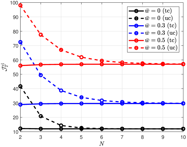
In order to show the influence of the different functions δi\delta_{i} on the transient performance bounds (22) and (26), we consider the worst-case disturbance sequence (w⁡(t)=w¯​∀t∈{0,…,T}w(t)=\bar{w}\ \forall t\in\{0,\dots,T\}) with different bounds w¯∈{0,0.3,0.5}\bar{w}\in\{0,0.3,0.5\} and compare the closed-loop transient performances of the real state sequence 𝒥Tcl​(x,N)\mathcal{J}^{\mathrm{cl}}_{T}(x,N) for the ”uc” case and the ”tc” case. Therefore, similar to the approach in Grüne and Panin 2015, we first fix T=20T=20 and set N=2,…,10N=2,\dots,10. The results can be found in Fig. 1, where the solid lines correspond to 𝒥Tcl,tc​(x,N)\mathcal{J}^{\mathrm{cl,tc}}_{T}(x,N) and dashed lines to 𝒥Tcl,uc​(x,N)\mathcal{J}^{\mathrm{cl,uc}}_{T}(x,N). The black lines restore the nominal (undisturbed) case. The closed-loop transient performance is almost the same for all prediction horizons NN when using terminal conditions, i.e. the function δ1​(N)\delta_{1}(N) has only little influence even for small NN. When omiting terminal conditions, the performance only converges to the ”tc” case with a larger NN. This difference can be explained by the fact that in the ”uc” case the closed-loop states only converge to a neighborhood of the ROSS (even without disturbances) and therefore the influence of δ3​(N)\delta_{3}(N) dominates for small NN (recall that δ3​(N)=δ1​(N)+ϵ1​(N)\delta_{3}(N)=\delta_{1}(N)+\epsilon_{1}(N)). A similar behavior can be observed in the disturbed cases with the difference that the performance declines for larger disturbances. This is to be expected and can be explained by the term T​κLπ​maxϵ∈Ω​‖ϵ‖T\kappa_{L_{\pi}}\max_{\epsilon\in\Omega}\|\epsilon\| in Corollaries 4.9 and 5.14, which increases with increasing w¯\bar{w}, but is independent of NN.

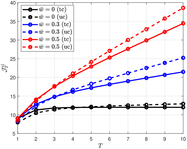
Fig. 2 shows the results for a fixed N=4N=4 and T=1,…,10T=1,\dots,10. Again, for w¯=0\bar{w}=0 the undisturbed case restores the results from Grüne and Panin 2015. In the ”uc” case the term T​δ3​(N)T\delta_{3}(N) in Corollary 5.14 reduces the performance for increasing TT while for the ”tc” case the performance converges to a constant (for OPENw¯=0)\bar{w}=0). With disturbances (w¯≠0\bar{w}\neq 0) the performances 𝒥Tcl,tc​(x,N)\mathcal{J}^{\mathrm{cl,tc}}_{T}(x,N) and 𝒥Tcl,uc​(x,N)\mathcal{J}^{\mathrm{cl,uc}}_{T}(x,N) both increase with increasing TT. This can be explained by the term T​κLπ​maxϵ∈Ω​‖ϵ‖T\kappa_{L_{\pi}}\max_{\epsilon\in\Omega}\|\epsilon\| in (22) and (26), which yields a steeper slope of the transient performances for larger disturbances.
Refer to caption
Figure 1: Closed-loop transient performances for T=20T=20, N=2,…,10N=2,\dots,10 and different disturbance bounds (worst-case disturbance sequence)
Refer to caption
Figure 2: Closed-loop transient performances for N=4N=4 and T=1,…,10T=1,\dots,10 and different disturbance bounds (worst-case disturbance sequence)

7 CONCLUSION

In this paper, we provided estimates for the closed-loop non-averaged and transient performance of robust economic MPC schemes. In presence of terminal conditions, it was shown that the closed-loop infinite horizon non-averaged performance of the nominal state sequence is approximately equal to the infinite-horizon optimal performance. For the case without terminal conditions, a similar performance estimate was stated on a finite horizon. Moreover, for both cases it was shown that the input sequences computed by the robust EMPC scheme yield, up to an error term, the optimal closed-loop transient performance among all input sequences which drive the nominal state to a neighborhood of the robust optimal steady state. The given results are similar to those of the nominal economic MPC case; the main difference and novelty in the derivation of the bounds in this work is that they hold for closed-loop nominal state sequences, which by the nature of the tube-based MPC scheme do not necessarily satisfy the nominal system dynamics. In addition, the performance estimates could be extended such that upper bounds for the closed-loop performance of the real (disturbed) state could also be provided.

References

  • Amrit et al. (2011) Amrit, R., Rawlings, J.B., and Angeli, D. (2011). Economic optimization using model predictive control with a terminal cost. Annual Reviews in Control, 35(2), 178–186.
  • Bayer (2017) Bayer, F. (2017). Performance and constraint satisfaction in robust economic model predictive control. Logos Verlag Berlin GmbH.
  • Bayer et al. (2014) Bayer, F.A., Müller, M.A., and Allgöwer, F. (2014). Tube-based robust economic model predictive control. Journal of Process Control, 24(8), 1237–1246.
  • Bayer et al. (2016) Bayer, F.A., Müller, M.A., and Allgöwer, F. (2016). Min-max economic model predictive control approaches with guaranteed performance. In 2016 IEEE 55th Conference on Decision and Control (CDC), 3210–3215.
  • Bayer et al. (2018) Bayer, F.A., Müller, M.A., and Allgöwer, F. (2018). On optimal system operation in robust economic MPC. Automatica, 88, 98–106.
  • Broomhead et al. (2015) Broomhead, T.J., Manzie, C., Shekhar, R.C., and Hield, P. (2015). Robust periodic economic MPC for linear systems. Automatica, 60, 30–37.
  • Dong and Angeli (2018) Dong, Z. and Angeli, D. (2018). Tube-based robust economic model predictive control on dissipative systems with generalized optimal regimes of operation. In 2018 IEEE Conference on Decision and Control (CDC), 4309–4314.
  • Faulwasser et al. (2018) Faulwasser, T., Grüne, L., and Müller, M.A. (2018). Economic nonlinear model predictive control. Foundations and Trends® in Systems and Control, 5(1), 224–409.
  • Grüne (2013) Grüne, L. (2013). Economic receding horizon control without terminal constraints. Automatica, 49(3), 725–734.
  • Grüne (2016) Grüne, L. (2016). Approximation properties of receding horizon optimal control. Jahresbericht der Deutschen Mathematiker-Vereinigung, 118(1), 3–37.
  • Grüne and Panin (2015) Grüne, L. and Panin, A. (2015). On non-averaged performance of economic MPC with terminal conditions. In 2015 54th IEEE Conference on Decision and Control (CDC), 4332–4337.
  • Grüne and Stieler (2014) Grüne, L. and Stieler, M. (2014). Asymptotic stability and transient optimality of economic MPC without terminal conditions. Journal of Process Control, 24(8), 1187–1196.
  • Lucia et al. (2014) Lucia, S., Andersson, J.A., Brandt, H., Diehl, M., and Engell, S. (2014). Handling uncertainty in economic nonlinear model predictive control: A comparative case study. Journal of Process Control, 24(8), 1247–1259.
  • Mayne et al. (2005) Mayne, D., Seron, M., and Raković, S. (2005). Robust model predictive control of constrained linear systems with bounded disturbances. Automatica, 41(2), 219–224.
  • Schwenkel et al. (2020) Schwenkel, L., Köhler, J., Müller, M.A., and Allgöwer, F. (2020). Robust economic model predictive control without terminal conditions. In 21st IFAC World Congress 2020.
  • Sontag (2013) Sontag, E.D. (2013). Mathematical Control Theory. Springer New York.