Buffered Streaming Graph Partitioning
Abstract.
Partitioning graphs into blocks of roughly equal size is a widely used tool when processing large graphs. Currently there is a gap observed in the space of available partitioning algorithms. On the one hand, there are streaming algorithms that have been adopted to partition massive graph data on small machines. In the streaming model, vertices arrive one at a time including their neighborhood and then have to be assigned directly to a block. These algorithms can partition huge graphs quickly with little memory, but they produce partitions with low solution quality. On the other hand, there are offline (shared-memory) multilevel algorithms that produce partitions with high quality but also need a machine with enough memory to partition huge networks. In this work, we make a first step to close this gap by presenting an algorithm that computes significantly improved partitions of huge graphs using a single machine with little memory in streaming setting. First, we adopt the buffered streaming model which is a more reasonable approach in practice. In this model, a processing element can store a buffer, or batch, of nodes (including their neighborhood) before making assignment decisions. When our algorithm receives a batch of nodes, we build a model graph that represents the nodes of the batch and the already present partition structure. This model enables us to apply multilevel algorithms and in turn compute much higher quality solutions of huge graphs on cheap machines than previously possible. To partition the model, we develop a multilevel algorithm that optimizes an objective function that has previously shown to be effective for the streaming setting. Surprisingly, this also removes the dependency on the number of blocks from the running time compared to the previous state-of-the-art. Overall, our algorithm computes, on average, better solutions than Fennel using a very small buffer size. In addition, for large values of our algorithm becomes faster than Fennel.
1. Introduction
Complex graphs are increasingly being used to model phenomena such as social networks, data dependency in applications, citations of papers, and biological systems like the human brain. Often these graphs are composed of billions of entities that give rise to specific properties and structures. As a concrete example to cope with such graphs, graph databases (Demirci et al. 2019) and graph processing frameworks (Ching et al. 2015; Malewicz et al. 2010; Gonzalez et al. 2012) can be used to store a graph, query it, and provide other operations. If the graphs become too large, then they have to be distributed over many machines in order for the system to provide scalable operations. A key operation for scalable computations on huge graphs is to partition its components among processing elements (PEs) such that each PE receives roughly the same amount of components and the communication between PEs in the underlying application is minimized. In the distributed setup, each PE operates on some portion of the graph and communicates with other PEs through message-passing. This operation is naturally modeled by the graph partitioning problem, which computes a partition of the graph into blocks such that the blocks have roughly the same size and the number of edges crossing blocks, i. e., communication, is minimized. Graph partitioning is NP-complete (Garey et al. 1974) and there can be no approximation algorithm with a constant ratio factor for general graphs (Bui and Jones 1992). Thus, heuristic algorithms are used in practice.
There has been an extensive body of work in the area of graph partitioning. Roughly speaking, there are streaming algorithms, internal memory (shared-memory parallel) algorithms and distributed memory parallel algorithms. However, currently there is a gap observed in the design space of available partitioning algorithms. First of all, the most popular streaming approach in literature is the one-pass model, in which vertices arrive one at a time including their neighborhood and then have to be permanently assigned to blocks. Algorithms based on this model can partition huge graphs quickly with little memory, but compute rather low-quality partitions. To improve partition quality, the graph can be restreamed while the one-pass algorithm updates block assignment, but this is still far behind offline approaches. Offline multilevel algorithms such as KaHIP (Sanders and Schulz 2011) or Metis (Karypis and Kumar 1998) are widely known and can produce partitions with high quality. Nevertheless they cannot partition huge graphs unless a machine with sufficient memory is used and hence can not be used for example for preprocessing in out-of-core algorithms. Lastly, distributed algorithms are able to partition huge graphs successfully and compute high-quality solutions. However, they require a large amount of computational resources and typically access to a supercomputer, which can be infeasible depending on the application. Moreover, a distributed partitioning algorithm needs to split the input graph among different machines before actually partitioning it. When the graph is too large, this preliminary partition has to be generated on the fly by a stream partitioning algorithm while loading the graph. Other natural applications for stream partitioning include distributed graph processing systems based on a load-compute-store logic such as MapReduce (Dean and Ghemawat 2008) and Giraph (Ching et al. 2015), and systems which support native graph-as-a-stream computations such as Kineograph (Cheng et al. 2012), and Apache Flink (Carbone et al. 2015).
Contribution. In this work, we start to fill the gap currently observed for the existing graph partitioning algorithms. We propose an algorithm that can compute significantly better partitions of huge graphs than the currently available streaming algorithms while using a single machine without a lot of memory. We adopt the buffered streaming model which allows a buffer of nodes to be received and stored before making assignment decisions. Our algorithm is carefully engineered to produce partitions of improved quality by using a sophisticated multilevel scheme on a compressed model of the buffer and the already assigned vertices. Our multilevel algorithm optimizes for the same objective as the previous state-of-the-art Fennel. However, due to the multilevel scheme used on the compressed model, our local search algorithms have a global view on the optimization problem and hence compute better solutions overall. Lastly, using the multilevel scheme reduces the time complexity from of Fennel to , where is the number of blocks a graph has to be partitioned in. To this end, experiments indicate that our algorithm can partition huge networks on machines with small memory while computing better solutions than the previous state-of-the-art in the streaming setting. At the same time our algorithm is faster than the previous state-of-the-art for larger values of blocks .
2. Preliminaries
2.1. Basic Concepts
Let be an undirected graph with no multiple or self edges allowed, such that and . Let be a node-weight function, and let be an edge-weight function. We generalize and functions to sets, such that and . Let denote the neighbors of . A graph is said to be a subgraph of if and . When , is an induced subgraph. Let be the degree of node , be the maximum degree of , and be the maximum degree of the subgraph induced by . The graph partitioning problem (GP) consists of assigning each node of to exactly one of distinct blocks respecting a balancing constraint in order to minimize the edge-cut. More precisely, GPP partitions into blocks ,…, (i. e., and for ), which is called a -partition of . The balancing constraint demands that the sum of node weights in each block does not exceed a threshold associated with some allowed imbalance . More specifically, .
The edge-cut of a -partition consists of the total weight of the edges crossing blocks, i. e., , where . An abstract view of the partitioned graph is a quotient graph , in which nodes represent blocks and edges are induced by the connectivity between blocks. More precisely, each node of has weight and there is an edge between and if there is at least one edge in the original partitioned graph that runs between the blocks and . We call neighboring blocks a pair of blocks that is connected by an edge in the quotient graph. A vertex that has a neighbor , is a boundary vertex. A successful heuristic for partitioning large graphs is the multilevel graph partitioning (MGP) approach depicted in Figure 1, where the graph is recursively contracted to achieve smaller graphs which should reflect the same basic structure as the input graph. After applying an initial partitioning algorithm to the smallest graph, the contraction is undone and, at each level, a local search method is used to improve the partitioning induced by the coarser level. Contracting a cluster of nodes consists of replacing these nodes by a new node . The weight of this node is set to the sum of the weight of the cluster vertices. Moreover, the new node is connected to all elements , . This ensures that a partition from a coarser level that is transfered to a finer level maintains the edge cut and the balance of the partition. The uncontraction of a node undoes the contraction. Local search moves vertices between the blocks in order to reduce the objective.
Computational Models. The focus of this paper is to engineer a graph partitioning algorithm for a streaming input. In particular, the input is a stream of nodes alongside with their respective adjacency lists. The classic streaming model is the one-pass model, in which the nodes have to be permanently assigned to a block as soon as they are loaded from the input. As soon as assignment decisions of an algorithm for the current node depend on the previous decisions, an algorithm in the model has to store the assignment of the previous loaded nodes and hence needs space. We use an extended version of this model, which is called the buffered streaming model. More precisely, a -sized buffer or batch of input nodes with their neighborhood is repeatedly loaded. Partition/block assignment decisions have to be made after the whole buffer is loaded. While we investigate the dependence of our algorithm on this parameter, in practice the parameter will depend on the amount of available memory on a machine. The parameter can be dynamically chosen such that the buffer is “full” if space has been loaded from the disk. Hence the buffered streaming model asymptotically does not need more space than a one-pass streaming algorithm if this setting is used. This holds true even in the worst case: when a node has degree close to . In this paper, we use a constant throughout the run of an algorithm. For a predefined batch size , the total amount of batches are consecutively loaded and assigned to blocks.
2.2. Related Work
There has been a large amount of research on graph partitioning. We refer the reader to (Bichot and Siarry 2011; Buluç et al. 2016; Schulz and Strash 2019) for extensive material and references. Here, we focus on results close to our main contribution. The most successful general-purpose offline algorithms to solve the graph partitioning problem for huge real-world graphs are based on the multilevel approach. The most commonly used formulation of the multilevel scheme for graph partitioning was proposed in (Hendrickson and Leland 1995). However, these algorithms require the graph to fit into main memory of a single machine or into the memory of a distributed machine if a distributed memory parallel partitioning algorithm is used.
Stanton and Kliot (Stanton and Kliot 2012) introduced graph partitioning in the streaming model and proposed many natural heuristics to solve it. These heuristics include one-pass methods such as Hashing, Chunking, and linear deterministic greedy (LDG), and some buffered methods such as greedy evocut. The evocut buffered model is different from our model as it is an extended one-pass model in which a buffer of fixed size is kept and the algorithm can assign any node from the buffer to a block, rather than the one that has been received most recently. However, all methods that use a buffer perform significantly worse than random partitionings – hence we do not include them in our experiments. In their experiments, LDG had the best overall results in terms of total edge-cut. In this algorithm, node assignments prioritize blocks containing more neighbors while using a penalty multiplier to control imbalance. In particular, it assigns a node to the block that maximizes with being a multiplicative penalty defined as . The intuition here is that the penalty avoids to overload blocks that are already very heavy. Tsourakakis et al. (Tsourakakis et al. 2014) proposed a one-pass partitioning heuristic named Fennel, which is an adaptation of the widely-known clustering objective modularity (Brandes et al. 2007). Roughly speaking, Fennel assigns a node to a block , respecting a balancing threshold, in order to maximize an expression of type , i. e., with an additive penalty. The assignment decision of Fennel is based on an interpolation of two properties: attraction to blocks with more neighbors and repulsion from blocks with more non-neighbors. When is a constant, the resulting objective function coincides with the first property. If , the objective function coincides with the second property. More specifically, the authors defined the Fennel objective function by using , in which is a free parameter and . After a parameter tuning made by the authors, Fennel uses , which provides . Note that in the original paper, the authors assume to be constant and hence derive a complexity of . However, since one has to iterate over all blocks for each node the complexity of the algorithm depends on and is given by .
A restreaming approach has been introduced by Nishimura and Ugander (Nishimura and Ugander 2013). In this model, multiple passes through the entire input are allowed, to allow iterative improvements. The authors proposed easily implementable restreaming versions of LDG and Fennel: ReLDG and ReFennel. Awadelkarim and Ugander (Awadelkarim and Ugander 2020) studied the effect of node ordering for streaming graph partitioning. The authors introduced the notion of prioritized streaming, in which (re)streamed nodes are statically or dynamically reordered based on some priority. Patwary et al. (Patwary et al. 2019) proposed WStream, a greedy stream graph partitioning algorithm that keeps a sliding stream window. This sliding window contains a few hundred nodes such that it gives more information about the next node to be allocated to a block. However, the code is not available and the algorithm has only been evaluated on graphs with a few thousand vertices. Jafari et al. (Jafari et al. 2021) proposed a shared-memory partitioning algorithm based on a buffered streaming computational model similar to the one we use here. Their algorithm uses the idea of multilevel algorithm but with a simplified structure in which the LDG one-pass algorithm constitutes the coarsening step, the initial partitioning, and the local search during uncoarsening. Our work differs from theirs in the fact that we focus on single-threaded execution, we construct a sophisticated model instead of processing the nodes of a batch directly, and our algorithm is inspired on the Fennel one-pass algorithm, which outperformed LDG in previously published studies. There are also a wide range of algorithms that focus on (buffered) streaming edge partitioning (Petroni et al. 2015; Mayer et al. 2018; Sajjad et al. 2016). However, as our focus is on edge cut-based algorithms they are beyond the scope of this work.
3. Buffered Graph Partitioning
We now present our main contribution, namely HeiStream: a novel algorithm to solve graph partitioning in the buffered streaming model. We start by first outlining the overall structure behind HeiStream and then we present each of the algorithm components.
3.1. Overall Structure
We now explain the overall structure of HeiStream. We slide through the streamed graph by repeating the following successive operations until all the nodes of are assigned to blocks. First, we load a batch containing nodes alongside with their adjacency lists. Second, we build a model to be partitioned. This model represents the already partitioned vertices as well as the nodes of the current batch. Third, we partition with a multilevel partitioning algorithm to optimize for the Fennel objective function. And finally, we permanently assign the nodes from the current batch to blocks. Algorithm 1 summarizes the general structure of HeiStream and Figure 2 shows the detailed structure of HeiStream.
3.2. Model Construction
We build two different models, which yield a running time–quality trade-off. We start by describing the basic model and then extend this later. When a batch is loaded, we build the model as follows. We initialize as the subgraph of induced by the nodes of the current batch. If the current batch is not the first one, we add artificial nodes to the model. These represent the preliminary blocks in their current state, i.e., filled with the nodes from the previous batches, which were already assigned. The weight of an artificial node is set to the weight of block . A node of the current batch is connected to an artificial node if it has a neighbor from the previous batch that has been assigned to block . If this creates parallel edges, we replace them by a single edge with its weight set to the sum of the weight of the parallel edges. Note that the basic model does ignore edges towards nodes that will be streamed in future batches, i. e., batches that have not been streamed yet. Our extended model incorporates edges towards nodes from future, not yet loaded, batches – if the stream contains such edges. We call edges towards nodes of future batches ghost edges and the corresponding endpoint in the future batch ghost node. Ghost nodes and ghost edges provide partial information about parts of that have not yet been streamed. Hence, representing them in the model enhances the partitioning process. Note though that simply inserting all ghost nodes and edges can overload memory in case there is an excessive amount of them. Thus our approach consists of randomly contracting the ghost nodes with one of their neighboring nodes from the current batch. Note that this contraction increments the weight of a node within our model and ensures that if there are more than one node from the current batch connected to the same future node, then there will be edges between those nodes in our model. Also note that the contraction ensures that the number of nodes in all models throughout the batched streaming process is constant. This prevents memory from being overloaded and makes it unnecessary to reallocate memory for between successive batches. In order to give a lower priority to ghost edges in comparison to the other edges, we divide the weight of each ghost edge by 2 in our model. The construction of the extended model is conceptually illustrated in Figure 2.
3.3. Multilevel Weighted Fennel
Our approach to partition the model is a multilevel version of the algorithm Fennel. Recall that the multilevel scheme consists of three successive phases: coarsening, initial partitioning, and uncoarsening, as depicted in Figure 1. Note, however, that the artificial nodes in our model can become very heavy and are not allowed to be contracted or change their block. As a consequence, these nodes need special handling in our multilevel algorithm. Moreover, the Fennel algorithm is designed for unweighted graphs, hence it needs some adaptation to be used in HeiStream. We introduce a generalization of Fennel for weighted graphs that can be directly employed in a multilevel algorithm. In this section, we present this generalized Fennel objective and explain the details of our multilevel algorithm to partition the model.
3.3.1. Generalized Fennel.
As already mentioned, adaptations are necessary to implement Fennel for weighted graphs, in particular in a multilevel scheme. First, note that the original formulation of Fennel only works for unweighted graphs (Tsourakakis et al. 2014). However, our model has nodes and edges that are weighted – due to connections to the artificial nodes as well as future nodes that may be contracted into the model. Moreover, the multilevel scheme creates a sequence of weighted graphs. Note that a generalization of the Fennel gain function has to ensure that the gain of a node on a coarser level corresponds to the sum of the gains of the nodes that it represents on the finest level. This way the algorithm gets a global view onto the optimization problem on the coarser levels and a very local view on the finer levels. Moreover, it is ensured that on each level of the hierarchy the algorithm works towards optimizing the given objective.
Our generalization of the gain function of Fennel is as follows. Let be the node that should be assigned to a block to another block. Our generalized Fennel assigns to a block that maximizes , such that . Note that this is a direct generalization of the unweighted case. First, if the graph does not have edge weights, then the first part of the equation becomes which is the first part of the Fennel objective. Second, if the graph also does not have node weights, then the second part of the equation is the same as the second part of the equation in the Fennel objective. Moreover, observe that the penalty term in our objective is multiplied by . This is done to have the property stated above and formalized in Theorem 3.1. Finally, we keep the original value of the parameters and in order to keep consistency.
Theorem 3.1.
If a set of nodes is contracted into a node , the generalized Fennel gain function of is equal to the sum of the generalized Fennel gain functions of the nodes in .
Proof.
On the one hand, the generalized Fennel gain of assigning a node to a block is . On the other hand, the sum of the generalized Fennel gains of assigning all nodes in to a block can be expressed as . Since the factor is identical in both expressions, the two of them are equivalent if the following equalities hold: and . Both of these equalities are trivially true as a property of the contraction process. ∎
3.3.2. Multilevel Fennel.
We now explain our multilevel algorithm to partition the model . Our coarsening phase is an adapted version of the size-constraint label propagation approach (Meyerhenke et al. 2014). To be self-contained, we shortly outline the coarsening approach and then show how to modify it to be able to handle artificial nodes. To compute a graph hierarchy, the algorithm computes a size-constrained clustering on each level and contract that to obtain the next level. The clustering is contracted by replacing each cluster by a single node, and the process is repeated recursively until the graph becomes small enough. This hierarchy is then used by the algorithm. Due to the way we define contraction, it ensures that a partition of a coarse graph corresponds to a partition of all the finer graphs in the hierarchy with the same edge-cut and balance. Note that cluster contraction is an aggressive coarsening strategy. In contrast to matching-based approaches, it enables us to drastically shrink the size of irregular networks. The intuition behind this technique is that a clustering of the graph (one hopes) contains many edges running inside the clusters and only a few edges running between clusters, which is favorable for the edge cut objective.
The algorithm to compute clusters is based on label propagation (Raghavan et al. 2007) and avoids large clusters by using a size constraint, as described in (Meyerhenke et al. 2014). For a graph with nodes and edges, one round of size-constrained label propagation can be implemented to run in time. Initially, each node is in its own cluster/block, i. e., the initial block ID of a node is set to its node ID. The algorithm then works in rounds. In each round, all the nodes of the graph are traversed. When a node is visited, it is moved to the block that has the strongest connection to , i. e., it is moved to the cluster that maximizes . Ties are broken randomly. We perform at most rounds, where is a tuning parameter.
In HeiStream, we have to ensure that two artificial nodes are not contracted together since each of them should remain in its previously assigned block. We achieve this by ignoring artificial nodes and artificial edges during the label propagation, i. e., artificial nodes cannot not change their label and nodes from the batch can not change their label to become a label of an artificial node. As a consequence, artificial nodes are not contracted during coarsening. Overall, we repeat the process of computing a size-constrained clustering and contracting it, recursively. As soon as the graph is small enough, i. e., it has fewer nodes than an threshold, it is initially partitioned by an initial partitioning algorithm. More precisely, we use the threshold , in which is a tuning parameter. Note that, for large enough buffer sizes, this threshold will be .
When the coarsening phase ends, we run an initial partitioning algorithm to compute an initial -partition for the coarsest version of . That means that all nodes other than the artificial nodes, which are already assigned, will be assigned to blocks. To assign the nodes, we run our generalized Fennel algorithm with explicit balancing constraint , i. e., the weight of no block will exceed . To be precise, a node will be assigned to a block that maximizes , such that and . Note that the algorithm at this point considers all possible blocks and hence has complexity proportional to . However, as the coarsest graph has nodes, overall the initial partitioning needs time which is linear in the size of the input model. When initial partitioning is done, we transfer the current solution to the next finer level by assigning each node of the finer level to the block of its coarse representative. At each level of the hierarchy, we apply a local search algorithm. Our local search algorithm is the same size-constraint label propagation algorithm we used in the contraction phase but with a different objective function. Namely, when visiting a node node, we remove it from its current block and then we assign it to the neighboring block which maximizes the generalized Fennel gain function defined above. Note that, in contrast to the initial partitioning, only blocks of adjacent nodes are considered here. Hence, one round of the algorithm can still be implemented to run in linear time in the size the current level. As in the coarsening phase, artificial nodes cannot be moved between blocks. Differently though, we do not exclude the artificial nodes from the label propagation here. This is the case because the artificial nodes and their edges are used to compute the generalized Fennel gain function of the other nodes. As in the initial partitioning, we use the explicit size constraint of . As a side note, we also tried to use high-quality offline algorithms as initial partitioning algorithms, however, in preliminary experiments this results in very unbalanced blocks (even with adaptively configured balance constraints) and overall in reduced quality throughout the process. Hence, we did not consider this further.
Assuming geometrically shrinking graphs thoughout the hierarchy and assuming that the buffer size is larger than the number of blocks , then the overall running time to partition a batch is linear in the size of the batch. This is due to the fact that the overall running time of coarsening and local search sums up to be linear in the size of the batch, while the overall running time of the initial partitioning depends linearly on the size of the input model. Summing this up over all batches yields overall linear running time .
3.4. Restreaming
We now extend HeiStream to operate in a restreaming setting. During restreaming, the overall structure of the algorithm is roughly the same. Nevertheless we need to implement some adaptations which we explain in this section. The first adaptations concern model construction. Recall that the nodes from the current batch are already assigned to blocks during the previous pass of the input. We explicitly assign these nodes to their respective blocks in . Furthermore, ghost nodes and edges are not needed to construct . This is the case since all nodes from future batches are already known and assigned to blocks, i. e., these nodes will be represented in the artificial nodes. More precisely, we adapt the artificial nodes to represent the nodes from all batches except the current one. Since a partition of the graph is already given, we do not allow the contraction of cut edges during restreaming in the coarsening phase of our multilevel scheme. That means that clusters are only allowed to grow inside blocks. As a consequence, we can directly use the partition computed in the previous pass as initial partitioning for so we do not need to run an initial partitioning algorithm.
3.5. Implementation Details
Our implementation of is based on an adjacency array and consecutive node IDs. We reserve the first IDs for the nodes from the current batch, which keep their global order. This means that, when we process the batch, nodes IDs can be easily converted from our model to and the other way around by respectively summing or subtracting on their ID. Similarly, we reserve the last IDs of for the artificial nodes and keep their relative order for all batches. Note that this configuration separates mutable nodes (nodes from current batch) and immutable nodes (artificial nodes). This allows us to efficiently control which nodes are allowed to move during coarsening, initial partitioning, and local search. We keep an array of size store the permanent block assignment of the nodes of . To improve running time, we use approximate computation of powering in our Fennel function.
4. Experimental Evaluation
| Graph | Type | ||
| Tuning Set | |||
| coAuthorsCiteseer | 227 320 | 814 134 | Citations |
| citationCiteseer | 268 495 | 1 156 647 | Citations |
| amazon0312 | 400 727 | 2 349 869 | Co-Purch. |
| amazon0601 | 403 364 | 2 443 311 | Co-Purch. |
| amazon0505 | 410 236 | 2 439 437 | Co-Purch. |
| roadNet-PA | 1 087 562 | 1 541 514 | Roads |
| com-Youtube | 1 134 890 | 2 987 624 | Social |
| soc-lastfm | 1 191 805 | 4 519 330 | Social |
| roadNet-TX | 1 351 137 | 1 879 201 | Roads |
| in-2004 | 1 382 908 | 13 591 473 | Web |
| G3_circuit | 1 585 478 | 3 037 674 | Circuit |
| soc-pokec | 1 632 803 | 22 301 964 | Social |
| as-Skitter | 1 694 616 | 11 094 209 | Aut.Syst. |
| wiki-topcats | 1 791 489 | 28 511 807 | Social |
| roadNet-CA | 1 957 027 | 2 760 388 | Roads |
| wiki-Talk | 2 388 953 | 4 656 682 | Web |
| soc-flixster | 2 523 386 | 7 918 801 | Social |
| del22 | 4 194 304 | 12 582 869 | Artificial |
| rgg22 | 4 194 304 | 30 359 198 | Artificial |
| del23 | 8 388 608 | 25 165 784 | Artificial |
| rgg23 | 8 388 608 | 63 501 393 | Artificial |
| Huge Graphs | |||
| uk-2005 | 39 459 923 | 783 027 125 | Web |
| twitter7 | 41 652 230 | 1 202 513 046 | Social |
| sk-2005 | 50 636 154 | 1 810 063 330 | Web |
| soc-friendster | 65 608 366 | 1 806 067 135 | Social |
| er-fact1.5s26 | 67 108 864 | 907 090 182 | Artificial |
| RHG1 | 100 000 000 | 1 000 913 106 | Artificial |
| RHG2 | 100 000 000 | 1 999 544 833 | Artificial |
| uk-2007-05 | 105 896 555 | 3 301 876 564 | Web |
| Graph | Type | ||
|---|---|---|---|
| Test Set | |||
| Dubcova1 | 16 129 | 118 440 | Meshes |
| hcircuit | 105 676 | 203 734 | Circuit |
| coAuthorsDBLP | 299 067 | 977 676 | Citations |
| Web-NotreDame | 325 729 | 1 090 108 | Web |
| Dblp-2010 | 326 186 | 807 700 | Citations |
| ML_Laplace | 377 002 | 13 656 485 | Meshes |
| coPapersCiteseer | 434 102 | 16 036 720 | Citations |
| coPapersDBLP | 540 486 | 15 245 729 | Citations |
| Amazon-2008 | 735 323 | 3 523 472 | Similarity |
| eu-2005 | 862 664 | 16 138 468 | Web |
| web-Google | 916 428 | 4 322 051 | Web |
| ca-hollywood-2009 | 1 087 562 | 1 541 514 | Roads |
| Flan_1565 | 1 564 794 | 57 920 625 | Meshes |
| Ljournal-2008 | 1 957 027 | 2 760 388 | Social |
| HV15R | 2 017 169 | 162 357 569 | Meshes |
| Bump_2911 | 2 911 419 | 62 409 240 | Meshes |
| del21 | 2 097 152 | 6 291 408 | Artificial |
| rgg21 | 2 097 152 | 14 487 995 | Artificial |
| FullChip | 2 987 012 | 11 817 567 | Circuit |
| soc-orkut-dir | 3 072 441 | 117 185 083 | Social |
| patents | 3 750 822 | 14 970 766 | Citations |
| cit-Patents | 3 774 768 | 16 518 947 | Citations |
| soc-LiveJournal1 | 4 847 571 | 42 851 237 | Social |
| circuit5M | 5 558 326 | 26 983 926 | Circuit |
| italy-osm | 6 686 493 | 7 013 978 | Roads |
| great-britain-osm | 7 733 822 | 8 156 517 | Roads |
Methodology. We performed the implementation of HeiStream and competing algorithms inside the KaHIP framework (using C++) and compiled them using gcc 9.3 with full optimization turned on (-O3 flag). Since no official versions of the one-pass streaming and restreaming algorithms are available in public repositories, we implemented them in our framework. Our implementations of these algorithms reproduce the results presented in the respective papers and are optimized for running time as much as possible. To this end, we implemented Hashing, LDG, Fennel, and ReFennel. Multilevel LDG (Jafari et al. 2021) is also not publicly available. We sent a message to the authors requesting an executable version of their algorithm for our tests but we have not receive any response up to the moment this work was submitted. Hence, we compare HeiStream against Multilevel LDG based on the results explicitly reported in (Jafari et al. 2021). We have used two machines. Machine A has a two six-core Intel Xeon E5-2630 processor running at GHz, GB of main memory, and MB of L2-Cache. It runs Ubuntu GNU/Linux 20.04.1 and Linux kernel version 5.4.0-48. Machine B has a four-core Intel Xeon E5420 processor running at GHz, GB of main memory, and MB of L2-Cache. The machine runs Ubuntu GNU/Linux 20.04.1 and Linux kernel version 5.4.0-65. Most of our experiments were run on a single core of Machine A. The only exceptions are the experiments with huge graphs, which were run on a single core of Machine B. When using machine A, we stream the input directly from the internal memory, and when using machine , that only has 16GB of main memory, we stream the input from the hard disk.
We use for most experiments. We allow an imbalance of for all experiments (and all algorithms). All partitions computed by all algorithms have been balanced. Depending on the focus of the experiment, we measure running time and/or edge-cut. In general, we perform ten repetitions per algorithm and instance using different random seeds for initialization, and we compute the arithmetic average of the computed objective functions and running time per instance. When further averaging over multiple instances, we use the geometric mean in order to give every instance the same influence on the final score. Unless explicitly mentioned otherwise, we average all results of each algorithm grouped by . For a -partition generated by an algorithm , we express its score (which can be edge-cut or running time) using one or more of the following tools: improvement over an algorithm , computed as ; ratio, computed as with being the maximum score for among all competitors including ; relative value over an algorithm , computed as . We also present performance profiles which relate the running time (resp. solution quality) of a group of algorithms to the fastest (resp. best) one on a per-instance basis (rather than grouped by ). Their x-axis shows a factor while their y-axis shows the percentage of instances for which A has up to times the running time (resp. solution quality) of the fastest (resp. best) algorithm.
Instances. We get graphs from various sources to test our algorithm (Leskovec and Krevl 2014; Rossi and Ahmed 2015; Bader et al. 2014; Holtgrewe et al. 2010; Funke et al. 2019). Most of the considered graphs were used for benchmark in previous works on graph partitioning. The graphs wiki-Talk and web-Google, as well as most networks of co-purchasing, roads, social, web, autonomous systems, citations, circuits, similarity, meshes, and miscellaneous are publicly available either in (Leskovec and Krevl 2014) or in (Rossi and Ahmed 2015). Prior to our experiments, we converted these graphs to a vertex-stream format while removing parallel edges, self loops, and directions, and assigning unitary weight to all nodes and edges. We also use graphs such as eu-2005, in-2004, uk-2002, and uk-2007-05, which are available at the 10th DIMACS Implementation Challenge website (Bader et al. 2014). Finally, we include some artificial random graphs. We use the name rggX for random geometric graph with nodes where nodes represent random points in the unit square and edges connect nodes whose Euclidean distance is below . We use the name delX for a graph based on a Delaunay triangulation of random points in the unit square (Holtgrewe et al. 2010). We use the name RHGX for random hyperbolic graphs (Funke et al. 2019; Penschuck et al. 2020) with nodes and edges. Basic properties of the graphs under consideration can be found in Table 1. For our experiments, we split the graphs in three disjoint sets. A tuning set for the parameter study experiments, a test set for the comparisons against the state-of-the-art, and a set of huge graphs for special larger scale tests. In any case, when streaming the graphs we use the natural given order of the nodes.
4.1. Parameter Study
We now present experiments to tune HeiStream and explore its behavior. We do this on the tuning set of our instance set. In our strategy, each experiment focuses on a single parameter of the algorithm while all the other ones are kept invariable. We start with a baseline configuration consisting of the following parameters: rounds in the coarsening label propagation, round in the local search label propagation, and in the expression of the coarsest model size. After each tuning experiment, we update the baseline to integrate the best found parameter. Unless explicitly mentioned otherwise, we run the experiments of this section over all tuning graphs from Table 1 based on the extended model construction, i. e., including ghost nodes and edges, for a buffer size of .
Tuning. We begin by evaluating how the number of label propagation rounds during local search affects running time and solution quality. In particular, we run configurations of HeiStream with , , and rounds and report results in Figures 3(a) and 3(b). Observe that the results of the baseline have considerably lower solution quality than the other ones overall. On the other hand, the results of the configurations with and rounds differ slightly to each other. On average, they respectively improve solution quality and over the baseline. Regarding running time, they respectively increase and on average over the baseline. Since the variation of quality for these two configurations is not significant, we decided to integrate the fastest one among them in the algorithm, namely the -round configuration.
Next we look at the parameter associated with the expression , which determines the size of the coarsest model. We run experiments for , with , and report results in Figure 3(c). We omit running time charts for this experiment since the tested configurations present comparable behavior in this regard. Figure 3(c) shows that the baseline presents the overall worst solution quality while and present the overall best solution quality. Averaging over all instances, these two latter configurations produce results respectively and better than the baseline. In light of that, we decide in favor of to compose HeiStream.
Exploration. We start the exploration of open parameters by investigating how the buffer size affects solution quality and running time. We use as baseline a buffer of nodes and successively double its capacity until any graph from the tuning set in Table 1 fits in a single buffer. We plot our results in Figures 4(b) and 4(c). Note that solution quality and running time increase regularly as the buffer size becomes larger. This behavior occurs because larger buffers enable more comprehensive and complex graph structures to be exploited by our multilevel algorithm. As a consequence, there is a trade-off between solution quality and resource consumption. In other words, we can improve partitioning quality at the cost of considerable extra memory and slightly more running time. Otherwise, we can save memory as much as possible and get a faster partitioning process at the cost of lowering solution quality. In practice, it means that HeiStream can be adjusted to produce partitions as refined as possible with the resources available in a specific system. For the extreme case of a single-node buffer, HeiStream behaves exactly as Fennel, while it behaves as an internal memory partitioning algorithm for the opposite extreme case.
Next, we compare the effect of using the extended model, which incorporates ghost nodes, over the basic model, which ignores ghost nodes. Figures 5(a) and 5(b) displays the results. The results show that the extended model provides improved quality over the basic model, with an improvement on average. This happens because the presence of ghost nodes and edges expands the perspective of the partitioning algorithm to future batches. This has a similar effect to increasing the size of the buffer, but at no considerable extra memory cost. Regarding running time, the results show that the extended model is consistently slower than the basic model for all values of . Averaging over all instances, the extended model costs more running time than the basic model. This increase in running time is explained by the higher number of edges to be processed when ghost nodes are incorporated in the model. As a practical conclusion from the experiment, the extended model can be used for better overall partitions with no significant extra memory but at the cost of extra running time. Otherwise, the basic model can be used for a consistently faster execution at the cost of a lower solution quality.
Finally, we test to what extent solution quality can be improved by restreaming HeiStream multiple times. We investigate this by restreaming each input graph times. We collect results after each pass and plot in Figure 4(a). The first restream generates a considerable quality jump, with an improvement over the baseline of on average. Each following pass has a positive impact on solution quality, which converges to be a -improvement on average over the baseline after the last pass. On the other hand, the running time has a roughly linear increase for each pass over the graph. In practice, this adds another degree of freedom to configure HeiStream for the needs of real systems.
4.2. Comparison against State-of-the-Art
| Cut Edges (%) | |||||||
| Graph | HS(Int.) | MLDG(Int.) | HS(32k) | -ReFennel | Fennel | LDG | Hashing |
| Dubcova1 | 13.68 | 14.26 | 13.68 | 29.19 | 33.99 | 33.96 | 95.62 |
| hcircuit | 2.73 | 17.75 | 2.53 | 21.86 | 28.97 | 28.97 | 90.75 |
| coAuthorsDBLP | 15.99 | 24.82 | 17.80 | 24.28 | 27.12 | 27.12 | 94.80 |
| Web-NotreDame | 5.85 | 11.01 | 9.20 | 12.58 | 19.52 | 19.56 | 95.97 |
| Dblp-2010 | 11.31 | 18.52 | 13.42 | 22.93 | 28.82 | 28.80 | 92.49 |
| ML_Laplace | 7.93 | 13.44 | 8.36 | 7.82 | 7.92 | 5.77 | 96.37 |
| coPapersCiteseer | 8.23 | 11.22 | 10.29 | 9.63 | 12.88 | 12.27 | 96.52 |
| coPapersDBLP | 14.51 | 19.29 | 18.33 | 16.47 | 20.65 | 20.22 | 96.39 |
| Amazon-2008 | 10.09 | 19.01 | 15.56 | 28.92 | 37.07 | 37.07 | 94.68 |
| eu-2005 | 11.14 | 14.57 | 18.64 | 25.53 | 35.88 | 31.96 | 96.44 |
| Web-Google | 1.62 | 9.66 | 9.48 | 18.04 | 30.64 | 30.64 | 96.87 |
| ca-hollywood-2009 | 35.34 | 32.51 | 42.36 | 41.34 | 44.54 | 45.25 | 96.62 |
| Flan_1565 | 7.69 | 9.36 | 8.12 | 10.26 | 10.59 | 6.70 | 96.61 |
| Ljournal-2008 | 29.12 | 34.76 | 38.58 | 43.23 | 51.43 | 51.36 | 96.07 |
| HV15R | 14.09 | 11.48 | 17.48 | 15.05 | 16.39 | 15.49 | 96.84 |
| Bump_2911 | 8.66 | 11.73 | 8.23 | 8.61 | 8.65 | 8.30 | 96.19 |
| FullChip | 38.20 | 48.16 | 45.71 | 57.39 | 61.93 | 64.23 | 95.06 |
| patents | 15.57 | 29.12 | 60.56 | 52.60 | 70.98 | 70.98 | 96.88 |
| Cit-Patents | 15.75 | 28.65 | 60.76 | 51.62 | 72.16 | 72.16 | 96.88 |
| Soc-LiveJournal1 | 29.72 | 35.69 | 35.62 | 34.00 | 39.03 | 45.62 | 96.66 |
| circuit5M | 40.02 | 34.60 | 41.00 | 75.45 | 78.42 | 78.47 | 96.87 |
| del21 | 1.38 | - | 8.53 | 33.52 | 40.21 | 40.21 | 93.39 |
| rgg21 | 1.53 | - | 1.52 | 4.09 | 5.02 | 4.88 | 96.89 |
| soc-orkut-dir | 37.86 | - | 54.76 | 47.22 | 55.85 | 60.27 | 96.85 |
| italy-osm | 0.13 | - | 1.34 | 4.65 | 4.80 | 4.80 | 78.11 |
| great-britain-osm | 0.16 | - | 1.63 | 7.18 | 7.34 | 7.34 | 79.94 |
In this section, we show experiments in which we compare HeiStream against the current state-of-the-art algorithms. Unless mentioned otherwise, these experiments involve all the graphs from the Test Set group in Table 1 and focus on two particular configurations of HeiStream, which we refer to as HeiStream(32k) and HeiStream(Int.). The first configuration is based on batches of size 32 768, while the second one has enough batch capacity to operate as an internal memory algorithm – both configurations perform a single pass over the input using the extended model.
Internal memory algorithms such as Metis (Karypis and Kumar 1998) and KaHIP (Sanders and Schulz 2011) are beyond the scope of this work since it is common knowledge that internal memory algorithms are better than streaming algorithms regarding partition quality if the instances fits in the memory of a machine. For the sake of reproducibility, we ran Metis and the fast social version of KaHIP over our Test Set group of instances for . On average, Fennel cuts a factor more edges than Metis and the fast social version of KaHIP, while HeiStream(Int.) cuts a factor more edges than both. Furthermore, Fennel is respectively a factor and a factor faster than Metis and the fast social version of KaHIP, while HeiStream(Int.) is slower than Metis and faster than the fast social version of KaHIP.
Results. We now present a detailed comparison of HeiStream (HS) against the state-of-the-art. In the results, we refer to the internal memory version of Multilevel LDG as MLDG(Int.). Moreover, we refer to the restreaming version of Fennel that passes over the graph times as -ReFennel. First, we focus on and later on choose a much wider range for the number of blocks. Table 2 shows the percentage of edges cut in the partitions generated by each algorithm for the graphs in the Test Set for . HeiStream(Int.) and HeiStream(32k) outperform all the other competitors for the majority of instances. First, both outperform Hashing for all graphs and LDG for out of the graphs. Next, both outperform Fennel in instances. The algorithm -ReFennel is outperformed by HeiStream(Int.) and HeiStream(32k) in and instances, respectively. Considering only the 21 instances for which there are results reported for Multi.LDG(Int.) in literature, the algorithms HeiStream(Int.) and HeiStream(32k) compute better partitions for and instances respectively.
For a closer comparison against Multi.LDG(Int.), we present Figure 6. We plot edge-cut values for Multi.LDG(Int.) based on results graphically reported in (Jafari et al. 2021). In this figure, we show of HeiStream(Int.) and HeiStream(32k) for particular graphs with . For all these instances, HeiStream(Int.) outperforms Multi.LDG(Int.) by a considerable margin. Observe that HeiStream(32k) outperforms the internal memory version of Multilevel LDG for the majority of instances. We omit additional comparisons against buffered versions of Multilevel LDG, since they provide lower quality than the internal memory version. We ran wider experiments over our whole Test Set for different values of . Figure 7 shows a quality improvement plot over Fennel and a relative running time plot. Figure 8 shows performance profiles for solution quality and running time. Observe that HeiStream(Int.) produces solutions with highest quality overall. In particular, it produces partitions with smallest edge-cut for almost of the instances and improves solution quality over Fennel on average. We now provide some results in which we exclude HeiStream(Int.), since it has access to the whole graph. The best algorithm is HeiStream(32k), which produces the best solution quality for of the instances and improves solution quality over Fennel on average. It is followed by -ReFennel, which is the best tested algorithm from the previous state-of-the-art. In particular, it computes the best partition for of the instances and improves on average over Fennel. LDG and Fennel come next. Particularly, LDG finds the best partition for of the instances and improves on average over Fennel. Fennel does not find the best partition for any instance. Finally, Hashing produces the worst solutions, with worse quality than Fennel on average. Regarding running time, Hashing is the fastest one for all instances, which is expected since it is the only one with time complexity . The second fastest one is LDG, whose running time is a factor higher than Hashing on average. Fennel, HeiStream(32k) and HeiStream(Int.) come next with factors , and slower than Hashing on average, respectively. ReFennel is the slowest algorithm of the test, being a factor slower than Hashing on average. In a direct comparison, HeiStream(32k) and HeiStream(Int.) are respectively and slower than Fennel on average. Note that both configurations of HeiStream are faster than Fennel for larger values of , which is consistent with the fact the running time of HeiStream is while the running time of Fennel is .
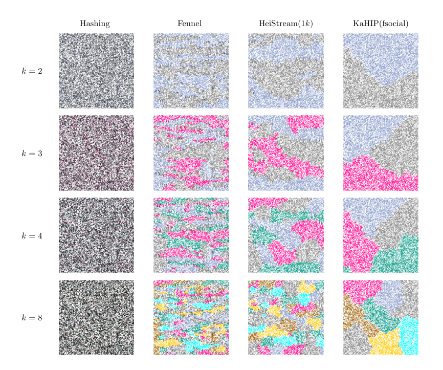
Visualization. As shown, the edge-cut of partitions produced by HeiStream is on average lower than the edge-cut of partitions produced by its competitor streaming algorithms. We shortly look at some visualizations in order to concretely understand why this happens. In Figure 9, we show a visual comparison of some partition layouts generated by Hashing, Fennel, HeiStream and the fast social version of KaHIP for the graph rgg15. Since this graph has only 32 768 nodes, we use a buffer size of 1 024 nodes for HeiStream in order to partition the graph over multiple successive batches. There is a leap of partitioning quality from Hashing to Fennel, i. e., well-delimited clusters associated to a same block can be identified in the partitions generated by Fennel but not in partitions generated by Hashing. Similarly there is a leap of partitioning quality from Fennel to KaHIP, i. e., a block generated by Fennel consists of multiple small clusters that are not mutually connected while a block generated by KaHIP usually consists of a single connected cluster. Note that the partitions produced by HeiStream have intermediary characteristics between the partitions generated by Fennel and KaHIP. More specifically, a block generated by HeiStream consists of fewer and larger clusters than a block generated by Fennel but not as few and as large clusters as those generated by KaHIP. This behavior is a direct consequence of the more or less global view provided by the distinct computational models used by these three algorithms.
4.3. Huge Graphs
| Graph | k | HeiStream(Xk) | Fennel | LDG | Hashing | |||||
|---|---|---|---|---|---|---|---|---|---|---|
| X | CE(%) | RT(s) | CE(%) | RT(s) | CE(%) | RT(s) | CE(%) | RT(s) | ||
| uk-2005 | 8 | 1024 | 4.03 | 290.23 | 19.93 | 37.19 | 19.97 | 19.36 | 73.70 | 3.28 |
| 16 | 1024 | 6.01 | 300.04 | 22.76 | 58.05 | 22.72 | 22.58 | 78.86 | 3.38 | |
| 32 | 1024 | 7.65 | 310.72 | 25.24 | 98.78 | 25.19 | 29.19 | 81.39 | 3.30 | |
| 64 | 1024 | 8.99 | 322.14 | 26.88 | 183.15 | 26.81 | 42.90 | 82.60 | 3.28 | |
| 128 | 1024 | 9.94 | 346.73 | 27.89 | 342.74 | 27.76 | 61.87 | 83.18 | 3.27 | |
| 256 | 1024 | 10.68 | 386.64 | 28.78 | 666.22 | 28.65 | 109.20 | 83.46 | 3.31 | |
| twitter7 | 8 | 512 | 41.64 | 1727.13 | 45.18 | 184.17 | 56.11 | 180.85 | 71.66 | 3.46 |
| 16 | 512 | 47.04 | 1774.92 | 53.49 | 213.17 | 61.73 | 186.27 | 76.78 | 3.57 | |
| 32 | 512 | 52.59 | 1884.16 | 58.15 | 244.18 | 66.84 | 184.90 | 79.34 | 3.49 | |
| 64 | 512 | 57.53 | 1988.11 | 62.95 | 330.46 | 68.68 | 197.86 | 80.62 | 3.50 | |
| 128 | 512 | 61.87 | 2113.34 | 66.68 | 504.53 | 69.94 | 219.65 | 81.26 | 3.93 | |
| 256 | 512 | 65.47 | 2357.92 | 78.32 | 846.20 | 71.26 | 280.99 | 81.57 | 3.51 | |
| sk-2005 | 8 | 1024 | 3.23 | 634.79 | 21.95 | 55.39 | 21.13 | 30.98 | 81.50 | 4.17 |
| 16 | 1024 | 4.11 | 648.48 | 26.36 | 82.41 | 25.33 | 35.44 | 87.26 | 4.20 | |
| 32 | 1024 | 5.32 | 667.84 | 29.59 | 137.42 | 27.97 | 43.76 | 90.11 | 4.23 | |
| 64 | 1024 | 7.55 | 695.60 | 32.52 | 238.54 | 30.18 | 59.19 | 91.50 | 4.21 | |
| 128 | 1024 | 8.95 | 733.05 | 35.87 | 449.19 | 32.44 | 91.36 | 92.19 | 4.20 | |
| 256 | 1024 | 12.02 | 798.73 | 40.06 | 857.76 | 35.69 | 150.64 | 92.55 | 4.26 | |
| soc-friendster | 8 | 1024 | 27.36 | 4099.35 | 30.57 | 405.68 | 45.60 | 381.78 | 87.53 | 5.45 |
| 16 | 1024 | 34.50 | 4202.04 | 45.74 | 440.11 | 58.98 | 361.54 | 93.77 | 5.62 | |
| 32 | 1024 | 39.52 | 4345.96 | 54.87 | 503.90 | 61.00 | 408.56 | 96.89 | 5.49 | |
| 64 | 1024 | 46.35 | 4546.98 | 59.27 | 649.34 | 64.02 | 422.87 | 98.45 | 5.44 | |
| 128 | 1024 | 52.41 | 4796.56 | 60.82 | 888.14 | 68.17 | 475.16 | 99.22 | 5.72 | |
| 256 | 1024 | 57.79 | 5323.08 | 64.25 | 1426.16 | 71.90 | 523.66 | 99.61 | 5.53 | |
| er-fact1.5s26 | 8 | 1024 | 73.27 | 2216.99 | 73.44 | 259.98 | 73.44 | 208.81 | 87.50 | 5.57 |
| 16 | 1024 | 80.18 | 2292.12 | 80.40 | 288.90 | 80.40 | 226.01 | 93.75 | 5.57 | |
| 32 | 1024 | 84.36 | 2400.35 | 84.63 | 357.21 | 84.63 | 255.60 | 96.87 | 5.60 | |
| 64 | 1024 | 86.99 | 2534.09 | 87.31 | 506.23 | 87.31 | 270.58 | 98.44 | 5.58 | |
| 128 | 1024 | 88.72 | 2725.81 | 89.10 | 769.61 | 89.10 | 407.59 | 99.22 | 5.57 | |
| 256 | 1024 | 89.99 | 2913.95 | 90.45 | 1329.57 | 90.45 | 408.35 | 99.61 | 5.65 | |
| RHG1 | 8 | 1024 | 0.04 | 380.04 | 2.02 | 86.95 | 2.02 | 44.42 | 91.91 | 8.37 |
| 16 | 1024 | 0.06 | 391.63 | 2.12 | 143.47 | 2.12 | 52.11 | 97.39 | 8.57 | |
| 32 | 1024 | 0.09 | 406.56 | 2.16 | 252.15 | 2.16 | 65.65 | 99.19 | 8.38 | |
| 64 | 1024 | 0.15 | 435.71 | 2.17 | 450.73 | 2.17 | 95.22 | 99.74 | 8.33 | |
| 128 | 1024 | 0.22 | 482.06 | 2.18 | 877.69 | 2.18 | 147.22 | 99.90 | 8.31 | |
| 256 | 1024 | 0.34 | 569.77 | 2.19 | 1708.33 | 2.18 | 273.76 | 99.95 | 8.45 | |
| RHG2 | 8 | 1024 | 0.09 | 621.56 | 0.05 | 103.83 | 0.04 | 56.23 | 89.71 | 8.31 |
| 16 | 1024 | 0.13 | 632.61 | 0.07 | 153.29 | 0.04 | 60.14 | 96.15 | 8.57 | |
| 32 | 1024 | 0.19 | 648.68 | 0.12 | 262.91 | 0.05 | 77.34 | 98.73 | 9.85 | |
| 64 | 1024 | 0.29 | 674.36 | 0.18 | 468.04 | 0.05 | 108.39 | 99.57 | 8.32 | |
| 128 | 1024 | 0.44 | 727.66 | 0.28 | 872.68 | 0.07 | 157.75 | 99.85 | 8.31 | |
| 256 | 1024 | 0.68 | 816.60 | 0.44 | 1686.18 | 0.09 | 278.51 | 99.92 | 8.47 | |
| uk-2007-05 | 8 | 1024 | 0.54 | 1024.26 | 25.23 | 107.46 | 25.21 | 58.19 | 87.91 | 8.80 |
| 16 | 1024 | 0.60 | 1045.36 | 28.02 | 166.06 | 28.19 | 70.72 | 94.08 | 8.79 | |
| 32 | 1024 | 0.70 | 1058.73 | 29.40 | 278.38 | 29.32 | 85.42 | 97.12 | 8.99 | |
| 64 | 1024 | 0.92 | 1099.64 | 29.94 | 517.20 | 29.85 | 115.18 | 98.61 | 9.32 | |
| 128 | 1024 | 1.31 | 1163.45 | 30.73 | 935.98 | 30.18 | 175.01 | 99.33 | 8.79 | |
| 256 | 1024 | 1.95 | 1280.48 | 31.65 | 1808.52 | 30.70 | 324.71 | 99.68 | 8.92 | |
We now switch to the main use case of streaming algorithms: computing high-quality partitions for huge graphs on small machines. The experiments in this section are based on the huge graphs listed in Table 1 and are run on the relatively small Machine B. Namely, we ran experiments for and we did not repeat each test multiple times with different seeds as in previous experiments. We also ran Metis and KaHIP on those graphs on this machine, but they fail on all instances since they require more memory than the machine has. For all instances, HeiStream performs a single pass over the input based on the extended model construction. We refer to setups of HeiStream with specific buffer sizes as HeiStream(k), in which a buffer contains nodes. In Table 3, we report detailed per-instance results with large buffer sizes able to run on Machine B. We exclude from Table 3 the IO delay to load the input graph from the disk, since it depends on the disk and is roughly the same independently of the used partitioning algorithm. For completeness, we report this delay (in seconds) for the huge graphs listed in Table 1 following their respective order: 131.3, 203.2, 313.2, 294.0, 164.9, 186.1, 340.7, 551.5.
The results show that HeiStream outperforms all the competitor algorithms regarding solution quality for most instances. Notably, HeiStream computes partitions with considerably lower edge-cut in comparison to the one-pass algorithms for 4 out of the tested graphs: uk-2005, sk-2005, uk-2007-05, and RHG1. For the social networks soc-friendster and twitter7, HeiStream is the best for all instances, but the improvement over Fennel and LDG is not so large as in the other instances. One outlier can be seen on the network RHG2. While HeiStream produces fairly small edge-cut values, which are all below , Fennel does outperform both and LDG improves solution quality even further on this instance. Furthermore, note that the running time of Fennel increases with increasing to the point in which it becomes higher than the running time of HeiStream for 5 out of the 8 huge graphs tested.
Memory Consumption.
We now shortly review the amount of memory needed by the streaming algorithms under consideration. First of all note that the memory of HeiStream depends on the size of the buffer that is used. If the buffer only contains one node, then the memory requirements match those of Fennel and LDG. Here, we measure the memory consumption of HeiStream for various buffer sizes and compare it to Fennel and LDG. To do that, we measured the memory consumption of HeiStream(1024k), HeiStream(32k), Fennel and LDG on the three largest graphs (RHG1, RHG2, and uk-2007-05). On average, HeiStream(1024k) consumes respectively , , and of memory to partition these graphs. while HeiStream(32k) consumes , , and , and Fennel and LDG use , , and . Note that the increased amount of used memory of HeiStream(1024k) is expected, since we use a fairly large buffer. Given the size of the graphs, we believe those required amounts of memory are more than reasonable.
5. Conclusion
We proposed HeiStream, a buffered streaming graph partitioning algorithm. We combined the buffered streaming model with multilevel graph partitioning techniques and extended Fennel to a multilevel algorithm. Compared to the previous state of-the-art of streaming graph partitioning, HeiStream computes significantly better solutions than known streaming algorithms while at the same time being faster in many cases. Note that improved edge cuts directly improve the communication cost in applications such as online queries on distributed graph databases (Pacaci and Özsu 2019). Hence, our results directly yield improvements in applications. An important property of HeiStream is that its running time does not depend on the number of blocks, while the previous state-of-the-art streaming partitioning algorithms have running time almost proportional to this number of blocks.
Acknowledgements.
Partially supported by DFG grant SCHU 2567/1-2.References
- (1)
- Awadelkarim and Ugander (2020) Amel Awadelkarim and Johan Ugander. 2020. Prioritized Restreaming Algorithms for Balanced Graph Partitioning. In Proceedings of the 26th ACM SIGKDD International Conference on Knowledge Discovery & Data Mining. 1877–1887. https://doi.org/10.1145/3394486.3403239
- Bader et al. (2014) D. A. Bader, H. Meyerhenke, P. Sanders, C. Schulz, A. Kappes, and D. Wagner. 2014. Benchmarking for Graph Clustering and Partitioning. In Encyclopedia of Social Network Analysis and Mining. Springer, 73–82. https://doi.org/10.1007/978-1-4939-7131-2_23
- Bichot and Siarry (2011) C. Bichot and P. Siarry (Eds.). 2011. Graph Partitioning. Wiley. https://doi.org/10.1002/9781118601181
- Brandes et al. (2007) Ulrik Brandes, Daniel Delling, Marco Gaertler, Robert Gorke, Martin Hoefer, Zoran Nikoloski, and Dorothea Wagner. 2007. On modularity clustering. IEEE transactions on knowledge and data engineering 20, 2 (2007), 172–188. https://doi.org/10.1109/TKDE.2007.190689
- Bui and Jones (1992) T. N. Bui and C. Jones. 1992. Finding Good Approximate Vertex and Edge Partitions is NP-Hard. IPL 42, 3 (1992), 153–159. https://doi.org/10.1016/0020-0190(92)90140-Q
- Buluç et al. (2016) Aydın Buluç, Henning Meyerhenke, Ilya Safro, Peter Sanders, and Christian Schulz. 2016. Recent Advances in Graph Partitioning. Springer International Publishing, Cham, 117–158. https://doi.org/10.1007/978-3-319-49487-6_4
- Carbone et al. (2015) Paris Carbone, Asterios Katsifodimos, Stephan Ewen, Volker Markl, Seif Haridi, and Kostas Tzoumas. 2015. Apache flink: Stream and batch processing in a single engine. Bulletin of the IEEE Computer Society Technical Committee on Data Engineering 36, 4 (2015).
- Cheng et al. (2012) Raymond Cheng, Ji Hong, Aapo Kyrola, Youshan Miao, Xuetian Weng, Ming Wu, Fan Yang, Lidong Zhou, Feng Zhao, and Enhong Chen. 2012. Kineograph: taking the pulse of a fast-changing and connected world. In Proceedings of the 7th ACM european conference on Computer Systems. 85–98. https://doi.org/10.1145/2168836.2168846
- Ching et al. (2015) Avery Ching, Sergey Edunov, Maja Kabiljo, Dionysios Logothetis, and Sambavi Muthukrishnan. 2015. One trillion edges: Graph processing at facebook-scale. Proceedings of the VLDB Endowment 8, 12 (2015), 1804–1815. https://doi.org/10.14778/2824032.2824077
- Dean and Ghemawat (2008) Jeffrey Dean and Sanjay Ghemawat. 2008. MapReduce: simplified data processing on large clusters. Commun. ACM 51, 1 (2008), 107–113. https://doi.org/10.1145/1327452.1327492
- Demirci et al. (2019) Gunduz Vehbi Demirci, Hakan Ferhatosmanoglu, and Cevdet Aykanat. 2019. Cascade-aware partitioning of large graph databases. VLDB J. 28, 3 (2019), 329–350. https://doi.org/10.1007/s00778-018-0531-8
- Funke et al. (2019) Daniel Funke, Sebastian Lamm, Ulrich Meyer, Manuel Penschuck, Peter Sanders, Christian Schulz, Darren Strash, and Moritz von Looz. 2019. Communication-free massively distributed graph generation. J. Parallel and Distrib. Comput. 131 (2019), 200–217.
- Garey et al. (1974) M. R. Garey, D. S. Johnson, and L. Stockmeyer. 1974. Some Simplified NP-Complete Problems. In Proc. of the 6th ACM Symposium on Theory of Computing ((STOC)). ACM, 47–63. https://doi.org/10.1145/800119.803884
- Gonzalez et al. (2012) Joseph E Gonzalez, Yucheng Low, Haijie Gu, Danny Bickson, and Carlos Guestrin. 2012. Powergraph: Distributed graph-parallel computation on natural graphs. In Presented as part of the 10th USENIX Symposium on Operating Systems Design and Implementation (OSDI 12). 17–30. https://doi.org/10.5555/2387880.2387883
- Hendrickson and Leland (1995) B. Hendrickson and R. Leland. 1995. A Multilevel Algorithm for Partitioning Graphs. In Proc. of the ACM/IEEE Conference on Supercomputing’95. ACM, Article 28. https://doi.org/10.1145/224170.224228
- Holtgrewe et al. (2010) M. Holtgrewe, P. Sanders, and C. Schulz. 2010. Engineering a Scalable High Quality Graph Partitioner. Proc. of the 24th IPDPS (2010), 1–12.
- Jafari et al. (2021) Nazanin Jafari, Oguz Selvitopi, and Cevdet Aykanat. 2021. Fast shared-memory streaming multilevel graph partitioning. J. Parallel and Distrib. Comput. 147 (2021), 140–151. https://doi.org/10.1016/j.jpdc.2020.09.004
- Karypis and Kumar (1998) G. Karypis and V. Kumar. 1998. A Fast and High Quality Multilevel Scheme for Partitioning Irregular Graphs. SIAM Journal on Scientific Computing 20, 1 (1998), 359–392.
- Leskovec and Krevl (2014) Jure Leskovec and Andrej Krevl. 2014. SNAP Datasets: Stanford Large Network Dataset Collection. http://snap.stanford.edu/data.
- Malewicz et al. (2010) Grzegorz Malewicz, Matthew H Austern, Aart JC Bik, James C Dehnert, Ilan Horn, Naty Leiser, and Grzegorz Czajkowski. 2010. Pregel: a system for large-scale graph processing. In Proceedings of the 2010 ACM SIGMOD International Conference on Management of data. 135–146. https://doi.org/10.1145/1807167.1807184
- Mayer et al. (2018) Christian Mayer, Ruben Mayer, Muhammad Adnan Tariq, Heiko Geppert, Larissa Laich, Lukas Rieger, and Kurt Rothermel. 2018. Adwise: Adaptive window-based streaming edge partitioning for high-speed graph processing. In 2018 IEEE 38th International Conference on Distributed Computing Systems (ICDCS). IEEE, 685–695. https://doi.org/10.1109/ICDCS.2018.00072
- Meyerhenke et al. (2014) H. Meyerhenke, P. Sanders, and C. Schulz. 2014. Partitioning Complex Networks via Size-constrained Clustering, In 13th Int. Symp. on Exp. Algorithms. preprint arXiv:1402.3281 8504. https://doi.org/10.1007/978-3-319-07959-2_30
- Nishimura and Ugander (2013) Joel Nishimura and Johan Ugander. 2013. Restreaming graph partitioning: simple versatile algorithms for advanced balancing. In Proceedings of the 19th ACM SIGKDD international conference on Knowledge discovery and data mining. 1106–1114. https://doi.org/10.1145/2487575.2487696
- Pacaci and Özsu (2019) Anil Pacaci and M Tamer Özsu. 2019. Experimental Analysis of Streaming Algorithms for Graph Partitioning. In Proceedings of the 2019 International Conference on Management of Data. 1375–1392. https://doi.org/10.1145/3299869.3300076
- Patwary et al. (2019) Md Anwarul Kaium Patwary, Saurabh Garg, and Byeong Kang. 2019. Window-based streaming graph partitioning algorithm. In Proceedings of the Australasian Computer Science Week Multiconference. 1–10. https://doi.org/10.1145/3290688.3290711
- Penschuck et al. (2020) Manuel Penschuck, Ulrik Brandes, Michael Hamann, Sebastian Lamm, Ulrich Meyer, Ilya Safro, Peter Sanders, and Christian Schulz. 2020. Recent Advances in Scalable Network Generation. CoRR abs/2003.00736 (2020). arXiv:2003.00736 https://arxiv.org/abs/2003.00736
- Petroni et al. (2015) Fabio Petroni, Leonardo Querzoni, Khuzaima Daudjee, Shahin Kamali, and Giorgio Iacoboni. 2015. Hdrf: Stream-based partitioning for power-law graphs. In Proceedings of the 24th ACM International on Conference on Information and Knowledge Management. 243–252. https://doi.org/10.1145/2806416.2806424
- Raghavan et al. (2007) U. N. Raghavan, R. Albert, and S. Kumara. 2007. Near Linear Time Algorithm to Detect Community Structures in Large-Scale Networks. Physical Review E 76, 3 (2007), 036106. https://doi.org/10.1103/PhysRevE.76.036106
- Rossi and Ahmed (2015) Ryan A. Rossi and Nesreen K. Ahmed. 2015. The Network Data Repository with Interactive Graph Analytics and Visualization. http://networkrepository.com.
- Sajjad et al. (2016) Hooman Peiro Sajjad, Amir H Payberah, Fatemeh Rahimian, Vladimir Vlassov, and Seif Haridi. 2016. Boosting vertex-cut partitioning for streaming graphs. In 2016 IEEE International Congress on Big Data (BigData Congress). IEEE, 1–8. https://doi.org/10.1109/BigDataCongress.2016.10
- Sanders and Schulz (2011) P. Sanders and C. Schulz. 2011. Engineering Multilevel Graph Partitioning Algorithms. In Proc. of the 19th European Symp. on Algorithms (LNCS, Vol. 6942). Springer, 469–480. https://doi.org/10.1007/978-3-642-23719-5_40
- Schulz and Strash (2019) C. Schulz and D. Strash. 2019. Graph Partitioning: Formulations and Applications to Big Data. In Encyclopedia of Big Data Technologies. https://doi.org/10.1007/978-3-319-63962-8_312-2
- Stanton and Kliot (2012) Isabelle Stanton and Gabriel Kliot. 2012. Streaming graph partitioning for large distributed graphs. In Proceedings of the 18th ACM SIGKDD international conference on Knowledge discovery and data mining. 1222–1230. https://doi.org/10.1145/2339530.2339722
- Tsourakakis et al. (2014) Charalampos Tsourakakis, Christos Gkantsidis, Bozidar Radunovic, and Milan Vojnovic. 2014. Fennel: Streaming graph partitioning for massive scale graphs. In Proceedings of the 7th ACM international conference on Web search and data mining. 333–342. https://doi.org/10.1145/2556195.2556213