Some continuous and discontinuous Galerkin methods and structure preservation for incompressible flows
Abstract
In this paper, we present consistent and inconsistent discontinous Galerkin methods for incompressible Euler and Navier-Stokes equations with the kinematic pressure, Bernoulli function and EMAC function. Semi- and fully discrete energy stability of the proposed dG methods are proved in a unified fashion. Conservation of total energy, linear and angular momentum is discussed with both central and upwind fluxes. Numerical experiments are presented to demonstrate our findings and compare our schemes with conventional schemes in the literature in both unsteady and steady problems. Numerical results show that global conservation of the physical quantities may not be enough to demonstrate the performance of the schemes, and our schemes are competitive and able to capture essential physical features in several benchmark problems.
Keywords:
incompressible flows, discontinuous Galerkin method, mixed finite element method , energy stability , pressure robustness , structure preservation1 Introduction
There has been extensive research on Galerkin methods for incompressible flows, see, e.g., [50, 21, 26, 33, 17] and references therein. Since the pressure is usually viewed as a Lagrange multiplier, it could be naturally decoupled from the velocity by restricting the problem on the divergence-free subspace [22, 2] at the continuous level. Since the discrete divergence-free subspace is often not contained in the continuous one, classical -conforming methods suffer from a loss of numerical accuracy as the velocity error is affected by the pressure approximation, especially under small viscosity, which is known in the literature as a lack of pressure robustness [28]. In the current paper, we focus on ways to reduce the influences of pressure approximations on velocity approximations. With the help of a grad-div stabilization term [20], one may increase pressure robustness although the mass conservation is violated, see, e.g., [28, 42, 41, 39, 43, 7, 37, 27]. Another remedy is to use -conforming methods that completely remove pressure influence on the velocity approximation through a carefully chosen finite element pair [45, 5, 3]. In this case, the numerical velocity is pointwise divergence-free [28, 25, 47, 51, 18, 24, 35]. Moreover, in the vorticity-stream formulation, one could automatically enforce the divergence-free constraint at the PDE level when the spatial dimension is two [21, 38, 6]. Finally, for discontinuous Galerkin (dG) methods, a common technique for pressure robustness is penalizing the jump of the velocity normal component [25, 1, 29, 23]. An interesting result is reported in [49], where an element-wise grad-div penalization was used on tensor product meshes for a non-isothermal flow, and an improvement of the mass conservation is observed for an inf-sup stable element pair of equal order. A discrete inf-sup condition involving the pressure jump is constructed in [17] for both the steady incompressible Stokes and Navier-Stokes equations. In [36], reconstruction with the lowest-order divergence-free Raviart-Thomas velocity is used to recover the -orthogonality of the discretely divergence-free velocities and irrotational vector fields. Other relevant dG methods can be found in e.g., [15, 8, 16].
In this paper, we generalize our previous work [12] and present two new classes of dG methods for incompressible Euler and Navier-Stokes equations. The unified numerical framework in [12] is designed for incompressible Navier-Stokes equations with the kinematic pressure . Here, this approach is further extended to cover the Bernoulli function , and EMAC function . The Bernoulli function is roughly speaking the “force” one feels when one faces into the wind, an important physical quantity rarely considered as a direct output in computational fluids. The EMAC function was first proposed in [9] for conserving energy, linear and angular momentum by -conforming finite element methods. We refer to [10, 31, 44, 48] and references therein for more discussions about these two functions.
In addition, we shall show that both classes of dG methods achieve the same numerical velocity field when the velocity is -conforming, and we shall analyze their conservation property for energy, linear momentum and angular momentum with both central and upwind fluxes. To the best of our knowledge, such frameworks and conservation analysis for -conforming and dG methods do not exist in the literature. From our dG framework, it is also shown that global energy conservation for inviscid flows is generally not worth pursuing at the expense of pressure robustness. Nevertheless, all proposed methods in this framework are proved to be energy stable in the fully-discrete level, which is an important property in the simulation of turbulent flows (cf. [19]).
2 Preliminaries
Let denote a conforming and shape-regular simplicial mesh on a polyhedral domain in with . Let denote the collection of faces of , the set of interior faces, and the set of boundary faces. For and , we use to denote the diameter of , the diameter of . For any -dimensional set , let denote the inner product on , and
Given , we fix a unit normal to , which points from one element to the other element on the other side. The jump and averaging operators are defined as
where and are arbitrary scalar- and vector-valued functions, respectively. For a boundary face which is contained in a single element , we further assume that is the outward pointing normal to and define
Throughout the rest of this paper, we use to denote the piecewise constant vector defined on the skeleton such that for all Let denote the space of polynomials of degree at most (with a non-negative integer). We shall make use of the following function spaces
where or corresponding to the Raviart–Thomas (RT) [45] or Brezzi–Douglas–Marini (BDM) [5] shape function space, respectively.
The rest of this paper is organized as follows. In Section 3, we first present the unified framework and then prove the semi- and fully-discrete stability of the general scheme for the incompressible Euler equations in the general form, then we briefly extend our schemes to the incompressible Navier-Stokes equations. In Section 4, we analysis the conservation properties of the -conforming and dG methods. In Section 5, we perform numerical experiments to confirm our findings in Section 4 and test our dG schemes in both unsteady and steady situations, and compare the results with conventional schemes in the literature. Finally we conclude our paper in Section 6.
3 Incompressible Euler Equations
Consider the incompressible Euler equations in the following form
| (1) | ||||
where is defined as
| (2) |
with being an arbitrary constant. Note that unifies the kinematic pressure (), Bernoulli function () and EMAC function (). Although the EMAC function is not a physical quantity, its corresponding formulation could be used to calculate the numerical velocity.
Let denote the inner product on and the broken gradient with respect to . For the form with , we follow the derivation in [12] and obtain a semi-discrete scheme: Find unknowns for each time such that
| (3a) | ||||
| (3b) | ||||
for all . The penalty term is defined as
| (4) |
for some constant , which is used to increase pressure robustness. The numerical flux is
where are user-specified piecewise non-negative constants controlling the amount of numerical dissipation. Using element-wise integration by parts, the scheme (3) becomes
| (5a) | ||||
| (5b) | ||||
where
| (6) | ||||
| (7) |
However, the form is inconsistent when . In general, for , our semi-discrete scheme for (1) seeks such that
| (8a) | ||||
| (8b) | ||||
The term coincides with if and will be specified later if . In particular, we want where approximates
A key observation is that in (6) is an approximation to . Therefore for the new term in (1), its variational counterpart 11 1 Here the property of matrix transposition is used. could be discretized as
Here we discard the term in as it lacks physical meaning.
- 1.
Scheme dG1
Based on the above analysis, we introduce
(9) The corresponding scheme (8) with is denoted as dG1. The advantage is that the positivity of is closely related to the positive structure of . Unfortunately, is inconsistent due to the two terms and .
Remark 1
The inconsistent dG1 scheme is the starting point of our framework and is conveniently derived from an existing discrete convective form without redoing tedious integration-by-parts. Later we shall develop another dG method to enforce consistency. Furthermore, derivations of the embedded - and -conforming methods become transparent by imposing stronger continuity on dG spaces.
Let us define the kernel of as
Then restricting (8a) with to yields
(10) Using Cauchy-Schwarz inequality, we have
It follows that one could choose sufficiently large penalizing parameter in to control , , and in turn to minimize the inconsistent terms , , which are variational crimes. Therefore, the consistency of dG1 is weakly enforced. We will show through numerical experiments in Section 5 that one may choose properly to achieve high numerical accuracy. We note that the inconsistent terms will have an effect on the approximation of as the penalization is enforced in . However, in many physical problems involving incompressible flows, the velocity is usually the physical quantity of interest. Furthermore, in the EMAC case has no physical meaning, and is naturally consistent for the case of the kinematic pressure when . Therefore, the only physically meaningful expression of affected by the inconsistency is the Bernoulli function corresponding to . This observation motivates the following new class of dG methods.
- 2.
Scheme dG2
To guarantee the consistency of (8), we discard the two inconsistent terms in (9) and present an alternative convective form
(11) The corresponding scheme (8) with is denoted by dG2. Direct calculation shows that dG2 is consistent. Coefficients of the second and fourth terms in are modified for stability analysis, see Lemma 1 for details.
In particular, in (11) for the Bernoulli function () and EMAC function () reduces to
and
respectively.
- 3.
Scheme Hdiv
Replacing with in (8) and taking or yields an conforming numerical scheme (denoted as Hdiv) for (1). It is well-known that is an inf-sup stable pair and . Hence the incompressibility holds pointwise via (8b). Another essential feature of is that on . Then the penalty term of Hdiv vanishes for any . Let . Restricting to , for all the convective form for Hdiv satisfies
(12) where , and are used. Therefore, dG1 and dG2 recover the same numerical velocity when the velocity is -conforming. They generalize the conforming method in [11], where the recovery of the same numerical velocity is discussed and shown experimentally under the setting of -conforming with consistent formulation.
So far, we obtain two new DG schemes dG1 and dG2, where dG2 is exactly consistent and dG1 is weakly consistent by penalization. In addition, dG1 and dG2 reduce to the H(div) conforming scheme Hdiv provided is replaced with .
Lemma 1 (Positivity of and )
Assume for all when or assume be arbitrary non-negative number when then we have
Proof 1
Direct calculation confirms the following identities
It follows that
Using (9), (11), and the previous equation, we have
| (14) | ||||
Finally, we conclude the proof by using for when or by using the boundary condition of when it belongs to .
∎
Now we are in a position to present the following semi-discrete stability.
Theorem 1 (Semi-discrete Stability Estimate)
Let the assumption in Lemma 1 hold. Then for all , Schemes dG1, dG2, and Hdiv satisfy
Proof 2
∎
We use the Crank-Nicolson scheme to discretize the time direction. Let the time interval be partitioned into . Let and
Let be a suitable interpolation of . The fully discrete scheme for (1) is to find such that for all
| (15a) | ||||
| (15b) | ||||
where or When is replaced by , (15) is the fully discrete Hdiv scheme. In (15), and approximate and , respectively. The next theorem confirms the stability of (15).
Theorem 2 (Fully Discrete Energy Estimate)
Let the assumptions in Theorem 1 hold. We have
Proof 3
∎
The stability of is guaranteed by a discrete inf-sup condition on , see, e.g., [1].
Remark 2
Consider the incompressible Navier-Stokes equations
where To discretize the term we introduce the following viscous bilinear form
where is a user-specified parameter, and The bilinear form is standard in the context of interior penalty dG methods, see, e.g., [4]. Now it is straightforward to extend the scheme (15) to the Navier-Stokes equations: Find such that
| (17a) | ||||
| (17b) | ||||
The corresponding stability result is an direct extension of our previous analysis for the incompressible Euler equations by observing that is coercive w.r.t. a mesh dependent norm, see, e.g., [13, 17] for a detailed discussion.
Remark 3
Error estimates of -conforming and dG methods for the incompressible Euler equations can be found in [11, 25, 40]. For incompressible Navier-Stokes equations, interested readers are referred to [33, 47]. It is worth noticing that error estimation of -conforming methods in [33] assumes the existence of an -bounded Stokes projection, which is generally hard to prove. On the other hand, the error estimates of dG methods for Euler equations in [25] reply on a postprocessed -conforming velocity. Without normal continuity of the velocity and post-processing procedures, the error analysis of dG methods in this paper is expected to be even more difficult. We refer to [47] for interesting discussions on some open problems about error estimates for incompressible Navier-Stokes equations.
4 Conservation of Physical Quantities
In this section, we discuss the conservation properties of the proposed scheme (15). In particular we are interested in the conservation of discrete energy, linear and angular momentum of dG1, dG2, and Hdiv.
Theorem 3 (Energy Conservation)
Proof 4
From Lemma 1, Eqs. (4) and (16), we observe that the only possibility that the total energy is conserved is when both and vanish. Clearly implies . In view of (14), implies Finally, stability condition for implies that can only be 1.
For the H(div) scheme, recall that . Then energy conservation is equivalent to
The proof is complete.
∎
We use to weakly enforce the consistency of Scheme dG1. Hence the requirement does not make sense in practice for dG1. For dG2, indicates a lack of pressure robustness. Therefore we do not believe the conservation of energy (at the sacrifice of pressure robustness) is worth pursuing in the dG formulations within the current framework, actually numerical experiments show that both the Newton nonlinear solver with the MUMPS linear solver or with the GMRES linear solver break down after a few time steps.
We then consider the preservation of discrete linear and angular momentum. Straightforward calculations show that dG schemes do not conserve the linear and angular momentum. For the H(div) scheme, the test function (for linear momentum) or (for angular momentum) is not contained in , where is the -th unit vector. Following [9], we assume that and in an inner neighborhood of the boundary and take Given a continuous function , we take on and to be suitably defined to meet the boundary condition. Integration by parts yields
where we have used pointwise, and is continous within . Using again, we have
| (18) |
Taking in (18), it follows that
| (19) |
For and any function , elementary tensor calculation shows that . Therefore (18) with implies
| (20) |
As a consequence, we obtain the next theorem.
Theorem 4 (Linear and Angular Momentum Conservation-(div))
Proof 5
Let be or within and arbitrarily defined in to meet the boundary condition. Clearly we have
| (21) |
and thus in Then using and the assumption , (15a) reduces to
The preservation of linear () and angular momentum () is equivalent to . For simplicity of presentation, we omit the superscript of in the rest of the proof.
It is noted that may not belong to . Therefore one could not directly make use of (12), (19) and (20) to conclude
Instead one need to study and separately. We recall that (12) implies all -conforming scheme recover the same numerical velocity, and the linear and angular moment only depend on the velocity field. Hence it is enough to analyze and .
- 1.
The case of
- 2.
The case of
Remark 4
The upwinding H(div) scheme () fails to preserve the total energy. However it is interesting to see that the upwinding H(div) scheme still conserves the linear- and angular momentum.
5 Numerical Experiments
In this section, we present numerical simulations to test the conservation properties of the Hdiv schemes (15), and the performance of the dG schemes (15) and (17) in steady and unsteady problems with being either (dG1) or (dG2), and . The viscous penalization parameter is taken as while and are specified in each example. In each experiment, we use the non-homogeneous Dirichlet boundary condition and weakly enforce it via modifying the right hand side of (15) or (17). Our numerical simulations are performed in FEniCS [32], an open-source computing platform for solving partial differential equations using finite element methods. For all numerical experiments in this section, we use the Newton nonlinear solver with the MUMPS linear solver inside FEniCS to solve the nonlinear systems of equations arising from fully discrete schemes. The absolute and relative error tolerances in the Newton solver are set to be for dynamic problems and for stationary problems.
5.1 Conservation Test
In this subsection, we use the problem of Gresho vortex [9] to test the conservation properties of the Hdiv scheme (15) with both (central flux) and (upwind flux) using BDM element for . The space domain is with the initial velocity and kinematic pressure fields described by
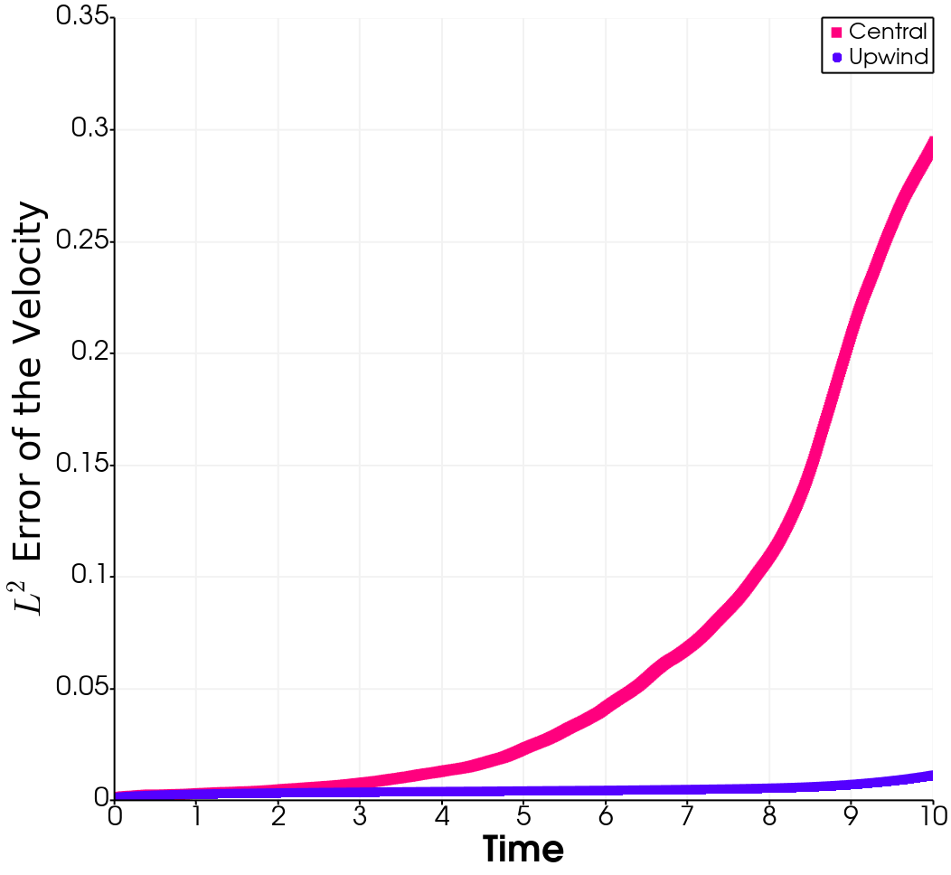
Here polar coordinates are used, and and . Note that the initial state is an exact solution of the steady incompressible Euler equations, therefore an accurate scheme should preserve the solution when there is no forcing terms. For this problem, we run the simulation with and for with time step . From Figures 1 and 3, we have the following interesting observations
- 1.
Both upwind and central fluxes seem to be able to conserve the total linear momentum in both and directions.
- 2.
Energy dissipation appears when upwinding since , but the maximum relative error of total energy is less than , which is almost negligible.
- 3.
Compared to upwind flux, the central flux fails to conserve the total angular momentum after about . This is due to the violation of the assumption near , which is also confirmed by the left column of Figure 3. However, one thing worth noticing is that the maximum relative error of angular momentum for central flux is within , acceptable for most engineering applications. Therefore one may consider the central flux being able to conserve the angular momentum.
- 4.
Central fluxes have a much larger (more than times) error in the velocity compared with upwind flux. Figure 3 indicates that central flux fails to preserve the right physics after about and makes almost no physical sense when , although all global conservation properties hold up to (if one’s tolerance of relative error is within ).
Through this example, we show that the conservation of global physical quantities such as energy, linear and angular momentum may not be a good indicator for a well-behaved numerical scheme as they lack the control of local behaviors, which could be as bad as the left figure in the lower row of Figure 3. In addition, we have shown that the upwinding H(div) scheme could numerically preserve linear and angular momentum, as predicted by our theoretical analysis, and this point has not been seriously discussed in the literature.




5.2 Accuracy of Scheme dG2
In this subsection, we test the behavior of Scheme dG2 and compare it with the classical scheme from [1, 17] using the Taylor-Green vortex and the Kovasznay flow problems, which are popular benchmark problems in computational fluid dynamics [25, 14, 38, 17]. More precisely, Taylor-Green vortex is used with the incompressible Euler equations with the viscous terms viewed as a forcing term, while Kovasznay flow is used as an exact solution to the incompressible Navier-Stokes equations. Throughout the rest of the paper, we set .
We first study the Taylor-Green vortex in , with the analytical solution given by [25]
The space domain is , which is meshed with squares and each square was further split into two congruent triangles. We set , and run the simulation for using the time step on meshes with mesh sizes and polynomial degree . Finally, we record the formulation in [17] below, which is
Note that the scheme in [17] is designed only for steady flows with not necessarily being positive semi-definite. Therefore this scheme is not proved to be energy stable for unsteady flow.
| d.o.f | Our Schemes | Scheme in [1, 17] Error order | ||||||
|---|---|---|---|---|---|---|---|---|
|
|
| ||||||
| 0 | 0.8886 | 1401 | 2.02e-1 — | 2.02e-1 — | 2.02e-1 — | 2.01e-1 — | ||
| 0.4443 | 5601 | 4.44e-2 2.18 | 4.44e-2 2.18 | 4.45e-2 2.18 | 4.44e-2 2.18 | |||
| 0.2221 | 22041 | 1.03e-2 2.11 | 1.03e-2 2.11 | 1.03e-2 2.11 | 1.03e-2 2.11 | |||
| 0.1777 | 35001 | 6.50e-3 2.06 | 6.50e-3 2.06 | 6.51e-3 2.06 | 6.50e-3 2.06 | |||
| 1 | 0.8886 | 3001 | 2.04e-2 — | 2.04e-2 — | 2.04e-2 — | 2.04e-2 — | ||
| 0.4443 | 12001 | 3.05e-3 2.74 | 3.05e-3 2.74 | 3.05e-3 2.74 | 3.05e-3 2.74 | |||
| 0.2221 | 48001 | 3.98e-4 2.94 | 3.98e-4 2.94 | 3.99e-4 2.93 | 3.98e-4 2.94 | |||
| 0.1777 | 75001 | 2.04e-4 2.99 | 2.04e-4 2.99 | 2.05e-4 2.99 | 2.04e-4 2.99 | |||
| 2 | 0.8886 | 5201 | 1.40e-3 — | 1.40e-3 — | 1.40e-3 — | 1.40e-3 — | ||
| 0.4443 | 20801 | 8.06e-5 4.12 | 8.05e-5 4.12 | 8.10e-5 4.11 | 8.05e-5 4.12 | |||
| 0.2221 | 83201 | 4.94e-6 4.03 | 4.93e-6 4.03 | 4.97e-6 4.03 | 4.93e-6 4.03 | |||
| 0.1777 | 130001 | 2.01e-6 4.02 | 2.01e-6 4.02 | 2.03e-6 4.01 | 2.01e-6 4.02 | |||
From Table 1, we observe that all schemes achieve the expected order of convergence and roughly the same level of accuracy.
Next, we study the Kovasznay flow with the analytical solution given by [17]
Here and . The simulation domain is set to be . All schemes are tested with and polynomial degree on uniform meshes with mesh size .
| d.o.f | Our schemes | Scheme in [1, 17] Error order | ||||||
|---|---|---|---|---|---|---|---|---|
|
|
| ||||||
| 0 | 0.2828 | 1401 | 9.26e-2 — | 9.26e-2 — | 9.27e-2 — | 1.49e-1 — | ||
| 0.1414 | 5601 | 2.40e-2 1.95 | 2.40e-2 1.95 | 2.40e-2 1.95 | 2.98e-2 2.33 | |||
| 0.0707 | 22041 | 6.13e-3 1.97 | 6.13e-3 1.97 | 6.14e-3 1.97 | 6.53e-3 2.19 | |||
| 0.0566 | 35001 | 3.95e-3 1.97 | 3.95e-3 1.97 | 3.95e-3 1.97 | 4.11e-3 2.08 | |||
| 1 | 0.2828 | 3001 | 1.08e-2 — | 1.08e-2 — | 1.08e-2 — | 1.12e-2 — | ||
| 0.1414 | 12001 | 1.35e-3 3.01 | 1.35e-3 3.01 | 1.35e-3 3.01 | 1.35e-3 3.06 | |||
| 0.0707 | 48001 | 1.68e-4 3.00 | 1.68e-4 3.00 | 1.68e-4 3.00 | 1.68e-4 3.00 | |||
| 0.0566 | 75001 | 8.58e-5 3.00 | 8.57e-5 3.00 | 8.58e-5 3.00 | 8.57e-5 3.00 | |||
| 2 | 0.2828 | 5201 | 8.93e-4 — | 8.93e-4 — | 8.93e-4 — | 8.92e-4 — | ||
| 0.1414 | 20801 | 5.82e-5 3.94 | 5.82e-5 3.94 | 5.82e-5 3.94 | 5.82e-5 3.94 | |||
| 0.0707 | 83201 | 3.73e-6 3.96 | 3.73e-6 3.96 | 3.73e-6 3.96 | 3.73e-6 3.96 | |||
| 0.0566 | 130001 | 1.55e-6 3.95 | 1.55e-6 3.95 | 1.55e-6 3.95 | 1.55e-6 3.95 | |||
From Table 2, we observe that all four schemes have the expected order of convergence. The three versions of our scheme achieve roughly the same level of accuracy, and relatively smaller absolute errors compared with scheme in [17] especially when .
In summary, the consistent formulation dG2 is comparable to classical dG schemes in the literature.
5.3 Temporal Accuracy Test
In this subsection, we use the following two-dimensional unsteady flow to investigate the temporal accuracy of our schemes [30]
The computational domain is and is set to be . We focus on the dG2 with and for simplicity of presentation. Simulations are performed with polynomial degree , mesh size , time steps , and the total simulation time . It could be observed from Table 3 that the Crank-Nicolson time discretization has reasonable second order accuracy.
| Order | |||
|---|---|---|---|
| 1 | 0.01s | 1.62e-5 | — |
| 0.02s | 6.42e-5 | 1.99 | |
| 0.04s | 2.55e-4 | 1.99 | |
| 0.08s | 1.19e-3 | 2.23 | |
| 2 | 0.01s | 1.61e-5 | — |
| 0.02s | 6.41e-5 | 2.00 | |
| 0.04s | 2.55e-4 | 1.99 | |
| 0.08s | 1.19e-3 | 2.23 |
5.4 Accuracy of Scheme dG1
In this subsection, we use Taylor-Green vortex and Kovasznay problems to study the behavior of the dG1 formulation with respect to . For simplicity, we focus on the case when . The basic setting is as in Subsection 5.2. Note that is used to increase pressure robustness in the consistent formulation dG2. However, dG1 is not consistent and is additionally used for weakly enforcing consistency. The main purpose here is to study the numerical influence of on dG1.
In Table 4, we observe a decrease of absolute velocity errors when increases, and optimal convergence when for the Taylor-Green vortex. It can be observed from Figure 4 that weird contours of vorticity when are cured by increasing to and . The improved numerical performance of dG1 as grows is due to the enhanced consistency and pressure robustness by larger . Further comparison between the corresponding columns in Tables 1 and 4 indicates that a larger is needed to maintain the same level of accuracy as in the dG2 formulation, especially when .
In the case of the Kovasznay flow, the dG1 and dG2 formulations achieve roughly the same level of accuracy with for all values of . In the high resolution case , , , there is an abnormal reduction on the rate of convergence. We point out that this phenomenon could be fixed by further reducing the absolute and relative tolerances to in the Newton solver. A possible explanation is that the condition number of the stiffness matrix with of the linearized equations is significantly larger than stiffness matrices with , and thus smaller iterative error tolerances are needed to recover numerical accuracy. When using coarse meshes and lower order polynomials (common in practice), we still recommended to use large . The observed different numerical behaviors with respect to in steady and unsteady cases shed some light in the difference between stationary and evolutionary problems.
| d.o.f | ||||||||
|---|---|---|---|---|---|---|---|---|
|
|
| ||||||
| 0 | 0.8886 | 1401 | 4.89e-1 — | 2.02e-1 — | 1.82e-1 — | |||
| 0.4443 | 5601 | 2.73e-1 8.42e-1 | 4.44e-2 2.18 | 4.35e-2 2.06 | ||||
| 0.2221 | 22401 | 1.85e-1 5.65e-1 | 1.03e-2 2.11 | 1.02e-2 2.09 | ||||
| 0.1777 | 35001 | 1.65e-1 5.00e-1 | 6.51e-3 2.06 | 6.48e-3 2.05 | ||||
| 1 | 0.8886 | 3001 | 2.36e-1 — | 2.04e-2 — | 2.00e-2 — | |||
| 0.4443 | 12001 | 1.74e-1 4.42e-1 | 3.03e-3 2.75 | 3.04e-3 2.72 | ||||
| 0.2221 | 48001 | 1.25e-1 4.70e-1 | 4.37e-4 2.79 | 3.98e-4 2.93 | ||||
| 0.1777 | 75001 | 1.13e-1 4.82e-1 | 2.70e-4 2.16 | 2.04e-4 2.99 | ||||
| 2 | 0.8886 | 5201 | 1.75e-1 — | 1.42e-3 — | 1.39e-3 — | |||
| 0.4443 | 20801 | 1.26e-1 4.70e-1 | 2.21e-4 2.68 | 8.05e-5 4.11 | ||||
| 0.2221 | 83201 | 9.02e-2 4.85e-1 | 1.48e-4 5.79e-1 | 4.93e-6 4.03 | ||||
| 0.1777 | 130001 | 8.09e-2 4.90e-1 | 1.33e-4 4.91e-1 | 2.01e-6 4.02 | ||||


| d.o.f | ||||||||
|---|---|---|---|---|---|---|---|---|
|
|
| ||||||
| 0 | 0.2828 | 1401 | 1.40e-1 — | 9.26e-2 — | 9.26e-2 — | |||
| 0.1414 | 5601 | 4.35e-2 1.69 | 2.40e-2 1.95 | 2.40e-2 1.95 | ||||
| 0.0707 | 22401 | 1.15e-2 1.92 | 6.13e-3 1.97 | 6.23e-3 1.95 | ||||
| 0.0566 | 35001 | 7.44e-3 1.93 | 3.95e-3 1.97 | 4.12e-3 1.84 | ||||
| 1 | 0.2828 | 3001 | 1.92e-2 — | 1.08e-2 — | 1.08e-2 — | |||
| 0.1414 | 12001 | 6.10e-3 1.65 | 1.35e-3 3.01 | 1.35e-3 3.01 | ||||
| 0.0707 | 48001 | 2.20e-3 1.47 | 1.68e-4 3.00 | 1.27e-3 8.86e-2 | ||||
| 0.0566 | 75001 | 1.54e-3 1.61 | 8.59e-5 3.00 | 1.26e-3 3.78e-2 | ||||
| 2 | 0.2828 | 5201 | 7.71e-3 — | 8.94e-4 — | 8.93e-4 — | |||
| 0.1414 | 20801 | 2.52e-3 1.61 | 5.85e-5 3.93 | 5.82e-5 3.94 | ||||
| 0.0707 | 83201 | 8.14e-4 1.63 | 3.90e-6 3.91 | 1.25e-3 -4.42 | ||||
| 0.0566 | 130001 | 5.72e-4 1.58 | 1.72e-6 3.67 | 1.25e-3 | ||||
5.5 Flow Over a Cylinder and Lid Driven Flow by dG1
In the last subsection, we continue to study the behavior of the dG1 formulation for the problems of flow over a cylinder [34, 46, 32] and lid driven flow when and . The goal is to check whether the scheme could capture the essential physical features of such flows. Recall that dG1 is not a consistent formulation by nature, and its consistency is weakly imposed through .
We first study the flow over a cylinder. A primary feature of this problem is the formation of von Kármán vortex street, which depends on both the spatial and temporal discretizations. Therefore the ability to have vortex properly generated is not trivial, see, e.g., [12, 34] for numerical examples failing to have this property. The domain is set to be with a disk centered at and of radius . We run the simulation for using a time step . The flow is subjected to the following inflow and outflow profile ([34])
and vanishing velocity on the rest of . The viscosity is set to be , and therefore the mean Reynolds number ranges from to .
From Figure 6, we observe that dG1 is able to recover the vortex formation successfully.
Finally, we consider the lid driven flow on the square domain with a tangential velocity on the top and vanishing velocity on the other sides. We are interested in the flow with , which has a large gradient near the lid due to the singularities introduced by the jump of the velocity on the top two corners, and the recovery of the small corner vortex is essential.


Figure 7 shows that dG1 is able to capture the essential features of the lid driven flow.
From Subsections 5.4 and 5.5, we observe that the inconsistent dG1 formulation actually works well when choosing sufficiently large parameter . This fact was explained by our argument below equation (10). In particular, experiments show that with properly chosen , one could still achieve high numerical accuracy and capture essential physical features.
6 Conclusion
We developed two classes of dG methods for the incompressible Euler and incompressible Navier-Stokes equations with the kinematic pressure, Bernoulli function and EMAC function with both semi- and fully discrete stability. When the velocity is -conforming, we show that central flux conserves energy, linear momentum and angular momentum, while upwind flux conserves linear momentum and angular momentum under appropriate assumptions. Numerical experiments were performed to demonstrate our findings, test the performances of the schemes, and compare with conventional schemes in the literature. When the velocity is -conforming, the simulation results show that global conservation of physical quantities is not enough to guarantee the performance of the schemes, since they are not good indicators of the local behaviors. For the dG schemes, our schemes tend to achieve smaller absolute error when in Kovasznay flow, while achieve roughly the same order of accuracy otherwise in both the Taylor-Green vortex and Kovasznay flows when scheme dG2 is considered. Temporal accuracy test shows that the Crank-Nicolson time discretization indeed has second order accuracy. Furthermore, we also show through numerical examples that fairly accurate results for velocity could be obtained when the scheme dG1 formulation is used with the Bernoulli function with a suitable penalization. The observation of locking in the Kovasznay flow indicates the important difference in the finite element schemes for steady and unsteady problems. Finally, with the problems of flow around a cylinder and lid driven flow, we show that dG1 is able to capture the essential physics of the problem when the governing equations are with the Bernoulli function.
Data Availability Statement
The data that support the findings of this study are available from the corresponding author upon reasonable request.
References
- [1] Mine Akbas, Alexander Linke, Leo G. Rebholz, and Philipp W. Schroeder, The analogue of grad–div stabilization in DG methods for incompressible flows: Limiting behavior and extension to tensor-product meshes, Computer Methods in Applied Mechanics and Engineering 341 (2018), 917–938.
- [2] Grégoire Allaire and Grègoire Allaire, Numerical analysis and optimization: an introduction to mathematical modelling and numerical simulation, Oxford university press, 2007.
- [3] Daniele Boffi, Franco Brezzi, and Michel Fortin, Mixed finite element methods and applications, vol. 44, Springer, 2013.
- [4] Susanne C. Brenner and L. Ridgway Scott, The mathematical theory of finite element methods, third ed., Texts in Applied Mathematics, vol. 15, Springer, New York, 2008. MR 2373954
- [5] Franco Brezzi, Jim Douglas, Jr., and L. D. Marini, Two families of mixed finite elements for second order elliptic problems, Numer. Math. 47 (1985), no. 2, 217–235. MR 799685
- [6] Xiaofeng Cai, Wei Guo, and Jing-Mei Qiu, A high order semi-Lagrangian discontinuous Galerkin method for the two-dimensional incompressible Euler equations and the guiding center Vlasov model without operator splitting, Journal of Scientific Computing 79 (2019), no. 2, 1111–1134.
- [7] Michael A. Case, Vincent J. Ervin, Alexander Linke, and Leo G. Rebholz, A connection between Scott–Vogelius and grad-div stabilized Taylor–Hood FE approximations of the Navier–Stokes equations, SIAM Journal on Numerical Analysis 49 (2011), no. 4, 1461–1481.
- [8] Aycil Cesmelioglu, Bernardo Cockburn, and Weifeng Qiu, Analysis of a hybridizable discontinuous Galerkin method for the steady-state incompressible Navier-Stokes equations, Mathematics of Computation 86 (2017), no. 306, 1643–1670.
- [9] Sergey Charnyi, Timo Heister, Maxim A. Olshanskii, and Leo G. Rebholz, On conservation laws of Navier–Stokes Galerkin discretizations, Journal of Computational Physics 337 (2017), 289–308.
- [10] Sergey Charnyi, Timo Heister, Maxim A Olshanskii, and Leo G Rebholz, Efficient discretizations for the EMAC formulation of the incompressible Navier–Stokes equations, Applied Numerical Mathematics 141 (2019), 220–233.
- [11] Xi Chen and Corina Drapaca, H (div) conforming methods for the rotation form of the incompressible fluid equations, Calcolo 57 (2020), no. 4, 1–26.
- [12] Xi Chen, Yuwen Li, Corina Drapaca, and John Cimbala, A unified framework of continuous and discontinuous Galerkin methods for solving the incompressible Navier–Stokes equation, Journal of Computational Physics, DOI: 10.1016/j.jcp.2020.109799 (2020).
- [13] Xi Chen and David M Williams, Versatile mixed methods for the incompressible navier-stokes equations, arXiv preprint arXiv:2007.08015 (2020).
- [14] Alexandre Joel Chorin, Numerical solution of the Navier-Stokes equations, Mathematics of computation 22 (1968), no. 104, 745–762.
- [15] Bernardo Cockburn, Guido Kanschat, and Dominik Schötzau, A locally conservative LDG method for the incompressible Navier-Stokes equations, Mathematics of Computation 74 (2005), no. 251, 1067–1095.
- [16] , A note on discontinuous Galerkin divergence-free solutions of the Navier–Stokes equations, Journal of Scientific Computing 31 (2007), no. 1-2, 61–73.
- [17] Daniele Antonio Di Pietro and Alexandre Ern, Mathematical aspects of discontinuous Galerkin methods, Mathématiques & Applications (Berlin) [Mathematics & Applications], vol. 69, Springer, Heidelberg, 2012. MR 2882148
- [18] Richard S. Falk and Michael Neilan, Stokes complexes and the construction of stable finite elements with pointwise mass conservation, SIAM Journal on Numerical Analysis 51 (2013), no. 2, 1308–1326.
- [19] Niklas Fehn, Wolfgang A Wall, and Martin Kronbichler, Robust and efficient discontinuous Galerkin methods for under-resolved turbulent incompressible flows, Journal of Computational Physics 372 (2018), 667–693.
- [20] Leopoldo P. Franca and Thomas J. R. Hughes, Two classes of mixed finite element methods, Computer Methods in Applied Mechanics and Engineering 69 (1988), no. 1, 89–129.
- [21] Vivette Girault and Pierre-Arnaud Raviart, Finite element methods for Navier-Stokes equations, Springer Series in Computational Mathematics, vol. 5, Springer-Verlag, Berlin, 1986, Theory and algorithms. MR 851383
- [22] , Finite element methods for Navier-Stokes equations: theory and algorithms, vol. 5, Springer Science & Business Media, 2012.
- [23] Philip M. Gresho and Stevens T. Chan, On the theory of semi-implicit projection methods for viscous incompressible flow and its implementation via a finite element method that also introduces a nearly consistent mass matrix. part 2: Implementation, International Journal for Numerical Methods in Fluids 11 (1990), no. 5, 621–659.
- [24] Johnny Guzmán and Michael Neilan, Conforming and divergence-free Stokes elements on general triangular meshes, Mathematics of Computation 83 (2014), no. 285, 15–36.
- [25] Johnny Guzmán, Chi-Wang Shu, and Filánder A. Sequeira, H(div) conforming and DG methods for incompressible Euler’s equations, IMA Journal of Numerical Analysis 37 (2016), no. 4, 1733–1771.
- [26] Jan S. Hesthaven and Tim Warburton, Nodal discontinuous Galerkin methods: Algorithms, analysis, and applications, Springer Science & Business Media, 2007.
- [27] Eleanor W. Jenkins, Volker John, Alexander Linke, and Leo G. Rebholz, On the parameter choice in grad-div stabilization for the Stokes equations, Advances in Computational Mathematics 40 (2014), no. 2, 491–516.
- [28] Volker John, Alexander Linke, Christian Merdon, Michael Neilan, and Leo G. Rebholz, On the divergence constraint in mixed finite element methods for incompressible flows, SIAM Review 59 (2017), no. 3, 492–544.
- [29] Sumedh M. Joshi, Peter J. Diamessis, Derek T. Steinmoeller, Marek Stastna, and Greg N. Thomsen, A post-processing technique for stabilizing the discontinuous pressure projection operator in marginally-resolved incompressible inviscid flow, Computers & Fluids 139 (2016), 120–129.
- [30] Dongjoo Kim and Haecheon Choi, A second-order time-accurate finite volume method for unsteady incompressible flow on hybrid unstructured grids, Journal of computational physics 162 (2000), no. 2, 411–428.
- [31] Pijush K Kundu, I Cohen, and D Dowling, Fluid mechanics. 1990, Google Scholar, 56–59.
- [32] Hans Petter Langtangen and Anders Logg, Solving PDEs in Python, Springer, 2017.
- [33] William Layton, Introduction to the Numerical Analysis of Incompressible Viscous Flows, SIAM, 2008.
- [34] William Layton, Carolina C. Manica, Monika Neda, Maxim Olshanskii, and Leo G. Rebholz, On the accuracy of the rotation form in simulations of the Navier–Stokes equations, Journal of Computational Physics 228 (2009), no. 9, 3433–3447.
- [35] Christoph Lehrenfeld and Joachim Schöberl, High order exactly divergence-free hybrid discontinuous Galerkin methods for unsteady incompressible flows, Computer Methods in Applied Mechanics and Engineering 307 (2016), 339–361.
- [36] Alexander Linke, On the role of the Helmholtz decomposition in mixed methods for incompressible flows and a new variational crime, Computer methods in applied mechanics and engineering 268 (2014), 782–800.
- [37] Alexander Linke, Leo G. Rebholz, and Nicholas E. Wilson, On the convergence rate of grad-div stabilized Taylor–Hood to Scott–Vogelius solutions for incompressible flow problems, Journal of Mathematical Analysis and Applications 381 (2011), no. 2, 612–626.
- [38] Jian-Guo Liu and Chi-Wang Shu, A high-order discontinuous Galerkin method for 2d incompressible flows, Journal of Computational Physics 160 (2000), no. 2, 577–596.
- [39] Gert Lube and Maxim A. Olshanskii, Stable finite-element calculation of incompressible flows using the rotation form of convection, IMA Journal of Numerical Analysis 22 (2002), no. 3, 437–461.
- [40] Andrea Natale and Colin J Cotter, A variational finite-element discretization approach for perfect incompressible fluids, IMA Journal of Numerical Analysis 38 (2018), no. 3, 1388–1419.
- [41] Maxim Olshanskii, Gert Lube, Timo Heister, and Johannes Löwe, Grad–div stabilization and subgrid pressure models for the incompressible Navier–Stokes equations, Computer Methods in Applied Mechanics and Engineering 198 (2009), no. 49-52, 3975–3988.
- [42] Maxim Olshanskii and Arnold Reusken, Grad-div stablilization for Stokes equations, Mathematics of Computation 73 (2004), no. 248, 1699–1718.
- [43] Maxim A. Olshanskii, A low order Galerkin finite element method for the Navier–Stokes equations of steady incompressible flow: a stabilization issue and iterative methods, Computer Methods in Applied Mechanics and Engineering 191 (2002), no. 47-48, 5515–5536.
- [44] Maxim A Olshanskii and Leo G Rebholz, Longer time accuracy for incompressible Navier-Stokes simulations with the EMAC formulation, arXiv preprint arXiv:2002.01416 (2020).
- [45] P.-A. Raviart and J. M. Thomas, A mixed finite element method for 2nd order elliptic problems, Mathematical aspects of finite element methods (Proc. Conf., Consiglio Naz. delle Ricerche (C.N.R.), Rome, 1975), 1977, pp. 292–315. Lecture Notes in Math., Vol. 606. MR 0483555
- [46] Michael Schäfer, Stefan Turek, Franz Durst, Egon Krause, and Rolf Rannacher, Benchmark computations of laminar flow around a cylinder, Flow simulation with high-performance computers II, Springer, 1996, pp. 547–566.
- [47] Philipp W. Schroeder, Christoph Lehrenfeld, Alexander Linke, and Gert Lube, Towards computable flows and robust estimates for inf-sup stable FEM applied to the time-dependent incompressible Navier–Stokes equations, SeMA Journal, Boletin de la Sociedad Española de Matemática Aplicada 75 (2018), no. 4, 629–653.
- [48] Philipp W Schroeder and Gert Lube, Pressure-robust analysis of divergence-free and conforming FEM for evolutionary incompressible Navier–Stokes flows, Journal of Numerical Mathematics (2017).
- [49] Philipp W. Schroeder and Gert Lube, Stabilised dG-FEM for incompressible natural convection flows with boundary and moving interior layers on non-adapted meshes, Journal of Computational Physics 335 (2017), 760–779.
- [50] Roger Temam, Navier-Stokes equations, third ed., Studies in Mathematics and its Applications, vol. 2, North-Holland Publishing Co., Amsterdam, 1984, Theory and numerical analysis, With an appendix by F. Thomasset. MR 769654
- [51] Shangyou Zhang, A new family of stable mixed finite elements for the 3D Stokes equations, Mathematics of Computation 74 (2005), no. 250, 543–554.