Analysis of EEG data using complex geometric structurization
Abstract
Electroencephalogram (EEG) is a common tool used to understand brain activities. The data are typically obtained by placing electrodes at the surface of the scalp and recording the oscillations of currents passing through the electrodes. These oscillations can sometimes lead to various interpretations, depending on the subject’s health condition, the experiment carried out, the sensitivity of the tools used, human manipulations etc. The data obtained over time can be considered a time series. There is evidence in the literature that epilepsy EEG data may be chaotic. Either way, the embedding theory in dynamical systems suggests that time series from a complex system could be used to reconstruct its phase space under proper conditions. In this paper, we propose an analysis of epilepsy electroencephalogram time series data based on a novel approach dubbed complex geometric structurization. Complex geometric structurization stems from the construction of strange attractors using embedding theory from dynamical systems. The complex geometric structures are themselves obtained using a geometry tool, namely the -shapes from shape analysis. Initial analyses show a proof of concept in that these complex structures capture the expected changes brain in lobes under consideration. Further, a deeper analysis suggests that these complex structures can be used as biomarkers for seizure changes.
Keywords: EEG, time series, complex structure, morphometry, alpha-shape
1 Introduction
In neuroscience, to understand brain functions and brain related diseases, it is very common to place electrodes on a subject’s head and record the electrical activities that result. These activities, when represented, are often oscillations that change in shape, frequency, and range. They can be analyzed to see if meaningful information can be extracted that gives a clue about the brain state of the subject at a certain time, or in a certain region of the brain. The accuracy of the recording highly depends on the instrument used, the region of interest (ROI), the experimenter’s experience, the time of the day, the subject’s discipline during the recording and many other factors. This is to say that uncertainty in the accuracy of the information recorded is always present. Even when the information is being recorded on the same subject, on the same day, on the same ROI, but at different intervals, changes are bound to occur. Electroencephalogram or EEG, a term coined by Berger 1929, are electrical activities recorded on humans or animals that display prominent oscillatory behavior subject to important changes during various behavioral states. These changes show a high degree of nonlinearity in the signals that may be important. Indeed, in the field of biomedical signal processing (analysis of heart rate variability, electrocardiogram, hand tremor, EEG), the presence or absence of nonlinearity often conveys information about the health condition of a subject. In particular, EEG signals are often examined using nonlinearity analysis techniques or by comparing signals that are recorded during different physiological brain states (e.g. epileptic seizure). The differences observed during these analyses can either be due to genuine differences in dynamical properties of the brain or due to differences in recording parameters. The EEG are often analyzed as times series and there are many methods for analysis of times series in the literature. The methods can be grouped into two categories: univariate measures and multivariate measures. A good review on the topic can be found in Carney et al. 2011.
Among the methods that have been touted as more efficient at providing an insight into the real dynamics of EEG is the famous Embedding Theorem of Takens 1981. This Embedding Theorem has been instrumental to understanding how to reconstruct the true dynamics of systems based on the times series measured on these systems. Essentially, this reconstruction theory, in layman’s terms, suggests that a times series measured over sufficiently long period of times contains enough information to reconstruct the phase space in which the associated system normally evolves. This allows also to show that there are other intricate subunits that influence the changes observed in the measured variables that are represented in the time series. This theorem was used for example by Grassberger and Procaccia 1983 to propose a measure called Correlation Dimension which was in turn instrumental to Lehnertz and Elger 1998 for the prediction of epilepsy seizures. Despite all the methods proposed in the literature, there is no agreement on which method constitutes the best tool at extracting the most meaningful information that could be useful for the physician for the prediction of seizure-like diseases. Moreover, with the increasing use of the concepts of chaos and complexity in health sciences, it is becoming more and more difficult to distinguish their adequate application. For example, there have been evidence of chaos in EEG data, see Destexhe and Babloyantz 1986; Destexhe 1992; Destexhe et al. 1998, and since chaotic systems are inherently complicated, they may look complex. Likewise, complex systems may also look chaotic. Distinguishing these two notions is important in applications, especially in health sciences. Henceforth, we will adopt a terminology along the lines of Rickles et al. 2007 for understanding complexity and chaos.
In this paper, we propose a new method for analyzing EEG times series data, which we call Complex Geometric Structurization (CGS). The complex nature of the method stems from the fact that we have multiple subunits interacting together resulting in a rich collective behavior feeding back into the behavior of individual parts. The method is inspired by the Embedding Theorem of Takens 1981 for the construction of a geometric structure whose volume can be evaluated from shape analysis technique. The volume of this geometric structure behaves as a key statistic akin to a biomarker for the phenomenon or ROI of interest. Using data driven approaches to study brain pathologies is a very active field of study nowadays due to improvement in life expectancy across the world with its cohorts of problems such as brain disorders as illustrated in Zheng et al. 2019, David et al. 2020 and the references therein. Moreover, the push to use data and methodological driven approaches to brain pathologies is also evidenced by the numerous grants offered by the National Institute of Health and private foundations such as the Michael J. Fox Foundation for Parkinson Disease, the Bill and Melinda Gates Foundations, just to name some.
The remainder of the paper is organized as follows: In Section 2, we make a brief review on how to use the Embedding Theorem to construct strange attractors; in Section 3, we review important notions of statistical morphometry; in Section 4, we introduce the complex geometric structurization method; in Section 5, we discuss some applications of the CGS method on real data; in Section 6, we discuss the pros and cons of the proposed method in different contexts.
2 Understanding Embedding Theory
As its name suggests, a dynamical system is a system whose variables evolve over time. Its phase space is a geometric representation of the trajectory of its variables over time. The values taken by the system’s variables at an instant describe the system’s states. To understand how to reconstruct the phase space of a dynamical system based on observations (times series) of one of its variables, we need to revisit the Embedding Theory of Takens 1981, which is essentially a high dimension transformation of the time series. Consider the -dimensional space . We recall that a manifold in the space is a topological space that locally looks like a Euclidian space near each point. Topology here means that bending is ignored. For example, the surface of the globe is a topological manifold in the space . Now, consider a dynamical system with a system’s state lying on a manifold of . Let be a sampling interval and let the time series be given as a one-dimensional observation of the system dynamics through an observation function . Takens 1981 embedding theory states that for almost every smooth function , the delay coordinate map defined as with is an embedding, that is, it is a one-to-one immersion of the state space attractor with dimension when . In other words, the result states that is a representative of , even if the true state space has not been observed, see Figure 1. The quantity is referred to in the literature as the embedding dimension and as the time delay (or lag). The embedding theory is predicated on the observation that a time series observed over a long period of time may show an internal structure. In fact, considering a time series , we only observe an incomplete picture of since is a scalar. However, if we observe it for a long period of time, a more precise description will emerge, which will help understand its dynamics. In practice, most of the focus is given into how to find appropriate values for the time delay and the embedding dimension , see Appendix 8.2. We observe that this type of reconstruction technique has been applied successfully in the case of epilepsy EEG data before, see for instance Destexhe and Babloyantz 1986, Destexhe 1992, and Destexhe et al. 1998.

2.1 Examples
Dynamical Systems: The Takens’ embedding theory can be used to reconstruct the Lorenz, a famous attractor often mentioned in dynamical systems. The Lorenz 1963 systems of differential equations is given as
It is known for example that the Lorenz system is chaotic for , and . Figure 2 below is a depiction of this attractor for these parameter values plotted in the space , and . The time step used is for an interval time of [0, 75] for the Lorenz system. We also note that the time lag or delay is , and was found using either the autocorrelation (ACF) or average mutual information (AMI), see for instance Section 8.2 below.

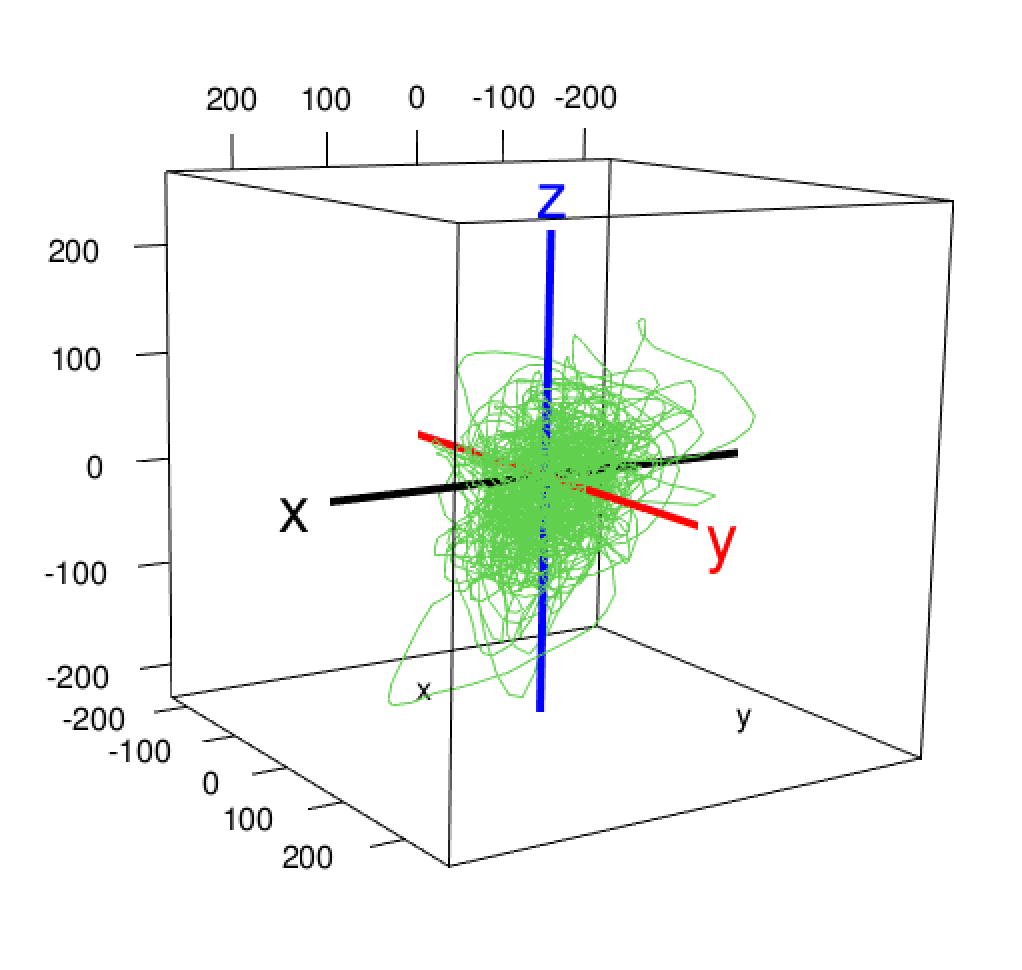
Real Data: There have been many applications of Takens’ embedding theory with real data. For example, in Fisher et al. 2009,Carney et al. 2011, an attractor is constructed from a publicly available (at http://www.meb.unibonn.de/epileptologie/science/physik/eegdata.html) epilepsy data set called here EDATA for simplicity. The data consist of five sets A, B, C, D, and E. Each containing 100 single-channel EEG segments of 23.6 seconds, each of which was selected after visual inspection for artifacts (such as acoustic and electrical shielding, separation of earth ground for laboratory, interconnectivity of devices on the same phase and ground centrally and locally) and has passed a weak stationarity criterion. Sets A and B were obtained from surface EEG recordings of five healthy subjects with eyes open and closed, respectively. Data were obtained in seizure-free intervals from five patients in the epileptogenic zone for set D and from the hippocampal formation of the opposite hemisphere of the brain for set C. Set E contains seizure activity, selected from all recording sites exhibiting ictal activity. Sets A and B have been recorded extracranially, whereas sets C, D, and E have been recorded intracranially. All EEG signals were recorded with the same 128-channel amplifier system, using an average common reference [omitting electrodes containing pathological activity (C,D, and E) or strong eye movement artifacts (A and B)]. After 12 bit analog-to-digital conversion, the data were written continuously onto the disk of a data acquisition computer system at a sampling rate of 173.61 Hz. Band-pass filter settings were 0.53–40 Hz (12 dB/oct.), see Andrzejak et al. 2001. Figure 3 below is an illustration of the dataset EDATA. Each row represents one time series from sets A, B, C, D, and E respectively. Clearly, time series in the seizure set E has a much pronounced amplitude synonymous with more brain activities. In Figure 4 below, we represent the reconstructed phase spaces based on the time selected times series from set A – E . We note that the axes are where , with ms.
| (A) | (B) |
|---|---|
 |
 |
| (C) | (D) |
 |
 |
| (E) | |
 |
3 Statistical Morphometry
Given a set of points in a two or three-dimensional space, statistical morphology (or morphometrics) amounts to finding an appropriate geometric characterization of the variability of the shape and size of the set of points. This characterization includes but is not limited to volumes and surface area, surface roughness, deviation from convexity, porosity, and permeability. We note that in general, the set of points may not be convex in the strictest sense, so there is a need for a method that relaxes the convexity restriction. The notions of -convexity and -shape represent alternatives that relax the strict convexity assumption. These new -shaped objects are even more flexible than -convex objects in that now controls the spatial scale of the estimator. note that is a unitless quantity. In fact, as decreases, the -shape shrinks and more space appears among the sample points, whereas as increases, the -shape object converges to the convex hull of the sample. In other words, in -shaped objects, controls the amount of porosity between the sample points. These -shaped objects have been used in various fields for the characterization of biological systems, see for instance Lafarge et al. 2014 and the references therein, or also Gardiner et al. 2018. We can mention the pivotal work of Edelsbrunner and Mücke 1994 where the main algorithm for the construction of -shaped objects can be found.
Example
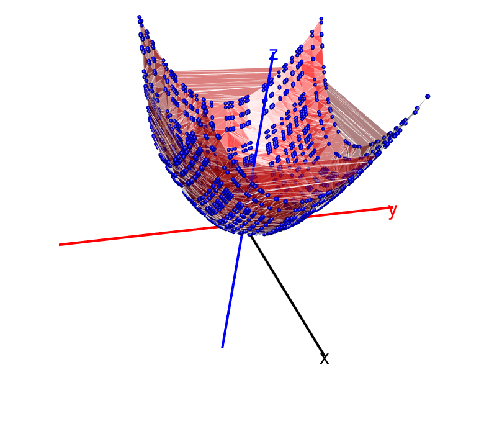
In the example below, we illustrate the -shape construction respectively in two and three dimension, based on a random sample of data taken from the original object .
We consider points in 3D, obtained from the object which is the object delimited by the curve and where and are random points selected in the interval . In Figure 5 below, we construct the -shape object (red) for (a), (b), (c), and (d).
| (a) | (b) | (c) | (d) |
|---|---|---|---|
 |
 |
 |
 |
4 Complex Geometric Structurization
In view of the apparent shape that can be observed from the reconstructed phase space above, the question of how to compare these complex structures arises. In other words, this question is related to the question of how to compare strange attractors. Among the methods proposed, we can mention the work of Grassberger and Procaccia 1983 and its many variants. The method we propose is borne out of the observation that there seems to be a complex geometric structure whose shape changes from healthy patients to seizure-prone ones. So we will rely on the notion of -shape to construct the complex structure related to each situation. We will use the following algorithm to construct our “complex structure” (CGS). The motivation comes from the fact that, given a time series, if it has been observed long enough, it carries the signature of the original phase space diagram in which the true system it originated from evolves. If we have many such time series from the same system, we should be able to capture enough information about the true phase space diagram. The large number of these time series should be enough to eventually eliminate noise or undesired artefacts from the reconstruction. We then expect each reconstructed phase diagram to be topologically equivalent to any other, therefore forming a structure compact enough to be the revolving center of all other reconstructed phase space diagram. In general, the the dimension of the space in which the true system evolves is greater than three, making it impossible to visualize with the naked-eye. Our empirical approach is to consider only a cross section of the reconstructed phase space in dimension three in this case. the reason for this choice is two-fold: one, we can actually visualize a part of the true phase space diagram. Second, we can use existing method to evaluate the volume of the structure in lower dimensions. This is to say that the volume is preserved in reconstruction. In doing this, we are trying to find a measurable identifier or markup for this group of time series that will vary from groups to groups and from individual to individual.
4.1 Explanation of the method
Given time series, we use the Takens reconstruction technique to obtain the embedding dimension (using ACF) and time delay (or sampling interval) for (using the method of false nearest neighbors). Let and . If , then for each time series, we obtain the complex structure CGSα(n). Let . We use the -shape technique to obtain the volume of the in 3D. This step is crucial since we choose to represent the complex structure only using the first three delay-coordinates even if the actual space has dimension . The motivation for this selection is that the volume of the CGS based on any combination of three coordinates would not significantly be different from any other volume obtained from any other combination of three coordinates. The reasoning behind the choice of is that the volume of the complex structure is bounded by the volume of its convex hull, as increases, so we select the smallest alpha that maximizes the volume, see section 4.4.3 below for an illustration. This leads to the following algorithm
4.2 Algorithm
- 1.
Use all the times series collected on patients in different groups.
- 2.
For each time series, reconstruct a 3D “strange attractor” from the first three delay-coordinates.
- 3.
Use the -shape technique to construct a “Complex Geometric Structure” (CGS) related to all strange attractors.
- 4.
Define a measure related to each CGS that that can be statistically analyzed. This could be the volume, the surface area, the center, etc.
- 5.
Repeat this procedure for all replicates (if there are any) and thus obtain new data.
- 6.
- (a)
For comparison:
Use a statistical test to see if there is a significant difference between measures of different groups. This could be a parametric or a nonparametric test. - (b)
For Prediction:
Use the data obtained for training in machine learning, see Kwessi and Edwards 2020 (preferred to standard generalized linear model (GLM) models because of the absence of a specific model) and test it on potential new data.
- (a)
4.3 Comments
- 1.
The CGS terminology stems from the fact the structures obtained after reconstruction do not have of classical geometric shapes. Their shapes are rather “complex” in nature.
- 2.
We propose to use all time series available for a particular region of the brain, at a specific instant; for example before seizure, during seizure, or after seizure. It is common to use one time series, see for instance Fisher et al. 2009. We note that repeated measures on the same subject do not yield the same values and thus in the reconstruction, there could be individual times series whose excursions in the phase space are wider than others yielding a bigger geometric structure in size and volume. In this case, individual times series could be used and the subsequent large volumes could be trimmed out if necessary. This is particularly important if one is interested for example in obtaining a richer data set to analyze.
- 3.
The embedding dimension often obtained is greater than 3, so in the absence of a visualization mechanism for data in spaces of dimensions higher than 3, we propose to focus on only the first three delay coordinates.
- 4.
Using the R-package Alphashape3d, measures such as volumes or surface areas can be obtained for the -shape object under consideration.
- 5.
As we saw in the example above, the choice of is critical in the -shape construction. We propose to select the minimum value of for which the volume is maximized.
- 6.
Finally, we note that in practice, the experimenter can used data from chaotic or complex systems. One can check for chaos in data by calculating Lyapunov exponents. If the data are sensitive to initial conditions and chaotic, the attractor would be referred to as a “strange attractor”, see Celso et al. 1987. Even if on the other hand the data are sensitive to initial conditions but non chaotic, we would still keep the same “strange attractor” denomination because in this case (the Lyapunov exponents are non-positive), the attractor obtained is still strange, see for instance Celso et al. 1984; Paladin and Vulpiani 1987. It also noteworthy to observe that non chaotic systems that are sensitive to initial conditions are sometimes referred to in the literature as complex systems, see for instance the comparative review between chaotic and complex systems by Rickles et al. 2007.
4.4 Technical considerations
In this section, we examine some technical considerations to keep in mind when implementing this method.
4.4.1 Choice of
As we mentioned above, the choice of is critical in this process. In what follows, we show that the optimal value of is smallest that maximizes the volume of the CGS. Moreover, if one is interested in comparing CGS among groups, it would be adequate to select a common value of , for example as the largest value, among the values that maximize the CGS for each group. For instance, using the EDATA set, we obtained and , with ms. In Figure 6 below, we observe that for a value of , the volume is maximized for the subset A, whereas the maximum is reached for subset E at . So, we will choose as the optimal value of if we want to compare the two CGSs.
4.4.2 Choice of the embedding dimension.
We note that the embedding dimension is closely related to the time lag. We are not going to discuss which should be estimated first. However, we note that there are two methods for estimating the time lag and they do not always yield the same embedding dimension. We propose to select the embedding dimension as the smallest value of the two embedding dimensions when they are different.
4.4.3 Choice of the delay-coordinates
In Section 4.4.2, we mentioned that we will select the first three delay-coordinates to construct the complex structure. However, it is worthwhile to consider the question of whether the volume would change if a different combination of delay-coordinates is used. Our choice is based on the conjecture that it does not matter which combination of delay-coordinates is selected. To emphasize that point, we will discuss the case of subsets A and E. In the case of subsets A and E, the embedding dimension found is . So there are possible different combinations of three delay-coordinates, selected among 10. So, for each combination, we will construct the corresponding CGS and assess whether the volume changes significantly across all the different CGS’s. Figure 7 shows the volume of the CGS by combination of three delay-coordinates for subsets A and E. The boxplots suggest that the distribution of volumes for each set is reasonably concentrated around its median (thick red and blue lines) with a small range and no outliers. This is to say that taking the first three delay coordinates seems reasonable despite minor variations otherwise.
| (A) | (E) |
|---|---|
The main takeaway from the plots above is that the variation of the volume as a function of the combination of delay-coordinates appear not to be significant. Even for seizure data like subset E, the variation in volume appears to be mild, which is our impetus for conjecturing that a similar observation could be made for other datasets. Obviously we cannot predict what will happen for all datasets, and ultimately that endeavor would require a mathematical proof that may go beyond the scope of the present manuscript.
5 Applications
5.1 Analysis of EDATA
In Figure 4, we have shown a representation of the reconstructed phase space diagram for one time series in the space and for each set A–E. In Figures 8–12, we construct the phase space diagram and the complex structures for the EDATA set, for all the 100 time series in each subset. We observe that for each set, we obtain a compact structure whose volume we can now evaluate, see (A1)–(E1). We selected for each case, because of all sets A-E, 580 is the value of alpha that maximizes the volume of the complex structure of E, the largest of all of them (see the selection criterion given above), see figure 6 above. The CGS structure for each set is then obtained, see (A2)–(E2). We observe that the CGS for set E appears to be bigger than all other CGSs, which is a sign of larger excursions in the phase space and therefore synonymous with a much intense brain activity during seizure.
| (A1) | (A2) |
|---|---|
 |
 |
| (B1) | (B2) |
|---|---|
 |
 |
| (C1) | (C2) |
|---|---|
 |
 |
| (D1) | (D2) |
|---|---|
 |
 |
| (E1) | (E2) | ||
|---|---|---|---|
 |
 |
Pooling the data may seem to inflate the volume of the CGS. So instead, we could construct the complex structure related to individual channel and evaluate their volumes. This will give a richer data to analyze, where outliers can be removed. Figure 13 below shows the boxplot of the volume of the complex structure for each channel. The volume for subset E is very large compared to A-E and obscures the distribution for subsets A-D. As a result, in the 2nd panel in Figure 13 we remove subset E so that the distributions of subsets A-D can be more clearly seen.
This Figure is further evidence of what already observable in the raw data in Figure 3 and Figure 4. Sets A–D have comparable amplitude at the time series level confirmed by the fact that the volume of CGS are in similar range. The amplitude at the time series level of Set E is much higher than that of sets A–D, which is also confirmed by a larger volume at CGS level. This is further evidence that during seizure, these volumes increase substantially when compared to seizure-free intervals. More importantly, we can extract meaningful statistics from this data as suggested in Table 1 below:
| Min | Median | Max | Mean | SD | |||
| A | 12.30 | 63.63 | 115.87 | 154.17 | 317.88 | 109.84 | 66.08 |
| B | 37.89 | 63.63 | 173.50 | 291.31 | 479.06 | 364.25 | 266.63 |
| C | 7.73 | 68.38 | 161.30 | 262.70 | 351.60 | 262.10 | 333.70 |
| D | 9.45 | 62.78 | 174.10 | 4569.00 | 17800.00 | 692.30 | 206.54 |
| E | 516.3 | 3277.30 | 9279.40 | 36270.50 | 134300.00 | 26422.50 | 33682.48 |
5.2 Analysis of auditory and visual cortex of the brain under auditory and visual tasks, and rest
In this example, we discuss data collected for the Brain Core Initiative at UAB. This data was collected on 20 individuals in two regions of their brain, namely the Auditory and Visual cortex, see Figure 14 below. The patients were subject to three “tasks”: Auditory, Visual, and Rest. Measurements of brain activity was obtained as EEG times series, after removing unnecessary artefacts. For this data set, the optimum value of is . We will consider the following subsets: Auditory cortex-Auditory task, Auditory cortex-Visual task, Auditory cortex-Rest, Visual cortex-Visual task, Visual cortex-Visual task, Visual cortex-Rest.

Macro-level analysis
Here all the time series are used. Figure 15 below represents the CGS for each of the subsets above.
| Auditory–Auditory Task | Auditory–Visual task | Auditory–Rest |
| Vol=7.8181 | Vol=7.8911 | Vol=11.449 |
 |
 |
 |
| Visual-Auditory Task | Visual–Visual task | Visual–Rest |
| Vol=8.2875 | Vol=7.3373 | Vol=14.745 |
 |
 |
 |
Comparing the first and second row, the volumes seem to differ by cortex. Comparing the first, second, and third column, the difference in volumes of tasks are respectively 0.449, 0.5538, and 3.296. These numbers show similarity between auditory and visual tasks but they both differ from rest. The increase of volume during rest may not be counter-intuitive. In fact, there is vast literature linking resting brain activities to underlying high cognitive processes such as moral reasoning, self-consciousness, remembering past experiences, or planning for the future, see for instance Bruckner et al. 2008.
Micro-level analysis
However, if we use individual time series, since they represent individual patients, then we can obtain their CGS by cortex and by task. This would enable having a richer dataset and a more in-depth comparison. In Figure 16 and 17 below, we plot the density and boxplot of the volumes of the CGS by cortex and/or by task. Plots (A) represent the plots of CGS by cortex, plots (B) the plots of cortexes by task, plots (C) the plots by task, and plots (D) the plots tasks by cortex. At first glance, it seems as if a Beta or Lognormal distribution would provide a good fit to these densities.
We note there are 20 patients and three tasks per cortex for a total of 120 observations. When grouping by cortex, we labelled the observations 1 through 60 per cortex. When grouping by task, we labelled the observations 1 through 40, 1 through 20 when grouping by task within cortex. The numbers shown in the boxplots in Figure 17 represent the labels for the corresponding outlying observations. Boxplots (A) does not suggest a difference between the auditory and visual cortexes, since the notches do overlap for the most part. It shows that there are two common outliers (37 and 57) in both cortexes. This means that there are two patients whose brain activities are more pronounced than others in both cortexes, causing wide excursions in the phase space and therefore large volumes of their CGS. Boxplots (B) and (C) suggest a similarity between the tasks since all the notches do overlap. Boxplots (D) suggest that the difference observed in Boxplot (A) is due to the difference between the auditory tasks in both cortexes. Boxplots (B) basically confirm the observations in Boxplots (A) that all the tasks are similar. A more in-depth analysis is needed to make more meaningful conclusions.
In the tables below, we report the intrinsic discrepancy, that is, the minimum between and , where is defined as the Kullback-Leibler (KL) directed divergences between the probability distributions F and G (see Appendix Section 8.4). So the smaller the intrinsic discrepancy, the bigger the difference between and .
| Auditory cortex | Visual cortex | P-value | |
|---|---|---|---|
| Auditory cortex | 0 | 0.160 | 0.021 |
| Auditory task | Visual task | Rest | P-value | |
|---|---|---|---|---|
| Auditory task | 0.000 | 0.104 | 0.029 | |
| – | (0.98) | (0.98) | 0.451 | |
| Visual task | 0.104 | 0.000 | 0.080 | |
| (0.98) | – | (0.98) |
To make a meaningful use of Table 2 and 3, a reference point is needed. However, the densities above allows us to make the hypothesis that the volumes are not normally distributed. A nonparametric test such as a Wilcoxon-Mann-Whitney would be necessary to compare for example the volumes of the two cortexes, controlling for the tasks performed. Such a test yields a p-value of 0.021, which is small enough to suggest a statistically significant difference between the CGS volumes for Auditory and Visual cortex. It also suggests that the intrinsic discrepancy 0.160 obtained above is a sign of a statistical significant difference between the two cortexes. Likewise, the nonparametric Kruskall-Wallis test is used to compare the tasks and it yields a p-value of 0.451, which is large, suggesting that the volumes of the CGS are not significantly different. The p-values for the pairwise Wilcoxon rank sum test (in parenthesis) with Bonferroni correction are also large. This could be further interpreted as the brain activities of individuals during the auditory task are not significantly different from their brain activities during the visual task. Now, whether these differences or lack thereof are corroborated at the biological level remains to be proved.
Comparison with a Cross-Correlation Function
In this section, we will compare our method with the cross-correlation function (CCF), see Appendix, Section 7.5. In the heatmaps below, represented are distances where and are the EEG data (times series) collected on the 20 different patients in different regions of the brain, when subjected to the three tasks above. The heat gradient represents the values of . Figure 18 (A) below represents the comparison between auditory and visual cortexes. Its symmetric nature is indicative of the similarity between the two cortexes. This is in agreement with Figure 17 (A). From Figure 18 (B) below, we observe that the heatmaps are very similar. In particular, there are four areas that are redder than the majority and indicative of the strongest correlation. A classification by a k-means algorithm confirms the existence of these two clusters, see Figure 19 (B) in the Appendix. This is similar to saying that there is no significant difference between the tasks. The same conclusion can be made with boxplots in Figure 17 (C), where the outliers in the volume of CGS match precisely the regions with high correlation. Looking at the first three heatmaps in 18 (C) and (D) , there is not a huge difference between the heatmaps, confirming that there is no significant difference between the tasks within the auditory cortex, an observation also made from Figure 17 (B). The same observation can be made about the last three maps in the visual cortex
| (A) | (B) |
| (C) | (D) |
6 Discussion
We offer some items for discussion as a result of our findings:
1. The method we are proposing has the potential to discriminate brain activities in different parts of the brain. Further, changes in volume could be an indication of changes of activity level in the part of the brain under study. This predictive potential could be used to predict or monitor potential brain disorder.
2. This method has the potential to be extended to experiments in which EEG data are suitable such as epilepsy, Alzheimers, attention deficit disorder, learning disabilities, anxiety disorders, fetal alcohol syndrome, autism, chronic pain, insomnia, dyslexia, etc, see for instance Satheesh Kumar and Bhuvaneswari 2012 and the references therein.
3. Preliminary analysis of Local Field Potential (LFP) data suggests that this method can be extended beyond EEG. In fact LFP differs from EEG in that the electrodes are inserted in the brain tissue rather than at the surface of the scalp. However, we did not obtain the authorization to release the results on the LFP data at this time.
4. There have been studies suggesting that group averaging of neuroimaging data are not clinically relevant. One possible explanation for this issue is the lack of focus on individuals. The method we propose can remedy that by providing a measure that is individual-focused.
5. We have not addressed the weak stationarity of the EEG data used here and how much stationarity or lack thereof plays a role in the method we are proposing. The data set EDATA was checked for weak stationarity but the data collected for the Brain Core Initiative was too small for stationarity. This overall is an issue in multiple studies where samples tend to be small.
6. One of the drawbacks of the “distance” above is that its definition may change and therefore this could affect the interpretation of results. In fact, given two times series and , the distance could also be defined as or by with , where is the time-shifted version of , and is the time lag separating the two times series and , are the respective means of the times series and . The reader can refer to Arbabshirani et al. 2012 for more information.
7 Conclusion
In this paper, we have proposed a method called complex geometric structurization to help analyze EEG signals. The method is based on the embedding theory of dynamical systems and shape analysis. The method works well on epilepsy data. The method has the advantage to discriminate individual EEG and also discriminates groups of EEG signals. More importantly, the method performs better when compared to Cross-Correlation Function. It is important to note that the results and the method, though empirical, offer an important proof of concept relating time series and the volume of their reconstructed complex in three dimension that need to be explored further by validating them with more solid mathematical concepts. If successful, this method could be an important addition to the literature of EEG signal analysis and can be used to explore other brain pathologies such as sleep disorder, schizophrenia, or Alzheimers. Its discrimination potential also can be used to improve our understanding of functional brain connectivity in general.
8 Appendix
8.1 -convex and -shape
Definition 1.
A set is said to be -convex, for if
| (8.1) |
where , and is a norm in .
The quantity in equation (8.1) is called the -convex hull of . Now suppose we have a sample obtained from an object in , then an estimator of is if is assumed -convex. Estimators of -convex objects are constructed from arc of circles in two-dimension (2D) and spherical caps in three-dimension (3D).
Definition 2.
Let be -convex. An -shaped estimator of is an estimator of its -convex hull obtained by approximating arc of circles with polygonal curves in 2D and spherical caps with polyhedral surfaces in 3D.
8.2 Estimating the time delay and embedding dimension
Estimating the time delay : There are two popular methods for estimating the time delay : the autocorrelation function (ACF) and the average mutual information (AMI). Indeed, consider measurements of a time series . Then the sample ACF is defined as
| (8.2) |
The time delay is chosen as the .
Now define the AMI as
| (8.3) |
where and are respectively the probability of observing and the probability of observing and . The time delay is estimated as the first local minima of .
8.3 Estimating the embedding dimension
The most popular method for estimating the embedding dimension is the so-called False Nearest Neighbors technique, see for example Kennel et al. 1992.
8.4 Kullback-Leibler divergence function
Given two distributions and of a continuous random variable, with respective density functions and , the Kullback-Leibler divergence function is defined as
| (8.4) |
This quantity measures the degree to which diverges from . We will use it to assess the difference between the densities of the different cortex per task and thus the difference between their brain activities, see Section 5.2
8.5 Cross-correlation function
The cross-correlation function (CCF) is defined as : given a time lag , and two time-series and , the CCF is defined as
where and are the respective mean of the time series and .
The CCF is then calculated over range of temporal lags and a “distance” is defined as the maximum absolute CCF over the interval ( for a maximum lag value of to be selected)
Note that difference defines the similarity between the two time series.
| (A) | (B) |
| (C) | (D) |
References
- Andrzejak et al. (2001) R. G. Andrzejak, K. Lehnertz, F. Mormann, C. Rieke, P. David, and C. E Elger. Indications of nonlinear deterministic and finite-dimensional structures in time seriesof brain electrical activity: Dependence on recording region and brain state. Physical Review E, 2001. doi: 10.1103/PhysRevE.64.061907.
- Arbabshirani et al. (2012) M. R. Arbabshirani, M. Havlicek, K. A. Kiehl, G. D. Pearlson, and V. D. Calhoun. Functional network connectivity during rest and task conditions: a comparative study. Human brain mapping, 34(11):2959–2971, 2012.
- Berger (1929) H. Berger. Über das elektroenkephalogramm des menschen. Arch Psychiatr Nervenkr, 87(1):527–570, 1929.
- Bruckner et al. (2008) R. L. Bruckner, J. R. Andrews-Hanna, and D. L. Schacter. The brain’s default network: Anatomy, function, and relevance to disease. Ann. N.Y. Acad. Sci, 1124:1–38, 2008.
- Carney et al. (2011) P. R. Carney, S. Myers, and J. D. Geyer. Seizure prediction: methods. Epilepsy & behavior, 22:S94–S101, 2011.
- Celso et al. (1984) G. Celso, E. Ott., S. Pelikan, and J. A. Yorke. Strange attractors that are not chaotic. Physica D: Nonlinear Phenomena. Elsevier BV, 13(1–2):261–268, 1984.
- Celso et al. (1987) G. Celso, E. Ott., and J. A. Yorke. Chaos, strange attractors, and fractal basin boundaries in nonlinear dynamics. Science, 238(4827):632–638), 1987.
- Chen (2011) P. Chen. Principles of biological science. (Last accessed August 11, 2026), 2011. URL http://bio1152.nicerweb.com/.
- David et al. (2020) S. A. David, J.A.T Machado, C.M.C. Ińacio, and C.A. Valentin. A combined measure to differentiate eeg signals using fractal dimension and mfdfa-hurst. Communications in Nonlinear Science and Numerical Simulation, 84:1, 2020.
- Destexhe (1992) A Destexhe. Nonlinear Dynamics of the RhythmicalActivity of the Brain:. PhD thesis, Université Libre de Bruxelles, Brussels, Belgium, 1992.
- Destexhe and Babloyantz (1986) A. Destexhe and A. Babloyantz. Low-dimensional chaos in an instance of epilepsy. Proc. Natl. Acad. Sci, 83:3513–3517, 1986.
- Destexhe et al. (1998) A. Destexhe, J. A. Sepulchre, and A. Babloyantz. A comparative study of the experimental quantification of deterministic chaos. Physics Letters, A 132:101–106, 1998.
- Edelsbrunner and Mücke (1994) H. Edelsbrunner and E.P. Mücke. Three-dimensional alpha shapes. ACM Transactions on Graphics, 13(1):43–72, 1994.
- Fisher et al. (2009) N. K. Fisher, S. S. Talathi, A. Cadotte, and P. R. Carney. Epilepsy detecting and monitoring. In S. Tong and N. V. Thakor, editors, Quantitative EEG analysis methods and clinical applications, chapter 6, pages 141–165. Artech House, 2009.
- Gardiner et al. (2018) J. D. Gardiner, J. Behnsen, and C. A. Brassey. Alpha shapes: determining 3d shape complexity across morphologically diverse structures. BMC Evolutionary Biology, 18(184), 2018. doi: 10.1186/s12862-018-1305-z.
- Grassberger and Procaccia (1983) P. Grassberger and I. Procaccia. Measuring the strangeness of strange attractors. Physica D. Nonlinear Phenomena, 9(1-2):189–208, 1983.
- Kennel et al. (1992) M. Kennel, R. Brown, and H. Abarbanel. Determining embedding dimension for phase-space reconstruction using a geometrical construction. Physical Review A, 45(6):3403–3411, 1992.
- Kwessi and Edwards (2020) E. A. Kwessi and L. J. Edwards. Artificial neural networks with a signed-rank objective function and applications. Communication in Statistics-Simulations and Computations, 2020. doi: 10.1080/03610918.2020.1714659.
- Lafarge et al. (2014) T. Lafarge, B. Pateiro-Lopez, A. Possolo, and J. P. Dunkers. R implementation of a polyhedral approximation to a 3d set of points using the -shape. J. Stat. Software, 54(4):1–19, 2014.
- Lehnertz and Elger (1998) K. Lehnertz and C. E. Elger. Can epileptic seizures be predicted? evidence from nonlinear time series analysis of brain electrical activity. Physical Review Letters, 80:5019–5022, 1998.
- Lorenz (1963) E. N. Lorenz. Deterministic nonperiodic flow. Journal of the Atmospheric Sciences, 20(2):130–141, 1963.
- Paladin and Vulpiani (1987) G. Paladin and A. Vulpiani. Anomalous scaling laws in multifractals objects. Physics Reports, 156(4):147–225, 1987.
- Rickles et al. (2007) D. Rickles, P. Hawe, and A. Shiell. A simple guide to chaos and complexity. Journal of epidemiology and community health, 61(11):933–937, 2007.
- Satheesh Kumar and Bhuvaneswari (2012) J. Satheesh Kumar and P. Bhuvaneswari. Analysis of electroencephalography (eeg) signals and its categorization-a study. Procedia Engineering, 38:2525–2536, 2012.
- Takens (1981) F. Takens. Detecting strange attractors in turbulence dynamical systems and turbulence (lecture notes in mathematics), vol. 898, 1981.
- Zheng et al. (2019) J. Zheng, H. Fushing, and L. Ge. A data-driven approach to predict and classify epileptic seizures from brain-wide calcium imaging video data. IEEE/ACM Transactions on Computational Biology and Bioinformatics, 2019.