Communication-free Cohesive Flexible-Object Transport using
Decentralized Robot Networks

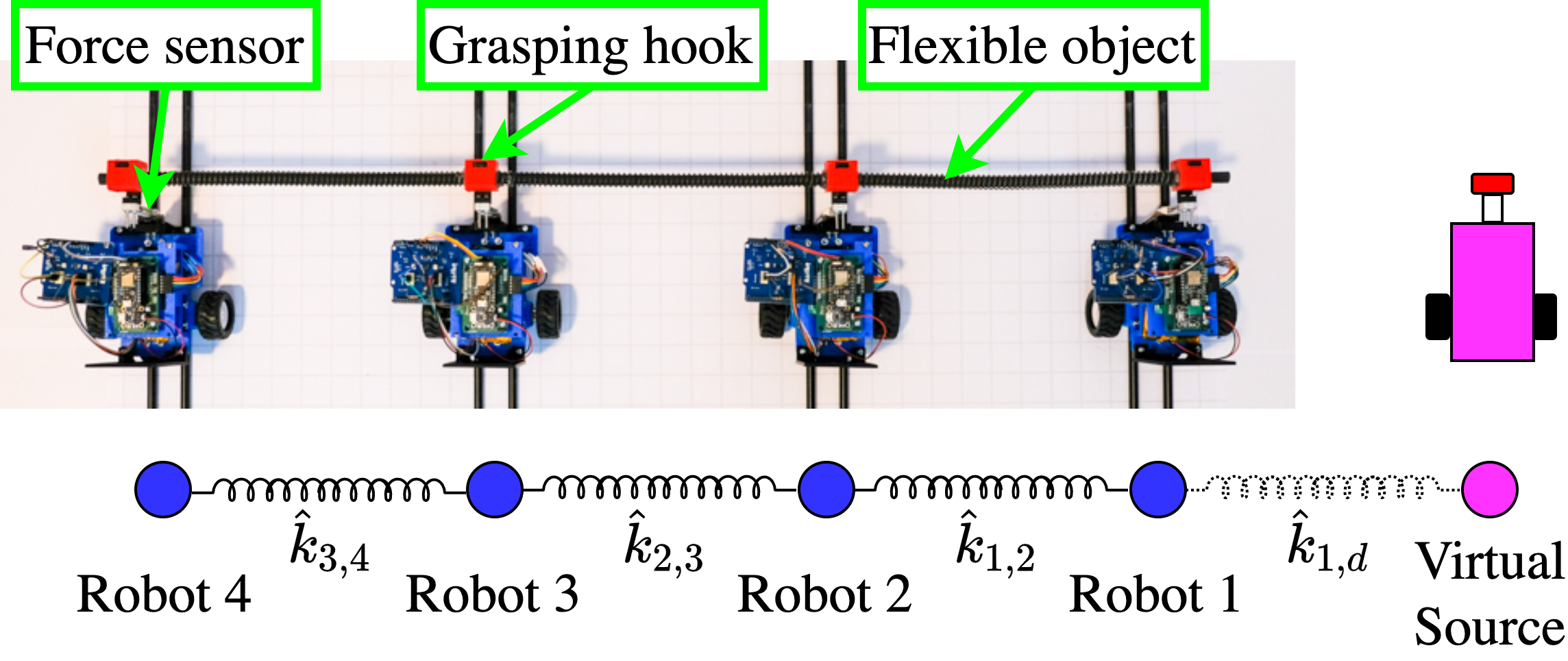
The robots are attached to a flexible object, e.g., as shown in Fig. 1. The position $y_{k}\in\mathbb{R}$ of each robot $k$ in the network is updated using local force measurements $f_{k}\in\mathbb{R}$ as well as a virtual force $\tilde{f}_{k}=\hat{k}_{k,d}(y_{k}-y_{d})\in\mathbb{R}$ if robot $k$ is a leader, as

	$\displaystyle y_{k}[m+1]$	$\displaystyle=y_{k}[m]-\gamma\hat{f}_{k}[m],$		(1)
	$\displaystyle\hat{f}_{k}[m]$	$\displaystyle=f_{k}[m]+\tilde{f}_{k}[m],$		(2)

where the update sampling-time period is $\delta_{t}$, $y_{k}[m]$ represents the position of robot $k$ at discrete time instants, e.g., $y_{k}[m]=y_{k}(m\delta_{t})$, $\gamma$ is the update gain, and the desired position from the virtual source $y_{d}\in\mathbb{R}$ is known (i.e., $\hat{k}_{k,d}\neq 0$) only if robot $k$ is a leader, e.g., $k=1$ in the example in Fig. 1. Each robot position $y_{k}$ is measured from an initial undeformed configuration (with all $y_{k}=0$) of the flexible object.

The local force-based robot position update in Eq. (1) achieves object transport, i.e., for a fixed desired position $y_{d}$, the network reaches equilibrium when each robot reaches the desired position, i.e., $y_{k}=y_{d}$ for all $k$ and the object has no distortion, i.e., $f_{k}=0$. To clarify, note that the local force $f_{k}$ measured by robot $k$ can be written linearly in terms of the position $y_{j}$ of all robots connected to robot $k$, provided the local deformation of the flexible object remains small, as

$$f_{k}[m]=\sum_{j=1}^{n}\hat{k}_{k,j}(y_{k}[m]-y_{j}[m]),$$

(3)

where $\hat{k}_{k,j}=\hat{k}_{j,k}\geq 0$ is the effective stiffness of the flexible object between two neighboring robots $j$ and $k$, $n$ is the number of robots, and $\hat{k}_{j,j}=0$ for all $1\leq j\leq n$. Then, the update law in Eq. (1) can be written in matrix form as

$\displaystyle\mathbf{Y}[m+1]$

$\displaystyle=(\mathbf{I}-\gamma\mathbf{K})\mathbf{Y}[m]+\gamma\mathbf{B}y_{d}[m],$

(4)

where $\mathbf{Y}=[y_{1},y_{2},\ldots,y_{k},\ldots,y_{n}]^{T}\in\mathbb{R}^{n}$ is the $n$ dimensional vector of the individual robots positions $y_{k}$, $B_{k}=\hat{k}_{k,d}$ is the $k^{th}$ element of $n$ dimensional vector $\mathbf{B}\in\mathbb{R}^{n}$ which is nonzero only if the robot $k$ is a leader and the symmetric matrix $\mathbf{K}$ is the pinned Laplacian with elements

$$\begin{array}[]{rcll}{\mathbf{K}}_{k,j}&=&\hat{k}_{k,d}+\sum_{m=1}^{n}\hat{k}_{k,m}~~\geq 0&{\mbox{if}}~k=j\\[3.00003pt] &=&-\hat{k}_{k,j}&{\mbox{otherwise}},\end{array}$$

(5)

with real nonzero eigenvalues $\lambda_{\mathbf{K},j}>0$ for $1\leq j\leq n$. It can be shown that for an update gain $\gamma$ satisfying

$$0<\gamma<\left(\overline{\gamma}~=2/\overline{\lambda}_{\mathbf{K}}~=2/\max_{j}(\lambda_{\mathbf{K},j})\right),$$

(6)

the eigenvalues of $(\mathbf{I}-\gamma\mathbf{K})$ are inside the unit circle. Therefore, the transport dynamics in Eq. (4) is stable, and the desired transport of the object can be achieved, i.e., for a fixed desired position $y_{d}$, the robot positions in $\mathbf{Y}$ converge to the desired value [19]

$$\lim_{m\rightarrow\infty}\mathbf{Y}[m]~=\textbf{1}_{n}y_{d}$$

(7)

with $\textbf{1}_{n}$ representing the $n$ dimensional vector of all ones.

The settling time $T_{s}$ to a new desired position $y_{d}$ can be selected by choosing the update gain $\gamma$. In particular, the settling time $T_{s}$ to reach and stay within 2% of a step change in the desired displacement $y_{d}$ can be estimated as

$$T_{s}\approx\frac{-4~\delta_{t}}{\ln\left(\lambda_{\mathbf{K}}^{*}\right)}~~{\mbox{where}}~\lambda_{\mathbf{K}}^{*}=\argmax_{\lambda_{\mathbf{K},j}}{|1-\gamma\lambda_{\mathbf{K},j}|}.$$

(8)

However, for a given settling time (i.e., given selection of the update gain $\gamma$), the deformations during transport can not be controlled further. Typically, faster settling (i.e., a smaller settling time $T_{s}$) also results in larger deformation. The research problem addressed here is to improve cohesion, i.e., to reduce the maximum deformation $\overline{D}$ of the object during transport,

$$\overline{D}=\max_{m}\left[D[m]=\max_{k,j}\big|\>(y_{j}[m]-y_{k}[m])\>\big|\right],$$

(9)

without increasing the settling time $T_{s}$.

The robot-position update to transport the object is chosen as a discrete-time approximation of an ideal cohesive network. For example, in the continuous time case, if each robot had access to the desired position $y_{d}$, i.e., in a centralized approach, then the ideal cohesive update can be written as,

$$\dot{\mathbf{Y}}(t)=-\alpha\mathbf{Y}(t)+\alpha\textbf{1}_{n}y_{d}(t),$$

(10)

where the gain $\alpha>0$ can be tuned to achieve a desired settling time and all robot move in a similar manner. The lack of access to centralized information about the desired position $y_{d}$ can be alleviated by multiplying both sides with the scaled pinned Laplacian $\beta\mathbf{K}$, substituting $\mathbf{K}\textbf{1}_{n}$ with $\mathbf{B}$  [18], and adding $\dot{\mathbf{Y}}$ to both sides and rearranging the equation to obtain

	$\displaystyle\dot{\mathbf{Y}}(t)$	$\displaystyle=-\alpha\beta\mathbf{KY}(t)+\alpha\beta\mathbf{B}y_{d}(t)+[\mathbf{I}-\beta\mathbf{K}]\dot{\mathbf{Y}}(t),$		(11)
		$\displaystyle\approx-\alpha\beta\mathbf{KY}(t)+\alpha\beta\mathbf{B}y_{d}(t)+\left[\mathbf{I}-\beta\mathbf{K}\right]\frac{\mathbf{Y}(t)-\mathbf{Y}(t-\tau)}{\tau}.$		(12)

With the time delay $\tau=\delta_{t}$ and the update kept constant between sampling periods, the update law in Eq. (12) for robot positions becomes

	$\displaystyle\mathbf{Y}[m+1]=$	$\displaystyle\mathbf{Y}[m]-\alpha\beta\delta_{t}\mathbf{KY}[m]+\alpha\beta\delta_{t}\mathbf{B}y_{d}[m]$		(13)
		$\displaystyle+\left[\mathbf{I}-\beta\mathbf{K}\right]\left(\mathbf{Y}[m]-\mathbf{Y}[m-1]\right).$

Then for each robot $k$, the update law becomes

	$\displaystyle y_{k}[m+1]=$	$\displaystyle y_{k}[m]-\alpha\beta\delta_{t}f_{k}[m]+\alpha\beta\delta_{t}\hat{k}_{k,d}\big(y_{d}[m]-y_{k}[m]\big)$
		$\displaystyle{+(1-\beta\hat{k}_{k,d})\big(y_{k}[m]-y_{k}[m-1]\big)}$
		$\displaystyle-\beta\big(f_{k}[m]-f_{k}[m-1]\big).$		(14)

Note that this cohesive transport law is decentralized. For each robot, in addition to the virtual source position $y_{d}$ if the robot is a leader, the update only requires current information and delayed self reinforcement (DSR) by a time step of: (i) local force measurements $f_{k}$ and (ii) its own position $y_{k}$.

Stability conditions can be established by finding the roots of the characteristic equation of the cohesive dynamics in Eq. (13), i.e.,

$\displaystyle\det\Big(\mathbf{I}z^{2}-\left(\mathbf{I}-\alpha\beta\delta_{t}\mathbf{K}_{J}+[\mathbf{I}-\beta\mathbf{K}_{J}]\right)z+[\mathbf{I}-\beta\mathbf{K}_{J}]\Big)=0,$

(15)

where $\mathbf{K}_{J}=\mathbf{P_{K}}^{-1}\mathbf{KP_{K}}$ is the diagonalization of the pinned Laplacian $\mathbf{K}$ with eigenvalues $\lambda_{\mathbf{K},k}$ along the diagonal. In particular, the cohesive dynamics in Eq. (13) is stable if and only if, for each eigenvalue $\lambda_{\mathbf{K},k}$ of the pinned Laplacian $\mathbf{K}$, the roots of $D(z)$ where

	$\displaystyle D(z)=$	$\displaystyle z^{2}-\left(1-\alpha\beta\delta_{t}\lambda_{\mathbf{K},k}+[1-\beta\lambda_{\mathbf{K},k}]\right)z$		(16)
		$\displaystyle+[1-\beta\lambda_{\mathbf{K},k}]=0$

have magnitude less than one. Thus, stability can be evaluated by computing the roots of Eq. (16). Nevertheless, for design purposes, it is preferable to establish analytical conditions on the DSR parameters for stability, as shown next.

To easily visualize the deformation during transport, a highly flexible object (a long spring coiled with diameter of $1.30\;cm$ and length of $90\;cm$) was selected for transport using a robot network as shown in Fig. 1. Only the leader (robot 1) has knowledge of the desired position illustrated by the virtual source shown in pink in Fig. 1. Each robot $k$ measures the local force $f_{k}$ using a force sensor between the robot and the object, and senses its position $y_{k}$ using magnetic encoders on the wheels, and uses an on-board micro-controller to compute the next position $y_{k}[m+1]$. The updated position $y_{k}[m+1]$ is achieved within the sampling-time period $\delta_{t}=0.03\;s$, using a velocity feedback control to maintain the velocity at $v_{d,k}(t)=(y_{k}[m+1]-y_{k}[m])/\delta_{t}$ as shown in Fig. 2.

The system dynamics in Eq. (1) was found by estimating the elastic object stiffness $\hat{k}_{i,j}$ experimentally. In particular, for estimating $\hat{k}_{1,2}$, robot 1 was moved for a known distance $y_{1}$ without moving the other robots (nor connecting robot 1 to the virtual source) and the resulting force $f_{1}$ was measured to yield $\hat{k}_{1,2}=f_{1}/y_{1}$. Then, to estimate stiffness $\hat{k}_{2,3}$, robot 2 was moved for a known distance $y_{2}$ without moving the other robots and the resulting force $f_{2}$ was measured to yield $\hat{k}_{2,3}=(f_{2}/y_{2})-\hat{k}_{1,2}$. The same procedure is used to obtain the rest of the effective stiffness coefficients, which are all the same and given by $\hat{k}_{i,i+1}=0.05\;N/cm,\;{\mbox{for}}\;1\leq i\leq 3,$ which is to be expected since the connecting springs have similar lengths. For the setup shown in Fig. 1, the stiffness of the connection with virtual source is chosen to be same as the other spring elements, i.e., $\hat{k}_{1,d}=0.05$. The resulting pinned Laplacian $\mathbf{K}$ and matrix $\mathbf{B}$ were

	$\displaystyle\mathbf{K}$	$\displaystyle=\begin{bmatrix}\hat{k}_{1,2}+\hat{k}_{1,d}&-\hat{k}_{1,2}&0&0\\ -\hat{k}_{1,2}&\hat{k}_{1,2}+\hat{k}_{2,3}&-\hat{k}_{2,3}&0\\ 0&-\hat{k}_{2,3}&\hat{k}_{2,3}+\hat{k}_{3,4}&-\hat{k}_{3,4}\\ 0&0&-\hat{k}_{3,4}&\hat{k}_{3,4}\end{bmatrix}$
		$\displaystyle=\begin{bmatrix}0.10&-0.05&0&0\\ -0.05&0.10&-0.05&0\\ 0&-0.05&0.10&0.05\\ 0&0&-0.05&0.05\end{bmatrix},$		(18)
	$\displaystyle\mathbf{B}$	$\displaystyle=\begin{bmatrix}\hat{k}_{1,d}&0&0&0\end{bmatrix}^{T}~=\begin{bmatrix}0.05&0&0&0\end{bmatrix}^{T}.$		(19)

To avoid optimization over each desired trajectory $y_{d}$, the control parameters are selected to minimize the deformation for a specified settling time $T_{s}$ for a unit step change in the desired position $y_{d}$.

A large change in position $y_{d}$ from $0\;cm$ to $50\;cm$ was chosen to help visualize the transport of the flexible body. To ensure that the deformations are not too large (i.e., to avoid other robots dragging each other), the desired transport trajectory $y_{d}$ was chosen as a step that is filtered using a first-order, low-pass filter with cutoff frequency $\omega_{c}$ and implemented using Tustin’s approximation, as

$$y_{d}[m]=\frac{2-\omega_{c}\delta_{t}}{2+\omega_{c}\delta_{t}}y_{d}[m-1]+\frac{\omega_{c}\delta_{t}}{2+\omega_{c}\delta_{t}}\left(y_{ds}[m]+y_{ds}[m-1]\right),$$

(22)

where $y_{ds}[m]=50$ if $m>0$ and zero otherwise. The effect of the cutoff frequency $\omega_{c}$ on maximum deformation $\overline{D}$ in Eq. (9) is shown in Fig. 6a. The cutoff frequency $\omega_{c}$ was selected as $\omega_{c}=0.1\;rad/s$ so that the maximum deformation $\overline{D}$ is below $7\;cm$ and the maximum speed input to the robot $v_{d,k}\leq(v_{max}=5\;cm/s)$ to avoid dragging of the robots by each other for the case without DSR. Note that the desired trajectory $y_{d}$ reaches the final value of $50\;cm$ in about $T_{sf}=4/\omega_{c}=40\;s$ as seen in Fig. 6b.

Comparative evaluations, with and without the DSR approach, are presented below. The results are evaluated based on the maximum deformation $\overline{D}$ in Eq. (9) and also the maximum force $\overline{f}$ defined as

$$\overline{f}=\max_{k=\{1,2,3,4\}}\left(\max_{m}|f_{k}[m]|\right).$$

(23)

The simulation and experimental results are shown in Fig. 5, and quantified in Table  I. The responses from the experiments and simulations are similar to each other in Fig. 5, which indicates that the models are close to the experimental system. The cohesive DSR approach reduces the maximum deformation $\overline{D}$ substantially, by $90\%$ in simulation and $85\pm 0.05\%$ in experiment. Similarly, the corresponding maximum forces $\overline{f}$ are also reduced significantly, by $90\%$ in simulation and $87\pm 0.50\%$ in experiment. The reduction in deformation indicates that the robot network responses are more cohesive during transport with the cohesive DSR approach. This increased cohesion can also be observed from snapshots of experiment in Fig. 7.

References

- [1] Y. E. Nesterov, “A Method of Solving a Convex Programming Problem with Convergence Rate of ,” Soviet Mathematics Doklady, vol. 27, no. 3, pp. 372–376, 1983.
- [2] B. Van Scoy, R. A. Freeman, and K. M. Lynch, “The fastest known globally convergent first-order method for minimizing strongly convex functions,” IEEE Control Systems Letters, vol. 2, no. 1, pp. 49–54, Jan 2018.
- [3] Kar-Han Tan and M. A. Lewis, “Virtual structures for high-precision cooperative mobile robotic control,” in Proceedings of IEEE/RSJ International Conference on Intelligent Robots and Systems. IROS ’96, vol. 1, Nov 1996, pp. 132–139 vol.1.
- [4] B. Khoshnevis and G. Bekey, “Centralized sensing and control of multiple mobile robots,” Computers and Industrial Engineering, vol. 35, no. 3, pp. 503 – 506, 1998, selected Papers from the 22nd ICC and IE Conference. [Online]. Available: http://www.sciencedirect.com/science/article/pii/S0360835298001442
- [5] A. Petitti, A. Franchi, D. Di Paola, and A. Rizzo, “Decentralized motion control for cooperative manipulation with a team of networked mobile manipulators,” in 2016 IEEE International Conference on Robotics and Automation (ICRA), May 2016, pp. 441–446.
- [6] A. Tsiamis, C. K. Verginis, C. P. Bechlioulis, and K. J. Kyriakopoulos, “Cooperative manipulation exploiting only implicit communication,” in 2015 IEEE/RSJ International Conference on Intelligent Robots and Systems (IROS), Sep. 2015, pp. 864–869.
- [7] Z. Wang and M. Schwager, “Kinematic multi-robot manipulation with no communication using force feedback,” in 2016 IEEE International Conference on Robotics and Automation (ICRA), May 2016, pp. 427–432.
- [8] B. E. Jackson, T. A. Howell, K. Shah, M. Schwager, and Z. Manchester, “Scalable Cooperative Transport of Cable-Suspended Loads With UAVs Using Distributed Trajectory Optimization,” IEEE Robot. Autom. Lett., vol. 5, no. 2, pp. 3368–3374, Apr. 2020. [Online]. Available: https://ieeexplore.ieee.org/document/9007450/
- [9] Jianing Chen, M. Gauci, Wei Li, A. Kolling, and R. Gros, “Occlusion-Based Cooperative Transport with a Swarm of Miniature Mobile Robots,” IEEE Trans. Robot., vol. 31, no. 2, pp. 307–321, Apr. 2015. [Online]. Available: http://ieeexplore.ieee.org/document/7055285/
- [10] G. Montemayor and J. T. Wen, “Decentralized collaborative load transport by multiple robots,” in Proceedings of the 2005 IEEE International Conference on Robotics and Automation, April 2005, pp. 372–377.
- [11] A. Gelblum, I. Pinkoviezky, E. Fonio, A. Ghosh, N. Gov, and O. Feinerman, “Ant groups optimally amplify the effect of transiently informed individuals,” Nature Communications, vol. 6, no. 1, p. 7729, 2015. [Online]. Available: https://doi.org/10.1038/ncomms8729
- [12] H. Bai and J. T. Wen, “Cooperative load transport: A formation-control perspective,” IEEE Transactions on Robotics, vol. 26, no. 4, pp. 742–750, Aug 2010.
- [13] G. Loianno and V. Kumar, “Cooperative Transportation Using Small Quadrotors Using Monocular Vision and Inertial Sensing,” IEEE Robot. Autom. Lett., vol. 3, no. 2, pp. 680–687, Apr. 2018. [Online]. Available: http://ieeexplore.ieee.org/document/8120115/
- [14] S. Thapa, R. V. Self, R. Kamalapurkar, and H. Bai, “Cooperative manipulation of an unknown payload with concurrent mass and drag force estimation,” IEEE Control Systems Letters, vol. 3, no. 4, pp. 907–912, Oct 2019.
- [15] J. Alonso-Mora, R. Knepper, R. Siegwart, and D. Rus, “Local motion planning for collaborative multi-robot manipulation of deformable objects,” in 2015 IEEE International Conference on Robotics and Automation (ICRA), May 2015, pp. 5495–5502.
- [16] S. Flixeder, T. Glück, and A. Kugi, “Modeling and Force Control for the Collaborative Manipulation of Deformable Strip-Like Materials,” IFAC-PapersOnLine, vol. 49, no. 21, pp. 95–102, 2016. [Online]. Available: https://linkinghub.elsevier.com/retrieve/pii/S2405896316321085
- [17] E. Rossi, M. Tognon, R. Carli, L. Schenato, J. Cortes, and A. Franchi, “Cooperative Aerial Load Transportation via Sampled Communication,” IEEE Control Syst. Lett., vol. 4, no. 2, pp. 277–282, Apr. 2020.
- [18] S. Devasia, “Cohesive networks using delayed self reinforcement,” Automatica, vol. 112, p. 108699, 2020. [Online]. Available: http://www.sciencedirect.com/science/article/pii/S000510981930562X
- [19] R. Olfati-Saber, J. Fax, and R. Murray, “Consensus and cooperation in networked multi-agent systems,” Proceedings of the IEEE, vol. 95, no. 1, pp. 215–233, Jan 2007.