Estimating The Proportion of Signal Variables Under
Arbitrary Covariance Dependence

Meinshausen and Rice 2006 introduced a family of proportion estimators that are built upon the empirical process of $p$-values under independence. This family of estimators have been proved to provide lower bound estimates for the true proportion $\pi$. Members in the family are indexed by the choice of a bounding function, and it has been shown that the estimator with bounding function $\delta(u)=\sqrt{u(1-u)}$ has the best overall performance for signals of different sparsity levels. This conclusion, unfortunately, does not hold anymore under arbitrary dependence. When variables are arbitrarily dependent, the limiting distribution of the empirical process of $p$-values is generally unknown and may not even have an analytic expression. Moreover, the dependence effect mingles with signal sparsity to influence the performances of different estimators in the family. These difficulties substantially complicate the estimation problem and motivate us to develop new techniques to study the family of estimators and to come up with a new powerful estimator under arbitrary covariance dependence.

For presentation simplicity, we perform inverse normal transformation as $Z_{j}=\Phi^{-1}(F_{0}(X_{j}))$, where $\Phi^{-1}$ is the inverse of the cumulative distribution function of a standard Normal distribution. Then, we have

where $G$ denotes the signal distribution after inverse normal transformation, which remains unknown.

Next, we construct a modified family of estimators to accommodate dependence among $Z_{j}$. Let

where $(W_{1},\ldots,W_{p})$ follow the joint null distribution of $(Z_{1},\ldots,Z_{p})$. Denote $\bar{\Phi}(t)=1-\Phi(t)$. For a given function $\delta(t)$ that is strictly positive on $(0,\infty)$, define

Apparently, $V_{p,\delta}$ varies with the choice of $\delta(t)$, and $\delta(t)$ is called a bounding function. For a given $\delta(t)$ and a control level $\alpha$, we define the corresponding bounding sequence $c_{p,\delta}$ as a function of $p,\delta$ and $\alpha$ that satisfies the following properties:

(a) $pc_{p,\delta}>p_{0}c_{p_{0},\delta}$, where $p_{0}=|I_{0}|$, and

(b) $P(V_{p,\delta}>c_{p,\delta})<\alpha$ for all $p$.
From the above properties, it can be seen that $c_{p,\delta}$ is an upper bound of $V_{p,\delta}$, while $V_{p,\delta}$ relies on the joint null distribution. Both $V_{p,\delta}$ and $c_{p,\delta}$ carry the information of dependence among the variables. Also, the absolute sign in the numerator of (2) stabilizes $V_{p,\delta}$ as $\bar{W}_{p}(t)-2\bar{\Phi}(t)$ may not be asymptotically symmetric anymore under arbitrary dependence.

Then, given the observed $Z_{j}$, a family of estimators indexed by $\delta$ are constructed as

where

It can be seen that the $\hat{\pi}_{\delta}$ family of estimators hinge on the choices of the bounding function $\delta(t)$ and the corresponding bounding sequence $c_{p,\delta}$. As the bounding sequence $c_{p,\delta}$ implies a normal range of $\bar{F}_{p}(u)$ if all variables are noise, the information carried by the observed $\bar{F}_{p}(u)$ that exceeds the normal range presents evidence for the existence of signals. This version of lower bound family is for signals of two-sided effects. Minor changes to accommodate one-sided signal effect is straightforward. Details for the numerical implementation of $\hat{\pi}_{\delta}$ can be found at the end of Section 2.3.

As shown in Meinshausen and Rice 2006, for signals of different sparsity levels, the performances of the estimators in the original family can be very different under independence. More specifically, the signal proportion can be re-parameterized as $\pi=p^{-\gamma}$, $\gamma\in(0,1)$, with $\gamma\in(0,1/2)$ representing the relatively dense case and $\gamma\in[1/2,1)$ representing the more sparse case. Consistency of different estimators in the original family was proved under independence for $\gamma\in(0,1/2)$ and $\gamma\in[1/2,1)$ separately. Here, we consider the estimation problem in the more challenging setting with arbitrary dependence and the modified family of estimators to accommodate the dependence.

First, we impose a monotonicity constraint on the bounding function $\delta(t)$, which allows us to present the following result under general dependence for signals of sparsity levels in the full range of $\gamma\in(0,1)$.

The above theorem says that the lower bound property of $\hat{\pi}_{\delta}$ in (4) holds as long as a bounding sequence $c_{p,\delta}$ satisfying (a) and (b) can be found. On the other hand, the upper bound property of $\hat{\pi}_{\delta}$ in (5) holds under certain conditions on the signal distribution $G$, which essentially says that the signal effect, either positive ($G<\Phi$) or negative ($G>\Phi$), is strong enough. When both lower bound and upper bound conditions are satisfied for a given $\delta(t)$ and a degenerating $\alpha$ such that $\alpha=\alpha_{p}\to 0$, $\hat{\pi}_{\delta}$ consistently estimate the true signal proportion, i.e., for any constant $\epsilon>0$,

The above results hold for arbitrarily dependent variables and for sparse signals that are not of a fixed proportion of all the variables. Such sparsity condition covers the full range of $\gamma\in(0,1)$.

As individual estimators in the $\hat{\pi}_{\delta}$ family hinge on the choice of the bounding function, we further study their consistency with specific $\delta(t)$ functions. We focus on $\delta(t)$ of the form $\delta(t)=[\bar{\Phi}(t)]^{\theta}$, $\theta\in[0,1]$, so that the corresponding $\hat{\pi}_{\delta}$ are closely related to several existing estimators whose consistency has been studied under independence in literature (please see Meinshausen and Rice 2006 and the references therein). Valuable insight can be obtained by comparing the estimators’ performances under independence and dependence, which helps us construct a new and more powerful estimator under arbitrary covariance dependence.

In order to explicate the effect of dependence on $\hat{\pi}_{\delta}$, we assume that

where $\mu$ is a $p$-dimensional sparse vector with $\mu_{j}=A\cdot 1\{j\in I_{1}\}$, $A\neq 0$, and $\Sigma$ is an arbitrary correlation matrix, i.e., $\Sigma_{ij}=Corr(Z_{i},Z_{j})$. For presentation simplicity, assume $A>0$. We define the Mean Absolute Correlation (MAC) to calibrate the covariance dependence as

A larger value of $\bar{\rho}_{\Sigma}$ indicates stronger overall dependence.

Moreover, we employ a discretization technique from Arias-Castro et al. 2011 and Jeng and Chen 2019 as follows. Define $\mathbb{T}=[1,\sqrt{5\log p}]\cap\mathbb{N}$ and the discretized version of $V_{p,\delta}$ as

Denote $c^{*}_{p,\delta}$ as the bounding sequence based on $V^{*}_{p,\delta}$, and define the corresponding proportion estimator as

Next, we explicates how the MAC level interacts with signal sparsity and signal intensity to influence the consistency of $\hat{\pi}^{*}_{\delta}$ with $\delta(t)=[\bar{\Phi}(t)]^{\theta}$ and reveals very different results for $\theta\in[0,1/2]$ and $\theta\in(1/2,1]$.

The above theorem says that for $\delta(t)=[\bar{\Phi}(t)]^{\theta}$ with $\theta\in[0,1/2]$, we can find a bounding sequence $c_{p,\delta}^{*}$, whose order increases with respect to $\bar{\rho}_{\Sigma},p$ and $\theta$, respectively. The second part of the theorem provides a condition on the signal distribution for the consistency of $\hat{\pi}^{*}_{\delta}$. This condition is easier to be satisfied for less sparse signals (larger $\pi$) or less dependent variables (smaller $\bar{\rho}_{\Sigma}$). Note that $\bar{\Phi}^{-1}(\pi^{1/\theta}/(\bar{\rho}_{\Sigma}^{1/(2\theta)}(\log p)^{(\theta+1/2)/(2\theta)}))$ is well-defined only for $\pi<\sqrt{\bar{\rho}_{\Sigma}(\log p)^{\theta+1/2}}$. In the case $\pi\geq\sqrt{\bar{\rho}_{\Sigma}(\log p)^{\theta+1/2}}$, condition on $A_{p}$ is simply $A_{p}\gg 1$. For the special case with independent variables, $\bar{\rho}_{\Sigma}=1/p$ and(10) degenerates to

which agrees with the sufficient and necessary condition for the consistency of $\hat{\pi}_{\delta}$ under independence for relatively sparse signals. The comparison can be made by adopting the same parameterization as in Theorem 3 of Meinshausen and Rice 2006 with $\pi=p^{-\gamma}$, $\gamma\in[1/2,1)$, $\nu=\theta$, and $\kappa=2$.

Results in Theorem 2.2 explicate how the performance of $\hat{\pi}^{*}_{\delta}$ with $\delta(t)=[\bar{\Phi}(t)]^{\theta},\theta\in[0,1/2]$ deteriorates as the MAC dependence gets stronger. These results, however, cannot be extended to $\hat{\pi}^{*}_{\delta}$ with $\theta\in(1/2,1]$. For the latter, we present the following theorem.

This theorem shows that for $\delta(t)=[\bar{\Phi}(t)]^{\theta}$ with $\theta\in(1/2,1]$, we can find a bounding sequence $c_{p,\delta}^{*}$, whose order does not involve the MAC dependence level $\bar{\rho}_{\Sigma}$. Moreover, the intensity condition in (11) does not involve $\bar{\rho}_{\Sigma}$, which means that $\hat{\pi}^{*}_{\delta}$ with $\theta\in(1/2,1]$ is consistent under (11), no matter how strong the MAC dependence is.

Although the above analyses are for the discretized version of $\hat{\pi}_{\delta}$, they provides important insight on the performance of the $\hat{\pi}_{\delta}$ family under dependence, which is also supported by extensive simulation studies in Section 3.

Study in the previous section reveals very different effects of the MAC dependence on different estimators in the $\hat{\pi}_{\delta}$ family. When MAC dependence is relatively weak, estimators with $\theta\in[0,1/2]$ may be more powerful as condition (10) is less restrictive for smaller $\bar{\rho}_{\Sigma}$. On the other hand, when MAC dependence gets stronger, estimators with $\theta\in(1/2,1]$ could be more powerful as condition (11) is free of $\bar{\rho}_{\Sigma}$. Motivated by these findings, we propose to construct a new estimator of the form

where $\Delta$ is the set of $\delta(t)$ functions that render the most powerful estimators in different dependence scenarios. Note that such $\delta(t)$ functions in $\Delta$ all result in conservative estimators with the lower bound property as stated in Theorem 2.1. Therefore, the new estimator $\hat{\pi}_{adap}$ naturally inherit the lower bound property.

The power of $\hat{\pi}_{adap}$ depends on the candidate $\delta(t)$ functions in $\Delta$. We consider $\delta(t)=[\bar{\Phi}(t)]^{\theta}$ with specific $\theta$ values. Informed by Theorem 2.2, which is for all the estimators with $\theta\in[0,1/2]$, we see that condition (10) is less stringent with larger $\theta$. Therefore, we expect the estimator with $\theta=1/2$ to be the most powerful candidate in this group. On the other hand, based on the results in Theorem 2.3, we expect the most powerful estimator in the group of estimators with $\theta\in(1/2,1]$ to have $\theta=1$. The above analysis helps us narrow down to two candidates that are most powerful in their own $\theta$ groups. Comparing these two candidates, we see that $\theta=1/2$ can result in a more (or less) powerful estimator than $\theta=1$ when MAC dependence is relatively weak (or strong) with $\bar{\rho}_{\Sigma}\leq\pi/\sqrt{\log p}$ (or $\bar{\rho}_{\Sigma}>\pi/\sqrt{\log p}$). Since none of the candidates dominates the other under arbitrary covariance dependence, our new estimator is constructed as

where $\hat{\pi}_{0.5}$ denotes $\hat{\pi}_{\delta}$ with $\delta=[\bar{\Phi}(t)]^{1/2}$, and $\hat{\pi}_{1}$ denotes $\hat{\pi}_{\delta}$ with $\delta=\bar{\Phi}(t)$. $\hat{\pi}_{adap}$ is likely to be comparable to $\hat{\pi}_{0.5}$ and outperform $\hat{\pi}_{1}$ under relatively weak dependence, and be comparable to $\hat{\pi}_{1}$ and outperform $\hat{\pi}_{0.5}$ when covariance dependence is strong.

Numerical Implementation. We conclude this section with additional notes on the numerical implementation of $\hat{\pi}_{adap}$. Specifically, we simulate $(w_{1},\ldots,w_{p})$ following the joint null distribution of $Z_{j}$. When the joint null distribution is unknown in real applications, $(w_{1},\ldots,w_{p})$ can often be simulated non-parametrically. For example, when $(Z_{1},\ldots,Z_{p})$ are a set of test statistics for associations between a set of explanatory variables and a response variable, a common practice to simulate $(w_{1},\ldots,w_{p})$ is by randomly shuffling only the sample of the response variable to remove the potential associations. More details for such permutation approaches can be found in Westfall and Young 1993. Then, following (2), we simulate $V_{p,0.5}$ and $V_{p,1}$ corresponding to $\theta=1/2$ and $1$ by taking the maximums over $t=w_{1},\ldots,w_{p}$. Next, we set $\alpha=0.1$ and generate $c_{p,0.5}$ and $c_{p,1}$ as the $(1-\alpha)$th quantile of 1000 replicates of $V_{p,0.5}$ and $V_{p,1}$, respectively. The simulated $c_{p,0.5}$ and $c_{p,1}$ are implemented to calculate $\hat{\pi}_{0.5}$ and $\hat{\pi}_{1}$ as in (3) by taking the maximums over $t=z_{1},\ldots z_{p}$, where $z_{1},\ldots z_{p}$ are the observed variables after inverse normal transformation. Finally, the new estimator $\hat{\pi}_{adap}$ is calculated by (12).

We first calculate the MAC levels as defined in (7) for the dependence structures in (a)-(f) above and report the realized values of $c_{p,0.5}$ and $c_{p,1}$, which are generated by the procedure described at the end of Section 2.3. Recall that a larger value of $\bar{\rho}_{\Sigma}$ indicates stronger overall covariance dependence. It can be seen in Table 1 that $\bar{\rho}_{\Sigma}$ is fairly small for cases (a) and (d), moderately small for cases (c) and (e), and fairly large for cases (b) and (f). Moreover, $c_{p,0.5}$ seems to vary positively with $\bar{\rho}_{\Sigma}$, whereas $c_{p,1}$ does not show such tendency. The numerical results are demonstrated more clearly in Figure 1, which seem to agree with the theoretical results in Theorem 2.2 and 2.3 about the MAC dependence effect on $c_{p,0.5}$ and $c_{p,1}$.

We compare the new estimator $\hat{\pi}_{adap}$ with $\hat{\pi}_{0.5}$ and $\hat{\pi}_{1}$ from the estimator family as well as two other popular methods. Note that $\hat{\pi}_{0.5}$ is closely related to the optimal estimator in the original family of Meinshausen and Rice 2006 under independence, and $\hat{\pi}_{1}$ has been discovered to have good power for relatively sparse signals under independence. The two other existing methods are $\hat{\pi}_{GW}$ developed in Genovese and Wasserman 2004 and $\hat{\pi}_{JC}$ developed in Jin and Cai 2007b. These two existing methods have been studied for relatively dense signals under independence.

Besides various dependence structures in (a)-(f), we consider sparse and relatively dense signals with $\pi=0.02$ and $0.1$, respectively, and varying signal intensity with non-zero $\mu_{j}=3,4,5,6$. The comparisons are organized into two sets of examples.

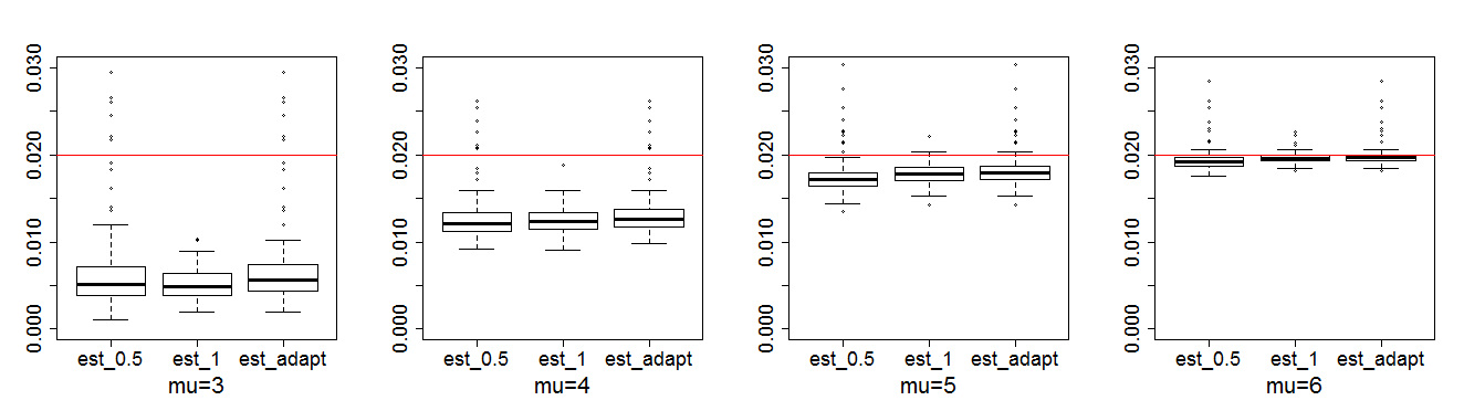
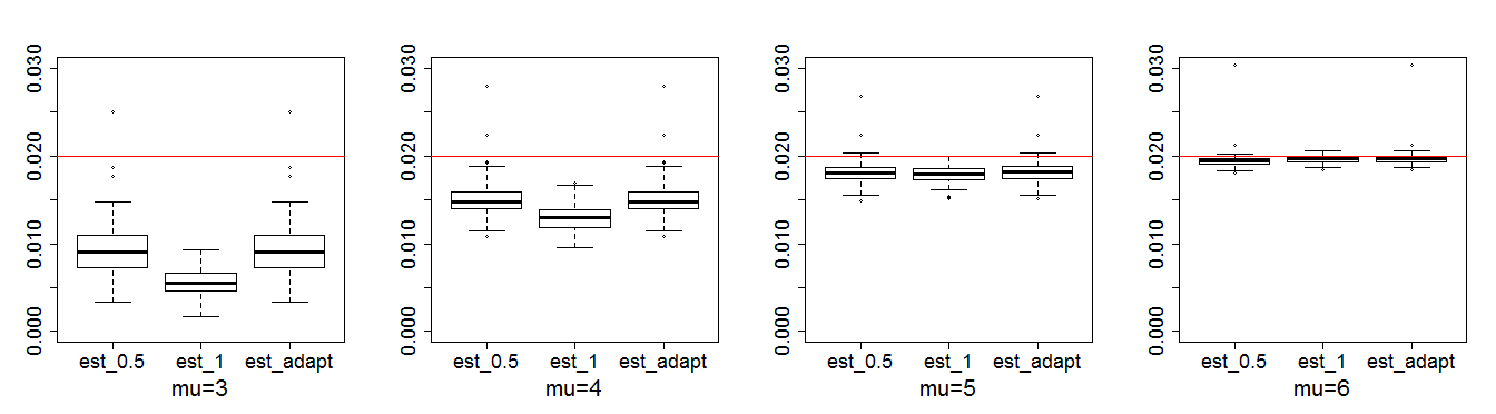
The first set of examples demonstrate the performances of $\hat{\pi}_{adap}$, $\hat{\pi}_{0.5}$, and $\hat{\pi}_{1}$ as they all possess the lower bound property. Recall the theoretical results in Section 2.2 that $\hat{\pi}_{0.5}$ may outperform $\hat{\pi}_{1}$ when dependence is weak enough or signals are less sparse, and $\hat{\pi}_{1}$ may perform better in the other scenarios. We observe such tendencies in Figure 2-7. Specifically, the autocorrelation case (Figure 2) has small $\bar{\rho}_{\Sigma}=0.0095$. It shows that $\hat{\pi}_{0.5}$ has comparable results as those of $\hat{\pi}_{1}$ for small $\pi=0.02$, and outperforms $\hat{\pi}_{1}$ for larger $\pi=0.1$. The equal correlation case (Figure 3) has the largest $\bar{\rho}_{\Sigma}=0.5$. It shows that $\hat{\pi}_{1}$ outperforms $\hat{\pi}_{0.5}$ for both $\pi=0.02$ and $0.1$. The block diagonal case (Figure 4) has moderate $\bar{\rho}_{\Sigma}=0.1$. It shows that $\hat{\pi}_{1}$ outperforms $\hat{\pi}_{0.5}$ for small $\pi$, and is comparable to $\hat{\pi}_{0.5}$ for larger $\pi$. The sparse correlation case (Figure 5) has the smallest $\bar{\rho}_{\Sigma}=0.0042$, we see that $\hat{\pi}_{0.5}$ outperforms $\hat{\pi}_{1}$ for both $\pi=0.02$ and $0.1$. The SNP correlation case (Figure 6) has $\bar{\rho}_{\Sigma}=0.0869$, which is moderately small. We see that $\hat{\pi}_{1}$ is slightly better for small $\pi$, and $\hat{\pi}_{0.5}$ is better for larger $\pi$. The gene correlation case (Figure 7) has $\bar{\rho}_{\Sigma}=0.3353$, which is fairly large. It shows that $\hat{\pi}_{1}$ outperforms $\hat{\pi}_{0.5}$ for both small and larger $\pi$. In all these examples, the new estimator $\hat{\pi}_{adap}$ always matches the winner of $\hat{\pi}_{0.5}$ and $\hat{\pi}_{1}$ and exhibits better adaptivity to different dependence structures and signal sparsity levels.

The second set of examples compares the performance of $\hat{\pi}_{adap}$ with those of $\hat{\pi}_{GW}$ from Genovese and Wasserman 2004 and $\hat{\pi}_{JC}$ from Jin and Cai 2007b. Table 2 and 3 show that for the cases (a)-(f), $\hat{\pi}_{GW}$ and $\hat{\pi}_{JC}$ tend to over-estimate the true $\pi$ when dependence is strong (such as in (b) Equal correlation and (f) Gene correlation) or signals are sparse (such as for $\pi=0.02$). On the other hand, the performance of $\hat{\pi}_{adap}$ seems to be generally more accurate and stable over different dependence structures and $\pi$ values.

We first show $P(\hat{\pi}_{\delta}<\pi)\geq 1-\alpha$. Let $Z_{j}^{0}=Z_{j}$ for $j\in I_{0}$ and $Z_{j}^{1}=Z_{j}$ for $j\in I_{1}$. Denote $p_{0}=|I_{0}|$ and $s=|I_{1}|$. Then

Consequently,

where the second and last inequalities are by properties (a) and (b) of $c_{p,\delta}$, respectively. The claim $P(\hat{\pi}_{\delta}<\pi)\geq 1-\alpha$ follows.

Next, we show $P(\hat{\pi}_{\delta}>(1-\epsilon)\pi)\to 1$. Because $\hat{\pi}_{\delta}>\bar{F}_{p}(t)-2\bar{\Phi}(t)-c_{p,\delta}\delta\left(t\right)$ for any $t>0$ and

then

for any $t>0$. Now, set $t$ in (13) at $\tau$ such that $\tau\gg 1$ and $\delta(\tau)\ll\pi/c_{p,\delta}$. We will show that each term on the right hand side of (13) at $t=\tau$ is of $o_{p}(1)$.

First, by the condition $\delta(\tau)\ll\pi/c_{p,\delta}$, we have the first term $A_{1}=-c_{p,\delta}\delta(\tau)/\pi=o(1)$.

Consider the second term $A_{2}=\pi^{-1}(1-\pi)\left(p_{0}^{-1}\sum\nolimits_{j\in I_{0}}1_{\{|Z_{j}^{0}|>\tau\}}-2\bar{\Phi}(\tau)\right)$ in (13). The following lemma is proved in Section 5.2.

Lemma 5.1and the condition $\pi=o(1)$ are enough to show $A_{2}=o_{p}(1)$.

For the third term $A_{3}={s}^{-1}\sum\nolimits_{j\in I_{1}}1_{\{|Z_{j}^{1}|>\tau\}}-1$ in (13), we have

for any fixed $a>0$, where the third step is by $Z_{j}^{1}\sim G$ for $j\in I_{1}$, and the last the step is by the condition $G(\tau)\to 0$ or $G(-\tau)\to 1$.

Last but not least, the forth term in (13): $A_{4}=-2\bar{\Phi}(\tau)=o(1)$ given $\tau\gg 1$.

Summarizing the above gives the desired result $P(\hat{\pi}_{\delta}/\pi>1-\epsilon)\to 1$.

Recall the definitions of $V_{p,\delta}$ in (2) and

where $W_{1},\ldots,W_{p}\sim N_{p}(0,\Sigma)$. Then, for $t=\tau$,

Given $c_{p,\delta}\delta(\tau)/\pi=o(1)$, we have

Decompose the left hand side above as

References

- Arias-Castro et al. (2011) Arias-Castro, E., E. J. Candès, and Y. Plan (2011). Global testing under sparse alternatives: Anova, multiple comparisons and the higher criticism. The Annals of Statistics 39(5), 2533–2556.
- Bradic et al. (2011) Bradic, J., J. Fan, and W. Wang (2011). Penalized composite quasi-likelihood for ultrahigh dimensional variable selection. Journal of the Royal Statistical Society: Series B 73(3), 325–349.
- Buhlmann et al. (2014) Buhlmann, P., K. Kalisch, and L. Meier (2014). High-dimensional statistics with a view toward applications in biology. Annu Rev Stat Appl. 1, 255–278.
- Cai et al. (2013) Cai, T., W. Liu, and Y. Xia (2013). Two-sample covariance matrix testing and support recovery in high-dimensional and sparse settings. Journal of the American Statistical Association 108(501), 265–277.
- Cai and Sun (2017) Cai, T. and W. Sun (2017). Optimal screening and discovery of sparse signals with applications to multistage high-throughput studies. Journal of the Royal Statistical Society: Series B (Statistical Methodology) 79(1), 197.
- Cai et al. (2007) Cai, T. T., J. Jin, M. G. Low, et al. (2007). Estimation and confidence sets for sparse normal mixtures. The Annals of Statistics 35(6), 2421–2449.
- Chen (2019) Chen, X. (2019). Uniformly consistently estimating the proportion of false null hypotheses via lebesgue–stieltjes integral equations. Journal of Multivariate Analysis 173, 724–744.
- Efron (2007) Efron, B. (2007). Size, power and false discovery rates. The Annals of Statistics 35(4), 1351–1377.
- Fan et al. (2012) Fan, J., X. Han, and W. Gu (2012). Estimating false discovery proportion under arbitrary covariance dependence. Journal of the American Statistical Association 107(499), 1019–1035.
- Finner and Gontscharuk (2009) Finner, H. and V. Gontscharuk (2009). Controlling the familywise error rate with plug-in estimator for the proportion of true null hypotheses. Journal of the Royal Statistical Society: Series B (Statistical Methodology) 71(5), 1031–1048.
- Genovese and Wasserman (2004) Genovese, C. and L. Wasserman (2004). A stochastic process approach to false discovery control. Annals of Statistics 32, 1035–1061.
- Jeng and Chen (2019) Jeng, X. J. and X. Chen (2019). Variable selection via adaptive false negative control in linear regression. Electronic Journal of Statistics 13(2), 5306–5333.
- Jeng et al. (2016) Jeng, X. J., Z. J. Daye, W. Lu, and J.-Y. Tzeng (2016). Rare variants association analysis in large-scale sequencing studies at the single locus level. PLoS computational biology 12(6), e1004993.
- Jeng and Hu (2020) Jeng, X. J. and Y. Hu (2020). Dual control of testing errors in high-dimensional data analysis. arXiv preprint arXiv:2006.15667.
- Jeng et al. (2019) Jeng, X. J., T. Zhang, and J.-Y. Tzeng (2019). Efficient signal inclusion with genomic applications. Journal of the American Statistical Association 114(528), 1787–1799.
- Jin (2008) Jin, J. (2008). Proportion of non-zero normal means: universal oracle equivalences and uniformly consistent estimators. Journal of the Royal Statistical Society: Series B 70(3), 461–493.
- Jin and Cai (2007a) Jin, J. and T. T. Cai (2007a). Estimating the null and the proportion of nonnull effects in large-scale multiple comparisons. Journal of the American Statistical Association 102(478), 495–506.
- Jin and Cai (2007b) Jin, J. and T. T. Cai (2007b). Estimating the null and the proportion of nonnull effects in large-scale multiple comparisons. Journal of the American Statistical Association 102(478), 495–506.
- Li and Shao (2002) Li, W. V. and Q.-M. Shao (2002). A normal comparison inequality and its applications. Probability Theory and Related Fields 122(4), 494–508.
- Meinshausen and Rice (2006) Meinshausen, N. and J. Rice (2006). Estimating the proportion of false null hypotheses among a large number of independently tested hypotheses. The Annals of Statistics 34(1), 373–393.
- Storey (2002) Storey, J. D. (2002). A direct approach to false discovery rates. Journal of the Royal Statistical Society: Series B (Statistical Methodology) 64(3), 479–498.
- Storey (2003) Storey, J. D. (2003). The positive false discovery rate: a bayesian interpretation and the q-value. The Annals of Statistics 31(6), 2013–2035.
- Westfall and Young (1993) Westfall, P. H. and S. S. Young (1993). Resampling-based multiple testing: Examples and methods for p-value adjustment, Volume 279. John Wiley & Sons.