Linear Nearest Neighbor Flocks with All Distinct Agents
Abstract
This paper analyzes the global dynamics of 1-dimensional agent arrays with nearest neighbor linear couplings. The equations of motion are second order linear ODE’s with constant coefficients. The novel part of this research is that the couplings are different for each distinct agent. We allow the forces to depend on the positions and velocity (damping terms) but the magnitudes of both the position and velocity couplings are different for each agent. We, also, do not assume that the forces are “Newtonian” (i.e. the force due to A on B equals the minus the force of B on A) as this assumption does not apply to certain situations, such as traffic modeling. For example, driver A reacting to driver B does not imply the opposite reaction in driver B.
There are no known analytical means to solve these systems, even though they are linear, and so relatively little is known about them. This paper is a generalization of previous work that computed the global dynamics of 1-dimensional sequences of identical agents [3] assuming periodic boundary conditions. In this paper, we push that method further, similar to [2], and use an extended periodic boundary condition to to gain quantitative insights to the systems under consideration. We find that we can approximate the global dynamics of such a system by carefully analyzing the low-frequency behavior of the system with (generalized) periodic boundary conditions.
1 Introduction
A one-dimensional lattice of coupled agents is a model for many physical systems. If all the agents are identical then connecting nearest neighbors with a Hooke’s Law is a simple model of one-dimensional crystals [1]. If one assumes periodic boundary conditions, then the eigenvectors of the system are the Discrete Fourier Transform basis functions. In the 1950’s this nearest neighbor crystal model was extended to include agents of different mass [6].
In the 1950’s simplified “microscopic” traffic models appeared with agents coupled with a force dependent on spatial differences and an added force that is a function of the difference of agent velocities [5] (see [9] for a survey of traffic models). The velocity dependent force term originated as an empirical law, observed when an automobile attempts to follow a leader. Since then the subject of cooperative control has matured considerably [12] [13].
Recent technological advances make automated traffic platoons possible so there has been renewed interest in one-dimensional lattice dynamics. There are several works on both single [10] [11] and double integrator systems [14] [7] [10]. The results for both single and double integrator systems with nearest neighbor interactions are summarized in [11].
In the one-dimensional traffic platoon, one would like to know whether is it possible, or even reasonable, to have a long platoon consisting of agents? If we form a caravan of trucks, do we need to break the caravan into separate small chunks or can we form a single caravan of, perhaps, over a thousand trucks. There is a large literature on the topic, but almost all the literature we are aware of addresses this question in the unrealistic case where all cars are identical or distributed in some other highly improbable way. Each agent is distinct and may have a unique mass. We can force the forward and backward couplings to have a specific ratio but it is difficult and certainly impracticable to insist that the force magnitudes are identical for all agents. In section 3 we assign specific ratios for forward and backward couplings as in equations (13) and (14), but the weights are chosen randomly from a distribution.
More specifically, in this paper we shall analyze a one-dimensional lattice of agents with linear nearest neighbor couplings determined by the distance and the velocity difference between neighbors. We will assume equations of motion where the force on an agent is linear in position and velocity differences (double integrator system). We shall not assume that the forces are “Newtonian” (i.e. the force due to A on B equals the minus the force of B on A).
In previous work ([3], [4]) it was shown that if the agents are identical and the system has periodic boundary conditions then the equations of motion are solvable. This system has equations of motion given by the ODE,
| (1) |
where is a vector positions and are row-sum zero circulant tri-diagonal matrices. Since the matrices are circulant, and commute. This is instrumental in the finding solutions and the conditions of stability. If the forces are extended to include next-nearest neighbor terms then, assuming periodic boundary conditions, the equations are motion are, also, given by equation (1). As in the nearest neighbor case, and are row-sum zero circulant matrices but, this time, they have 5 non-zero diagonals. The solutions are more complicated as are the conditions of stability, [8]. For both systems the matrices and commute. In both these cases the characteristic polynomial has a double root at , which corresponds to the stable configuration where all agents are moving at a constant velocity. To find the asymptotic behavior of the system you can expand the zero locus around this point. On stable systems, roots near the origin dominate the long-term behavior of the system as other roots have larger negative real components and so decay faster. Expanding the characteristic equation near the origin yields an approximation to the signal velocity and a dispersion term.
However, in this work we do not assume the agents are identical. Instead we introduce a repeating sequence of distinct agents. Duplicate this string of agents and use an extension of periodic boundary conditions which was first described in [2]. In particular, let be agent types organized in a one-dimensional lattice,
Then repeat this sequence times to get a total of agents. The general form for this system the matrices and do not commute. The case for and is analyzed in [2] for both nearest neighbor and next nearest neighbor interactions. Since and do not commute the system is considerably more difficult to analyze, but some conditions necessary for stability are derived.
In this paper we present a variety of tools to analyze this general system. The goal is to first understand the periodic case and then use these results to shed light on the general system of agents traveling on the real line. In Section 2 Theorem 2.7 we prove a generalization of the stability condition in [2]. To pursue the dynamics of a general system we start with the system in equation (1), where and are the circulant matrices with on the diagonal and on the sub and super diagonals. This is the system in [4] with
This system is stable, [4]. We extend this by scaling each row by a distinct value, which is the same as taking distinct weights and . In this case equation (1) becomes,
| (2) |
where and are diagonal matrices with positive real values. Again, we note that and do not commute, so this system is more difficult to analyze. In Section 3 we prove stability for a special case of this general problem. In Section 5 we analyze the dynamics by expanding the characteristic polynomial root locus around the double root at . As in the problems above the asymptotic behavior of the system is given by roots near the double root at . Expansion around this point results in an expression of the signal velocity and a dispersion term, given in Theorem (5.1).
The expansion, used in Section 5, requires an extension of the periodic boundary condition first found in [3] and [2]. We take the distinct agents and repeat them times. This guarantees that the locus is well approximated by a continuous curve as gets large, and this allows us to use a Taylor expansion. In the simulations in section 6 we will set and show that the results apply well to the general case of distinct agents.
2 Linear Nearest Neighbor Systems
In this section we describe the equations of motion for one-dimensional lattice with linear equations and nearest neighbor interactions. In Theorem 2.7 below, we prove a necessary condition for stability. Later, in Section 3 we restrict to the case where the Laplacians are symmetric matrices that have rows scaled by independent positive weights. In this case we can derive some properties of the systems dynamics.
We consider agents consisting of groups of agents. The first cluster of are unique and they are followed by identical clusters of so that the total number of agents is . We follow the conventions in [2], except we change the signs so that . After adjusting for the spacing, by subtracting from the ’th agent (see [4]), we can write the nearest neighbor coupling as,
| (3) |
where the arithmetic in is . The coefficients satisfy and for all .
At this point we assume periodic boundary conditions. and re-arrange vector components so the first coordinates are agents of type , the next agents are type , etc. This is a generalization of technique in [2].
To write the system in matrix form we start by writing an matrix,
| (4) |
where and are matrices and the matrix and its inverse are cyclic permutations matrices,
| (5) |
We write the scales as an matrix,
| (6) |
The equations are motion are,
| (7) |
The matrices and are circulant matrices and all circulant matrices have a common set of eigenvectors given by,
where .
To simplify the notation, we introduce the following 1st degree polynomials,
| (8) |
For all , we have,
| (9) |
The eigenvalue equation of the general system is simplified by using the following,
Proposition 2.1.
Proof.
Corollary 2.2.
The eigenvalues of the system are the roots to the polynomial,
| (12) |
For each value of , , there are roots.
Proposition 2.3.
When (e.g. ) the constant and linear terms for the polynomial both vanish.
Proof.
Neither the linear nor constant terms of the polynomial cannot have as a factor. Set and remove the terms with as a factor. The resulting polynomial is,
Every row in this matrix sums to zero, by equation (9). This means the vector, consisting of all ’s is an eigenvector with eigenvalue and so the determinant vanishes for all . The constant and linear terms are contained in this reduced polynomial and so must vanish. ∎
Remark 2.4.
The proof of Proposition 2.3 says the second order term of the polynomial must contain exactly one of the diagonal terms. The third order term of must, also, contain exactly one of terms. These facts will be used below.
Proposition 2.5.
where all the dependence is in the polynomial,
and has zero constant and linear terms.
Proof.
The only terms of the expansion of equation (12) that depend on contain either or but not both. The determinant is a sum over permutations of terms . The only non-zero permutations have . The permutations that contain the term but not must have . The matrix is tri-diagonal so the value for all . But, in this case we know and, by assumption, (or the term would contain the term). Therefore, . By a similar logic, but and . So we get . Proceed in this way to get the permutation, which has . This corresponds to the term,
The term that contains but not is computed in a similar way, and seen to be,
We define so that .
From Proposition 2.3 it follows immediately that the constant and linear terms of both vanish. ∎
A consequence of this Proposition is the following.
Corollary 2.6.
From this we can prove a necessary condition for stability.
Theorem 2.7.
If, for a general (linear) nearest neighbor system,
the system is unstable in one sense or another.
Proof.
In this general case it is difficult to come up with sufficient conditions for stability. If we simplify the problem a bit there is more that can be said.
3 and are Symmetric Laplacians
In [4] we showed that when then stable systems must have . Theorem 2.7 indicates that this is a reasonable assumption and so, henceforth, we shall assume that,
| (13) |
To make the problem tractable we shall also assume that,
| (14) |
With these two assumptions and are symmetric row-sum zero matrices. With these assumptions we, also, have,
| (15) |
One nice feature of the symmetric case is that one can prove stability in a restrictive sense using the following fact.
Proposition 3.1.
If is a diagonalizable matrix with eigenvalues in the left half complex plane and is a positive definite matrix then has eigenvalues in the left half complex plane.
Proof.
Variants of this Proposition are known. We include the proof for completeness. If is a positive definite matrix then there is a non-singular square root . For any there is a with . So, for any we have,
The eigenvalues of are the same as . So, for any we have,
∎
Theorem 3.2.
Let be a diagonalizable Laplacian with eigenvalues in the closed left half plane. Let be a diagonal positive matrix and let be a real number. Then the roots of the characteristic polynomial of,
| (16) |
all lie in the closed left half plane. There is a double root at and all other roots have real part that is strictly negative.
Proof.
In [4] the stability conditions are derived for Linear systems with a matrix,
| (17) |
Because and are commuting symmetric matrices there is a complete set of eigenvectors with eigenvalues and with and . The eigenvalues of the matrix in equation (17) are given by,
These roots are all in the closed left half plane.
Remark 3.3.
With the assumptions in Theorem 3.2 we have,
4 Characteristic Polynomial Expansion
The roots of the characteristic polynomial of the general system, described in Section 2, are given by the roots of a series of degree polynomials , as described in Corollary 2.2. The characteristic polynomial has a root of multiplicity at . In this section we will assume equations (13) and (14), so that and . We will not assume , as in Theorem 3.2. Instead we will let and be independent random variables.
If the system is stable, then roots of the characteristic polynomial all have non-positive real parts. Stable roots with large negative real part decay quickly so a stable system is dominated by roots that lie near the imaginary axis. In our system roots near the double zero will dominate the dynamics so we will expand around this zero to approximate the system dynamics. The details of the expansion are outlined in this section.
When there is a double root of at . We would like to compute what happens to this double zero when is small but non-zero. If is large enough we can approximate the system by using a continuous variable for . With this approximation, each of the roots at form continuous zero loci as varies. We get two zero loci, which are functions,
| (18) |
where is some neighborhood of . These curves satisfy,
| (19) |
The coefficients of the characteristic polynomial are analytic functions of so we will expand everything in Taylor series and use this equation to deduce conditions on the coefficients. Assume that and write the expansion,
| (20) |
The coefficients of the polynomial are real analytic functions of . This means we can expand each of them in a Taylor series. The result is an expansion of the form,
| (21) |
where the coefficients arise as the coefficients of the th derivative of with respect to ,
| (22) |
Proposition 4.1.
The expansion of the zero locus to second order gives the coefficients,
| (23) | ||||
| (24) |
Proof.
The equation expands to a power series in . Set and expand using equation (20). Plug this value of into the polynomial of equation (21). Condition 19 says this expansion in vanishes identically. When you solve for the derivatives in terms of you get equations (23) and (24). This is a straightforward calculation and you can check the results using algebraic manipulation software, like SAGE. ∎
Notice that there are two solutions to the first order coefficient . There is a double root that splits into two distinct curves, so there are two distinct values for and .
At this point we find the coefficients that are required for our expansion. The reader may find it more digestible to jump to Section 5 and refer to the remaining portion of this section as needed. We start with the following Proposition.
Proof.
Since then, by Corollary 2.6, we have
The coefficients are just the coefficients of this polynomial in . The coefficient is the ’th polynomial coefficient of the polynomial of the ’th derivative. The coefficients whenever is odd. When we have the polynomial,
To form the linear term in we can take the linear term in each where all the other terms contribute a constant term. The result is that the linear term is
The term comes from the constant term which is computed in a similar way. ∎
Proposition 4.3.
Assume equation (13) and (14). The degree term of the characteristic polynomial, when , is given by
| (28) |
The degree term of the characteristic polynomial, when , has the value
| (29) |
where the last sum is only over where .
Proof.
To compute the second order term in we see, from Proposition 2.3 that all nd order terms must contain a from the diagonal and all the remaining terms are constants. Similarly, to compute the rd order terms in , by Proposition 2.3, all the cubic terms that do not include a diagonal factor must sum to zero. So the rd order terms include a term from the diagonal and a factor from one of the ’s.
The co-factor of the diagonal term have the form assumed in Proposition 4.4. The in the position has a co-factor of the form,
where all the coefficient arithmetic is assumed and is the permutation that rotates the indices so that is rotated to position . Each term in the last sum has factors. The constant term is easily isolated and all terms in the sum are equal to
Equation (28) follows.
For the cubic term, exactly one of the terms will contribute a , and so a , which we label the th term. The contribution from the ’th diagonal will have factors of and has the form,
recall that all index arithmetic is . The formula for follows. ∎
Proposition 4.4.
Let be the determinant,
| (30) |
then the determinant is given by,
Proof.
We proceed by induction and use the general form for determinants of tri-diagonal matrices. The formula is easily derived from the definition of the determinant and has the form,
| (31) |
where is the determinant of the square matrix with row and column indices between and inclusive. The cases and are easily computed directly. The case for general can be proved by induction using equation (31). ∎
5 Characteristic Polynomial Near 0
The characteristic equation of the system is given in Corollary 2.2. The Taylor expansion of this equation in the variable , described in Section 4, results in an approximation for the roots that lie near the double root at . The main result is given in Theorem 5.1. See Section 4 for a detailed derivation of some of the coefficients needed in the expansion.
Theorem 5.1.
Proof.
Remark 5.2.
Notice that the derivative is imaginary and the second order is real and negative. This is consistent with the stability of Theorem 3.2.
We define two positive values by,
| (35) | |||
| (36) |
Recall that . We re-write equation (34) as,
| (37) |
Recall that we shuffled coordinates to get the eigenvector in equation 10. This eigenvector, in the original coordinates, is
The solutions have time dependence through the factor,
The signal velocity is determined by the factor . There are two waves going in opposite directions with equal velocities. We see that the time for the signal to travel agents is given by so that,
| (38) |
The factor, is a damping term that introduces a dispersion relation. The larger is the larger the damping factor.
In our original problem we assumed the agents were assembled as groups of randomly weighted agents. The values and are averages over the agents which equals the average over the agents. What if we have randomly weighted agents. This amounts to setting . Does equation (37) still apply? In the following section we shall run a variety of simulations on uniquely weighted agents and compare to our solutions.
6 Simulations
The computation in sections 4 and 5 assumed a condition that is a bit stronger than periodic boundary conditions. It assumed that independently weighted agents were duplicated times for a total sequence of agents and that this -string satisfies periodic boundary conditions. In this simulation section we shall forgo this assumption and shall set and set the sequence on the real line without periodic boundary conditions. The scales, , are chosen independently. We will demonstrate that the periodicity of the -sequence is not required in practice. In these simulations we shall assume the conditions in equations (13) and (14) so that and .



In Figure 1(a) we show a linear flock with agents. The plot shows the simulation estimate for , which we derived in equation (38). The signal velocity actually depends on the constituent waves in the wave packet that moving from the leader to the tail. The simple model used to estimate in the simulations is to pick the time where the distance to the leader is the greatest. Also shown in the plot are the distance used to estimate the period and the peaks used to evaluate amplitude ratios. We estimate the amplitude by choosing the point with the largest distance to the leader, just as we did to estimate . The values are independently chosen from a uniform distribution on and the from . For this particular snapshot of random variables the value in equation (38) gives which is extremely close to the observed value. In this graph each agent trajectory is in a different color so that flock dynamics are evident.
In Figure 1(b) we have a basic simulation of . The weights for are independently chosen from a uniform distribution on and from a uniform distribution on . In this simulation the estimated and the computed value is , which is, again, quite close.
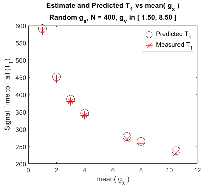
Equation (38) gives a prediction for the first response time. In figure 2(a) we compare the computed value of to the simulation estimate, as we vary the mean of . For each test we select values independently from a uniform distribution with a mean shown in the x-axis. In figure 2(b) we run simulations where form a ramp as . The ramp starts with small and increases so that has a maximum value according to the formula,
The estimates for the random distribution are very close to the predicted value. The ramp “distribution” is not random and it has a large discontinuity at . Although these are clear differences from the uniform distribution, we do not yet understand why the ramp distribution makes the prediction less accurate.


The value in equation (35) determines the first response as it appears in an imaginary expential. The value in equation (36) appears in a real exponential and is negative which indicates a stable solution. This is a dispersion term and tends to disperse the pure frequencies so that the amplitude edges are muted. Figure 3(a) shows a plot with small and figure 3(b) is the same system except the mean value of is larger. This will increase the value of and the resulting peaks are rounder.


The numerics indicate that the system is stable only when are non-negative for all . Setting negative, for a single agent has an immediate effect on system stability. Figure 4(a) shows a simulation where a single agent has negative weight. The plot shows a subset of the flock. The agent with negative weight is shown in green. When the signal to move reaches this agent, the agent moves in the opposite direction and the system starts on an unstable trajectory. If the weight of this single agent was zero then the agents to the left of it would never react to the motion of the leading agent since we are only including nearest neighbor interactions.
Theorem 2.7 states a necessary condition for stability. The difficulty with the theorem is that both and are very small and go to zero as . If we have then the condition is satisfied but changing a single value of to should result in an unstable system. This is difficult to show numerically. In Figure 4, we plot the middle agent for a series of simulations. Each simulation has except for agents centered around agent . For the given simulations, the system is unstable when . The greater the faster the onset of the instability.


A previous work [8] derives a condition on the ratio of successive flock amplitudes. There it is shown that as then the ratio goes to . In Figure 5(a) we plot amplitudes for various distributions of . We do not use the ratio since the first amplitude is close to the initial condition and behaves differently than subsequent peaks. The curves depend on the mean of as altering alters (see equation (36)). We cannot conclusively conclude that this is exactly correct, and more simulation work is required.
We conclude with the realistic system discussed in the introduction. With this example we demonstrate that the tools presented in this paper can be used to analyze more complicated and realistic problems. We make some rough estimates in this next section. A automotive engineer could refine these numbers with more realistic estimates. We model a convoy of trucks traveling on the highway. The convey attempts to keep a fixed spacing between trucks and the trucks are all different. As the convoy travels, lighter cars might, inadvertently, enter the convoy creating a 1-dimensional convoy with very different agents. To use our model, we must estimate the agent weights and . The weights for agent are force coupling divided by the mass of the agent. The mass of a 18 wheel truck is somewhere between 14 and 40 thousand kilograms and the coupling force is determined by the torque of the engine. To make things simpler we shall assume the force divided by the mass produces a given acceleration and we can estimate this acceleration. For example, a truck can accelerate from to mph = m/sec in 1 to 5 minutes. So we take our truck weights in the range,
We insert cars into the convoy by randomly replacing of the agents with lighter cars. Cars, typically, have higher power to mass and so have larger weights. We take a collection of cars that accelerate from to in a range of to seconds, so that for car agents,
To guarantee stability we take where . Increasing , as we’ve seen, will increase the damping. U.S. 18-wheel trucks are typically around meters long. The convoy attempts to keep a distance of meters between the agents.
The simulation results are shown in figure 5(b). The convey of starts with a spacing of meters so is almost long. The first track suddenly increases its speed meters/second and it takes seconds for the signal to reach the last truck. The time duration is long because the weights are small (e.g the trucks accelerate slowly). The distance from the leader to the tail lengthens to m/truck before the tail starts to catch up. The damping is not critical, and the tail overshoots the optimal distance and the entire convey shrinks to m/truck before expanding again. This simulation assumed . There is some evidence that system is more responsive if this condition is removed. We will explore that in a subsequent paper.
References
- [1] N.W. Ashcroft and N.D. Mermin. Solid State Physics. Saunders College, Philadelphia, 1976.
- [2] Pablo E. Baldivieso and J.J.P. Veerman. Stability conditions for coupled autonomous vehicles formations. IEEE Transactions on Control of Network Systems, in press.
- [3] C.E. Cantos, D.K Hammond, and J.J.P. Veerman. Transients in the synchronization of assymmetrically coupled oscillator arrays. The European Physical Journal Special Topics, 225:1115–1125, 2016.
- [4] C.E. Cantos, J.J.P. Veerman, and D.K. Hammond. Signal velocity in oscillator arrays. The European Physical Journal Special Topics, 225:1199–1210, 2016.
- [5] Robert E. Chandler, Robert Herman, and Elliott W. Montroll. Traffic dynamics: Studies in car following. Operations Research, 6:165–184, 1957.
- [6] Freeman J. Dyson. The dynamics of a disordered linear chain. Phys. Rev., 92:1331–1338, Dec 1953.
- [7] He Hao and Prabir Barooah. Stability and robustness of large platoons of vehicle with double-integrator models and nearest neighbor interaction. International Journal of Robust and Nonlinear Control, 23, 12 2013.
- [8] J. Herbrych, A. Chazirakis, N. Christakis, and J.J.P. Veerman. Dynamics of locally coupled agents with next nearest neighbor interaction. Differential Equations and Dynamical Systems, 2017.
- [9] B.S. Kerner. The Physics of Traffic. Springer-Verlag, 2004.
- [10] S. E. Li, Y. Zheng, K. Li, Y. Wu, J. K. Hedrick, F. Gao, and H. Zhang. Dynamical modeling and distributed control of connected and automated vehicles: Challenges and opportunities. IEEE Intelligent Transportation Systems Magazine, 9(3):46–58, 2017.
- [11] Fu Lin, Makan Fardad, and Mihailo R. Jovanovic. Optimal control of vehicular formations with nearest neighbor interactions. IEEE Transactions on Automatic Control, 57(9):2203–2218, 2012.
- [12] Uwe Mackenroth. Robust Control Systems. Springer-Verlag, 2004.
- [13] Wei Ren and Randal Beard. Distributed Consensus in Multi-vehicle Cooperative Control. Springer-Verlag, 2008.
- [14] S. Studli, M. M. Seron, and R. H. Middleton. Vehicular platoons in cyclic interconnections. Automatica, 94:283–293, 2018.