跳到论文正文
W Papers独立论文阅读器 arXiv:2102.08895 论文正文 计算阅读时间 · 0%
引用这篇论文根据当前论文元数据生成,正式投稿前建议核对。


License: arXiv.org perpetual non-exclusive license
arXiv:2102.08895v1 [stat.ML] 17 Feb 2021

On the Fundamental Limits of Exact Inference in Structured Prediction

Hanbyul Lee Affiliation: Department of Statistics Affiliation: Purdue University Affiliation: West Lafayette, IN 47906, USA Email: lee3078@purdue.edu    Kevin Bello Affiliation: Department of Computer Science Affiliation: Purdue University Affiliation: West Lafayette, IN 47906, USA Email: kbellome@purdue.edu    Jean Honorio Affiliation: Department of Computer Science Affiliation: Purdue University Affiliation: West Lafayette, IN 47906, USA Email: jhonorio@purdue.edu
Abstract

Inference is a main task in structured prediction and it is naturally modeled with a graph. In the context of Markov random fields, noisy observations corresponding to nodes and edges are usually involved, and the goal of exact inference is to recover the unknown true label for each node precisely. The focus of this paper is on the fundamental limits of exact recovery irrespective of computational efficiency, assuming the generative process proposed by Globerson et al. 2015. We derive the necessary condition for any algorithm and the sufficient condition for maximum likelihood estimation to achieve exact recovery with high probability, and reveal that the sufficient and necessary conditions are tight up to a logarithmic factor for a wide range of graphs. Finally, we show that there exists a gap between the fundamental limits and the performance of the computationally tractable method of Bello and Honorio 2019, which implies the need for further development of algorithms for exact inference.

1 Introduction

Structured prediction, which is a supervised machine learning that involves structured objects such as sequences and trees, has been utilized in a wide range of domains including sociology, computer vision, natural language processing, and bioinformatics. Examples of the structured prediction problem are community detection, part-of-speech tagging, protein folding, and image segmentation. In various scenarios, one wishes to learn a model representing the interrelation of predicted variables implied by the structure, or is interested on inference after a model has been already learned. Classical methods for learning include conditional random fields (Lafferty et al. 2001) and structured support vector machines (Taskar et al. 2004; Tsochantaridis et al. 2005). In the present paper, we focus on the inference problem.

A great deal of work has addressed the statistical inference over graphs in recent years (Chandrasekaran et al. 2008; Fortunato 2010; Abbe et al. 2014). Typical inference problems in the context of Markov random fields (MRFs) aim to infer the unknown true label corresponding to each node of a given graph, where noisy observations are provided for the labels assigned to edges, or to both edges and nodes. One concrete example is to recover individual opinions in a social network, where one receives noisy measurements of whether two connected individuals have the same opinion or not, and obtains noisy estimates of individual opinions (Foster et al. 2018). Assuming a simple generative model suggested in Globerson et al. 2015, we consider two regimes, one in which only noisy edge observations are given, and one regime in which noisy edge and node observations are collectively provided.

To solve the above inference problems, computationally efficient algorithms have been studied over the past few years. Globerson et al. 2015 presented tight upper and lower bounds of minimum-achievable Hamming error which can be attained by a polynomial-time algorithm for 2D grid graphs. Foster et al. 2018 also developed a polynomial-time solvable algorithm which is based on tree decompositions and can be applied to more general graphs. While the aforementioned works focused on approximate inference, Bello and Honorio 2019 studied the sufficient conditions for exact inference in polynomial time and provided high probability results for general families of graphs. However, the current research works are mainly motivated by computational considerations, and little analysis has been devoted to the statistical complexity of the inference problem irrespective of computational efficiency.

Analyzing the information-theoretic limits associated with the performance of any algorithm is crucial to understand the statistical complexity of the inference problem, as discussed in different contexts (Chen and Xu 2014; Banks et al. 2016; Abbe 2017). In particular, establishing the information-theoretic lower and upper bounds is instrumental in the development of algorithms. If an existent method is computationally tractable and achieves the fundamental limits, then there is little point in suggesting a new algorithm, and if there currently exists a gap between the performance of computationally tractable methods and the fundamental limits, then this situation encourages further elaboration of algorithms.

With this motivation, we develop the fundamental limits of the aforementioned exact inference problems, and compare the limit bounds to those of the currently existent polynomial-time algorithm for exact inference (Bello and Honorio 2019). The information-theoretic limits of a similar problem were studied in Chen et al. 2016, where only a pairwise difference measurement corresponding to each edge was assumed to be given. In contrast to Chen et al. 2016, we consider the node estimate as well as the edge measurement.

The main contribution of this paper consists of providing the necessary condition for any algorithm and the sufficient condition for the optimal strategy (the MLE algorithm) to exactly recover the true unknown labels with probability 1−o⁡(n)1-o(n), where nn is the number of nodes of a given graph. We find that the conditions involve multiple graphical factors such as the number of edges, the maximum degree of the graph, and the Cheeger constant. Our results apply to general graphs, and especially to complete graphs, regular expanders and star graphs, we show that the sufficient and necessary conditions are tight up to a logarithmic factor. Furthermore, we reveal that the error bound of the MLE algorithm decays much faster than that of the polynomial-time algorithm in Bello and Honorio 2019, eliciting a gap between the optimal method and the currently existent tractable algorithm.

The remainder of this paper is organized as follows. In Section 2, we describe the formal problem setup and introduce terminology and notation. We develop sufficient and necessary conditions for exact recovery where only edge observations are given in Section 3, and where edge and node observations are both given in Section 4. In both sections, we provide an illustration of the fundamental limit bounds for a few examples of graphs. Section 5 concludes the paper with a summary of our findings and a discussion of future works. The proofs of the theorems are deferred to the appendices.

2 Preliminaries

We first introduce the inference problem, graph terminology and notation used throughout the paper.

2.1 Exact Inference Problem

We assume that there is a known undirected connected graph 𝒢=(𝒱,ℰ)\mathcal{G}=(\mathcal{V},\mathcal{E}) with nn nodes, where 𝒱={1,…,n}\mathcal{V}=\{1,\dots,n\}. Each node has an unknown true label yi∗∈{−1,1}y_{i}^{*}\in\{-1,1\}, i∈𝒱i\in\mathcal{V}, and we denote the true label vector by 𝒚∗=(y1∗,⋯,yn∗)⊤\boldsymbol{y}^{*}=(y_{1}^{*},\cdots,y_{n}^{*})^{\top}. We suppose that nature picks 𝒚∗\boldsymbol{y}^{*} from a uniform distribution with support 𝒴={−1,1}n\mathcal{Y}=\{-1,1\}^{n}, |𝒴|=2n|\mathcal{Y}|=2^{n}. A set of noisy observations X∈𝒳X\in\mathcal{X} and 𝒄∈𝒞={−1,1}n\boldsymbol{c}\in\mathcal{C}=\{-1,1\}^{n}, where XX and 𝒄\boldsymbol{c} correspond to edges and nodes respectively, is assumed to be generated from 𝒚∗\boldsymbol{y}^{*} by the following process:

ℙ⁡(Xi​j=yi∗​yj∗|𝒚∗)=1−ℙ⁡(Xi​j=−yi∗​yj∗|𝒚∗)=1−p\displaystyle\mathbb{P}\big(X_{ij}=y_{i}^{*}y_{j}^{*}\big|\boldsymbol{y}^{*}\big)=1-\mathbb{P}\big(X_{ij}=-y_{i}^{*}y_{j}^{*}\big|\boldsymbol{y}^{*}\big)=1-p
ℙ⁡(ck=yk∗|𝒚∗)=1−ℙ⁡(ck=−yk∗|𝒚∗)=1−q\displaystyle\mathbb{P}\big(c_{k}=y_{k}^{*}\big|\boldsymbol{y}^{*}\big)=1-\mathbb{P}\big(c_{k}=-y_{k}^{*}\big|\boldsymbol{y}^{*}\big)=1-q

for (i,j)∈ℰ(i,j)\in\mathcal{E} and k∈𝒱k\in\mathcal{V}. The parameters pp and qq are fixed and between 00 and 12\frac{1}{2}. Note that we set XX as an n×nn\times n upper triangular matrix with Xi​j=0X_{ij}=0 for (i,j)∉ℰ(i,j)\notin\mathcal{E}, so that the cardinality of 𝒳\mathcal{X} is |𝒳|=2|ℰ||\mathcal{X}|=2^{|\mathcal{E}|}. We consider two regimes where (1) only noisy edge observation XX is given and (2) noisy edge and node observations XX and 𝒄\boldsymbol{c} are both given. The goal is to exactly recover the true label vector 𝒚∗\boldsymbol{y}^{*} (i.e., with zero Hamming error) in each regime.

2.2 Graph Terminology

We denote the degree of iith node by Δi\Delta_{i}, and the maximum degree of nodes by Δmax:=maxi∈𝒱​Δi\Delta_{\max}:=\underset{i\in\mathcal{V}}{\max}~\Delta_{i}. For any subset S⊆𝒱S\subseteq\mathcal{V}, ScS^{c} indicates its complement and we let ℰ⁡(S,Sc)\mathcal{E}(S,S^{c}) denote the collection of all edges going from a node in SS to a node outside of SS, i.e., ℰ(S,Sc):={(i,j)∈ℰ:i∈S,j∈Scori∈Sc,j∈S}\mathcal{E}(S,S^{c}):=\{(i,j)\in\mathcal{E}:i\in S,j\in S^{c}~\text{or}~i\in S^{c},j\in S\}. |ℰ⁡(S,Sc)||\mathcal{E}(S,S^{c})| represents the number of edges between SS and ScS^{c}. The Cheeger constant of a graph 𝒢\mathcal{G} is defined as ϕ𝒢:=minS⊆𝒱,1≤|S|≤⌊n2⌋​|ℰ⁡(S,Sc)||S|\phi_{\mathcal{G}}:=\underset{S\subseteq\mathcal{V},1\leq|S|\leq{{}_{\lfloor}}\frac{n}{2}{{}_{\rfloor}}}{\min}\frac{|\mathcal{E}(S,S^{c})|}{|S|}, which is also called edge expansion.

In what follows, we introduce several classes of graphs which are taken as examples in this paper.

  1. 1.

    Complete graph: A graph is said to be complete if every pair of distinct nodes is connected by an edge.

  2. 2.

    Chain graph: A chain graph is a sequence of nodes connected by edges. The length of a chain is the number of edges, which is the number of nodes minus one.

  3. 3.

    Star graph: A star graph has one internal node which is connected to all the others. The other nodes are not connected to each other.

  4. 4.

    Regular expander: A dd-regular expander with constant C>0C>0 is a graph whose nodes have the same degree dd, and which satisfies that for every subset S⊆𝒱S\subseteq\mathcal{V} with |S|≤n2|S|\leq\frac{n}{2}, |ℰ⁡(S,Sc)|≥C​d​|S||\mathcal{E}(S,S^{c})|\geq Cd|S|.

A chain graph and a star graph are examples of tree graphs, in which any two nodes are connected by exactly one path of edges. Note that a graph is a tree graph if and only if a graph has exactly n−1n-1 edges. Key graphical metrics of the above example graphs are summarized in Table 1.

Table 1: Graphical Metrics of Example Graphs.
Type of Graph |ℰ||\mathcal{E}| Δmax\Delta_{\max} ϕ𝒢\phi_{\mathcal{G}}
Complete graph (n2)\binom{n}{2} n−1n-1 n/2n/2
Chain graph n−1n-1 22 2/n2/n
Star graph n−1n-1 n−1n-1 11
dd-regular expander n​d/2nd/2 dd ≥C​d\geq Cd

2.3 Other Notation

The number ee and log⁡(⋅)\log(\cdot) indicate Euler’s number and the natural logarithm. The function H∗​(p):=−p​log⁡p−(1−p)​log⁡(1−p)H^{*}(p):=-p\log p-(1-p)\log(1-p) stands for the binary entropy function. 𝔼W​[⋅]\mathbb{E}_{W}[\cdot] represents the expectation with respect to a random variable WW. The indicator function is denoted by 𝕀⁡[⋅]\mathbb{I}[\cdot]. We denote by a∧ba\wedge b and a∨ba\vee b the minimum and maximum between aa and bb, respectively, where aa and bb are two scalars. We use CC, C′C^{\prime}, C′′,…C^{\prime\prime},\dots to denote universal constants independent of (n,p,q,|ℰ|,ϕ𝒢n,p,q,|\mathcal{E}|,\phi_{\mathcal{G}}). The notation f⁡(n)=o⁡(g⁡(n))f(n)=o(g(n)) means limn→∞f⁡(n)/g⁡(n)=0\lim_{n\rightarrow\infty}f(n)/g(n)=0; f⁡(n)=Ω⁡(g⁡(n))f(n)=\Omega(g(n)) means that there exists a constant CC such that f⁡(n)≥C​g​(n)f(n)\geq Cg(n) asymptotically; f⁡(n)=O⁡(g⁡(n))f(n)=O(g(n)) means that there exists a constant CC such that f⁡(n)≤C​g​(n)f(n)\leq Cg(n) asymptotically; f⁡(n)=Θ⁡(g⁡(n))f(n)=\Theta(g(n)) means that there exists constants CC and C′C^{\prime} such that C​g​(n)≤f⁡(n)≤C′​g​(n)Cg(n)\leq f(n)\leq C^{\prime}g(n) asymptotically.

3 Regime I: Edge Observations Only

Now we derive the information-theoretic limits of exact recovery where only noisy edge observations are given. We first introduce the lower bound of the minimax error probability and the lower bound of the probability of success of the maximum likelihood estimator which is a minimax optimal estimator. From the two results, we derive the necessary and the sufficient conditions of exact recovery regardless of its computational complexity. Then we illustrate the limit bounds for several examples of graphs.

3.1 Minimax Lower Bound

We first develop the lower bound of the probability for any algorithm to fail to exactly recover the true label vector 𝒚∗\boldsymbol{y}^{*}.

Theorem 1.

Let 𝒢=(𝒱,ℰ)\mathcal{G}=(\mathcal{V},\mathcal{E}) be an undirected connected graph with nn nodes, Cheeger constant ϕ𝒢\phi_{\mathcal{G}}, and maximum node degree Δmax\Delta_{\max}. Consider a family of distributions 𝒫\mathcal{P} over 𝒴×𝒳\mathcal{Y}\times\mathcal{X}. Then, for the inference problem in Section 2.1 in which only the noisy edge observation X∈𝒳X\in\mathcal{X} is given, the minimax probability of error is bounded below as follows:

inf𝒚^:𝒳→𝒴supP∈𝒫ℙ(𝒚∗,X)∼P[𝒚^(X)≠𝒚∗]≥max{f1,g1,g1∗}\inf_{\hat{\boldsymbol{y}}:\mathcal{X}\to\mathcal{Y}}\sup_{P\in\mathcal{P}}\mathbb{P}_{(\boldsymbol{y}^{*},X)\sim P}\big[\hat{\boldsymbol{y}}(X)\neq\boldsymbol{y}^{*}\big]\geq\max\big\{f_{1},g_{1},g^{*}_{1}\big\}

where

f1\displaystyle f_{1} :=12∑m=0Δmax(Δmaxm)[{(1−p)mpΔmax−m}\displaystyle:=\frac{1}{2}\sum_{m=0}^{\Delta_{\max}}\binom{\Delta_{\max}}{m}\bigg[\Big\{(1-p)^{m}p^{\Delta_{\max}-m}\Big\}
∧{pm(1−p)Δmax−m}],\displaystyle~~~~~~~~~~~~~~~~~~~~~~~~~~~\wedge\Big\{p^{m}(1-p)^{\Delta_{\max}-m}\Big\}\bigg],
g1\displaystyle g_{1} :=n−1n−|ℰ|n⋅(1−H∗​(p)log⁡2),\displaystyle:=\frac{n-1}{n}-\frac{|\mathcal{E}|}{n}\cdot\bigg(1-\frac{H^{*}(p)}{\log 2}\bigg),
g1∗\displaystyle g^{*}_{1} :=g1+(|ℰ|​log⁡2−κ1)∨0n​log⁡2⋅𝕀[(1−p)|ℰ|≤e−1].\displaystyle:=g_{1}+\frac{\big(|\mathcal{E}|\log 2-\kappa_{1}\big)\vee 0}{n\log 2}\cdot\mathbb{I}\big[(1-p)^{|\mathcal{E}|}\leq e^{-1}\big].

Here, κ1:=−|ℰ|​log⁡(1−p)​{2​(1−p)}|ℰ|​𝔼B​[τ⁡(B)2n]+{2​(1−p)}|ℰ|​𝔼B​[−τ⁡(B)2n​log⁡(τ⁡(B)2n)]\kappa_{1}:=-|\mathcal{E}|\log(1-p)\{2(1-p)\}^{|\mathcal{E}|}\mathbb{E}_{B}\big[\frac{\tau(B)}{2^{n}}\big]+\{2(1-p)\}^{|\mathcal{E}|}\mathbb{E}_{B}\big[-\frac{\tau(B)}{2^{n}}\log\big(\frac{\tau(B)}{2^{n}}\big)\big]. In addition, τ⁡(B):=2​(p1−p)B+∑k=1n−1(nk)​(p1−p)(ϕ𝒢⋅{k∧(n−k)}−B)∨0\tau(B):=2\big(\frac{p}{1-p}\big)^{B}+\sum_{k=1}^{n-1}\binom{n}{k}\big(\frac{p}{1-p}\big)^{(\phi_{\mathcal{G}}\cdot\{k\wedge(n-k)\}-B)\vee 0} and B∼Bin​(|ℰ|−n+1,12)B\sim\text{Bin}(|\mathcal{E}|-n+1,~\frac{1}{2}).

The bound of f1f_{1} is derived from Assouad’s lemma, and g1g_{1} and g1∗g_{1}^{*} are obtained from Fano’s inequality. When applying Fano’s inequality, we use two different strategies to bound the mutual information and then derive g1g_{1} and g1∗g_{1}^{*} from them respectively. See Appendix A.2 for the details.

Figure 1: Graphical illustration of the functions f1f_{1} and g1g_{1} with respect to the parameter p∈[0,12]p\in[0,\frac{1}{2}] in Theorem 1. The green triangle indicates the area where the function f1f_{1} has its function value. The red and blue lines represent the function g1g_{1} when |ℰ|=n−1|\mathcal{E}|=n-1 and |ℰ|>n−1|\mathcal{E}|>n-1, respectively. The function g1g_{1} always has a positive value when |ℰ|=n−1|\mathcal{E}|=n-1, and when |ℰ|>n−1|\mathcal{E}|>n-1, g1g_{1} has its yy-intercept at n−1n−|ℰ|n\frac{n-1}{n}-\frac{|\mathcal{E}|}{n} and its xx-intercept between 0.34−n−12​|ℰ|0.34-\frac{n-1}{2|\mathcal{E}|} and 0.5−n−12​|ℰ|0.5-\frac{n-1}{2|\mathcal{E}|}.

From Figure 1, we can verify which of the functions f1f_{1} or g1g_{1} achieves the maximum in different situations. For instance, when |ℰ|=n−1|\mathcal{E}|=n-1, i.e., the graph 𝒢\mathcal{G} has a tree structure, the function g1g_{1} is always greater than f1f_{1}. If |ℰ||\mathcal{E}| gets larger than n−1n-1, then the function g1g_{1} has a negative value when pp is small, therefore f1f_{1} achieves the maximum for small pp. As n−1|ℰ|\frac{n-1}{|\mathcal{E}|} decreases, the range of pp where f1>g1f_{1}>g_{1} holds gets larger.

The function g1∗g_{1}^{*} is always greater than or equal to g1g_{1} since the added value to g1g_{1} in g1∗g_{1}^{*} is non-negative. In most cases, g1g_{1} and g1∗g_{1}^{*} are the same. Exceptionally, when |ℰ|>n−1|\mathcal{E}|>n-1 (i.e., 𝒢\mathcal{G} is not a tree graph), nn is small and pp is large, g1∗g_{1}^{*} becomes greater than g1g_{1}, which can be also verified from the illustration in Section 3.3.

We add a remark about the possibility to improve the limit bound in Theorem 1.

Remark 1.

We can observe that κ1\kappa_{1} decreases as ϕ𝒢\phi_{\mathcal{G}} increases when (1−p)|ℰ|≤e−1(1-p)^{|\mathcal{E}|}\leq e^{-1} holds. Hence, g1∗g_{1}^{*} increases as ϕ𝒢\phi_{\mathcal{G}} increases, which does not match with the intuition that exact recovery is easier for a graph 𝒢\mathcal{G} with larger Cheeger constant. This implies that there is room for improvement on the bound in Theorem 1.

Now, we derive a corollary from Theorem 1, which induces a necessary condition for any algorithm to exactly recover the true label 𝒚∗\boldsymbol{y}^{*}.

Corollary 1 (Necessary Condition).

Under the same assumptions as in Theorem 1, if the following condition holds:

|ℰ|⋅(1−H∗​(p)log⁡2)≤n2−1,|\mathcal{E}|\cdot\bigg(1-\frac{H^{*}(p)}{\log 2}\bigg)\leq\frac{n}{2}-1, (1)

then inf𝐲^:𝒳→𝒴supP∈𝒫ℙ(𝐲∗,X)∼P[𝐲^(X)≠𝐲∗]≥12\underset{\hat{\boldsymbol{y}}:\mathcal{X}\to\mathcal{Y}}{\inf}\underset{P\in\mathcal{P}}{\sup}\mathbb{P}_{(\boldsymbol{y}^{*},X)\sim P}\big[\hat{\boldsymbol{y}}(X)\neq\boldsymbol{y}^{*}\big]\geq\frac{1}{2}, that is, any algorithm fails to exactly recover the true node labels with probability greater than half.

Proof.

Since g1∗g_{1}^{*} is always greater than or equal to g1g_{1} and f1f_{1} is smaller than half, it is sufficient to derive the condition in which g1g_{1} becomes larger than half. ∎

Figure 2: Graphical illustration of the functions 1−H∗​(p)log⁡21-\frac{H^{*}(p)}{\log 2} (red line) and (1−2​p)2(1−p)​(1+4​p)\frac{(1-2p)^{2}}{(1-p)(1+4p)} (blue line) in Corollary 1 and 2, respectively. Two functions are close to each other on the domain p∈[0,12]p\in[0,\frac{1}{2}]. When p≤0.0443p\leq 0.0443, (1−2​p)2(1−p)​(1+4​p)\frac{(1-2p)^{2}}{(1-p)(1+4p)} is slightly greater than 1−H∗​(p)log⁡21-\frac{H^{*}(p)}{\log 2}, and the reverse holds when p>0.0443p>0.0443.

Note that the opposite of the condition (1) provides the necessary condition for exact recovery. The red line in Figure 2 graphically illustrates the function 1−H∗​(p)log⁡21-\frac{H^{*}(p)}{\log 2}, which decreases from 11 to 00 as pp increases from 00 to 1/21/2. This implies that it becomes harder to satisfy the necessary condition as pp gets close to 1/21/2. On the other hand, we can observe that the necessary condition holds for any graph if 1−H∗​(p)log⁡2>121-\frac{H^{*}(p)}{\log 2}>\frac{1}{2} (i.e., pp is smaller than 0.110.11), because |ℰ|⋅(1−H∗​(p)log⁡2)>n−12>n2−1|\mathcal{E}|\cdot\big(1-\frac{H^{*}(p)}{\log 2}\big)>\frac{n-1}{2}>\frac{n}{2}-1.

3.2 Maximum Likelihood Estimator

Given the noisy edge observations only, the Maximum Likelihood Estimator (MLE) of the model presented in Section 2.1 is derived as follows:

𝒚^m​l​e​(X):=arg⁡max𝒚∈𝒴​𝒚T​X​𝒚.\hat{\boldsymbol{y}}_{mle}(X):=\underset{\boldsymbol{y}\in\mathcal{Y}}{\arg\max}~~~\boldsymbol{y}^{T}X\boldsymbol{y}. (2)

The optimization problem (2) is known to be NP-hard, so it cannot be used in practice. However, the MLE method is a minimax-optimal strategy in our problem 11 1 The Bayes estimator for the zero-one loss is the Maximum A-Posteriori (MAP) estimator. Since we assume that 𝒚∗\boldsymbol{y}^{*} is uniformly distributed, the Bayes estimator is minimax optimal and the MLE is equivalent to the MAP estimator. Hence, the MLE is minimax optimal. See Bickel and Doksum 2015 for details., so it serves as a benchmark for tractable algorithms.

We first derive the lower bound of the probability for the MLE algorithm to exactly recover the true label 𝒚∗\boldsymbol{y}^{*} up to a global flip of the labels.

Theorem 2.

Let 𝒢=(𝒱,ℰ)\mathcal{G}=(\mathcal{V},\mathcal{E}) be an undirected connected graph with nn nodes and Cheeger constant ϕ𝒢\phi_{\mathcal{G}}. Let h1​(p,z):=exp⁡[−(1−2​p)2​z43​(1−p)​(1+4​p)]h_{1}(p,z):=\exp\Big[-\frac{(1-2p)^{2}z}{\frac{4}{3}(1-p)(1+4p)}\Big]. Then, for the inference problem in Section 2.1 in which only the noisy edge observation XX is given, the MLE algorithm in (2) returns a solution 𝐲^m​l​e​(X)∈{𝐲∗,−𝐲∗}\hat{\boldsymbol{y}}_{mle}(X)\in\{\boldsymbol{y}^{*},-\boldsymbol{y}^{*}\} with probability at least

1−∑k=1⌊n2⌋(nk)​h1​(p,ϕ𝒢​k).1-\sum_{k=1}^{\lfloor\frac{n}{2}\rfloor}\binom{n}{k}h_{1}(p,\phi_{\mathcal{G}}k).

The Bernstein inequality and the union bound are mainly used in the proof (See Appendix A.3.) Note that h1​(p,ϕ𝒢​k)h_{1}(p,\phi_{\mathcal{G}}k) decreases as pp decreases or ϕ𝒢\phi_{\mathcal{G}} increases, that is, the lower bound of the probability of success becomes large for small pp and large ϕ𝒢\phi_{\mathcal{G}} (e.g., large dd in regular expanders.) We will illustrate the bounds for several examples in Section 3.3.

Comparison to Tractable Algorithm. We compare the above lower bound for the MLE algorithm to that of a polynomial-time solvable algorithm introduced in Bello and Honorio 2019. The upper bound of the error probability of the tractable algorithm is as follows:

ϵ1:=2​n⋅e−3​(1−2​p)2​ϕ𝒢41536​Δmax3​p​(1−p)+32​(1−2​p)​(1−p)​ϕ𝒢2​Δmax.\epsilon_{1}:=2n\cdot e^{\frac{-3(1-2p)^{2}\phi_{\mathcal{G}}^{4}}{1536\Delta_{\max}^{3}p(1-p)+32(1-2p)(1-p)\phi_{\mathcal{G}}^{2}\Delta_{\max}}}. (3)

If ϕ𝒢=Ω⁡(n)\phi_{\mathcal{G}}=\Omega(n) (e.g., complete graph, regular expander with d=Ω⁡(n)d=\Omega(n)), we can derive ∑k=1⌊n2⌋(nk)h1(p,ϕ𝒢k)ϵ1=O⁡(exp⁡(−C​(1−2​p)2​n(1−p)​(1+4​p)))\frac{\sum_{k=1}^{{}_{\lfloor}\frac{n}{2}_{\rfloor}}\binom{n}{k}h_{1}(p,\phi_{\mathcal{G}}k)}{\epsilon_{1}}=O\big(\exp\big(-\frac{C(1-2p)^{2}n}{(1-p)(1+4p)}\big)\big) for some positive constant CC (see Appendix A.4.) Hence, ∑k=1⌊n2⌋(nk)h1(p,ϕ𝒢k)\sum_{k=1}^{{}_{\lfloor}\frac{n}{2}_{\rfloor}}\binom{n}{k}h_{1}(p,\phi_{\mathcal{G}}k) decays much faster than ϵ1\epsilon_{1}, and this implies that the currently existent and tractable method does not achieve the fundamental limits.

Next, we derive from Theorem 2 the sufficient condition for the MLE algorithm to exactly recover the true label with high probability.

Corollary 2 (Sufficient Condition).

Under the same assumptions as in Theorem 2, if the following condition holds:

ϕ𝒢⋅(1−2​p)2(1−p)​(1+4​p)≥83​log⁡n,\phi_{\mathcal{G}}\cdot\frac{(1-2p)^{2}}{(1-p)(1+4p)}\geq\frac{8}{3}\log n, (4)

then the optimal solution to the MLE algorithm in (2) fulfills 𝐲^m​l​e​(X)∈{𝐲∗,−𝐲∗}\hat{\boldsymbol{y}}_{mle}(X)\in\{\boldsymbol{y}^{*},-\boldsymbol{y}^{*}\} with probability =1−2​n−1=1-2n^{-1}.

Tightness of Sufficient and Necessary Conditions. One important question is how tight the necessary and the sufficient conditions derived in Corollary 1 and 2 are. In Figure 2, we observe that the functions 1−H∗​(p)log⁡21-\frac{H^{*}(p)}{\log 2} and (1−2​p)2(1−p)​(1+4​p)\frac{(1-2p)^{2}}{(1-p)(1+4p)} (red and blue lines, respectively) are almost the same. Hence, the condition (4) can be written as ϕ𝒢⋅(1−H∗​(p)log⁡2)≥C​log⁡n\phi_{\mathcal{G}}\cdot\big(1-\frac{H^{*}(p)}{\log 2}\big)\geq C\log n for some constant CC. Then, if |ℰ|/ϕ𝒢=Θ⁡(n)|\mathcal{E}|/\phi_{\mathcal{G}}=\Theta(n) holds (e.g., complete graph, star graph, regular expander), the condition (4) reduces to |ℰ|⋅(1−H∗​(p)log⁡2)≥C′​n​log⁡n|\mathcal{E}|\cdot\big(1-\frac{H^{*}(p)}{\log 2}\big)\geq C^{\prime}n\log n, and the sufficient and necessary conditions are thus tight up to at most a logarithmic factor.

3.3 Illustration

Figure 3: Minimax lower bound in Theorem 1 (first row), lower bound of probability of success of the MLE algorithm in Theorem 2 (second row), and lower bound of probability of success of the tractable algorithm in Bello and Honorio 2019 (third row). The first and second columns correspond to regular expanders and tree graphs, respectively. The x-axis indicates the parameter p∈[0,12]p\in[0,\frac{1}{2}]. Different colors and line-types represent different numbers of nodes (nn) and the degrees of regular expanders (dd).

Figure 3 illustrates the bounds of the probabilities in Theorem 1 and 2, and the lower bound of the probability of success of the polynomial-time algorithm (which is 1−ϵ11-\epsilon_{1}) for regular expanders and tree graphs. Results for more types of graphs are provided in Appendix A.6.

The first thing we can observe is the gap between the fundamental limits and the performance of the polynomial-time algorithm. In regular expanders, we observe that the success of the MLE algorithm is guaranteed with higher probability as the degree dd increases, while the lower bound of the probability of success of the polynomial-time algorithm is zero even with d=60d=60. In fact, dd must be about 20002000 so that when pp is close to 00, the lower bound gets close to 11 in the case of polynomial-time algorithm (See Appendix A.6.)

Next, we can observe that as nn increases, the minimax lower bound increases and the lower bound of the probability of success of the MLE algorithm decreases for tree graphs and regular expanders. That is, the exact recovery problem becomes difficult as the number of nodes nn gets larger for those graph classes. On the other hand, when nn is fixed, the minimax lower bound decreases and the lower bound of the probability of success of the MLE algorithm increases as dd increases in regular expanders. Since the degree dd in regular expanders has the same effect on the bounds as the number of nodes nn in the complete graph in our results, the exact recovery problem becomes easier as nn increases for complete graphs. Thus, the effect of nn on the fundamental limits is different between complete graphs and the aforementioned graphs.

Lastly, looking in detail at the minimax lower bounds, we can first observe that there exist two non-smooth points when n=4n=4 and d=2d=2 in the regular expander. They are the points in which the function achieving the maximum changes. The maximum lower bound is achieved by f1f_{1}, g1g_{1} and g1∗g_{1}^{*} in sequence as pp increases from 00 to 1/21/2. When nn and dd become greater, g1g_{1} and g1∗g_{1}^{*} become the same, so either f1f_{1} or g1g_{1} achieves the maximum. In the case of tree graphs, the function g1g_{1} always achieves the maximum, so that there is no non-smooth point.

4 Regime II: Edge and Node Observations

Now we consider the extended regime in which noisy edge and node observations are collectively provided. Recall that the noisy node observation is denoted by the vector 𝒄\boldsymbol{c}. The iith element of 𝒄\boldsymbol{c} has the same value as the true label yi∗y_{i}^{*}, i=1,⋯,ni=1,\cdots,n, with probability 1−q1-q, q∈[0,12]q\in[0,\frac{1}{2}]. In addition to (n,p,|ℰ|,Δmax,ϕ𝒢)(n,p,|\mathcal{E}|,\Delta_{\max},\phi_{\mathcal{G}}), the parameter qq will be involved in the results of this section.

4.1 Minimax Lower Bound

We first derive the minimax lower bound of the probability of failure as follows.

Theorem 3.

Let 𝒢=(𝒱,ℰ)\mathcal{G}=(\mathcal{V},\mathcal{E}) be an undirected connected graph with nn nodes, Cheeger constant ϕ𝒢\phi_{\mathcal{G}}, and maximum node degree Δmax\Delta_{\max}. Consider a family of distributions 𝒫\mathcal{P} over 𝒴×(𝒳×𝒞)\mathcal{Y}\times(\mathcal{X}\times\mathcal{C}). Then, for the inference problem in Section 2.1 in which the noisy edge and node observations X∈𝒳X\in\mathcal{X} and 𝐜∈𝒞\boldsymbol{c}\in\mathcal{C} are given, the minimax probability of error is bounded below as follows:

inf𝒚^:𝒳×𝒞→𝒴supP∈𝒫ℙ(𝒚∗,(X,𝒄))∼P[𝒚^(X,𝒄)≠𝒚∗]≥max⁡{f2,g2,g2∗}\underset{\hat{\boldsymbol{y}}:\mathcal{X}\times\mathcal{C}\to\mathcal{Y}}{\inf}~\underset{P\in\mathcal{P}}{\sup}~\mathbb{P}_{(\boldsymbol{y}^{*},(X,\boldsymbol{c}))\sim P}\big[\hat{\boldsymbol{y}}(X,\boldsymbol{c})\neq\boldsymbol{y}^{*}\big]\\ \geq\max\big\{f_{2},g_{2},g^{*}_{2}\big\}

where

f2:=12​∑m=0Δmax(Δmaxm)\displaystyle f_{2}:=\frac{1}{2}\sum_{m=0}^{\Delta_{\max}}\binom{\Delta_{\max}}{m}
×({pm​(1−p)Δmax−m​q}∧{(1−p)m​pΔmax−m​(1−q)}CLOSE\displaystyle\times\bigg(\big\{p^{m}(1-p)^{\Delta_{\max}-m}q\big\}\wedge\big\{(1-p)^{m}p^{\Delta_{\max}-m}(1-q)\big\}
OPEN+{pm​(1−p)Δmax−m​(1−q)}∧{(1−p)m​pΔmax−m​q}),\displaystyle+\big\{p^{m}(1-p)^{\Delta_{\max}-m}(1-q)\big\}\wedge\big\{(1-p)^{m}p^{\Delta_{\max}-m}q\big\}\bigg),
g2:=n−1n−|ℰ|n​(1−H∗​(p)log⁡2)−(1−H∗​(q)log⁡2),\displaystyle g_{2}:=\frac{n-1}{n}-\frac{|\mathcal{E}|}{n}\bigg(1-\frac{H^{*}(p)}{\log 2}\bigg)-\bigg(1-\frac{H^{*}(q)}{\log 2}\bigg),
g2∗:=g2+{(|ℰ|+n)​log⁡2−κ2}∨0n​log⁡2\displaystyle g^{*}_{2}:=g_{2}+\frac{\big\{(|\mathcal{E}|+n)\log 2-\kappa_{2}\big\}\vee 0}{n\log 2}
×𝕀[(1−p)|ℰ|(1−q)n≤e−1].\displaystyle\hskip 110.00017pt\times\mathbb{I}\big[(1-p)^{|\mathcal{E}|}(1-q)^{n}\leq e^{-1}\big].

Here, κ2={−|ℰ|​log⁡(1−p)−n​log⁡(1−q)}⋅12​{2​(1−q)}n​{2​(1−p)}|ℰ|​𝔼B​[τ⁡(B)2n]+{−|ℰ|​log⁡(1−p)+n​log⁡2}⋅12​{2​(1−p)}|ℰ|⋅12n+12​{2​(1−q)}n​{2​(1−p)}|ℰ|​𝔼B​[−τ⁡(B)2n​log⁡(τ⁡(B)2n)]\kappa_{2}=\{-|\mathcal{E}|\log(1-p)-n\log(1-q)\}\cdot\frac{1}{2}\{2(1-q)\}^{n}\{2(1-p)\}^{|\mathcal{E}|}\mathbb{E}_{B}\big[\frac{\tau(B)}{2^{n}}\big]+\{-|\mathcal{E}|\log(1-p)+n\log 2\}\cdot\frac{1}{2}\{2(1-p)\}^{|\mathcal{E}|}\cdot\frac{1}{2^{n}}+\frac{1}{2}\{2(1-q)\}^{n}\{2(1-p)\}^{|\mathcal{E}|}\mathbb{E}_{B}\big[-\frac{\tau(B)}{2^{n}}\log\big(\frac{\tau(B)}{2^{n}}\big)\big]. In addition, τ⁡(B):=2​(p1−p)B+∑k=1n−1(nk)​(p1−p)(ϕ𝒢⋅{k∧(n−k)}−B)∨0\tau(B):=2\big(\frac{p}{1-p}\big)^{B}+\sum_{k=1}^{n-1}\binom{n}{k}\big(\frac{p}{1-p}\big)^{(\phi_{\mathcal{G}}\cdot\{k\wedge(n-k)\}-B)\vee 0} and B∼Bin​(|ℰ|−n+1,12)B\sim\text{Bin}(|\mathcal{E}|-n+1,~\frac{1}{2}).

As in Theorem 1, f2f_{2} is derived from Assouad’s lemma and g2g_{2} and g2∗g_{2}^{*} are obtained from Fano’s inequality. See Appendix A.7 for the detailed proof.

Figure 4: Graphical illustration of the functions f2f_{2} and g2g_{2} with respect to the parameter p∈[0,12]p\in[0,\frac{1}{2}] in Theorem 3. The green triangle indicates the area where the function f2f_{2} has its function value. The red and blue lines represent the function g2g_{2} when |ℰ|=n−1,q=0.5|\mathcal{E}|=n-1,q=0.5 and |ℰ|>n−1,q<0.5|\mathcal{E}|>n-1,q<0.5, respectively. When |ℰ|=n−1|\mathcal{E}|=n-1 and q=0.5q=0.5, the function g2g_{2} always has a positive value, and the plot goes downward as |ℰ||\mathcal{E}| increases or qq decreases. When |ℰ|>n−1|\mathcal{E}|>n-1 and q<0.5q<0.5, g2g_{2} has its yy-intercept at n−1n−|ℰ|n−(1−H∗​(q)log⁡2)\frac{n-1}{n}-\frac{|\mathcal{E}|}{n}-\Big(1-\frac{H^{*}(q)}{\log 2}\Big) and its xx-intercept between 0.34−n−12​|ℰ|+n2​|ℰ|​(1−H∗​(q)log⁡2)0.34-\frac{n-1}{2|\mathcal{E}|}+\frac{n}{2|\mathcal{E}|}\Big(1-\frac{H^{*}(q)}{\log 2}\Big) and 0.5−n−12​|ℰ|+n2​|ℰ|​(1−H∗​(q)log⁡2)0.5-\frac{n-1}{2|\mathcal{E}|}+\frac{n}{2|\mathcal{E}|}\Big(1-\frac{H^{*}(q)}{\log 2}\Big).

We can verify from Figure 4 which of the functions f2f_{2} or g2g_{2} achieves the maximum in different situations. The figure is similar to Figure 1, but the difference is that the parameter q∈[0,12]q\in[0,\frac{1}{2}] is involved in this case. First, the function g2g_{2} is greater than the function f2f_{2} for any pp only when |ℰ|=n−1|\mathcal{E}|=n-1 and q=0.5q=0.5. As |ℰ||\mathcal{E}| increases or qq decreases, the yy-intercept of function g2g_{2} becomes negative and smaller, thus f2f_{2} has a greater value than g2g_{2} for small pp. Especially, when qq is close to zero, the maximal function value of g2g_{2} becomes negative, therefore f2f_{2} is greater than g2g_{2} for any pp in this case.

The function g2∗g_{2}^{*} is always greater than or equal to g2g_{2}, and in most cases, they are equivalent. An exceptional case is when pp and qq are both close to 12\frac{1}{2}. If p,q≈12p,q\approx\frac{1}{2}, we can derive that κ2≈(|ℰ|+n)​log⁡2⋅12​(1+12n)\kappa_{2}\approx(|\mathcal{E}|+n)\log 2\cdot\frac{1}{2}\big(1+\frac{1}{2^{n}}\big), that is, (|ℰ|+n)​log⁡2−κ2≈(|ℰ|+n)​log⁡2⋅(12−12n+1)(|\mathcal{E}|+n)\log 2-\kappa_{2}\approx(|\mathcal{E}|+n)\log 2\cdot\big(\frac{1}{2}-\frac{1}{2^{n+1}}\big). Since this is always positive, g2∗g_{2}^{*} becomes strictly greater than g2g_{2}.

Now we derive from Theorem 3 the necessary condition for any algorithm to exactly recover the true label 𝒚∗\boldsymbol{y}^{*}.

Corollary 3 (Necessary Condition).

Under the same assumptions as in Theorem 3, if the following condition holds:

|ℰ|​(1−H∗​(p)log⁡2)+n⁡(1−H∗​(q)log⁡2)≤n2−1,|\mathcal{E}|\bigg(1-\frac{H^{*}(p)}{\log 2}\bigg)+n\bigg(1-\frac{H^{*}(q)}{\log 2}\bigg)\leq\frac{n}{2}-1, (5)

then inf𝐲^:𝒳×𝒞→𝒴supP∈𝒫ℙ(𝐲∗,(X,𝐜))∼P[𝐲^(X,𝐜)≠𝐲∗]≥12\underset{\hat{\boldsymbol{y}}:\mathcal{X}\times\mathcal{C}\to\mathcal{Y}}{\inf}~\underset{P\in\mathcal{P}}{\sup}~\mathbb{P}_{(\boldsymbol{y}^{*},(X,\boldsymbol{c}))\sim P}\big[\hat{\boldsymbol{y}}(X,\boldsymbol{c})\neq\boldsymbol{y}^{*}\big]\geq\frac{1}{2}, that is, any algorithm fails to exactly recover the true node labels with probability greater than half.

Proof.

Similar to Corollary 1, we only need to derive the condition in which g2g_{2} becomes greater than half. ∎

The opposite of the condition (5) provides the necessary condition for exact recovery. When pp and qq are close to 12\frac{1}{2}, 1−H∗​(p)log⁡21-\frac{H^{*}(p)}{\log 2} and 1−H∗​(q)log⁡21-\frac{H^{*}(q)}{\log 2} are close to 00 as shown in Figure 2, therefore it becomes impossible for any algorithm to satisfy the necessary condition. On the other hand, if 1−H∗​(p)log⁡2>121-\frac{H^{*}(p)}{\log 2}>\frac{1}{2} or 1−H∗​(q)log⁡2>121-\frac{H^{*}(q)}{\log 2}>\frac{1}{2} holds, i.e., pp or qq is smaller than 0.110.11, then the necessary condition always holds because |ℰ|​(1−H∗​(p)log⁡2)+n⁡(1−H∗​(q)log⁡2)>n−12>n2−1|\mathcal{E}|\big(1-\frac{H^{*}(p)}{\log 2}\big)+n\big(1-\frac{H^{*}(q)}{\log 2}\big)>\frac{n-1}{2}>\frac{n}{2}-1.

4.2 Maximum Likelihood Estimator

Given the noisy edge and node observations, the Maximum Likelihood Estimator (MLE) of the model presented in Section 2.1 is derived as follows:

𝒚^m​l​e​(X,𝒄):=arg⁡max𝒚∈𝒴​𝒚T​X​𝒚+α​𝒄T​𝒚.\hat{\boldsymbol{y}}_{mle}(X,\boldsymbol{c}):=\underset{\boldsymbol{y}\in\mathcal{Y}}{\arg\max}~~~\boldsymbol{y}^{T}X\boldsymbol{y}+\alpha\boldsymbol{c}^{T}\boldsymbol{y}. (6)

Similar to (2), the optimization problem (6) is NP-hard but minimax optimal, so it can serve as a benchmark for other algorithms. Now we derive the lower bound of the probability for the MLE algorithm to exactly recover the true label 𝒚∗\boldsymbol{y}^{*}.

Theorem 4.

Let 𝒢=(𝒱,ℰ)\mathcal{G}=(\mathcal{V},\mathcal{E}) be an undirected connected graph with nn nodes and Cheeger constant ϕ𝒢\phi_{\mathcal{G}}. Let h1​(p,z):=e−(1−2​p)2​z43​(1−p)​(1+4​p)h_{1}(p,z):=e^{-\frac{(1-2p)^{2}z}{\frac{4}{3}(1-p)(1+4p)}} and h2​(z,w):=e−{(1−2p)z+α(1−2q)w)}28​p​(1−p)​z+8​q​(1−q)​α2​w+43​[(1−p)∨(1−q)​α]⋅{(1−2​p)​z+α⁡(1−2​q)​w}h_{2}(z,w):=e^{-\frac{\{(1-2p)z+\alpha(1-2q)w)\}^{2}}{8p(1-p)z+8q(1-q)\alpha^{2}w+\frac{4}{3}[(1-p)\vee(1-q)\alpha]\cdot\{(1-2p)z+\alpha(1-2q)w\}}}. Then, for the inference problem in Section 2.1 in which the noisy edge and node observations XX and 𝐜\boldsymbol{c} are given, the MLE algorithm in (6) returns a solution 𝐲^m​l​e​(X,𝐜)=𝐲∗\hat{\boldsymbol{y}}_{mle}(X,\boldsymbol{c})=\boldsymbol{y}^{*} with probability at least

1−\displaystyle 1- {∑k=1⌊n2⌋(nk)​h1​(p,ϕ𝒢​k)+∑k=1n(nk)​h1​(q,k)}\displaystyle\bigg\{\sum_{k=1}^{\lfloor\frac{n}{2}\rfloor}\binom{n}{k}h_{1}(p,\phi_{\mathcal{G}}k)+\sum_{k=1}^{n}\binom{n}{k}h_{1}(q,k)\bigg\}
∧{∑k=1⌊n2⌋(nk)​h2​(ϕ𝒢​k,k)+∑k=0⌊n2⌋(nk)​h2​(ϕ𝒢​k,n−k)},\displaystyle\wedge\bigg\{\sum_{k=1}^{\lfloor\frac{n}{2}\rfloor}\binom{n}{k}h_{2}(\phi_{\mathcal{G}}k,k)+\sum_{k=0}^{\lfloor\frac{n}{2}\rfloor}\binom{n}{k}h_{2}(\phi_{\mathcal{G}}k,n-k)\bigg\},

where α=log⁡1−qqlog⁡1−pp\alpha=\frac{\log\frac{1-q}{q}}{\log\frac{1-p}{p}}.

As in Theorem 2, the Bernstein inequality and the union bound are the main strategies for the proof (See Appendix A.8.) Note that h1​(p,ϕ𝒢​k)h_{1}(p,\phi_{\mathcal{G}}k) and h2​(ϕ𝒢​k,⋅)h_{2}(\phi_{\mathcal{G}}k,\cdot) decrease as ϕ𝒢\phi_{\mathcal{G}} increases, that is, the lower bound of the probability of success becomes large when ϕ𝒢\phi_{\mathcal{G}} increases (e.g., dd increases in regular expanders.) The function h2h_{2} is not monotone with respect to pp or qq, so it does not necessarily hold that the bound increases as pp or qq decreases.

Comparison to Tractable Algorithm. We compare the above lower bound to that of a polynomial-time solvable algorithm introduced in Bello and Honorio 2019. The upper bound of the error probability of the polynomial-time algorithm is ϵ1+ϵ2\epsilon_{1}+\epsilon_{2} where ϵ1\epsilon_{1} is as in (3) and ϵ2:=e−n2​(1−2​q)2\epsilon_{2}:=e^{-\frac{n}{2}(1-2q)^{2}}. We can show that if ϕ𝒢=Ω⁡(n)\phi_{\mathcal{G}}=\Omega(n) (e.g., complete graph, regular expander with d=Ω⁡(n)d=\Omega(n)) and p≈q≤0.25p\approx q\leq 0.25, then ∑k=1⌊n2⌋(nk)​h2​(ϕ𝒢​k,k)+∑k=0⌊n2⌋(nk)​h2​(ϕ𝒢​k,n−k)\sum_{k=1}^{\lfloor\frac{n}{2}\rfloor}\binom{n}{k}h_{2}(\phi_{\mathcal{G}}k,k)+\sum_{k=0}^{\lfloor\frac{n}{2}\rfloor}\binom{n}{k}h_{2}(\phi_{\mathcal{G}}k,n-k) decays much faster than ϵ1+ϵ2\epsilon_{1}+\epsilon_{2} (see Appendix A.9 for the details.) This implies that the currently existent and tractable method does not achieve the fundamental limits.

Lastly, from Theorem 4, we derive the sufficient condition for the MLE algorithm to exactly recover the true label with high probability.

Corollary 4 (Sufficient Condition).

Under the same assumptions as in Theorem 3, if the following conditions hold:
{(1−2​p)​ϕ𝒢+α⁡(1−2​q)}26​p​(1−p)​ϕ𝒢+6​q​(1−q)​α2+[(1−p)∨(1−q)​α]⋅{(1−2​p)​ϕ𝒢+α⁡(1−2​q)}\frac{\big\{(1-2p)\phi_{\mathcal{G}}+\alpha(1-2q)\big\}^{2}}{6p(1-p)\phi_{\mathcal{G}}+6q(1-q)\alpha^{2}+\big[(1-p)\vee(1-q)\alpha\big]\cdot\big\{(1-2p)\phi_{\mathcal{G}}+\alpha(1-2q)\big\}} ≥83​log⁡n\geq\frac{8}{3}\log n and α​{(1−2​q)}2​n6​q​(1−q)​α+[(1−p)∨(1−q)​α]⋅(1−2​q)\frac{\alpha\{(1-2q)\}^{2}n}{6q(1-q)\alpha+\big[(1-p)\vee(1-q)\alpha\big]\cdot(1-2q)} ≥43​log⁡n\geq\frac{4}{3}\log n, then the optimal solution to the MLE algorithm in (6) fulfills 𝐲^m​l​e​(X,𝐜)=𝐲∗\hat{\boldsymbol{y}}_{mle}(X,\boldsymbol{c})=\boldsymbol{y}^{*} with probability 1−5​n−11-5n^{-1}.

Tightness of Sufficient and Necessary Conditions. When pp and qq have similar values, the sufficient condition in Corollary 4 can be approximately written as (ϕ𝒢+1)⋅(1−2​p)2(1−p)​(1+4​p)≥83​log⁡n(\phi_{\mathcal{G}}+1)\cdot\frac{(1-2p)^{2}}{(1-p)(1+4p)}\geq\frac{8}{3}\log n and (1−2​q)2​n(1−q)​(1+4​q)≥43​log⁡n\frac{(1-2q)^{2}n}{(1-q)(1+4q)}\geq\frac{4}{3}\log n, and the necessary condition (5) can be written as (|ℰ|+n)​(1−H∗​(p)log⁡2)>n2−1(|\mathcal{E}|+n)\big(1-\frac{H^{*}(p)}{\log 2}\big)>\frac{n}{2}-1. If |ℰ|/ϕ𝒢=Θ⁡(n)|\mathcal{E}|/\phi_{\mathcal{G}}=\Theta(n) holds (e.g., complete graph, star graph, regular expander), then n⁡(ϕ𝒢+1)​(1−2​p)2(1−p)​(1+4​p)≥C​n​log⁡nn(\phi_{\mathcal{G}}+1)\frac{(1-2p)^{2}}{(1-p)(1+4p)}\geq Cn\log n and n⁡(ϕ𝒢+1)​(1−H∗​(p)log⁡2)>C′​(n2−1)n(\phi_{\mathcal{G}}+1)\big(1-\frac{H^{*}(p)}{\log 2}\big)>C^{\prime}(\frac{n}{2}-1) can be considered the sufficient and necessary conditions for some constants CC and C′C^{\prime}. Since 1−H∗​(p)log⁡21-\frac{H^{*}(p)}{\log 2} and (1−2​p)2(1−p)​(1+4​p)\frac{(1-2p)^{2}}{(1-p)(1+4p)} (red and blue lines in Figure 2, respectively) are almost the same, the sufficient and necessary conditions are tight up to at most a logarithmic factor.

4.3 Illustration

Refer to caption

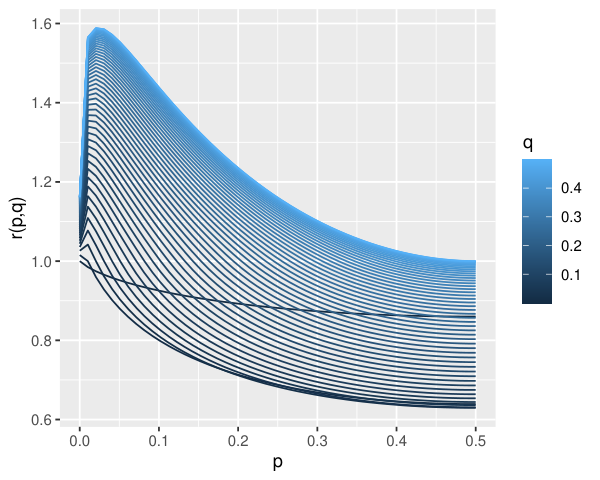
Figure 5: Minimax lower bound in Theorem 3 (first row), lower bound of probability of success of the MLE algorithm in Theorem 4 (second row), and lower bound of probability of success of the polynomial-time algorithm (third row), for regular expander with n=64n=64, d=30d=30 (first column) and star graph with n=64n=64 (second column.) The x-axis indicates p∈[0,12]p\in[0,\frac{1}{2}]. Different blue colors represent different q∈[0,12]q\in[0,\frac{1}{2}]. Red dashed lines denote the bounds provided in Section 3 for corresponding graphs.

Figure 5 graphically illustrates the bounds of the probabilities in Theorem 3 and 4, and the lower bound of the probability of success of the polynomial-time algorithm (which is 1−ϵ1−ϵ21-\epsilon_{1}-\epsilon_{2}) for the regular expanders and star graphs. Results for more classes of graphs are given in Appendix A.11.

As in Section 3.3, we can observe the gap between the fundamental limits and the performance of the polynomial-time algorithm in regular expanders. We can observe that the lower bound of the probability of success of the MLE algorithm increases as qq decreases, while the lower bound of the probability of success of the polynomial-time algorithm is always zero even with q=0q=0.

Next, we can observe that the value of qq has a substantial influence on the probability of exact recovery. When qq is close to 12\frac{1}{2}, exact recovery is impossible for any algorithm in star graphs for most pp values, as shown in the plot of minimax lower bounds. On the other hand, when qq is close to zero, the minimax lower bounds become zero in both of regular expanders and star graphs, that is, the necessary condition for exact recovery holds for any algorithm. Also, when qq is close to zero in regular expanders, the lower bound of the probability of success of the MLE algorithm becomes slightly higher than that in the regime where only the noisy edge observation XX is given.

Lastly, we remark that there is room for improvement in the lower bound of the probability of success of the MLE algorithm, because the bound decreases when pp decreases around zero in regular expanders. This does not match with the intuition that the probability of success must increase as pp decreases.

5 Concluding Remarks

We discussed the fundamental limits of the exact inference problem under a simple generative model assumption (Globerson et al. 2015), and considered two regimes, one in which only noisy edge observations are given, and one regime in which noisy edge and node observations are both provided. From the limit bounds, we derived the sufficient and necessary conditions for exact recovery irrespective of computational efficiency, and we further revealed that those conditions are tight up to at most a logarithmic factor. Moreover, by comparing the limit bounds of the MLE algorithm and a polynomial-time algorithm (Bello and Honorio 2019), we showed that there is a gap between the fundamental limits and the performance of a currently existent and tractable algorithm for exact inference, and thus there is still a need to develop better algorithms.

We assumed a plain generative model in this paper. Our strategies of the proofs will be able to provide a guide to future works dealing with more complex models. For instance, as in Heidari et al. 2020, considering non-binary categorical labels would be interesting. Finally, as mentioned in the main text, there is still room for improvement in the bounds of probabilities we derived.

References

  • Abbe (2017) Emmanuel Abbe. Community detection and stochastic block models: recent developments. The Journal of Machine Learning Research, 18(1):6446–6531, 2017.
  • Abbe et al. (2014) Emmanuel Abbe, Afonso S Bandeira, Annina Bracher, and Amit Singer. Decoding binary node labels from censored edge measurements: Phase transition and efficient recovery. IEEE Transactions on Network Science and Engineering, 1(1):10–22, 2014.
  • Banks et al. (2016) Jess Banks, Cristopher Moore, Joe Neeman, and Praneeth Netrapalli. Information-theoretic thresholds for community detection in sparse networks. In Conference on Learning Theory, pages 383–416, 2016.
  • Bello and Honorio (2019) Kevin Bello and Jean Honorio. Exact inference in structured prediction. In Advances in Neural Information Processing Systems, pages 3698–3707, 2019.
  • Bickel and Doksum (2015) Peter J Bickel and Kjell A Doksum. Mathematical statistics: basic ideas and selected topics, volume I, volume 117. CRC Press, 2015.
  • Bollobás (2013) Béla Bollobás. Modern graph theory, volume 184. Springer Science & Business Media, 2013.
  • Boucheron et al. (2013) Stéphane Boucheron, Gábor Lugosi, and Pascal Massart. Concentration inequalities: A nonasymptotic theory of independence. Oxford university press, 2013.
  • Chandrasekaran et al. (2008) Venkat Chandrasekaran, Nathan Srebro, and Prahladh Harsha. Complexity of inference in graphical models. In Proceedings of the Twenty-Fourth Conference on Uncertainty in Artificial Intelligence, UAI’08, page 70–78, Arlington, Virginia, USA, 2008. AUAI Press. ISBN 0974903949.
  • Chen and Xu (2014) Yudong Chen and Jiaming Xu. Statistical-computational phase transitions in planted models: The high-dimensional setting. In International Conference on Machine Learning, pages 244–252, 2014.
  • Chen et al. (2016) Yuxin Chen, Changho Suh, and Andrea J Goldsmith. Information recovery from pairwise measurements. IEEE Transactions on Information Theory, 62(10):5881–5905, 2016.
  • Cover (1999) Thomas M Cover. Elements of information theory. John Wiley & Sons, 1999.
  • Fortunato (2010) Santo Fortunato. Community detection in graphs. Physics reports, 486(3-5):75–174, 2010.
  • Foster et al. (2018) Dylan Foster, Karthik Sridharan, and Daniel Reichman. Inference in sparse graphs with pairwise measurements and side information. In International Conference on Artificial Intelligence and Statistics, pages 1810–1818. PMLR, 2018.
  • Globerson et al. (2015) Amir Globerson, Tim Roughgarden, David Sontag, and Cafer Yildirim. How hard is inference for structured prediction? In International Conference on Machine Learning, pages 2181–2190, 2015.
  • Heidari et al. (2020) Alireza Heidari, Ihab F Ilyas, and Theodoros Rekatsinas. Approximate inference in structured instances with noisy categorical observations. In Uncertainty in Artificial Intelligence, pages 412–421. PMLR, 2020.
  • Lafferty et al. (2001) John Lafferty, Andrew McCallum, and Fernando CN Pereira. Conditional random fields: Probabilistic models for segmenting and labeling sequence data. 2001.
  • Taskar et al. (2004) Ben Taskar, Carlos Guestrin, and Daphne Koller. Max-margin markov networks. In Advances in neural information processing systems, pages 25–32, 2004.
  • Tsochantaridis et al. (2005) Ioannis Tsochantaridis, Thorsten Joachims, Thomas Hofmann, and Yasemin Altun. Large margin methods for structured and interdependent output variables. Journal of machine learning research, 6(Sep):1453–1484, 2005.
  • Yu (1997) Bin Yu. Assouad, fano, and le cam. In Festschrift for Lucien Le Cam, pages 423–435. Springer, 1997.

Appendix A Supplementary Material

A.1 Preliminaries

We first introduce the notations, lemmas and facts which will be used throughout the proofs.

For any 𝒚∈𝒴={−1,1}n\boldsymbol{y}\in\mathcal{Y}=\{-1,1\}^{n}, we write Y:=𝒚​𝒚T=−𝒚​(−𝒚)TY:=\boldsymbol{y}\boldsymbol{y}^{T}=-\boldsymbol{y}(-\boldsymbol{y})^{T}. Also, for any n×nn\times n matrix AA and any subset ℬ⊆ℰ\mathcal{B}\subseteq\mathcal{E}, we denote by AℬA_{\mathcal{B}} an upper triangular matrix such that [Aℬ]i​j=Ai​j[A_{\mathcal{B}}]_{ij}=A_{ij} if (i,j)∈ℬ(i,j)\in\mathcal{B} and [Aℬ]i​j=0[A_{\mathcal{B}}]_{ij}=0 otherwise. We define 𝒴ℬ:={Yℬ;Y=𝒚​𝒚T,𝒚∈𝒴}\mathcal{Y}_{\mathcal{B}}:=\{Y_{\mathcal{B}}~;~Y=\boldsymbol{y}\boldsymbol{y}^{T},\boldsymbol{y}\in\mathcal{Y}\} for any ℬ⊆ℰ\mathcal{B}\subseteq\mathcal{E}.

We note that every connected graph has a spanning tree subgraph, which is a tree containing every vertex of the graph (Bollobás 2013). From this fact, we can prove the following lemma.

Lemma 1.

For any spanning tree subgraph 𝒢1=(𝒱,ℰ1)\mathcal{G}_{1}=(\mathcal{V},\mathcal{E}_{1}) of a connected graph 𝒢=(𝒱,ℰ)\mathcal{G}=(\mathcal{V},\mathcal{E}) with nn nodes, the map (Yℰ∈𝒴ℰ)↦([Yℰ]ℰ1=Yℰ1∈𝒴ℰ1)(Y_{\mathcal{E}}\in\mathcal{Y}_{\mathcal{E}})\mapsto([Y_{\mathcal{E}}]_{\mathcal{E}_{1}}=Y_{\mathcal{E}_{1}}\in\mathcal{Y}_{\mathcal{E}_{1}}) is bijective. This implies that the elements of Yℰ2Y_{\mathcal{E}_{2}} can be determined by the elements of Yℰ1Y_{\mathcal{E}_{1}} where ℰ2=ℰ\ℰ1\mathcal{E}_{2}=\mathcal{E}\backslash\mathcal{E}_{1}.

Proof.

For any Yℰ1∈𝒴ℰ1Y_{\mathcal{E}_{1}}\in\mathcal{Y}_{\mathcal{E}_{1}}, there exists Yℰ∈𝒴ℰY_{\mathcal{E}}\in\mathcal{Y}_{\mathcal{E}} such that [Yℰ]ℰ1=Yℰ1[Y_{\mathcal{E}}]_{\mathcal{E}_{1}}=Y_{\mathcal{E}_{1}}, i.e., the map is onto. Also, for any connected graph 𝒢=(𝒱,ℰ)\mathcal{G}=(\mathcal{V},\mathcal{E}), 𝒚​𝒚T=−𝒚​(−𝒚)T\boldsymbol{y}\boldsymbol{y}^{T}=-\boldsymbol{y}(-\boldsymbol{y})^{T} for all 𝒚∈𝒴\boldsymbol{y}\in\mathcal{Y} and (𝒚​𝒚T)ℰ≠(𝒚~​𝒚~T)ℰ\big(\boldsymbol{y}\boldsymbol{y}^{T}\big)_{\mathcal{E}}\neq\big(\tilde{\boldsymbol{y}}\tilde{\boldsymbol{y}}^{T}\big)_{\mathcal{E}} if 𝒚~≠𝒚\tilde{\boldsymbol{y}}\neq\boldsymbol{y} or −𝒚-\boldsymbol{y}, and thus the cardinality of 𝒴ℰ\mathcal{Y}_{\mathcal{E}} is |𝒴ℰ|=12⋅|𝒴|=2n−1|\mathcal{Y}_{\mathcal{E}}|=\frac{1}{2}\cdot|\mathcal{Y}|=2^{n-1}. This holds for both 𝒴ℰ\mathcal{Y}_{\mathcal{E}} and 𝒴ℰ1\mathcal{Y}_{\mathcal{E}_{1}}, that is, they have the same cardinality. Therefore, the map is bijective. ∎

The above lemma results in the following fact:

Fact 1.

Note that for any spanning tree subgraph 𝒢1=(𝒱,ℰ1)\mathcal{G}_{1}=(\mathcal{V},\mathcal{E}_{1}) of a connected graph 𝒢=(𝒱,ℰ)\mathcal{G}=(\mathcal{V},\mathcal{E}) with nn nodes, the cardinaltiy of ℰ1\mathcal{E}_{1} is |ℰ1|=n−1|\mathcal{E}_{1}|=n-1 and |𝒴ℰ1|=2n−1|\mathcal{Y}_{\mathcal{E}_{1}}|=2^{n-1}. Thus, we derive that 𝒴ℰ1={−1,1}n−1\mathcal{Y}_{\mathcal{E}_{1}}=\{-1,1\}^{n-1}.

Next, for any 𝒚\boldsymbol{y} and 𝒚′∈𝒴\boldsymbol{y}^{\prime}\in\mathcal{Y}, we define S𝒚′​(𝒚):={i∈𝒱;yi′≠yi}S_{\boldsymbol{y}^{\prime}}(\boldsymbol{y}):=\{i\in\mathcal{V}~;~y^{\prime}_{i}\neq y_{i}\}. We denote the Hamming distance by d⁡(⋅,⋅)d(\cdot,\cdot). Now, we can easily check the following facts:

Fact 2.

d((𝒚′𝒚′T)ℰ,(𝒚𝒚T)ℰ)=∑(i,j)∈ℰ𝕀[yi′yj′≠yiyj]=|ℰ(S𝒚′(𝒚),S𝒚′(𝒚)c)|d\Big((\boldsymbol{y}^{\prime}{\boldsymbol{y}^{\prime}}^{T})_{\mathcal{E}},(\boldsymbol{y}{\boldsymbol{y}}^{T})_{\mathcal{E}}\Big)=\sum_{(i,j)\in\mathcal{E}}\mathbb{I}[y^{\prime}_{i}y^{\prime}_{j}\neq y_{i}y_{j}]=\big|\mathcal{E}\big(S_{\boldsymbol{y}^{\prime}}(\boldsymbol{y}),S_{\boldsymbol{y}^{\prime}}(\boldsymbol{y})^{c}\big)\big|.

Fact 3.

d(𝒚′,𝒚)=∑i∈𝒱𝕀[yi′≠yi]=|S𝒚′(𝒚)|d(\boldsymbol{y}^{\prime},\boldsymbol{y})=\sum_{i\in\mathcal{V}}\mathbb{I}[y^{\prime}_{i}\neq y_{i}]=|S_{\boldsymbol{y}^{\prime}}(\boldsymbol{y})|.

Fact 4.

For a fixed 𝐲′\boldsymbol{y}^{\prime}, the map S𝐲′​(⋅):𝐲∈𝒴↦S𝐲′​(𝐲)∈𝒫⁡(𝒱)S_{\boldsymbol{y}^{\prime}}(\cdot):\boldsymbol{y}\in\mathcal{Y}\mapsto S_{\boldsymbol{y}^{\prime}}(\boldsymbol{y})\in\mathcal{P}(\mathcal{V}) is bijective where 𝒫⁡(𝒱)\mathcal{P}(\mathcal{V}) is the power set of 𝒱\mathcal{V}.

Lastly, we present Assouad’s lemma (Lemma 2 in (Yu 1997)) and Lemma 3 which will be used to prove Lemma 4 and Lemma 6.

Lemma 2 (Assouad’s lemma).

Consider a distance function δ⁡(⋅,⋅)\delta(\cdot,\cdot) on 𝒴×𝒴\mathcal{Y}\times\mathcal{Y}. Suppose that there are nn pseudo-distances {δj​(⋅,⋅)}j=1,⋯,n\{\delta_{j}(\cdot,\cdot)\}_{j=1,\cdots,n} such that for any 𝐲,𝐲′∈𝒴\boldsymbol{y},\boldsymbol{y}^{\prime}\in\mathcal{Y},

δ⁡(𝒚,𝒚′)=∑j=1nδj​(𝒚,𝒚′)\delta(\boldsymbol{y},\boldsymbol{y}^{\prime})=\sum_{j=1}^{n}\delta_{j}(\boldsymbol{y},\boldsymbol{y}^{\prime})

and there exists αn>0\alpha_{n}>0 such that for all j=1,⋯,nj=1,\cdots,n,

δj​(𝒚,𝒚′)≥αn\delta_{j}(\boldsymbol{y},\boldsymbol{y}^{\prime})\geq\alpha_{n}

when yj≠yj′y_{j}\neq y^{\prime}_{j} and yi=yi′y_{i}=y^{\prime}_{i} for ∀i≠j\forall i\neq j. Let PX|𝐲P_{X|\boldsymbol{y}} be the conditional probability distribution of X∈𝒳X\in\mathcal{X} given 𝐲\boldsymbol{y}, and let p⁡(X|𝐲)p(X|\boldsymbol{y}) be its related probability mass function. Then for any estimator 𝐲^​(⋅)\hat{\boldsymbol{y}}(\cdot), we have

max𝒚∗∈𝒴𝔼X|𝒚∗[δ(𝒚^(X),𝒚∗)]≥n⋅αn2min{∥PX|𝒚∧PX|𝒚′∥:∑i=1n𝕀[yi≠yi′]=1,𝒚,𝒚′∈𝒴}\underset{\boldsymbol{y}^{*}\in\mathcal{Y}}{\max}~\mathbb{E}_{X|\boldsymbol{y}^{*}}\big[\delta(\hat{\boldsymbol{y}}(X),\boldsymbol{y}^{*})\big]\geq n\cdot\frac{\alpha_{n}}{2}\min\bigg\{\|P_{X|\boldsymbol{y}}\wedge P_{X|\boldsymbol{y}^{\prime}}\|:\sum_{i=1}^{n}\mathbb{I}[y_{i}\neq y^{\prime}_{i}]=1,~\boldsymbol{y},\boldsymbol{y}^{\prime}\in\mathcal{Y}\bigg\}

where ‖PX|𝐲∧PX|𝐲′‖=∑X∈𝒳p⁡(X|𝐲)∧p⁡(X|𝐲′)\|P_{X|\boldsymbol{y}}\wedge P_{X|\boldsymbol{y}^{\prime}}\|=\sum_{X\in\mathcal{X}}p(X|\boldsymbol{y})\wedge p(X|\boldsymbol{y}^{\prime}).

Lemma 3.

l⁡(n):=∑m=0n(nm)⁡[{pm⋅(1−p)n−m⋅q}∧{(1−p)m⋅pn−m⋅(1−q)}]l(n):=\sum_{m=0}^{n}\binom{n}{m}\Big[\big\{p^{m}\cdot(1-p)^{n-m}\cdot q\big\}\wedge\big\{(1-p)^{m}\cdot p^{n-m}\cdot(1-q)\big\}\Big], n∈ℕn\in\mathbb{N}, is a non-increasing function for any p,q∈[0,1]p,q\in[0,1].

Proof.

For any n≥1n\geq 1,

l⁡(n)\displaystyle l(n) =∑m=0n(nm)⁡[{pm⋅(1−p)n−m⋅q}∧{(1−p)m⋅pn−m⋅(1−q)}]\displaystyle=\sum_{m=0}^{n}\binom{n}{m}\Big[\big\{p^{m}\cdot(1-p)^{n-m}\cdot q\big\}\wedge\big\{(1-p)^{m}\cdot p^{n-m}\cdot(1-q)\big\}\Big]
=∑m=0n−1(n−1m)⁡[{pm⋅(1−p)n−m⋅q}∧{(1−p)m⋅pn−m⋅(1−q)}]\displaystyle=\sum_{m=0}^{n-1}\binom{n-1}{m}\Big[\big\{p^{m}\cdot(1-p)^{n-m}\cdot q\big\}\wedge\big\{(1-p)^{m}\cdot p^{n-m}\cdot(1-q)\big\}\Big]
+∑m=1n(n−1m−1)[{pm⋅(1−p)n−m⋅q}∧{(1−p)m⋅pn−m⋅(1−q)}]\displaystyle~~~~+\sum_{m=1}^{n}\binom{n-1}{m-1}\Big[\big\{p^{m}\cdot(1-p)^{n-m}\cdot q\big\}\wedge\big\{(1-p)^{m}\cdot p^{n-m}\cdot(1-q)\big\}\Big]
=∑m=0n−1(n−1m)⁡[{pm⋅(1−p)n−1−m⋅q⁡(1−p)}∧{(1−p)m⋅pn−1−m⋅(1−q)​p}]\displaystyle=\sum_{m=0}^{n-1}\binom{n-1}{m}\Big[\big\{p^{m}\cdot(1-p)^{n-1-m}\cdot q(1-p)\big\}\wedge\big\{(1-p)^{m}\cdot p^{n-1-m}\cdot(1-q)p\big\}\Big]
+∑m=0n−1(n−1m)[{pm⋅(1−p)n−1−m⋅qp}∧{(1−p)m⋅pn−1−m⋅(1−q)(1−p)}]\displaystyle~~~~+\sum_{m=0}^{n-1}\binom{n-1}{m}\Big[\big\{p^{m}\cdot(1-p)^{n-1-m}\cdot qp\big\}\wedge\big\{(1-p)^{m}\cdot p^{n-1-m}\cdot(1-q)(1-p)\big\}\Big]
≤∑m=0n−1(n−1m)[{pm⋅(1−p)n−1−m⋅q(1−p)+pm⋅(1−p)n−1−m⋅qp}\displaystyle\leq\sum_{m=0}^{n-1}\binom{n-1}{m}\Big[\big\{p^{m}\cdot(1-p)^{n-1-m}\cdot q(1-p)+p^{m}\cdot(1-p)^{n-1-m}\cdot qp\big\}
∧{(1−p)m⋅pn−1−m⋅(1−q)p+(1−p)m⋅pn−1−m⋅(1−q)(1−p)}]\displaystyle~~~~~~~~~~~~~~~~~~~~~~~~\wedge\big\{(1-p)^{m}\cdot p^{n-1-m}\cdot(1-q)p+(1-p)^{m}\cdot p^{n-1-m}\cdot(1-q)(1-p)\big\}\Big]
=∑m=0n−1(n−1m)⁡[{pm⋅(1−p)n−1−m⋅q}∧{(1−p)m⋅pn−1−m⋅(1−q)}]\displaystyle=\sum_{m=0}^{n-1}\binom{n-1}{m}\Big[\big\{p^{m}\cdot(1-p)^{n-1-m}\cdot q\big\}\wedge\big\{(1-p)^{m}\cdot p^{n-1-m}\cdot(1-q)\big\}\Big]
=l⁡(n−1)\displaystyle=l(n-1)

where the inequality holds because a∧b+c∧d≤(a+c)∧(b+d)a\wedge b+c\wedge d\leq(a+c)\wedge(b+d). ∎

A.2 Proof of Theorem 1

We can prove Theorem 1 by showing the following lemmas:

Lemma 4.

Under the same conditions as in Theorem 1, we have inf𝐲^:𝒳→𝒴supP∈𝒫ℙ(𝐲∗,X)∼P[𝐲^(X)≠𝐲∗]≥f1.\underset{\hat{\boldsymbol{y}}:\mathcal{X}\to\mathcal{Y}}{\inf}\underset{P\in\mathcal{P}}{\sup}\mathbb{P}_{(\boldsymbol{y}^{*},X)\sim P}\big[\hat{\boldsymbol{y}}(X)\neq\boldsymbol{y}^{*}\big]\geq f_{1}.

Lemma 5.

Under the same conditions as in Theorem 1, we have inf𝐲^:𝒳→𝒴supP∈𝒫ℙ(𝐲∗,X)∼P[𝐲^(X)≠𝐲∗]≥max{g1,g1∗}.\underset{\hat{\boldsymbol{y}}:\mathcal{X}\to\mathcal{Y}}{\inf}\underset{P\in\mathcal{P}}{\sup}\mathbb{P}_{(\boldsymbol{y}^{*},X)\sim P}\big[\hat{\boldsymbol{y}}(X)\neq\boldsymbol{y}^{*}\big]\geq\max\{g_{1},g_{1}^{*}\}.

A.2.1 Proof of Lemma 4

We apply Lemma 2 to our problem. Here, we consider the zero-one distance δ(𝒚,𝒚′)=𝕀[𝒚≠𝒚′]\delta(\boldsymbol{y},\boldsymbol{y}^{\prime})=\mathbb{I}[\boldsymbol{y}\neq\boldsymbol{y}^{\prime}] and the pseudo-distance δj(𝒚,𝒚′)=1n𝕀[𝒚≠𝒚′]\delta_{j}(\boldsymbol{y},\boldsymbol{y}^{\prime})=\frac{1}{n}\mathbb{I}[\boldsymbol{y}\neq\boldsymbol{y}^{\prime}] for j=1,⋯,nj=1,\cdots,n. Then with αn=1n\alpha_{n}=\frac{1}{n}, we can derive that

max𝒚∗∈𝒴ℙX|𝒚∗[𝒚^(X)≠𝒚∗]≥12min{∥PX|𝒚∧PX|𝒚′∥:∑i=1n𝕀[yi≠yi′]=1,𝒚,𝒚′∈𝒴}.\underset{\boldsymbol{y}^{*}\in\mathcal{Y}}{\max}~\mathbb{P}_{X|\boldsymbol{y}^{*}}\big[\hat{\boldsymbol{y}}(X)\neq\boldsymbol{y}^{*}\big]\geq\frac{1}{2}\min\bigg\{\|P_{X|\boldsymbol{y}}\wedge P_{X|\boldsymbol{y}^{\prime}}\|:\sum_{i=1}^{n}\mathbb{I}[y_{i}\neq y^{\prime}_{i}]=1,~\boldsymbol{y},\boldsymbol{y}^{\prime}\in\mathcal{Y}\bigg\}.

To find the minimum value of the RHS, we consider 𝒚,𝒚′\boldsymbol{y},\boldsymbol{y}^{\prime} such that yk≠yk′y_{k}\neq y^{\prime}_{k} and yi=yi′y_{i}=y^{\prime}_{i} for ∀i≠k\forall i\neq k. Denote the set of edges which are connected to the kkth node by ℰk\mathcal{E}_{k}. Then we can obtain that

p⁡(X|𝒚)∧p⁡(X|𝒚′)\displaystyle p(X|\boldsymbol{y})\wedge p(X|\boldsymbol{y}^{\prime}) ={∏(i,j)∈ℰp⁡(Xi​j|yi​yj)}∧{∏(i,j)∈ℰp⁡(Xi​j|yi′​yj′)}\displaystyle=\bigg\{\prod_{(i,j)\in\mathcal{E}}p(X_{ij}|y_{i}y_{j})\bigg\}\wedge\bigg\{\prod_{(i,j)\in\mathcal{E}}p(X_{ij}|y^{\prime}_{i}y^{\prime}_{j})\bigg\}
={∏(i,j)∉ℰkp⁡(Xi​j|yi​yj)⋅∏(i,j)∈ℰkp⁡(Xi​j|yi​yj)}∧{∏(i,j)∉ℰkp⁡(Xi​j|yi​yj)⋅∏(i,j)∈ℰkp⁡(Xi​j|yi′​yj′)}\displaystyle=\bigg\{\prod_{(i,j)\notin\mathcal{E}_{k}}p(X_{ij}|y_{i}y_{j})\cdot\prod_{(i,j)\in\mathcal{E}_{k}}p(X_{ij}|y_{i}y_{j})\bigg\}\wedge\bigg\{\prod_{(i,j)\notin\mathcal{E}_{k}}p(X_{ij}|y_{i}y_{j})\cdot\prod_{(i,j)\in\mathcal{E}_{k}}p(X_{ij}|y^{\prime}_{i}y^{\prime}_{j})\bigg\}
={∏(i,j)∉ℰkp⁡(Xi​j|yi​yj)}×[{∏(i,j)∈ℰkp⁡(Xi​j|yi​yj)}∧{∏(i,j)∈ℰkp⁡(Xi​j|yi′​yj′)}]\displaystyle=\bigg\{\prod_{(i,j)\notin\mathcal{E}_{k}}p(X_{ij}|y_{i}y_{j})\bigg\}\times\Bigg[\bigg\{\prod_{(i,j)\in\mathcal{E}_{k}}p(X_{ij}|y_{i}y_{j})\bigg\}\wedge\bigg\{\prod_{(i,j)\in\mathcal{E}_{k}}p(X_{ij}|y^{\prime}_{i}y^{\prime}_{j})\bigg\}\Bigg]
={∏(i,j)∉ℰkp⁡(Xi​j|yi​yj)}×[{∏(i,j)∈ℰkp⁡(Xi​j|yi​yj)}∧{∏(i,j)∈ℰk1−p⁡(Xi​j|yi​yj)}]\displaystyle=\bigg\{\prod_{(i,j)\notin\mathcal{E}_{k}}p(X_{ij}|y_{i}y_{j})\bigg\}\times\Bigg[\bigg\{\prod_{(i,j)\in\mathcal{E}_{k}}p(X_{ij}|y_{i}y_{j})\bigg\}\wedge\bigg\{\prod_{(i,j)\in\mathcal{E}_{k}}1-p(X_{ij}|y_{i}y_{j})\bigg\}\Bigg]
={∏(i,j)∉ℰkp⁡(Xi​j|yi​yj)}\displaystyle=\bigg\{\prod_{(i,j)\notin\mathcal{E}_{k}}p(X_{ij}|y_{i}y_{j})\bigg\}
×[{pd⁡(Xℰk,Yℰk)⋅(1−p)Δk−d⁡(Xℰk,Yℰk)}∧{(1−p)d⁡(Xℰk,Yℰk)⋅pΔk−d⁡(Xℰk,Yℰk)}].\displaystyle~~~\times\Bigg[\bigg\{p^{d(X_{\mathcal{E}_{k}},Y_{\mathcal{E}_{k}})}\cdot(1-p)^{\Delta_{k}-d(X_{\mathcal{E}_{k}},Y_{\mathcal{E}_{k}})}\bigg\}\wedge\bigg\{(1-p)^{d(X_{\mathcal{E}_{k}},Y_{\mathcal{E}_{k}})}\cdot p^{\Delta_{k}-d(X_{\mathcal{E}_{k}},Y_{\mathcal{E}_{k}})}\bigg\}\Bigg].

Accordingly,

‖PX|𝒚∧PX|𝒚′‖\displaystyle\|P_{X|\boldsymbol{y}}\wedge P_{X|\boldsymbol{y}^{\prime}}\| =∑X∈𝒳p⁡(X|𝒚)∧p⁡(X|𝒚′)\displaystyle=\sum_{X\in\mathcal{X}}p(X|\boldsymbol{y})\wedge p(X|\boldsymbol{y}^{\prime})
=∑X∈𝒳{∏(i,j)∉ℰkp⁡(Xi​j|yi​yj)}\displaystyle=\sum_{X\in\mathcal{X}}\bigg\{\prod_{(i,j)\notin\mathcal{E}_{k}}p(X_{ij}|y_{i}y_{j})\bigg\}
×[{pd⁡(Xℰk,Yℰk)⋅(1−p)Δk−d⁡(Xℰk,Yℰk)}∧{(1−p)d⁡(Xℰk,Yℰk)⋅pΔk−d⁡(Xℰk,Yℰk)}]\displaystyle~~~~~~~~~~\times\Bigg[\bigg\{p^{d(X_{\mathcal{E}_{k}},Y_{\mathcal{E}_{k}})}\cdot(1-p)^{\Delta_{k}-d(X_{\mathcal{E}_{k}},Y_{\mathcal{E}_{k}})}\bigg\}\wedge\bigg\{(1-p)^{d(X_{\mathcal{E}_{k}},Y_{\mathcal{E}_{k}})}\cdot p^{\Delta_{k}-d(X_{\mathcal{E}_{k}},Y_{\mathcal{E}_{k}})}\bigg\}\Bigg]
=∑Xi​j∈{−1,1}(i,j)∉ℰk{∏(i,j)∉ℰkp⁡(Xi​j|yi​yj)}\displaystyle=\mathop{\sum_{X_{ij}\in\{-1,1\}}}_{(i,j)\notin\mathcal{E}_{k}}\bigg\{\prod_{(i,j)\notin\mathcal{E}_{k}}p(X_{ij}|y_{i}y_{j})\bigg\}
×∑Xi​j∈{−1,1}(i,j)∈ℰk[{pd⁡(Xℰk,Yℰk)⋅(1−p)Δk−d⁡(Xℰk,Yℰk)}∧{(1−p)d⁡(Xℰk,Yℰk)⋅pΔk−d⁡(Xℰk,Yℰk)}]\displaystyle~~~~\times\mathop{\sum_{X_{ij}\in\{-1,1\}}}_{(i,j)\in\mathcal{E}_{k}}\Bigg[\bigg\{p^{d(X_{\mathcal{E}_{k}},Y_{\mathcal{E}_{k}})}\cdot(1-p)^{\Delta_{k}-d(X_{\mathcal{E}_{k}},Y_{\mathcal{E}_{k}})}\bigg\}\wedge\bigg\{(1-p)^{d(X_{\mathcal{E}_{k}},Y_{\mathcal{E}_{k}})}\cdot p^{\Delta_{k}-d(X_{\mathcal{E}_{k}},Y_{\mathcal{E}_{k}})}\bigg\}\Bigg]
=∑Xi​j∈{−1,1}(i,j)∈ℰk[{pd⁡(Xℰk,Yℰk)⋅(1−p)Δk−d⁡(Xℰk,Yℰk)}∧{(1−p)d⁡(Xℰk,Yℰk)⋅pΔk−d⁡(Xℰk,Yℰk)}].\displaystyle=\mathop{\sum_{X_{ij}\in\{-1,1\}}}_{(i,j)\in\mathcal{E}_{k}}\Bigg[\bigg\{p^{d(X_{\mathcal{E}_{k}},Y_{\mathcal{E}_{k}})}\cdot(1-p)^{\Delta_{k}-d(X_{\mathcal{E}_{k}},Y_{\mathcal{E}_{k}})}\bigg\}\wedge\bigg\{(1-p)^{d(X_{\mathcal{E}_{k}},Y_{\mathcal{E}_{k}})}\cdot p^{\Delta_{k}-d(X_{\mathcal{E}_{k}},Y_{\mathcal{E}_{k}})}\bigg\}\Bigg].

Note that d⁡(Xℰk,Yℰk)d(X_{\mathcal{E}_{k}},Y_{\mathcal{E}_{k}}) has a value between 00 and Δk\Delta_{k}, and for each m∈[0,Δk]m\in[0,\Delta_{k}], there exist (Δkm)\binom{\Delta_{k}}{m} different XℰkX_{\mathcal{E}_{k}}’s satisfying d⁡(Xℰk,Yℰk)=md(X_{\mathcal{E}_{k}},Y_{\mathcal{E}_{k}})=m. Hence, we can write that

‖PX|𝒚∧PX|𝒚′‖\displaystyle\|P_{X|\boldsymbol{y}}\wedge P_{X|\boldsymbol{y}^{\prime}}\| =∑m=0Δk(Δkm)⁡[{pm⋅(1−p)Δk−m}∧{(1−p)m⋅pΔk−m}],\displaystyle=\sum_{m=0}^{\Delta_{k}}\binom{\Delta_{k}}{m}\bigg[\Big\{p^{m}\cdot(1-p)^{\Delta_{k}-m}\Big\}\wedge\Big\{(1-p)^{m}\cdot p^{\Delta_{k}-m}\Big\}\bigg],

and consequently,

min{∥PX|𝒚∧PX|𝒚′∥:∑i=1n𝕀[yi≠yi′]=1,𝒚,𝒚′∈𝒴}\displaystyle\min\bigg\{\|P_{X|\boldsymbol{y}}\wedge P_{X|\boldsymbol{y}^{\prime}}\|:\sum_{i=1}^{n}\mathbb{I}[y_{i}\neq y^{\prime}_{i}]=1,~\boldsymbol{y},\boldsymbol{y}^{\prime}\in\mathcal{Y}\bigg\}
=min1≤k≤n​(∑m=0Δk(Δkm)⁡[{pm⋅(1−p)Δk−m}∧{(1−p)m⋅pΔk−m}])\displaystyle=\underset{1\leq k\leq n}{\min}\Bigg(\sum_{m=0}^{\Delta_{k}}\binom{\Delta_{k}}{m}\bigg[\Big\{p^{m}\cdot(1-p)^{\Delta_{k}-m}\Big\}\wedge\Big\{(1-p)^{m}\cdot p^{\Delta_{k}-m}\Big\}\bigg]\Bigg)
=∑m=0Δmax(Δmaxm)⁡[{pm⋅(1−p)Δmax−m}∧{(1−p)m⋅pΔmax−m}].\displaystyle=\sum_{m=0}^{\Delta_{\max}}\binom{\Delta_{\max}}{m}\bigg[\Big\{p^{m}\cdot(1-p)^{\Delta_{\max}-m}\Big\}\wedge\Big\{(1-p)^{m}\cdot p^{\Delta_{\max}-m}\Big\}\bigg].

The last equality holds by Lemma 3, where qq is set as 12\frac{1}{2}.

Finally, consider a joint probability distribution P0P_{0} of 𝒚∗\boldsymbol{y}^{*} and XX where the marginal probability of 𝒚∗\boldsymbol{y}^{*} is p𝒚∗​(𝒚0)=1p_{\boldsymbol{y}^{*}}(\boldsymbol{y}_{0})=1 for some 𝒚0∈𝒴\boldsymbol{y}_{0}\in\mathcal{Y}, and where XX given 𝒚∗\boldsymbol{y}^{*} follows the assumed conditional probability distribution. Then we have that

supP∈𝒫ℙ(𝒚∗,X)∼P[𝒚^(X)≠𝒚∗]\displaystyle\underset{P\in\mathcal{P}}{\sup}\mathbb{P}_{(\boldsymbol{y}^{*},X)\sim P}\big[\hat{\boldsymbol{y}}(X)\neq\boldsymbol{y}^{*}\big] ≥ℙ(𝒚∗,X)∼P0[𝒚^(X)≠𝒚∗]\displaystyle\geq\mathbb{P}_{(\boldsymbol{y}^{*},X)\sim P_{0}}\big[\hat{\boldsymbol{y}}(X)\neq\boldsymbol{y}^{*}\big]
=ℙX|𝒚0[𝒚^(X)≠𝒚0]\displaystyle=\mathbb{P}_{X|\boldsymbol{y}_{0}}\big[\hat{\boldsymbol{y}}(X)\neq\boldsymbol{y}_{0}\big]

which holds for any 𝒚0∈𝒴\boldsymbol{y}_{0}\in\mathcal{Y}. Hence, we derive that

supP∈𝒫ℙ(𝒚∗,X)∼P[𝒚^(X)≠𝒚∗]≥max𝒚∗∈𝒴ℙX|𝒚∗[𝒚^(X)≠𝒚∗]\underset{P\in\mathcal{P}}{\sup}\mathbb{P}_{(\boldsymbol{y}^{*},X)\sim P}\big[\hat{\boldsymbol{y}}(X)\neq\boldsymbol{y}^{*}\big]\geq\underset{\boldsymbol{y}^{*}\in\mathcal{Y}}{\max}~\mathbb{P}_{X|\boldsymbol{y}^{*}}\big[\hat{\boldsymbol{y}}(X)\neq\boldsymbol{y}^{*}\big]

for any estimator 𝒚^​(⋅)\hat{\boldsymbol{y}}(\cdot).

Therefore, we have

inf𝒚^:𝒳→𝒴supP∈𝒫ℙ(𝒚∗,X)∼P[𝒚^(X)≠𝒚∗]\displaystyle\underset{\hat{\boldsymbol{y}}:\mathcal{X}\to\mathcal{Y}}{\inf}\underset{P\in\mathcal{P}}{\sup}\mathbb{P}_{(\boldsymbol{y}^{*},X)\sim P}\big[\hat{\boldsymbol{y}}(X)\neq\boldsymbol{y}^{*}\big] ≥12min{∥PX|𝒚∧PX|𝒚′∥:∑i=1n𝕀[yi≠yi′]=1,𝒚,𝒚′∈𝒴}\displaystyle\geq\frac{1}{2}\min\bigg\{\|P_{X|\boldsymbol{y}}\wedge P_{X|\boldsymbol{y}^{\prime}}\|:\sum_{i=1}^{n}\mathbb{I}[y_{i}\neq y^{\prime}_{i}]=1,~\boldsymbol{y},\boldsymbol{y}^{\prime}\in\mathcal{Y}\bigg\}
=12​∑m=0Δmax(Δmaxm)⁡[{pm⋅(1−p)Δmax−m}∧{(1−p)m⋅pΔmax−m}]=f1.\displaystyle=\frac{1}{2}\sum_{m=0}^{\Delta_{\max}}\binom{\Delta_{\max}}{m}\bigg[\Big\{p^{m}\cdot(1-p)^{\Delta_{\max}-m}\Big\}\wedge\Big\{(1-p)^{m}\cdot p^{\Delta_{\max}-m}\Big\}\bigg]=f_{1}.

A.2.2 Proof of Lemma 5

We will apply Fano’s inequality (Theorem 2.10.1 in (Cover 1999)) to our problem. When we observe that 𝒚∗→X→𝒚^\boldsymbol{y}^{*}\rightarrow X\rightarrow\hat{\boldsymbol{y}} forms a Markov chain, we have

ℙ⁡(𝒚^≠𝒚∗)≥1−𝕀⁡(𝒚∗,X)+log⁡2log⁡|𝒴|\mathbb{P}(\hat{\boldsymbol{y}}\neq\boldsymbol{y}^{*})\geq 1-\frac{\mathbb{I}(\boldsymbol{y}^{*},X)+\log 2}{\log|\mathcal{Y}|}

where 𝕀⁡(𝒚∗,X)\mathbb{I}(\boldsymbol{y}^{*},X) is the mutual information of 𝒚∗\boldsymbol{y}^{*} and XX. To achieve our goal, we need to find an exact form or an upper bound of the mutual information 𝕀⁡(𝒚∗,X)\mathbb{I}(\boldsymbol{y}^{*},X). For simplicity, we write 𝒚=𝒚∗\boldsymbol{y}=\boldsymbol{y}^{*} in the rest of the proof.

We can write the mutual information as follows:

𝕀⁡(𝒚,X)\displaystyle\mathbb{I}(\boldsymbol{y},X) =12n∑𝒚∈𝒴𝕂𝕃(PX|𝒚∥PX)\displaystyle=\frac{1}{2^{n}}\sum_{\boldsymbol{y}\in\mathcal{Y}}\mathbb{KL}(P_{X|\boldsymbol{y}}\|P_{X})
=12n​∑𝒚∈𝒴∑X∈𝒳p⁡(X|𝒚)​log⁡[p⁡(X|𝒚)p⁡(X)⋅q⁡(X)q⁡(X)]\displaystyle=\frac{1}{2^{n}}\sum_{\boldsymbol{y}\in\mathcal{Y}}\sum_{X\in\mathcal{X}}p(X|\boldsymbol{y})\log\bigg[\frac{p(X|\boldsymbol{y})}{p(X)}\cdot\frac{q(X)}{q(X)}\bigg]
=12n​∑𝒚∈𝒴∑X∈𝒳p⁡(X|𝒚)​[log⁡p⁡(X|𝒚)q⁡(X)−log⁡p⁡(X)q⁡(X)]\displaystyle=\frac{1}{2^{n}}\sum_{\boldsymbol{y}\in\mathcal{Y}}\sum_{X\in\mathcal{X}}p(X|\boldsymbol{y})\bigg[\log\frac{p(X|\boldsymbol{y})}{q(X)}-\log\frac{p(X)}{q(X)}\bigg]
=12n∑𝒚∈𝒴𝕂𝕃(PX|𝒚∥QX)−∑X∈𝒳[12n∑𝒚∈𝒴p(X|𝒚)]logp⁡(X)q⁡(X)\displaystyle=\frac{1}{2^{n}}\sum_{\boldsymbol{y}\in\mathcal{Y}}\mathbb{KL}(P_{X|\boldsymbol{y}}\|Q_{X})-\sum_{X\in\mathcal{X}}\bigg[\frac{1}{2^{n}}\sum_{\boldsymbol{y}\in\mathcal{Y}}p(X|\boldsymbol{y})\bigg]\log\frac{p(X)}{q(X)}
=12n∑𝒚∈𝒴𝕂𝕃(PX|𝒚∥QX)−∑X∈𝒳p(X)logp⁡(X)q⁡(X)\displaystyle=\frac{1}{2^{n}}\sum_{\boldsymbol{y}\in\mathcal{Y}}\mathbb{KL}(P_{X|\boldsymbol{y}}\|Q_{X})-\sum_{X\in\mathcal{X}}p(X)\log\frac{p(X)}{q(X)}
=12n∑𝒚∈𝒴𝕂𝕃(PX|𝒚∥QX)−𝕂𝕃(PX∥QX).\displaystyle=\frac{1}{2^{n}}\sum_{\boldsymbol{y}\in\mathcal{Y}}\mathbb{KL}(P_{X|\boldsymbol{y}}\|Q_{X})-\mathbb{KL}(P_{X}\|Q_{X}).

The first equality holds because 𝒚\boldsymbol{y} follows a uniform distribution, and the rest holds for any distribution QXQ_{X} on 𝒳\mathcal{X}. If we set QXQ_{X} to be a uniform distribution on 𝒳\mathcal{X}, i.e., q⁡(x)=2−|ℰ|q(x)=2^{-|\mathcal{E}|}, then we have

𝕂𝕃(PX|𝒚∥QX)\displaystyle\mathbb{KL}(P_{X|\boldsymbol{y}}\|Q_{X}) =∑X∈𝒳p⁡(X|𝒚)​log⁡p⁡(X|𝒚)2−|ℰ|\displaystyle=\sum_{X\in\mathcal{X}}p(X|\boldsymbol{y})\log\frac{p(X|\boldsymbol{y})}{2^{-|\mathcal{E}|}}
=∑X∈𝒳{∏(i,j)∈ℰp⁡(Xi​j|yi​yj)}⋅[log⁡(∏(i,j)∈ℰp⁡(Xi​j|yi​yj))+|ℰ|​log⁡2]\displaystyle=\sum_{X\in\mathcal{X}}\Big\{\prod_{(i,j)\in\mathcal{E}}p(X_{ij}|y_{i}y_{j})\Big\}\cdot\bigg[\log\Big(\prod_{(i,j)\in\mathcal{E}}p(X_{ij}|y_{i}y_{j})\Big)+|\mathcal{E}|\log 2\bigg]
=[∑(i,j)∈ℰ∑Xi​j∈{−1,1}p⁡(Xi​j|yi​yj)​log⁡(p⁡(Xi​j|yi​yj))]+|ℰ|log⁡2\displaystyle=\bigg[\sum_{(i,j)\in\mathcal{E}}\sum_{X_{ij}\in\{-1,1\}}p(X_{ij}|y_{i}y_{j})\log\Big(p(X_{ij}|y_{i}y_{j})\Big)\bigg]+|\mathcal{E}|\log 2
=|ℰ|​(p​log⁡p+(1−p)​log⁡(1−p))+|ℰ|log⁡2\displaystyle=|\mathcal{E}|\Big(p\log p+(1-p)\log(1-p)\Big)+|\mathcal{E}|\log 2
=−|ℰ|​H∗​(p)+|ℰ|​log⁡2\displaystyle=-|\mathcal{E}|H^{*}(p)+|\mathcal{E}|\log 2

and

𝕂𝕃(PX∥QX)\displaystyle\mathbb{KL}(P_{X}\|Q_{X}) =∑X∈𝒳p⁡(X)​log⁡p⁡(X)2−|ℰ|\displaystyle=\sum_{X\in\mathcal{X}}p(X)\log\frac{p(X)}{2^{-|\mathcal{E}|}}
=∑X∈𝒳p⁡(X)​log⁡p⁡(X)+|ℰ|log⁡2\displaystyle=\sum_{X\in\mathcal{X}}p(X)\log p(X)+|\mathcal{E}|\log 2
=−H⁡(X)+|ℰ|​log⁡2\displaystyle=-H(X)+|\mathcal{E}|\log 2

where H(X)=−∑X∈𝒳p(X)logp(X)H(X)=-\sum_{X\in\mathcal{X}}p(X)\log p(X) is the entropy of XX. Hence, we have the following exact form of the mutual information:

𝕀⁡(𝒚,X)=H⁡(X)−|ℰ|​H∗​(p).\mathbb{I}(\boldsymbol{y},X)=H(X)-|\mathcal{E}|H^{*}(p).

Note that the entropy of a discrete random variable is always positive and bounded above by the logarithm of the size of its domain, which implies that 0≤H⁡(X)≤|ℰ|​log⁡20\leq H(X)\leq|\mathcal{E}|\log 2 in our case. By using this fact, we can simply find the upper bound of the mutual information as follows:

𝕀⁡(𝒚,X)≤|ℰ|​(log⁡2−H∗​(p)).\mathbb{I}(\boldsymbol{y},X)\leq|\mathcal{E}|\big(\log 2-H^{*}(p)\big).

Then we have

ℙ⁡(𝒚^≠𝒚∗)\displaystyle\mathbb{P}(\hat{\boldsymbol{y}}\neq\boldsymbol{y}^{*}) ≥1−|ℰ|​(log⁡2−H∗​(p))+log⁡2n​log⁡2\displaystyle\geq 1-\frac{|\mathcal{E}|\big(\log 2-H^{*}(p)\big)+\log 2}{n\log 2}
=n−1n−|ℰ|n⋅(1−H∗​(p)log⁡2)=g1.\displaystyle=\frac{n-1}{n}-\frac{|\mathcal{E}|}{n}\cdot\bigg(1-\frac{H^{*}(p)}{\log 2}\bigg)=g_{1}. (7)

Now, we want to find another upper bound of H⁡(X)H(X) instead of |ℰ|​log⁡2|\mathcal{E}|\log 2. For this, we can first write the probability mass function p⁡(X)p(X) as follows:

p⁡(X)\displaystyle p(X) =∑𝒚∈𝒴p⁡(X|𝒚)​p​(𝒚)=12n​∑𝒚∈𝒴p⁡(X|𝒚)=12n​∑𝒚∈𝒴{∏(i,j)∈ℰp⁡(Xi​j|yi​yj)}\displaystyle=\sum_{\boldsymbol{y}\in\mathcal{Y}}p(X|\boldsymbol{y})p(\boldsymbol{y})=\frac{1}{2^{n}}\sum_{\boldsymbol{y}\in\mathcal{Y}}p(X|\boldsymbol{y})=\frac{1}{2^{n}}\sum_{\boldsymbol{y}\in\mathcal{Y}}\Big\{\prod_{(i,j)\in\mathcal{E}}p(X_{ij}|y_{i}y_{j})\Big\}
=12n∑𝒚∈𝒴{∏(i,j)∈ℰp𝕀[Xi​j≠yiyj](1−p)1−𝕀[Xi​j≠yiyj]}\displaystyle=\frac{1}{2^{n}}\sum_{\boldsymbol{y}\in\mathcal{Y}}\Big\{\prod_{(i,j)\in\mathcal{E}}p^{\mathbb{I}[X_{ij}\neq y_{i}y_{j}]}(1-p)^{1-\mathbb{I}[X_{ij}\neq y_{i}y_{j}]}\Big\}
=12n​∑𝒚∈𝒴{pd⁡(X,Yℰ)​(1−p)|ℰ|−d⁡(X,Yℰ)}\displaystyle=\frac{1}{2^{n}}\sum_{\boldsymbol{y}\in\mathcal{Y}}\Big\{p^{d(X,Y_{\mathcal{E}})}(1-p)^{|\mathcal{E}|-d(X,Y_{\mathcal{E}})}\Big\}
=12n​(1−p)|ℰ|​∑𝒚∈𝒴(p1−p)d⁡(X,Yℰ).\displaystyle=\frac{1}{2^{n}}(1-p)^{|\mathcal{E}|}\sum_{\boldsymbol{y}\in\mathcal{Y}}\bigg(\frac{p}{1-p}\bigg)^{d(X,Y_{\mathcal{E}})}.

Here, we will partition the space 𝒳={−1,1}|ℰ|\mathcal{X}=\{-1,1\}^{|\mathcal{E}|} into 𝒴ℰ\mathcal{Y}_{\mathcal{E}} and 𝒳\𝒴ℰ\mathcal{X}\backslash\mathcal{Y}_{\mathcal{E}}, and deal with −∑X∈𝒴ℰp(X)logp(X)-\sum_{X\in\mathcal{Y}_{\mathcal{E}}}p(X)\log p(X) and −∑X∈𝒳\𝒴ℰp(X)logp(X)-\sum_{X\in\mathcal{X}\backslash\mathcal{Y}_{\mathcal{E}}}p(X)\log p(X) separately. The first thing to note is that 𝒴ℰ={Yℰ;Y=𝒚​𝒚T,𝒚∈𝒴}\mathcal{Y}_{\mathcal{E}}=\{Y_{\mathcal{E}}~;~Y=\boldsymbol{y}\boldsymbol{y}^{T},\boldsymbol{y}\in\mathcal{Y}\} is the set of all matrices whose elements are feasible label products of the edges. Therefore, if X∈𝒴ℰX\in\mathcal{Y}_{\mathcal{E}}, we can find a vector 𝒚′∈𝒴\boldsymbol{y}^{\prime}\in\mathcal{Y} which satisfies X=Yℰ′:=(𝒚′​𝒚′T)ℰX=Y^{\prime}_{\mathcal{E}}:=(\boldsymbol{y}^{\prime}{\boldsymbol{y}^{\prime}}^{T})_{\mathcal{E}}. On the other hand, if X∈𝒳\𝒴ℰX\in\mathcal{X}\backslash\mathcal{Y}_{\mathcal{E}}, there does not exist such a vector 𝒚′∈𝒴\boldsymbol{y}^{\prime}\in\mathcal{Y} satisfying X=Yℰ′:=(𝒚′​𝒚′T)ℰX=Y^{\prime}_{\mathcal{E}}:=(\boldsymbol{y}^{\prime}{\boldsymbol{y}^{\prime}}^{T})_{\mathcal{E}}.

First, consider the case that X∈𝒴ℰX\in\mathcal{Y}_{\mathcal{E}}. There exists 𝒚′∈𝒴\boldsymbol{y}^{\prime}\in\mathcal{Y} such that X=Yℰ′=(𝒚′​𝒚′T)ℰX=Y^{\prime}_{\mathcal{E}}=(\boldsymbol{y}^{\prime}{\boldsymbol{y}^{\prime}}^{T})_{\mathcal{E}}, and for each 𝒚∈𝒴\boldsymbol{y}\in\mathcal{Y}, we can write d⁡(X,Yℰ)=d⁡((𝒚′​𝒚′T)ℰ,(𝒚​𝒚T)ℰ)d(X,Y_{\mathcal{E}})=d\Big((\boldsymbol{y}^{\prime}{\boldsymbol{y}^{\prime}}^{T})_{\mathcal{E}},(\boldsymbol{y}{\boldsymbol{y}}^{T})_{\mathcal{E}}\Big). Hence, we have that

∑𝒚∈𝒴(p1−p)d⁡(X,Yℰ)\displaystyle\sum_{\boldsymbol{y}\in\mathcal{Y}}\bigg(\frac{p}{1-p}\bigg)^{d(X,Y_{\mathcal{E}})} =∑𝒚∈𝒴(p1−p)d⁡((𝒚′​𝒚′T)ℰ,(𝒚​𝒚T)ℰ)\displaystyle=\sum_{\boldsymbol{y}\in\mathcal{Y}}\bigg(\frac{p}{1-p}\bigg)^{d((\boldsymbol{y}^{\prime}{\boldsymbol{y}^{\prime}}^{T})_{\mathcal{E}},(\boldsymbol{y}{\boldsymbol{y}}^{T})_{\mathcal{E}})}
=∑𝒚∈𝒴(p1−p)|ℰ⁡(S𝒚′​(𝒚),S𝒚′​(𝒚)c)|\displaystyle=\sum_{\boldsymbol{y}\in\mathcal{Y}}\bigg(\frac{p}{1-p}\bigg)^{|\mathcal{E}(S_{\boldsymbol{y}^{\prime}}(\boldsymbol{y}),S_{\boldsymbol{y}^{\prime}}(\boldsymbol{y})^{c})|}
=∑S∈𝒫⁡(𝒱)(p1−p)|ℰ⁡(S,Sc)|=∑S⊆𝒱(p1−p)|ℰ⁡(S,Sc)|\displaystyle=\sum_{S\in\mathcal{P}(\mathcal{V})}\bigg(\frac{p}{1-p}\bigg)^{|\mathcal{E}(S,S^{c})|}=\sum_{S\subseteq\mathcal{V}}\bigg(\frac{p}{1-p}\bigg)^{|\mathcal{E}(S,S^{c})|}

where the second and third equalities hold by the Facts 2 and 4, respectively. Accordingly, for any X∈𝒴ℰX\in\mathcal{Y}_{\mathcal{E}},

p⁡(X)=12n​(1−p)|ℰ|​∑S⊆𝒱(p1−p)|ℰ⁡(S,Sc)|.p(X)=\frac{1}{2^{n}}(1-p)^{|\mathcal{E}|}\sum_{S\subseteq\mathcal{V}}\bigg(\frac{p}{1-p}\bigg)^{|\mathcal{E}(S,S^{c})|}.

Note that the above does not depend on XX. Also, |𝒴ℰ|=2n−1|\mathcal{Y}_{\mathcal{E}}|=2^{n-1} as shown in the proof of Lemma 1, thus

−∑X∈𝒴ℰp(X)logp(X)\displaystyle-\sum_{X\in\mathcal{Y}_{\mathcal{E}}}p(X)\log p(X) =−2n−1⋅12n(1−p)|ℰ|∑S⊆𝒱(p1−p)|ℰ⁡(S,Sc)|⋅log[12n(1−p)|ℰ|∑S⊆𝒱(p1−p)|ℰ⁡(S,Sc)|].\displaystyle=-2^{n-1}\cdot\frac{1}{2^{n}}(1-p)^{|\mathcal{E}|}\sum_{S\subseteq\mathcal{V}}\bigg(\frac{p}{1-p}\bigg)^{|\mathcal{E}(S,S^{c})|}\cdot\log\Bigg[\frac{1}{2^{n}}(1-p)^{|\mathcal{E}|}\sum_{S\subseteq\mathcal{V}}\bigg(\frac{p}{1-p}\bigg)^{|\mathcal{E}(S,S^{c})|}\Bigg].

Next, consider the case that X∈𝒳\𝒴ℰX\in\mathcal{X}\backslash\mathcal{Y}_{\mathcal{E}}. By the Fact 1, there exists 𝒚′∈𝒴\boldsymbol{y}^{\prime}\in\mathcal{Y} such that Xℰ1=Yℰ1′=(𝒚′​𝒚′T)ℰ1X_{\mathcal{E}_{1}}=Y^{\prime}_{\mathcal{E}_{1}}=(\boldsymbol{y}^{\prime}{\boldsymbol{y}^{\prime}}^{T})_{\mathcal{E}_{1}}. Also, since X∈𝒳\𝒴ℰX\in\mathcal{X}\backslash\mathcal{Y}_{\mathcal{E}}, we have that Xℰ2X_{\mathcal{E}_{2}} should not be equal to (𝒚′​𝒚′T)ℰ2(\boldsymbol{y}^{\prime}{\boldsymbol{y}^{\prime}}^{T})_{\mathcal{E}_{2}}. By using these facts and the triangle inequality, for each 𝒚∈𝒴\boldsymbol{y}\in\mathcal{Y}, we can derive the following:

d⁡(X,Yℰ)\displaystyle d(X,Y_{\mathcal{E}}) ≥|d⁡(Yℰ′,Yℰ)−d⁡(X,Yℰ′)|\displaystyle\geq|d(Y^{\prime}_{\mathcal{E}},Y_{\mathcal{E}})-d(X,Y^{\prime}_{\mathcal{E}})|
=|d⁡(Yℰ′,Yℰ)−d⁡(Xℰ2,Yℰ2′)|\displaystyle=|d(Y^{\prime}_{\mathcal{E}},Y_{\mathcal{E}})-d(X_{\mathcal{E}_{2}},Y^{\prime}_{\mathcal{E}_{2}})|
=||ℰ⁡(S𝒚′​(𝒚),S𝒚′​(𝒚)c)|−d⁡(Xℰ2,Yℰ2′)|.\displaystyle=\Big|\big|\mathcal{E}\big(S_{\boldsymbol{y}^{\prime}}(\boldsymbol{y}),S_{\boldsymbol{y}^{\prime}}(\boldsymbol{y})^{c}\big)\big|-d(X_{\mathcal{E}_{2}},Y^{\prime}_{\mathcal{E}_{2}})\Big|.

Therefore,

p⁡(X)\displaystyle p(X) =12n​(1−p)|ℰ|​∑𝒚∈𝒴(p1−p)d⁡(X,Yℰ)\displaystyle=\frac{1}{2^{n}}(1-p)^{|\mathcal{E}|}\sum_{\boldsymbol{y}\in\mathcal{Y}}\bigg(\frac{p}{1-p}\bigg)^{d(X,Y_{\mathcal{E}})}
≤12n​(1−p)|ℰ|​∑𝒚∈𝒴(p1−p)||ℰ⁡(S𝒚′​(𝒚),S𝒚′​(𝒚)c)|−d⁡(Xℰ2,Yℰ2′)|\displaystyle\leq\frac{1}{2^{n}}(1-p)^{|\mathcal{E}|}\sum_{\boldsymbol{y}\in\mathcal{Y}}\bigg(\frac{p}{1-p}\bigg)^{\big||\mathcal{E}(S_{\boldsymbol{y}^{\prime}}(\boldsymbol{y}),S_{\boldsymbol{y}^{\prime}}(\boldsymbol{y})^{c})|-d(X_{\mathcal{E}_{2}},Y^{\prime}_{\mathcal{E}_{2}})\big|}
=12n​(1−p)|ℰ|​∑S⊆𝒱(p1−p)||ℰ⁡(S,Sc)|−d⁡(Xℰ2,Yℰ2′)|\displaystyle=\frac{1}{2^{n}}(1-p)^{|\mathcal{E}|}\sum_{S\subseteq\mathcal{V}}\bigg(\frac{p}{1-p}\bigg)^{\big||\mathcal{E}(S,S^{c})|-d(X_{\mathcal{E}_{2}},Y^{\prime}_{\mathcal{E}_{2}})\big|}

where the inequality holds because p∈[0,12]p\in[0,\frac{1}{2}]. Now, note that −p​log⁡p-p\log p increases as pp grows from 00 to e−1e^{-1}. Also, we can see that

p⁡(X)\displaystyle p(X) ≤12n​(1−p)|ℰ|​∑S⊆𝒱(p1−p)||ℰ⁡(S,Sc)|−d⁡(Xℰ2,Yℰ2′)|\displaystyle\leq\frac{1}{2^{n}}(1-p)^{|\mathcal{E}|}\sum_{S\subseteq\mathcal{V}}\bigg(\frac{p}{1-p}\bigg)^{\big||\mathcal{E}(S,S^{c})|-d(X_{\mathcal{E}_{2}},Y^{\prime}_{\mathcal{E}_{2}})\big|}
≤12n​(1−p)|ℰ|​∑S⊆𝒱1=12n​(1−p)|ℰ|⋅2n=(1−p)|ℰ|.\displaystyle\leq\frac{1}{2^{n}}(1-p)^{|\mathcal{E}|}\sum_{S\subseteq\mathcal{V}}1=\frac{1}{2^{n}}(1-p)^{|\mathcal{E}|}\cdot 2^{n}=(1-p)^{|\mathcal{E}|}.

Hence, if we assume that (1−p)|ℰ|≤1e(1-p)^{|\mathcal{E}|}\leq\frac{1}{e}, we have

−p(X)logp(X)≤−12n(1−p)|ℰ|∑S⊆𝒱(p1−p)||ℰ⁡(S,Sc)|−d⁡(Xℰ2,Yℰ2′)|⋅log[12n(1−p)|ℰ|∑S⊆𝒱(p1−p)||ℰ⁡(S,Sc)|−d⁡(Xℰ2,Yℰ2′)|].-p(X)\log p(X)\leq-\frac{1}{2^{n}}(1-p)^{|\mathcal{E}|}\sum_{S\subseteq\mathcal{V}}\bigg(\frac{p}{1-p}\bigg)^{||\mathcal{E}(S,S^{c})|-d(X_{\mathcal{E}_{2}},Y^{\prime}_{\mathcal{E}_{2}})|}\cdot\log\Bigg[\frac{1}{2^{n}}(1-p)^{|\mathcal{E}|}\sum_{S\subseteq\mathcal{V}}\bigg(\frac{p}{1-p}\bigg)^{||\mathcal{E}(S,S^{c})|-d(X_{\mathcal{E}_{2}},Y^{\prime}_{\mathcal{E}_{2}})|}\Bigg].

We define ρ𝒢​(p,m):=∑S⊆𝒱(p1−p)||ℰ⁡(S,Sc)|−m|\rho_{\mathcal{G}}(p,m):=\sum_{S\subseteq\mathcal{V}}\big(\frac{p}{1-p}\big)^{||\mathcal{E}(S,S^{c})|-m|} and mX=d⁡(Xℰ2,Yℰ2′)m_{X}=d(X_{\mathcal{E}_{2}},Y^{\prime}_{\mathcal{E}_{2}}). We can check that mXm_{X} has a value between 11 and |ℰ2|=|ℰ|−n+1|\mathcal{E}_{2}|=|\mathcal{E}|-n+1 for any X∈𝒳\𝒴ℰX\in\mathcal{X}\backslash\mathcal{Y}_{\mathcal{E}}, and for each m∈[1,|ℰ|−n+1]m\in[1,|\mathcal{E}|-n+1], there exist (|ℰ|−n+1m)\binom{|\mathcal{E}|-n+1}{m} different Xℰ2X_{\mathcal{E}_{2}}’s satisfying mX=mm_{X}=m. Also, 2n−12^{n-1} different XX’s in 𝒳\𝒴ℰ\mathcal{X}\backslash\mathcal{Y}_{\mathcal{E}} have the same Xℰ2X_{\mathcal{E}_{2}}. In sum, for each m∈[1,|ℰ|−n+1]m\in[1,|\mathcal{E}|-n+1], there are 2n−1⋅(|ℰ|−n+1m)2^{n-1}\cdot\binom{|\mathcal{E}|-n+1}{m} different XX’s in 𝒳\𝒴ℰ\mathcal{X}\backslash\mathcal{Y}_{\mathcal{E}}. Therefore, we can derive that

−∑X∈𝒳\𝒴ℰp(X)logp(X)\displaystyle-\sum_{X\in\mathcal{X}\backslash\mathcal{Y}_{\mathcal{E}}}p(X)\log p(X) ≤−∑X∈𝒳\𝒴ℰ12n(1−p)|ℰ|ρ𝒢(p,mX)⋅log[12n(1−p)|ℰ|ρ𝒢(p,mX)]\displaystyle\leq-\sum_{X\in\mathcal{X}\backslash\mathcal{Y}_{\mathcal{E}}}\frac{1}{2^{n}}(1-p)^{|\mathcal{E}|}\rho_{\mathcal{G}}(p,m_{X})\cdot\log\bigg[\frac{1}{2^{n}}(1-p)^{|\mathcal{E}|}\rho_{\mathcal{G}}(p,m_{X})\bigg]
=−2n−1⋅∑m=1|ℰ|−n+1(|ℰ|−n+1m)12n(1−p)|ℰ|ρ𝒢(p,m)⋅log[12n(1−p)|ℰ|ρ𝒢(p,m)].\displaystyle=-2^{n-1}\cdot\sum_{m=1}^{|\mathcal{E}|-n+1}\binom{|\mathcal{E}|-n+1}{m}\frac{1}{2^{n}}(1-p)^{|\mathcal{E}|}\rho_{\mathcal{G}}(p,m)\cdot\log\bigg[\frac{1}{2^{n}}(1-p)^{|\mathcal{E}|}\rho_{\mathcal{G}}(p,m)\bigg].

Now we can find the upper bound of the entropy H⁡(X)H(X). Note that when m=0m=0,

(|ℰ|−n+10)​12n​(1−p)|ℰ|​ρ𝒢​(p,0)⋅log⁡[12n​(1−p)|ℰ|​ρ𝒢​(p,0)]\displaystyle\binom{|\mathcal{E}|-n+1}{0}\frac{1}{2^{n}}(1-p)^{|\mathcal{E}|}\rho_{\mathcal{G}}(p,0)\cdot\log\bigg[\frac{1}{2^{n}}(1-p)^{|\mathcal{E}|}\rho_{\mathcal{G}}(p,0)\bigg]
=12n​(1−p)|ℰ|​∑S⊆𝒱(p1−p)|ℰ⁡(S,Sc)|⋅log⁡[12n​(1−p)|ℰ|​∑S⊆𝒱(p1−p)|ℰ⁡(S,Sc)|].\displaystyle=\frac{1}{2^{n}}(1-p)^{|\mathcal{E}|}\sum_{S\subseteq\mathcal{V}}\bigg(\frac{p}{1-p}\bigg)^{|\mathcal{E}(S,S^{c})|}\cdot\log\Bigg[\frac{1}{2^{n}}(1-p)^{|\mathcal{E}|}\sum_{S\subseteq\mathcal{V}}\bigg(\frac{p}{1-p}\bigg)^{|\mathcal{E}(S,S^{c})|}\Bigg].

Therefore,

H⁡(X)\displaystyle H(X) =−∑X∈𝒳p(X)logp(X)=−∑X∈𝒴ℰp(X)logp(X)−∑X∈𝒳\𝒴ℰp(X)logp(X)\displaystyle=-\sum_{X\in\mathcal{X}}p(X)\log p(X)=-\sum_{X\in\mathcal{Y}_{\mathcal{E}}}p(X)\log p(X)-\sum_{X\in\mathcal{X}\backslash\mathcal{Y}_{\mathcal{E}}}p(X)\log p(X)
≤−2n−1⋅12n(1−p)|ℰ|∑S⊆𝒱(p1−p)|ℰ⁡(S,Sc)|⋅log[12n(1−p)|ℰ|∑S⊆𝒱(p1−p)|ℰ⁡(S,Sc)|]\displaystyle\leq-2^{n-1}\cdot\frac{1}{2^{n}}(1-p)^{|\mathcal{E}|}\sum_{S\subseteq\mathcal{V}}\bigg(\frac{p}{1-p}\bigg)^{|\mathcal{E}(S,S^{c})|}\cdot\log\Bigg[\frac{1}{2^{n}}(1-p)^{|\mathcal{E}|}\sum_{S\subseteq\mathcal{V}}\bigg(\frac{p}{1-p}\bigg)^{|\mathcal{E}(S,S^{c})|}\Bigg]
−2n−1⋅∑m=1|ℰ|−n+1(|ℰ|−n+1m)12n(1−p)|ℰ|ρ𝒢(p,m)⋅log[12n(1−p)|ℰ|ρ𝒢(p,m)]\displaystyle~~~~-2^{n-1}\cdot\sum_{m=1}^{|\mathcal{E}|-n+1}\binom{|\mathcal{E}|-n+1}{m}\frac{1}{2^{n}}(1-p)^{|\mathcal{E}|}\rho_{\mathcal{G}}(p,m)\cdot\log\bigg[\frac{1}{2^{n}}(1-p)^{|\mathcal{E}|}\rho_{\mathcal{G}}(p,m)\bigg]
=−2n−1⋅∑m=0|ℰ|−n+1(|ℰ|−n+1m)12n(1−p)|ℰ|ρ𝒢(p,m)⋅log[12n(1−p)|ℰ|ρ𝒢(p,m)].\displaystyle=-2^{n-1}\cdot\sum_{m=0}^{|\mathcal{E}|-n+1}\binom{|\mathcal{E}|-n+1}{m}\frac{1}{2^{n}}(1-p)^{|\mathcal{E}|}\rho_{\mathcal{G}}(p,m)\cdot\log\bigg[\frac{1}{2^{n}}(1-p)^{|\mathcal{E}|}\rho_{\mathcal{G}}(p,m)\bigg].

The above inequality holds under the assumption that (1−p)|ℰ|≤1e(1-p)^{|\mathcal{E}|}\leq\frac{1}{e}.

Now, to see the connection between the above bound and the Cheeger constant ϕ𝒢\phi_{\mathcal{G}}, we can take a closer look at ρ𝒢​(p,m)\rho_{\mathcal{G}}(p,m). Note that ϕ𝒢=minS⊆𝒱,1≤|S|≤⌊n2⌋​|ℰ⁡(S,Sc)||S|\phi_{\mathcal{G}}=\underset{S\subseteq\mathcal{V},1\leq|S|\leq\lfloor\frac{n}{2}\rfloor}{\min}\frac{|\mathcal{E}(S,S^{c})|}{|S|}. Then,

ρ𝒢​(p,m)\displaystyle\rho_{\mathcal{G}}(p,m) =∑S⊆𝒱(p1−p)||ℰ⁡(S,Sc)|−m|\displaystyle=\sum_{S\subseteq\mathcal{V}}\bigg(\frac{p}{1-p}\bigg)^{||\mathcal{E}(S,S^{c})|-m|}
=2⋅(p1−p)m+∑S⊆𝒱,1≤|S|≤⌊n2⌋(2−𝕀⁡[|S|=n/2,n​is even])​(p1−p)||ℰ⁡(S,Sc)|−m|\displaystyle=2\cdot\bigg(\frac{p}{1-p}\bigg)^{m}+\sum_{S\subseteq\mathcal{V},1\leq|S|\leq\lfloor\frac{n}{2}\rfloor}\big(2-\mathbb{I}\big[|S|=n/2,n~\text{is even}\big]\big)\bigg(\frac{p}{1-p}\bigg)^{||\mathcal{E}(S,S^{c})|-m|}
≤2⋅(p1−p)m+∑S⊆𝒱,1≤|S|≤⌊n2⌋(2−𝕀⁡[|S|=n/2,n​is even])​(p1−p)(ϕ𝒢​|S|−m)∨0\displaystyle\leq 2\cdot\bigg(\frac{p}{1-p}\bigg)^{m}+\sum_{S\subseteq\mathcal{V},1\leq|S|\leq\lfloor\frac{n}{2}\rfloor}\big(2-\mathbb{I}\big[|S|=n/2,n~\text{is even}\big]\big)\bigg(\frac{p}{1-p}\bigg)^{(\phi_{\mathcal{G}}|S|-m)\vee 0}
=2⋅(p1−p)m+∑k=1⌊n2⌋(2−𝕀⁡[k=n/2,n​is even])​(nk)​(p1−p)(ϕ𝒢​k−m)∨0\displaystyle=2\cdot\bigg(\frac{p}{1-p}\bigg)^{m}+\sum_{k=1}^{\lfloor\frac{n}{2}\rfloor}\big(2-\mathbb{I}\big[k=n/2,n~\text{is even}\big]\big)\binom{n}{k}\bigg(\frac{p}{1-p}\bigg)^{(\phi_{\mathcal{G}}k-m)\vee 0}
=2⋅(p1−p)m+∑k=1n−1(nk)​(p1−p)(ϕ𝒢⋅{k∧(n−k)}−m)∨0=τ⁡(m)\displaystyle=2\cdot\bigg(\frac{p}{1-p}\bigg)^{m}+\sum_{k=1}^{n-1}\binom{n}{k}\bigg(\frac{p}{1-p}\bigg)^{\big(\phi_{\mathcal{G}}\cdot\{k\wedge(n-k)\}-m\big)\vee 0}=\tau(m)

where the inequality holds because |⋅|≥(⋅)∨0|\cdot|\geq(\cdot)\vee 0, |ℰ⁡(S,Sc)|=|ℰ⁡(S,Sc)||S|⋅|S|≥ϕ𝒢​|S||\mathcal{E}(S,S^{c})|=\frac{|\mathcal{E}(S,S^{c})|}{|S|}\cdot|S|\geq\phi_{\mathcal{G}}|S| when 1≤|S|≤⌊n2⌋1\leq|S|\leq\lfloor\frac{n}{2}\rfloor, and a∨0≥b∨0a\vee 0\geq b\vee 0 if a≥ba\geq b.

Now, if we can derive that

12n​(1−p)|ℰ|​ρ𝒢​(p,m)≤12n​(1−p)|ℰ|​τ​(m)≤1e,\displaystyle\frac{1}{2^{n}}(1-p)^{|\mathcal{E}|}\rho_{\mathcal{G}}(p,m)\leq\frac{1}{2^{n}}(1-p)^{|\mathcal{E}|}\tau(m)\leq\frac{1}{e},

then by using the fact that −p​log⁡p-p\log p is increasing between 00 and 1e\frac{1}{e}, we have the inequality

−12n​(1−p)|ℰ|​ρ𝒢​(p,m)​log⁡[12n​(1−p)|ℰ|​ρ𝒢​(p,m)]≤−12n​(1−p)|ℰ|​τ​(m)​log⁡[12n​(1−p)|ℰ|​τ​(m)].-\frac{1}{2^{n}}(1-p)^{|\mathcal{E}|}\rho_{\mathcal{G}}(p,m)\log\bigg[\frac{1}{2^{n}}(1-p)^{|\mathcal{E}|}\rho_{\mathcal{G}}(p,m)\bigg]\leq-\frac{1}{2^{n}}(1-p)^{|\mathcal{E}|}\tau(m)\log\bigg[\frac{1}{2^{n}}(1-p)^{|\mathcal{E}|}\tau(m)\bigg].

Note that

τ⁡(m)=2⋅(p1−p)m+∑k=1n−1(nk)​(p1−p)(ϕ𝒢⋅{k∧(n−k)}−m)∨0≤2+∑k=1n−1(nk)=2n\displaystyle\tau(m)=2\cdot\bigg(\frac{p}{1-p}\bigg)^{m}+\sum_{k=1}^{n-1}\binom{n}{k}\bigg(\frac{p}{1-p}\bigg)^{\big(\phi_{\mathcal{G}}\cdot\{k\wedge(n-k)\}-m\big)\vee 0}\leq 2+\sum_{k=1}^{n-1}\binom{n}{k}=2^{n}

and if the assumption (1−p)|ℰ|≤1e(1-p)^{|\mathcal{E}|}\leq\frac{1}{e} holds, we can derive the desired inequality

12n​(1−p)|ℰ|​τ​(m)≤12n​(1−p)|ℰ|⋅2n=(1−p)|ℰ|≤1e.\displaystyle\frac{1}{2^{n}}(1-p)^{|\mathcal{E}|}\tau(m)\leq\frac{1}{2^{n}}(1-p)^{|\mathcal{E}|}\cdot 2^{n}=(1-p)^{|\mathcal{E}|}\leq\frac{1}{e}.

Therefore, we have

H⁡(X)\displaystyle H(X) ≤−2n−1⋅∑m=0|ℰ|−n+1(|ℰ|−n+1m)12n(1−p)|ℰ|ρ𝒢(p,m)⋅log[12n(1−p)|ℰ|ρ𝒢(p,m)]\displaystyle\leq-2^{n-1}\cdot\sum_{m=0}^{|\mathcal{E}|-n+1}\binom{|\mathcal{E}|-n+1}{m}\frac{1}{2^{n}}(1-p)^{|\mathcal{E}|}\rho_{\mathcal{G}}(p,m)\cdot\log\bigg[\frac{1}{2^{n}}(1-p)^{|\mathcal{E}|}\rho_{\mathcal{G}}(p,m)\bigg]
≤−2n−1⋅∑m=0|ℰ|−n+1(|ℰ|−n+1m)12n(1−p)|ℰ|τ(m)⋅log[12n(1−p)|ℰ|τ(m)]\displaystyle\leq-2^{n-1}\cdot\sum_{m=0}^{|\mathcal{E}|-n+1}\binom{|\mathcal{E}|-n+1}{m}\frac{1}{2^{n}}(1-p)^{|\mathcal{E}|}\tau(m)\cdot\log\bigg[\frac{1}{2^{n}}(1-p)^{|\mathcal{E}|}\tau(m)\bigg]
=−2n−1⋅2|ℰ|−n+1(1−p)|ℰ|∑m=0|ℰ|−n+1(|ℰ|−n+1m)12|ℰ|−n+1⋅τ⁡(m)2n{|ℰ|log(1−p)+logτ⁡(m)2n}\displaystyle=-2^{n-1}\cdot 2^{|\mathcal{E}|-n+1}(1-p)^{|\mathcal{E}|}\sum_{m=0}^{|\mathcal{E}|-n+1}\binom{|\mathcal{E}|-n+1}{m}\frac{1}{2^{|\mathcal{E}|-n+1}}\cdot\frac{\tau(m)}{2^{n}}\Big\{|\mathcal{E}|\log(1-p)+\log\frac{\tau(m)}{2^{n}}\Big\}
=−|ℰ|​log⁡(1−p)​{2​(1−p)}|ℰ|​𝔼B​[τ⁡(B)2n]+{2​(1−p)}|ℰ|​𝔼B​[−τ⁡(B)2n​log⁡(τ⁡(B)2n)]\displaystyle=-|\mathcal{E}|\log(1-p)\{2(1-p)\}^{|\mathcal{E}|}\mathbb{E}_{B}\bigg[\frac{\tau(B)}{2^{n}}\bigg]+\{2(1-p)\}^{|\mathcal{E}|}\mathbb{E}_{B}\bigg[-\frac{\tau(B)}{2^{n}}\log\Big(\frac{\tau(B)}{2^{n}}\Big)\bigg]
=κ1\displaystyle=\kappa_{1}

where B∼Bin​(|ℰ|−n+1,12)B\sim\text{Bin}(|\mathcal{E}|-n+1,~\frac{1}{2}). Now, we can derive the upper bound of the mutual information as follows:

𝕀⁡(𝒚,X)\displaystyle\mathbb{I}(\boldsymbol{y},X) =H⁡(X)−|ℰ|​H∗​(p)\displaystyle=H(X)-|\mathcal{E}|H^{*}(p)
≤{|ℰ|log2∧κ1}⋅𝕀[(1−p)|ℰ|≤e−1]+|ℰ|log2⋅(1−𝕀[(1−p)|ℰ|≤e−1])−|ℰ|H∗(p)\displaystyle\leq\big\{|\mathcal{E}|\log 2\wedge\kappa_{1}\big\}\cdot\mathbb{I}\big[(1-p)^{|\mathcal{E}|}\leq e^{-1}\big]+|\mathcal{E}|\log 2\cdot\big(1-\mathbb{I}\big[(1-p)^{|\mathcal{E}|}\leq e^{-1}\big]\big)-|\mathcal{E}|H^{*}(p)
={(κ1−|ℰ|log2)∧0}⋅𝕀[(1−p)|ℰ|≤e−1]+|ℰ|log2−|ℰ|H∗(p)\displaystyle=\Big\{\big(\kappa_{1}-|\mathcal{E}|\log 2\big)\wedge 0\Big\}\cdot\mathbb{I}\big[(1-p)^{|\mathcal{E}|}\leq e^{-1}\big]+|\mathcal{E}|\log 2-|\mathcal{E}|H^{*}(p)
=|ℰ|log2−|ℰ|H∗(p)−{(|ℰ|log2−κ1)∨0}⋅𝕀[(1−p)|ℰ|≤e−1].\displaystyle=|\mathcal{E}|\log 2-|\mathcal{E}|H^{*}(p)-\Big\{\big(|\mathcal{E}|\log 2-\kappa_{1}\big)\vee 0\Big\}\cdot\mathbb{I}\big[(1-p)^{|\mathcal{E}|}\leq e^{-1}\big].

Then, by Fano’s inequality, we have

ℙ⁡(𝒚^≠𝒚∗)\displaystyle\mathbb{P}(\hat{\boldsymbol{y}}\neq\boldsymbol{y}^{*}) ≥1−|ℰ|​log⁡2−|ℰ|​H∗​(p)+log⁡2n​log⁡2+(|ℰ|​log⁡2−κ1)∨0n​log⁡2⋅𝕀[(1−p)|ℰ|≤e−1]\displaystyle\geq 1-\frac{|\mathcal{E}|\log 2-|\mathcal{E}|H^{*}(p)+\log 2}{n\log 2}+\frac{\big(|\mathcal{E}|\log 2-\kappa_{1}\big)\vee 0}{n\log 2}\cdot\mathbb{I}\big[(1-p)^{|\mathcal{E}|}\leq e^{-1}\big]
=g1+(|ℰ|​log⁡2−κ1)∨0n​log⁡2⋅𝕀[(1−p)|ℰ|≤e−1]=g1∗.\displaystyle=g_{1}+\frac{\big(|\mathcal{E}|\log 2-\kappa_{1}\big)\vee 0}{n\log 2}\cdot\mathbb{I}\big[(1-p)^{|\mathcal{E}|}\leq e^{-1}\big]=g_{1}^{*}. (8)

From (7) and (8), we obtain the desired result.

A.3 Proof of Theorem 2

In this section, we write Y=Yℰ=[𝒚​𝒚T]ℰY=Y_{\mathcal{E}}=[\boldsymbol{y}\boldsymbol{y}^{T}]_{\mathcal{E}} for each 𝒚∈𝒴\boldsymbol{y}\in\mathcal{Y} and Y∗=Yℰ∗=[𝒚∗​(𝒚∗)T]ℰ=[−𝒚∗​(−𝒚∗)T]ℰY^{*}=Y^{*}_{\mathcal{E}}=[\boldsymbol{y}^{*}(\boldsymbol{y}^{*})^{T}]_{\mathcal{E}}=[-\boldsymbol{y}^{*}(-\boldsymbol{y}^{*})^{T}]_{\mathcal{E}}, for simplicity. Also, we write that

𝒚T​X​𝒚=t​r​(X​𝒚​𝒚T)=t​r​(X​Y)=:⟨X,Y⟩.\boldsymbol{y}^{T}X\boldsymbol{y}=tr(X\boldsymbol{y}\boldsymbol{y}^{T})=tr(XY)=:\langle X,Y\rangle.

Now we define

ΔX​(Y)\displaystyle\Delta_{X}(Y) :=𝒚∗T​X​𝒚∗−𝒚T​X​𝒚=⟨X,Y∗−Y⟩=⟨𝔼⁡[X],Y∗−Y⟩+⟨X−𝔼⁡[X],Y∗−Y⟩.\displaystyle:=\boldsymbol{y}^{*T}X\boldsymbol{y}^{*}-\boldsymbol{y}^{T}X\boldsymbol{y}=\langle X,Y^{*}-Y\rangle=\langle\mathbb{E}[X],Y^{*}-Y\rangle+\langle X-\mathbb{E}[X],Y^{*}-Y\rangle.

Then our goal becomes to find the upper bound of the probability ℙ[∃Y∈𝒴ℰ\{Y∗}s.t.ΔX(Y)≤0]\mathbb{P}\big[\exists Y\in{\mathcal{Y}_{\mathcal{E}}}\backslash\{Y^{*}\}~\text{s.t.}~\Delta_{X}(Y)\leq 0\big].

We will first find the upper bound of the probability ℙ[ΔX(Y)≤0]\mathbb{P}\big[\Delta_{X}(Y)\leq 0\big] for a fixed YY. Note that

𝔼⁡[Xi​j]=Yi​j∗​(1−p)−Yi​j∗​p=Yi​j∗​(1−2​p),\mathbb{E}[X_{ij}]=Y^{*}_{ij}(1-p)-Y^{*}_{ij}p=Y^{*}_{ij}(1-2p),

i.e., 𝔼⁡[X]=Y∗​(1−2​p)\mathbb{E}[X]=Y^{*}(1-2p). Then ⟨𝔼⁡[X],Y∗−Y⟩\langle\mathbb{E}[X],Y^{*}-Y\rangle can be written as

⟨𝔼⁡[X],Y∗−Y⟩\displaystyle\langle\mathbb{E}[X],Y^{*}-Y\rangle =(1−2​p)​⟨Y∗,Y∗−Y⟩=(1−2​p)​∑(i,j)∈ℰYi​j∗⋅(Yi​j∗−Yi​j)\displaystyle=(1-2p)\langle Y^{*},Y^{*}-Y\rangle=(1-2p)\sum_{(i,j)\in\mathcal{E}}Y^{*}_{ij}\cdot(Y^{*}_{ij}-Y_{ij})
=(1−2p)[∑(i,j)∈ℰ:{Yi​j∗=1Yi​j=−12+∑(i,j)∈ℰ:{Yi​j∗=−1Yi​j=1(−1)⋅(−2)]=(1−2p)⋅2⋅∑(i,j)∈ℰ:Yi​j∗≠Yi​j1\displaystyle=(1-2p)\Bigg[\sum_{(i,j)\in\mathcal{E}:\tiny\begin{cases}Y^{*}_{ij}=1\\ Y_{ij}=-1\end{cases}}2+\sum_{(i,j)\in\mathcal{E}:\tiny\begin{cases}Y^{*}_{ij}=-1\\ Y_{ij}=1\end{cases}}(-1)\cdot(-2)\Bigg]=(1-2p)\cdot 2\cdot\mathop{\sum_{(i,j)\in\mathcal{E}:}}_{Y^{*}_{ij}\neq Y_{ij}}1
=2​(1−2​p)​N​(Y)\displaystyle=2(1-2p)N(Y)

where N⁡(Y)=|{(i,j)∈ℰ:Yi​j∗≠Yi​j}|N(Y)=\big|\big\{(i,j)\in\mathcal{E}:Y^{*}_{ij}\neq Y_{ij}\big\}\big|.

Also, ⟨X−𝔼⁡[X],Y∗−Y⟩=⟨X−Y∗​(1−2​p),Y∗−Y⟩\langle X-\mathbb{E}[X],Y^{*}-Y\rangle=\langle X-Y^{*}(1-2p),Y^{*}-Y\rangle can be represented by

∑(i,j)∈ℰ(Xi​j−Yi​j∗​(1−2​p))⋅(Yi​j∗−Yi​j)\displaystyle\sum_{(i,j)\in\mathcal{E}}\big(X_{ij}-Y^{*}_{ij}(1-2p)\big)\cdot(Y^{*}_{ij}-Y_{ij}) =∑(i,j)∈ℰ:Yi​j∗≠Yi​j(Xi​j−Yi​j∗(1−2p))⋅(Yi​j∗−Yi​j)=:TX(Y).\displaystyle=\mathop{\sum_{(i,j)\in\mathcal{E}:}}_{Y^{*}_{ij}\neq Y_{ij}}\big(X_{ij}-Y^{*}_{ij}(1-2p)\big)\cdot(Y^{*}_{ij}-Y_{ij})=:T_{X}(Y).

Here, we can check that TX​(Y)T_{X}(Y) is the summation of N⁡(Y)N(Y) i.i.d. binary random variables which have mean zero and variance 16​p​(1−p)16p(1-p) and are bounded by 4​(1−p)4(1-p). Then, by Bernstein inequality (inequality (2.10) in (Boucheron et al. 2013)),

ℙ[−TX(Y)≥2(1−2p)N(Y)]\displaystyle\mathbb{P}\bigg[-T_{X}(Y)\geq 2(1-2p)N(Y)\bigg] ≤exp⁡[−2​(1−2​p)2​{N⁡(Y)}216​p​(1−p)​N​(Y)+83​(1−p)​(1−2​p)​N​(Y)]\displaystyle\leq\exp\bigg[-\frac{2(1-2p)^{2}\{N(Y)\}^{2}}{16p(1-p)N(Y)+\frac{8}{3}(1-p)(1-2p)N(Y)}\bigg]
=exp⁡[−(1−2​p)2​N​(Y)43​(1−p)​(1+4​p)],\displaystyle=\exp\bigg[-\frac{(1-2p)^{2}N(Y)}{\frac{4}{3}(1-p)(1+4p)}\bigg],

that is,

ℙ[ΔX(Y)≤0]=ℙ[TX(Y)+2(1−2p)N(Y)≤0]≤exp[−(1−2​p)2​N​(Y)43​(1−p)​(1+4​p)]=:h1(p,N(Y))\displaystyle\mathbb{P}\big[\Delta_{X}(Y)\leq 0\big]=\mathbb{P}\bigg[T_{X}(Y)+2(1-2p)N(Y)\leq 0\bigg]\leq\exp\bigg[-\frac{(1-2p)^{2}N(Y)}{\frac{4}{3}(1-p)(1+4p)}\bigg]=:h_{1}\big(p,N(Y)\big)

for each Y≠Y∗Y\neq Y^{*}.

Note that N⁡(Y)=|{(i,j)∈ℰ:Yi​j∗≠Yi​j}|=|ℰ⁡(S𝒚∗​(𝒚),S𝒚∗​(𝒚)c)|N(Y)=\big|\big\{(i,j)\in\mathcal{E}:Y^{*}_{ij}\neq Y_{ij}\big\}\big|=\big|\mathcal{E}\big(S_{\boldsymbol{y}^{*}}(\boldsymbol{y}),S_{\boldsymbol{y}^{*}}(\boldsymbol{y})^{c}\big)\big| for 𝒚\boldsymbol{y} such that Y=𝒚​𝒚TY=\boldsymbol{y}\boldsymbol{y}^{T} by the Fact 2. Then, we can find the upper bound of the following probability:

ℙ[∃Y∈𝒴ℰ\{Y∗}s.t.ΔX(Y)≤0]\displaystyle\mathbb{P}\big[\exists Y\in{\mathcal{Y}_{\mathcal{E}}}\backslash\{Y^{*}\}~\text{s.t.}~\Delta_{X}(Y)\leq 0\big] ≤∑Y∈𝒴ℰ𝕀[Y≠Y∗]⋅ℙ[ΔX(Y)≤0]\displaystyle\leq\sum_{Y\in{\mathcal{Y}_{\mathcal{E}}}}\mathbb{I}[Y\neq Y^{*}]\cdot\mathbb{P}\big[\Delta_{X}(Y)\leq 0\big]
≤∑Y∈𝒴ℰ𝕀[Y≠Y∗]⋅h1(p,N(Y))\displaystyle\leq\sum_{Y\in{\mathcal{Y}_{\mathcal{E}}}}\mathbb{I}[Y\neq Y^{*}]\cdot h_{1}(p,N(Y))
=12​∑𝒚∈𝒴𝕀⁡[𝒚≠𝒚∗,−𝒚∗]⋅h1​(p,|ℰ⁡(S𝒚∗​(𝒚),S𝒚∗​(𝒚)c)|)\displaystyle=\frac{1}{2}\sum_{\boldsymbol{y}\in\mathcal{Y}}\mathbb{I}[\boldsymbol{y}\neq\boldsymbol{y}^{*},-\boldsymbol{y}^{*}]\cdot h_{1}\big(p,\big|\mathcal{E}\big(S_{\boldsymbol{y}^{*}}(\boldsymbol{y}),S_{\boldsymbol{y}^{*}}(\boldsymbol{y})^{c}\big)\big|\big)
=12∑𝒚∈𝒴𝕀[|S𝒚∗(𝒚)|≠0orn]⋅h1(p,|ℰ(S𝒚∗(𝒚),S𝒚∗(𝒚)c)|)\displaystyle=\frac{1}{2}\sum_{\boldsymbol{y}\in\mathcal{Y}}\mathbb{I}\big[|S_{\boldsymbol{y}^{*}}(\boldsymbol{y})|\neq 0~\text{or}~n\big]\cdot h_{1}\big(p,\big|\mathcal{E}\big(S_{\boldsymbol{y}^{*}}(\boldsymbol{y}),S_{\boldsymbol{y}^{*}}(\boldsymbol{y})^{c}\big)\big|\big)
=12∑S⊆𝒱:1≤|S|≤n−1h1(p,|ℰ(S,Sc)|)\displaystyle=\frac{1}{2}\mathop{\sum_{S\subseteq\mathcal{V}:}}_{1\leq|S|\leq n-1}h_{1}\big(p,\big|\mathcal{E}\big(S,S^{c}\big)\big|\big)

where the first inequality holds by the union bound and the last equality holds by the Fact 4.

Since h1​(p,⋅)h_{1}(p,\cdot) is decreasing, we have

h1​(p,|ℰ⁡(S,Sc)|)=h1​(p,|ℰ⁡(S,Sc)||S|⋅|S|)≤h1​(p,ϕ𝒢​|S|)h_{1}\big(p,\big|\mathcal{E}\big(S,S^{c}\big)\big|\big)=h_{1}\Big(p,~\frac{|\mathcal{E}(S,S^{c})|}{|S|}\cdot|S|\Big)\leq h_{1}(p,\phi_{\mathcal{G}}|S|)

for 1≤|S|≤⌊n2⌋1\leq|S|\leq\lfloor\frac{n}{2}\rfloor. Therefore,

12∑S⊆𝒱:1≤|S|≤n−1h1(p,|ℰ(S,Sc)|)\displaystyle\frac{1}{2}\mathop{\sum_{S\subseteq\mathcal{V}:}}_{1\leq|S|\leq n-1}h_{1}\big(p,\big|\mathcal{E}\big(S,S^{c}\big)\big|\big) ≤∑S⊆𝒱:1≤|S|≤⌊n2⌋h1(p,|ℰ(S,Sc)|)≤∑S⊆𝒱:1≤|S|≤⌊n2⌋h1(p,ϕ𝒢|S|)=∑k=1⌊n2⌋(nk)h1(p,ϕ𝒢k).\displaystyle\leq\mathop{\sum_{S\subseteq\mathcal{V}:}}_{1\leq|S|\leq\lfloor\frac{n}{2}\rfloor}h_{1}\big(p,\big|\mathcal{E}\big(S,S^{c}\big)\big|\big)\leq\mathop{\sum_{S\subseteq\mathcal{V}:}}_{1\leq|S|\leq\lfloor\frac{n}{2}\rfloor}h_{1}(p,\phi_{\mathcal{G}}|S|)=\sum_{k=1}^{\lfloor\frac{n}{2}\rfloor}\binom{n}{k}h_{1}(p,\phi_{\mathcal{G}}k).

In conclusion, we have the lower bound of the probability of success of the MLE approach as follows:

ℙ[ΔX(Y)>0for allY∈𝒴ℰ\{Y∗}]\displaystyle\mathbb{P}\big[\Delta_{X}(Y)>0~\text{for all}~Y\in{\mathcal{Y}_{\mathcal{E}}}\backslash\{Y^{*}\}\big] =1−ℙ[∃Y∈𝒴ℰ\{Y∗}s.t.ΔX(Y)≤0]\displaystyle=1-\mathbb{P}\big[\exists Y\in{\mathcal{Y}_{\mathcal{E}}}\backslash\{Y^{*}\}~\text{s.t.}~\Delta_{X}(Y)\leq 0\big]
≥1−∑k=1⌊n2⌋(nk)​h1​(p,ϕ𝒢​k).\displaystyle\geq 1-\sum_{k=1}^{\lfloor\frac{n}{2}\rfloor}\binom{n}{k}h_{1}(p,\phi_{\mathcal{G}}k).

A.4 Detailed Description of Comparison to Tractable Algorithm in Section 3.2

Let r=exp⁡[−(1−2​p)2​ϕ𝒢43​(1−p)​(1+4​p)]r=\exp\Big[-\frac{(1-2p)^{2}\phi_{\mathcal{G}}}{\frac{4}{3}(1-p)(1+4p)}\Big] and s=rr+1s=\frac{r}{r+1} (⇔r=s1−s\Leftrightarrow r=\frac{s}{1-s}.) Then we can write that

∑k=1⌊n2⌋(nk)​h1​(p,ϕ𝒢​k)=∑k=0⌊n2⌋(nk)​rk−1=∑k=0⌊n2⌋(nk)​sk​(1−s)n−k​(1−s)−n−1<(1−s)−n−1=(r+1)n−1.\displaystyle\sum_{k=1}^{\lfloor\frac{n}{2}\rfloor}\binom{n}{k}h_{1}(p,\phi_{\mathcal{G}}k)=\sum_{k=0}^{\lfloor\frac{n}{2}\rfloor}\binom{n}{k}r^{k}-1=\sum_{k=0}^{\lfloor\frac{n}{2}\rfloor}\binom{n}{k}s^{k}(1-s)^{n-k}(1-s)^{-n}-1<(1-s)^{-n}-1=(r+1)^{n}-1.

If ϕ𝒢=Ω⁡(n)\phi_{\mathcal{G}}=\Omega(n), then r→0r\rightarrow 0 as n→∞n\rightarrow\infty. From this fact, we can derive that (r+1)n−1≈en​r−1(r+1)^{n}-1\approx e^{nr}-1 and thus n​r≥log⁡[∑k=1⌊n2⌋(nk)​h1​(p,ϕ𝒢​k)+1]nr\geq\log\big[\sum_{k=1}^{\lfloor\frac{n}{2}\rfloor}\binom{n}{k}h_{1}(p,\phi_{\mathcal{G}}k)+1\big] for sufficiently large nn. Since ∑k=1⌊n2⌋(nk)​h1​(p,ϕ𝒢​k)​⟶n→∞​0\sum_{k=1}^{\lfloor\frac{n}{2}\rfloor}\binom{n}{k}h_{1}(p,\phi_{\mathcal{G}}k)\underset{n\rightarrow\infty}{\longrightarrow}0 when ϕ𝒢=Ω⁡(n)\phi_{\mathcal{G}}=\Omega(n), there exists a positive constant C′C^{\prime} such that

n​r≥log⁡[∑k=1⌊n2⌋(nk)​h1​(p,ϕ𝒢​k)+1]≥C′⋅∑k=1⌊n2⌋(nk)​h1​(p,ϕ𝒢​k)nr\geq\log\Bigg[\sum_{k=1}^{\lfloor\frac{n}{2}\rfloor}\binom{n}{k}h_{1}(p,\phi_{\mathcal{G}}k)+1\Bigg]\geq C^{\prime}\cdot\sum_{k=1}^{\lfloor\frac{n}{2}\rfloor}\binom{n}{k}h_{1}(p,\phi_{\mathcal{G}}k)

for sufficiently large nn.

Note that

n​r\displaystyle nr =n⋅exp⁡[−(1−2​p)2​ϕ𝒢43​(1−p)​(1+4​p)]\displaystyle=n\cdot\exp\Bigg[-\frac{(1-2p)^{2}\phi_{\mathcal{G}}}{\frac{4}{3}(1-p)(1+4p)}\Bigg]
=ϵ12⋅exp⁡[3​(1−2​p)2​ϕ𝒢41536​Δmax3​p​(1−p)+32​(1−2​p)​(1−p)​ϕ𝒢2​Δmax−(1−2​p)2​ϕ𝒢43​(1−p)​(1+4​p)]\displaystyle=\frac{\epsilon_{1}}{2}\cdot\exp\Bigg[\frac{3(1-2p)^{2}\phi_{\mathcal{G}}^{4}}{1536\Delta_{\max}^{3}p(1-p)+32(1-2p)(1-p)\phi_{\mathcal{G}}^{2}\Delta_{\max}}-\frac{(1-2p)^{2}\phi_{\mathcal{G}}}{\frac{4}{3}(1-p)(1+4p)}\Bigg]
=ϵ12⋅exp⁡(−Cn,p​ϕ𝒢)\displaystyle=\frac{\epsilon_{1}}{2}\cdot\exp(-C_{n,p}\phi_{\mathcal{G}})

where Cn,p=3​(1−2​p)24​(1−p)​(1+4​p)−3​(1−2​p)2​ϕ𝒢31536​Δmax3​p​(1−p)+32​(1−2​p)​(1−p)​ϕ𝒢2​Δmax=3​(1−2​p)24​(1−p)⋅[11+4​p−18⋅Δmaxϕ𝒢⋅{48​p​(Δmaxϕ𝒢)2+(1−2​p)}]C_{n,p}=\frac{3(1-2p)^{2}}{4(1-p)(1+4p)}-\frac{3(1-2p)^{2}\phi_{\mathcal{G}}^{3}}{1536\Delta_{\max}^{3}p(1-p)+32(1-2p)(1-p)\phi_{\mathcal{G}}^{2}\Delta_{\max}}=\frac{3(1-2p)^{2}}{4(1-p)}\cdot\bigg[\frac{1}{1+4p}-\frac{1}{8\cdot\frac{\Delta_{\max}}{\phi_{\mathcal{G}}}\cdot\big\{48p(\frac{\Delta_{\max}}{\phi_{\mathcal{G}}})^{2}+(1-2p)\big\}}\bigg]. Since Δmaxϕ𝒢≥1\frac{\Delta_{\max}}{\phi_{\mathcal{G}}}\geq 1, we can easily check that 8⋅Δmaxϕ𝒢⋅{48​p​(Δmaxϕ𝒢)2+(1−2​p)}≥8​(1+4​p)8\cdot\frac{\Delta_{\max}}{\phi_{\mathcal{G}}}\cdot\big\{48p(\frac{\Delta_{\max}}{\phi_{\mathcal{G}}})^{2}+(1-2p)\big\}\geq 8(1+4p) and hence Cn,p≥21​(1−2​p)232​(1−p)​(1+4​p)C_{n,p}\geq\frac{21(1-2p)^{2}}{32(1-p)(1+4p)}. Now, we obtain

∑k=1⌊n2⌋(nk)h1(p,ϕ𝒢k)≤C′′⋅nr=C′′2⋅ϵ1exp(−Cn,pϕ𝒢)≤C′′2⋅ϵ1exp(−21​(1−2​p)232​(1−p)​(1+4​p)⋅C′′′n)\sum_{k=1}^{\lfloor\frac{n}{2}\rfloor}\binom{n}{k}h_{1}(p,\phi_{\mathcal{G}}k)\leq C^{\prime\prime}\cdot nr=\frac{C^{\prime\prime}}{2}\cdot\epsilon_{1}\exp(-C_{n,p}\phi_{\mathcal{G}})\leq\frac{C^{\prime\prime}}{2}\cdot\epsilon_{1}\exp\bigg(-\frac{21(1-2p)^{2}}{32(1-p)(1+4p)}\cdot C^{\prime\prime\prime}n\bigg)

for sufficiently large nn and some positive constants C′′C^{\prime\prime} and C′′′C^{\prime\prime\prime}. Therefore, if ϕ𝒢=Ω⁡(n)\phi_{\mathcal{G}}=\Omega(n),

∑k=1⌊n2⌋(nk)h1(p,ϕ𝒢k)ϵ1=O⁡(exp⁡(−C​(1−2​p)2​n(1−p)​(1+4​p)))\frac{\sum_{k=1}^{{}_{\lfloor}\frac{n}{2}_{\rfloor}}\binom{n}{k}h_{1}(p,\phi_{\mathcal{G}}k)}{\epsilon_{1}}=O\bigg(\exp\bigg(-\frac{C(1-2p)^{2}n}{(1-p)(1+4p)}\bigg)\bigg)

for some positive constant CC.

A.5 Proof of Corollary 2

Let r=exp⁡[−(1−2​p)2​ϕ𝒢43​(1−p)​(1+4​p)]r=\exp\Big[-\frac{(1-2p)^{2}\phi_{\mathcal{G}}}{\frac{4}{3}(1-p)(1+4p)}\Big]. In the previous Section A.4, we showed that

∑k=1⌊n2⌋(nk)​h1​(p,ϕ𝒢​k)<(r+1)n−1.\displaystyle\sum_{k=1}^{\lfloor\frac{n}{2}\rfloor}\binom{n}{k}h_{1}(p,\phi_{\mathcal{G}}k)<(r+1)^{n}-1.

If the condition ϕ𝒢⋅(1−2​p)2(1−p)​(1+4​p)≥83​log⁡n\phi_{\mathcal{G}}\cdot\frac{(1-2p)^{2}}{(1-p)(1+4p)}\geq\frac{8}{3}\log n holds, we can derive that

(1−2​p)2​ϕ𝒢43​(1−p)​(1+4​p)\displaystyle\frac{(1-2p)^{2}\phi_{\mathcal{G}}}{\frac{4}{3}(1-p)(1+4p)} ≥2​log⁡n\displaystyle\geq 2\log n
≥log⁡n−log⁡(31n−1)\displaystyle\geq\log n-\log(3^{\frac{1}{n}}-1)
=−log⁡[31n−12⋅2​n−1]\displaystyle=-\log\bigg[\frac{3^{\frac{1}{n}}-1}{2}\cdot 2n^{-1}\bigg]
≥−log⁡[(2​n−1+1)1n−1]\displaystyle\geq-\log\big[(2n^{-1}+1)^{\frac{1}{n}}-1\big]

where the second inequality holds because for any n∈ℕn\in\mathbb{N},

3≥e≥(1+n−1)n⇒31n≥1+n−1⇒log⁡(31n−1)≥−log⁡n,\displaystyle 3\geq e\geq(1+n^{-1})^{n}~\Rightarrow~3^{\frac{1}{n}}\geq 1+n^{-1}~\Rightarrow~\log(3^{\frac{1}{n}}-1)\geq-\log n,

and the last inequality holds because the function (x+1)1n−1(x+1)^{\frac{1}{n}}-1 is concave and satisfies

(x+1)1n−1≥(2+1)1n−1−(0+1)1n+12−0⋅x=31n−12⋅x\displaystyle(x+1)^{\frac{1}{n}}-1\geq\frac{(2+1)^{\frac{1}{n}}-1-(0+1)^{\frac{1}{n}}+1}{2-0}\cdot x=\frac{3^{\frac{1}{n}}-1}{2}\cdot x

on x∈[0,2]x\in[0,2]. By letting x=2​n−1x=2n^{-1}, we obtain the last inequality.

Consequently,

r=exp⁡[−(1−2​p)2​ϕ𝒢43​(1−p)​(1+4​p)]≤(2​n−1+1)1n−1⇒(r+1)n−1≤2​n−1.r=\exp\bigg[-\frac{(1-2p)^{2}\phi_{\mathcal{G}}}{\frac{4}{3}(1-p)(1+4p)}\bigg]\leq(2n^{-1}+1)^{\frac{1}{n}}-1~\Rightarrow~(r+1)^{n}-1\leq 2n^{-1}.

Therefore,

1−∑k=1⌊n2⌋(nk)​h1​(p,ϕ𝒢​k)>1−2​n−1.1-\sum_{k=1}^{\lfloor\frac{n}{2}\rfloor}\binom{n}{k}h_{1}(p,\phi_{\mathcal{G}}k)>1-2n^{-1}.

A.6 Illustration of Bounds of Probabilities for Additional Examples of Graphs in Section 3

Figure 6: Minimax lower bound (left), lower bound of the probability of success of the MLE algorithm (center), and lower bound of the probability of success of the polynomial-time algorithm (right) for complete graphs.

Figure 7: Lower bound of the probability of success of the MLE algorithm (left) and lower bound of the probability of success of the polynomial-time algorithm (right) for regular expanders.

A.7 Proof of Theorem 3

In this section, we denote (X,𝒄)(X,\boldsymbol{c}) by ZZ, where Z∈𝒵:=𝒳×𝒞Z\in\mathcal{Z}:=\mathcal{X}\times\mathcal{C}. We can prove Theorem 3 by showing the following lemmas:

Lemma 6.

Under the same conditions as in Theorem 3, we have inf𝐲^:𝒵→𝒴supP∈𝒫ℙ(𝐲∗,Z)∼P[𝐲^(Z)≠𝐲∗]≥f2.\underset{\hat{\boldsymbol{y}}:\mathcal{Z}\to\mathcal{Y}}{\inf}~\underset{P\in\mathcal{P}}{\sup}~\mathbb{P}_{(\boldsymbol{y}^{*},Z)\sim P}\big[\hat{\boldsymbol{y}}(Z)\neq\boldsymbol{y}^{*}\big]\geq f_{2}.

Lemma 7.

Under the same conditions as in Theorem 3, we have inf𝐲^:𝒵→𝒴supP∈𝒫ℙ(𝐲∗,Z)∼P[𝐲^(Z)≠𝐲∗]≥max{g2,g2∗}.\underset{\hat{\boldsymbol{y}}:\mathcal{Z}\to\mathcal{Y}}{\inf}~\underset{P\in\mathcal{P}}{\sup}~\mathbb{P}_{(\boldsymbol{y}^{*},Z)\sim P}\big[\hat{\boldsymbol{y}}(Z)\neq\boldsymbol{y}^{*}\big]\geq\max\{g_{2},g_{2}^{*}\}.

A.7.1 Proof of Lemma 6

As in the proof of Lemma 4, we apply Lemma 2 and consider the zero-one distance δ(𝒚,𝒚′)=𝕀[𝒚≠𝒚′]\delta(\boldsymbol{y},\boldsymbol{y}^{\prime})=\mathbb{I}[\boldsymbol{y}\neq\boldsymbol{y}^{\prime}] and the pseudo-distance δj(𝒚,𝒚′)=1n𝕀[𝒚≠𝒚′]\delta_{j}(\boldsymbol{y},\boldsymbol{y}^{\prime})=\frac{1}{n}\mathbb{I}[\boldsymbol{y}\neq\boldsymbol{y}^{\prime}] for j=1,⋯,nj=1,\cdots,n. Then we can derive that

max𝒚∗∈𝒴ℙZ|𝒚∗[𝒚^(Z)≠𝒚∗]≥12min{∥PZ|𝒚∧PZ|𝒚′∥:∑i=1n𝕀[yi≠yi′]=1,𝒚,𝒚′∈𝒴}.\underset{\boldsymbol{y}^{*}\in\mathcal{Y}}{\max}~\mathbb{P}_{Z|\boldsymbol{y}^{*}}[\hat{\boldsymbol{y}}(Z)\neq\boldsymbol{y}^{*}]\geq\frac{1}{2}\min\bigg\{\|P_{Z|\boldsymbol{y}}\wedge P_{Z|\boldsymbol{y}^{\prime}}\|:\sum_{i=1}^{n}\mathbb{I}[y_{i}\neq y^{\prime}_{i}]=1,~\boldsymbol{y},\boldsymbol{y}^{\prime}\in\mathcal{Y}\bigg\}.

Denote the set of edges which are connected to the kkth node by ℰk\mathcal{E}_{k}. For 𝒚,𝒚′\boldsymbol{y},\boldsymbol{y}^{\prime} such that yk≠yk′y_{k}\neq y^{\prime}_{k} and yi=yi′y_{i}=y^{\prime}_{i} for ∀i≠k\forall i\neq k, we can obtain that

p⁡(Z|𝒚)∧p⁡(Z|𝒚′)\displaystyle p(Z|\boldsymbol{y})\wedge p(Z|\boldsymbol{y}^{\prime})
={∏(i,j)∈ℰp⁡(Xi​j|yi​yj)⋅∏i∈𝒱p⁡(ci|yi)}∧{∏(i,j)∈ℰp⁡(Xi​j|yi′​yj′)⋅∏i∈𝒱p⁡(ci|yi′)}\displaystyle=\bigg\{\prod_{(i,j)\in\mathcal{E}}p(X_{ij}|y_{i}y_{j})\cdot\prod_{i\in\mathcal{V}}p(c_{i}|y_{i})\bigg\}\wedge\bigg\{\prod_{(i,j)\in\mathcal{E}}p(X_{ij}|y^{\prime}_{i}y^{\prime}_{j})\cdot\prod_{i\in\mathcal{V}}p(c_{i}|y^{\prime}_{i})\bigg\}
={∏(i,j)∉ℰkp⁡(Xi​j|yi​yj)⋅∏(i,j)∈ℰkp⁡(Xi​j|yi​yj)⋅∏i≠kp⁡(ci|yi)⋅p⁡(ck|yk)}\displaystyle=\bigg\{\prod_{(i,j)\notin\mathcal{E}_{k}}p(X_{ij}|y_{i}y_{j})\cdot\prod_{(i,j)\in\mathcal{E}_{k}}p(X_{ij}|y_{i}y_{j})\cdot\prod_{i\neq k}p(c_{i}|y_{i})\cdot p(c_{k}|y_{k})\bigg\}
∧{∏(i,j)∉ℰkp⁡(Xi​j|yi​yj)⋅∏(i,j)∈ℰkp⁡(Xi​j|yi′​yj′)⋅∏i≠kp⁡(ci|yi)⋅p⁡(ck|yk′)}\displaystyle~~~~~\wedge\bigg\{\prod_{(i,j)\notin\mathcal{E}_{k}}p(X_{ij}|y_{i}y_{j})\cdot\prod_{(i,j)\in\mathcal{E}_{k}}p(X_{ij}|y^{\prime}_{i}y^{\prime}_{j})\cdot\prod_{i\neq k}p(c_{i}|y_{i})\cdot p(c_{k}|y^{\prime}_{k})\bigg\}
={∏(i,j)∉ℰkp⁡(Xi​j|yi​yj)⋅∏i≠kp⁡(ci|yi)}×[{∏(i,j)∈ℰkp⁡(Xi​j|yi​yj)⋅p⁡(ck|yk)}∧{∏(i,j)∈ℰkp⁡(Xi​j|yi′​yj′)⋅p⁡(ck|yk′)}]\displaystyle=\bigg\{\prod_{(i,j)\notin\mathcal{E}_{k}}p(X_{ij}|y_{i}y_{j})\cdot\prod_{i\neq k}p(c_{i}|y_{i})\bigg\}\times\Bigg[\bigg\{\prod_{(i,j)\in\mathcal{E}_{k}}p(X_{ij}|y_{i}y_{j})\cdot p(c_{k}|y_{k})\bigg\}\wedge\bigg\{\prod_{(i,j)\in\mathcal{E}_{k}}p(X_{ij}|y^{\prime}_{i}y^{\prime}_{j})\cdot p(c_{k}|y^{\prime}_{k})\bigg\}\Bigg]
={∏(i,j)∉ℰkp⁡(Xi​j|yi​yj)⋅∏i≠kp⁡(ci|yi)}\displaystyle=\bigg\{\prod_{(i,j)\notin\mathcal{E}_{k}}p(X_{ij}|y_{i}y_{j})\cdot\prod_{i\neq k}p(c_{i}|y_{i})\bigg\}
×[{∏(i,j)∈ℰkp⁡(Xi​j|yi​yj)⋅p⁡(ck|yk)}∧{∏(i,j)∈ℰk(1−p⁡(Xi​j|yi​yj))⋅(1−p⁡(ck|yk))}]\displaystyle~~~~~\times\Bigg[\bigg\{\prod_{(i,j)\in\mathcal{E}_{k}}p(X_{ij}|y_{i}y_{j})\cdot p(c_{k}|y_{k})\bigg\}\wedge\bigg\{\prod_{(i,j)\in\mathcal{E}_{k}}\Big(1-p(X_{ij}|y_{i}y_{j})\Big)\cdot\Big(1-p(c_{k}|y_{k})\Big)\bigg\}\Bigg]
={∏(i,j)∉ℰkp(Xi​j|yiyj)⋅∏i≠kp(ci|yi)}×[{pd⁡(Xℰk,Yℰk)⋅(1−p)Δk−d⁡(Xℰk,Yℰk)⋅q𝕀[ck≠yk]⋅(1−q)1−𝕀[ck≠yk]}\displaystyle=\bigg\{\prod_{(i,j)\notin\mathcal{E}_{k}}p(X_{ij}|y_{i}y_{j})\cdot\prod_{i\neq k}p(c_{i}|y_{i})\bigg\}\times\Bigg[\bigg\{p^{d(X_{\mathcal{E}_{k}},Y_{\mathcal{E}_{k}})}\cdot(1-p)^{\Delta_{k}-d(X_{\mathcal{E}_{k}},Y_{\mathcal{E}_{k}})}\cdot q^{\mathbb{I}[c_{k}\neq y_{k}]}\cdot(1-q)^{1-\mathbb{I}[c_{k}\neq y_{k}]}\bigg\}
∧{(1−p)d⁡(Xℰk,Yℰk)⋅pΔk−d⁡(Xℰk,Yℰk)⋅(1−q)𝕀[ck≠yk]⋅q1−𝕀[ck≠yk]}].\displaystyle~~~~~~~~~~~~~~~~~~~~~~~~~~~~~~~~~~~~~~~~~~~~~~~~~~~~~~\wedge\bigg\{(1-p)^{d(X_{\mathcal{E}_{k}},Y_{\mathcal{E}_{k}})}\cdot p^{\Delta_{k}-d(X_{\mathcal{E}_{k}},Y_{\mathcal{E}_{k}})}\cdot(1-q)^{\mathbb{I}[c_{k}\neq y_{k}]}\cdot q^{1-\mathbb{I}[c_{k}\neq y_{k}]}\bigg\}\Bigg].

Hence,

‖PZ|𝒚∧PZ|𝒚′‖=∑X∈𝒳∑𝒄∈𝒞p⁡(Z|𝒚)∧p⁡(Z|𝒚′)\displaystyle\|P_{Z|\boldsymbol{y}}\wedge P_{Z|\boldsymbol{y}^{\prime}}\|=\sum_{X\in\mathcal{X}}\sum_{\boldsymbol{c}\in\mathcal{C}}p(Z|\boldsymbol{y})\wedge p(Z|\boldsymbol{y}^{\prime})
=∑X∈𝒳∑𝒄∈𝒞{∏(i,j)∉ℰkp⁡(Xi​j|yi​yj)⋅∏i≠kp⁡(ci|yi)}\displaystyle=\sum_{X\in\mathcal{X}}\sum_{\boldsymbol{c}\in\mathcal{C}}\bigg\{\prod_{(i,j)\notin\mathcal{E}_{k}}p(X_{ij}|y_{i}y_{j})\cdot\prod_{i\neq k}p(c_{i}|y_{i})\bigg\}
×[{pd⁡(Xℰk,Yℰk)⋅(1−p)Δk−d⁡(Xℰk,Yℰk)⋅q𝕀[ck≠yk]⋅(1−q)1−𝕀[ck≠yk]}\displaystyle~~~~~\times\Bigg[\bigg\{p^{d(X_{\mathcal{E}_{k}},Y_{\mathcal{E}_{k}})}\cdot(1-p)^{\Delta_{k}-d(X_{\mathcal{E}_{k}},Y_{\mathcal{E}_{k}})}\cdot q^{\mathbb{I}[c_{k}\neq y_{k}]}\cdot(1-q)^{1-\mathbb{I}[c_{k}\neq y_{k}]}\bigg\}
∧{(1−p)d⁡(Xℰk,Yℰk)⋅pΔk−d⁡(Xℰk,Yℰk)⋅(1−q)𝕀[ck≠yk]⋅q1−𝕀[ck≠yk]}]\displaystyle~~~~~~~~~~~~\wedge\bigg\{(1-p)^{d(X_{\mathcal{E}_{k}},Y_{\mathcal{E}_{k}})}\cdot p^{\Delta_{k}-d(X_{\mathcal{E}_{k}},Y_{\mathcal{E}_{k}})}\cdot(1-q)^{\mathbb{I}[c_{k}\neq y_{k}]}\cdot q^{1-\mathbb{I}[c_{k}\neq y_{k}]}\bigg\}\Bigg]
=∑Xi​j∈{−1,1}(i,j)∈ℰk∑ck∈{−1,1}[{pd⁡(Xℰk,Yℰk)⋅(1−p)Δk−d⁡(Xℰk,Yℰk)⋅q𝕀[ck≠yk]⋅(1−q)1−𝕀[ck≠yk]}\displaystyle=\mathop{\sum_{X_{ij}\in\{-1,1\}}}_{(i,j)\in\mathcal{E}_{k}}\sum_{c_{k}\in\{-1,1\}}\Bigg[\bigg\{p^{d(X_{\mathcal{E}_{k}},Y_{\mathcal{E}_{k}})}\cdot(1-p)^{\Delta_{k}-d(X_{\mathcal{E}_{k}},Y_{\mathcal{E}_{k}})}\cdot q^{\mathbb{I}[c_{k}\neq y_{k}]}\cdot(1-q)^{1-\mathbb{I}[c_{k}\neq y_{k}]}\bigg\}
∧{(1−p)d⁡(Xℰk,Yℰk)⋅pΔk−d⁡(Xℰk,Yℰk)⋅(1−q)𝕀[ck≠yk]⋅q1−𝕀[ck≠yk]}]\displaystyle~~~~~~~~~~~~~~~~~~~~~~~~~~~~~~~~\wedge\bigg\{(1-p)^{d(X_{\mathcal{E}_{k}},Y_{\mathcal{E}_{k}})}\cdot p^{\Delta_{k}-d(X_{\mathcal{E}_{k}},Y_{\mathcal{E}_{k}})}\cdot(1-q)^{\mathbb{I}[c_{k}\neq y_{k}]}\cdot q^{1-\mathbb{I}[c_{k}\neq y_{k}]}\bigg\}\Bigg]
=∑Xi​j∈{−1,1}(i,j)∈ℰk[{pd⁡(Xℰk,Yℰk)⋅(1−p)Δk−d⁡(Xℰk,Yℰk)⋅q}∧{(1−p)d⁡(Xℰk,Yℰk)⋅pΔk−d⁡(Xℰk,Yℰk)⋅(1−q)}]\displaystyle=\mathop{\sum_{X_{ij}\in\{-1,1\}}}_{(i,j)\in\mathcal{E}_{k}}\Bigg[\bigg\{p^{d(X_{\mathcal{E}_{k}},Y_{\mathcal{E}_{k}})}\cdot(1-p)^{\Delta_{k}-d(X_{\mathcal{E}_{k}},Y_{\mathcal{E}_{k}})}\cdot q\bigg\}\wedge\bigg\{(1-p)^{d(X_{\mathcal{E}_{k}},Y_{\mathcal{E}_{k}})}\cdot p^{\Delta_{k}-d(X_{\mathcal{E}_{k}},Y_{\mathcal{E}_{k}})}\cdot(1-q)\bigg\}\Bigg]
+[{pd⁡(Xℰk,Yℰk)⋅(1−p)Δk−d⁡(Xℰk,Yℰk)⋅(1−q)}∧{(1−p)d⁡(Xℰk,Yℰk)⋅pΔk−d⁡(Xℰk,Yℰk)⋅q}].\displaystyle~~~~~~~~~~~~~~~~~~+\Bigg[\bigg\{p^{d(X_{\mathcal{E}_{k}},Y_{\mathcal{E}_{k}})}\cdot(1-p)^{\Delta_{k}-d(X_{\mathcal{E}_{k}},Y_{\mathcal{E}_{k}})}\cdot(1-q)\bigg\}\wedge\bigg\{(1-p)^{d(X_{\mathcal{E}_{k}},Y_{\mathcal{E}_{k}})}\cdot p^{\Delta_{k}-d(X_{\mathcal{E}_{k}},Y_{\mathcal{E}_{k}})}\cdot q\bigg\}\Bigg].

Note that d⁡(Xℰk,Yℰk)d(X_{\mathcal{E}_{k}},Y_{\mathcal{E}_{k}}) has a value between 00 and Δk\Delta_{k}, and for each m∈[0,Δk]m\in[0,\Delta_{k}], there exist (Δkm)\binom{\Delta_{k}}{m} different XℰkX_{\mathcal{E}_{k}}’s satisfying d⁡(Xℰk,Yℰk)=md(X_{\mathcal{E}_{k}},Y_{\mathcal{E}_{k}})=m. Therefore, we can write that

‖PZ|𝒚∧PZ|𝒚′‖\displaystyle\|P_{Z|\boldsymbol{y}}\wedge P_{Z|\boldsymbol{y}^{\prime}}\| =∑m=0Δk(Δkm)⁡([{pm⋅(1−p)Δk−m⋅q}∧{(1−p)m⋅pΔk−m⋅(1−q)}]CLOSE\displaystyle=\sum_{m=0}^{\Delta_{k}}\binom{\Delta_{k}}{m}\Bigg(\bigg[\Big\{p^{m}\cdot(1-p)^{\Delta_{k}-m}\cdot q\Big\}\wedge\Big\{(1-p)^{m}\cdot p^{\Delta_{k}-m}\cdot(1-q)\Big\}\bigg]
OPEN+[{pm⋅(1−p)Δk−m⋅(1−q)}∧{(1−p)m⋅pΔk−m⋅q}])\displaystyle~~~~~~~~~~~~~~~~~~~~~~+\bigg[\Big\{p^{m}\cdot(1-p)^{\Delta_{k}-m}\cdot(1-q)\Big\}\wedge\Big\{(1-p)^{m}\cdot p^{\Delta_{k}-m}\cdot q\Big\}\bigg]\Bigg)

and accordingly,

min{∥PZ|𝒚∧PZ|𝒚′∥:∑i=1n𝕀[yi≠yi′]=1,𝒚,𝒚′∈𝒴}\displaystyle\min\bigg\{\|P_{Z|\boldsymbol{y}}\wedge P_{Z|\boldsymbol{y}^{\prime}}\|:\sum_{i=1}^{n}\mathbb{I}[y_{i}\neq y^{\prime}_{i}]=1,~\boldsymbol{y},\boldsymbol{y}^{\prime}\in\mathcal{Y}\bigg\}
=min1≤k≤n[∑m=0Δk(Δkm)([{pm⋅(1−p)Δk−m⋅q}∧{(1−p)m⋅pΔk−m⋅(1−q)}]\displaystyle=\underset{1\leq k\leq n}{\min}\Bigg[\sum_{m=0}^{\Delta_{k}}\binom{\Delta_{k}}{m}\Bigg(\bigg[\Big\{p^{m}\cdot(1-p)^{\Delta_{k}-m}\cdot q\Big\}\wedge\Big\{(1-p)^{m}\cdot p^{\Delta_{k}-m}\cdot(1-q)\Big\}\bigg]
+[{pm⋅(1−p)Δk−m⋅(1−q)}∧{(1−p)m⋅pΔk−m⋅q}])]\displaystyle~~~~~~~~~~~~~~~~~~~~~~~~~~~~~~~~+\bigg[\Big\{p^{m}\cdot(1-p)^{\Delta_{k}-m}\cdot(1-q)\Big\}\wedge\Big\{(1-p)^{m}\cdot p^{\Delta_{k}-m}\cdot q\Big\}\bigg]\Bigg)\Bigg]
=∑m=0Δmax(Δmaxm)⁡([{pm⋅(1−p)Δmax−m⋅q}∧{(1−p)m⋅pΔmax−m⋅(1−q)}]CLOSE\displaystyle=\sum_{m=0}^{\Delta_{\max}}\binom{\Delta_{\max}}{m}\Bigg(\bigg[\Big\{p^{m}\cdot(1-p)^{\Delta_{\max}-m}\cdot q\Big\}\wedge\Big\{(1-p)^{m}\cdot p^{\Delta_{\max}-m}\cdot(1-q)\Big\}\bigg]
+[{pm⋅(1−p)Δmax−m⋅(1−q)}∧{(1−p)m⋅pΔmax−m⋅q}])].\displaystyle~~~~~~~~~~~~~~~~~~~~~~~~~+\bigg[\Big\{p^{m}\cdot(1-p)^{\Delta_{\max}-m}\cdot(1-q)\Big\}\wedge\Big\{(1-p)^{m}\cdot p^{\Delta_{\max}-m}\cdot q\Big\}\bigg]\Bigg)\Bigg].

The last equality holds by Lemma 3.

Finally, consider a joint probability distribution P0P_{0} of 𝒚∗\boldsymbol{y}^{*} and ZZ where the marginal probability of 𝒚∗\boldsymbol{y}^{*} is p𝒚∗​(𝒚0)=1p_{\boldsymbol{y}^{*}}(\boldsymbol{y}_{0})=1 for some 𝒚0∈𝒴\boldsymbol{y}_{0}\in\mathcal{Y}, and where ZZ given 𝒚∗\boldsymbol{y}^{*} follows the assumed conditional probability distribution. Then we have that

supP∈𝒫ℙ(𝒚∗,Z)∼P[𝒚^(Z)≠𝒚∗]\displaystyle\underset{P\in\mathcal{P}}{\sup}\mathbb{P}_{(\boldsymbol{y}^{*},Z)\sim P}\big[\hat{\boldsymbol{y}}(Z)\neq\boldsymbol{y}^{*}\big] ≥ℙ(𝒚∗,Z)∼P0[𝒚^(Z)≠𝒚∗]\displaystyle\geq\mathbb{P}_{(\boldsymbol{y}^{*},Z)\sim P_{0}}\big[\hat{\boldsymbol{y}}(Z)\neq\boldsymbol{y}^{*}\big]
=ℙZ|𝒚0[𝒚^(Z)≠𝒚0]\displaystyle=\mathbb{P}_{Z|\boldsymbol{y}_{0}}\big[\hat{\boldsymbol{y}}(Z)\neq\boldsymbol{y}_{0}\big]

which holds for any 𝒚0∈𝒴\boldsymbol{y}_{0}\in\mathcal{Y}. Hence, we derive that

supP∈𝒫ℙ(𝒚∗,Z)∼P[𝒚^(Z)≠𝒚∗]≥max𝒚∗∈𝒴ℙZ|𝒚∗[𝒚^(Z)≠𝒚∗]\underset{P\in\mathcal{P}}{\sup}~\mathbb{P}_{(\boldsymbol{y}^{*},Z)\sim P}\big[\hat{\boldsymbol{y}}(Z)\neq\boldsymbol{y}^{*}\big]\geq\underset{\boldsymbol{y}^{*}\in\mathcal{Y}}{\max}~\mathbb{P}_{Z|\boldsymbol{y}^{*}}[\hat{\boldsymbol{y}}(Z)\neq\boldsymbol{y}^{*}]

for any estimator 𝒚^​(⋅)\hat{\boldsymbol{y}}(\cdot).

Therefore, we have

inf𝒚^:𝒵→𝒴supP∈𝒫ℙ(𝒚∗,Z)∼P[𝒚^(Z)≠𝒚∗]\displaystyle\underset{\hat{\boldsymbol{y}}:\mathcal{Z}\to\mathcal{Y}}{\inf}~\underset{P\in\mathcal{P}}{\sup}~\mathbb{P}_{(\boldsymbol{y}^{*},Z)\sim P}\big[\hat{\boldsymbol{y}}(Z)\neq\boldsymbol{y}^{*}\big] ≥12min{∥PZ|𝒚∧PZ|𝒚′∥:∑i=1n𝕀[yi≠yi′]=1,𝒚,𝒚′∈𝒴}\displaystyle\geq\frac{1}{2}\min\bigg\{\|P_{Z|\boldsymbol{y}}\wedge P_{Z|\boldsymbol{y}^{\prime}}\|:\sum_{i=1}^{n}\mathbb{I}[y_{i}\neq y^{\prime}_{i}]=1,~\boldsymbol{y},\boldsymbol{y}^{\prime}\in\mathcal{Y}\bigg\}
=12​∑m=0Δmax(Δmaxm)⁡([{pm⋅(1−p)Δmax−m⋅q}∧{(1−p)m⋅pΔmax−m⋅(1−q)}]CLOSE\displaystyle=\frac{1}{2}\sum_{m=0}^{\Delta_{\max}}\binom{\Delta_{\max}}{m}\Bigg(\bigg[\Big\{p^{m}\cdot(1-p)^{\Delta_{\max}-m}\cdot q\Big\}\wedge\Big\{(1-p)^{m}\cdot p^{\Delta_{\max}-m}\cdot(1-q)\Big\}\bigg]
+[{pm⋅(1−p)Δmax−m⋅(1−q)}∧{(1−p)m⋅pΔmax−m⋅q}])]\displaystyle~~~~~~~~~~~~~~~~~~~~~~~~~~~~+\bigg[\Big\{p^{m}\cdot(1-p)^{\Delta_{\max}-m}\cdot(1-q)\Big\}\wedge\Big\{(1-p)^{m}\cdot p^{\Delta_{\max}-m}\cdot q\Big\}\bigg]\Bigg)\Bigg]
=f2.\displaystyle=f_{2}.

A.7.2 Proof of Lemma 7

As in the proof of Lemma 5, we can derive that

𝕀⁡(𝒚,Z)=H⁡(Z)−|ℰ|​H∗​(p)−n​H∗​(q)\mathbb{I}(\boldsymbol{y},Z)=H(Z)-|\mathcal{E}|H^{*}(p)-nH^{*}(q)

where H(Z)=−∑Z∈𝒵p(Z)logp(Z)H(Z)=-\sum_{Z\in\mathcal{Z}}p(Z)\log p(Z) and 0≤H⁡(Z)≤(|ℰ|+n)​log⁡20\leq H(Z)\leq(|\mathcal{E}|+n)\log 2. Hence,

𝕀⁡(𝒚,Z)≤(|ℰ|+n)​log⁡2−|ℰ|​H∗​(p)−n​H∗​(q)\mathbb{I}(\boldsymbol{y},Z)\leq(|\mathcal{E}|+n)\log 2-|\mathcal{E}|H^{*}(p)-nH^{*}(q)

and by Fano’s inequality, we have

ℙ⁡(𝒚^≠𝒚∗)\displaystyle\mathbb{P}(\hat{\boldsymbol{y}}\neq\boldsymbol{y}^{*}) ≥1−(|ℰ|+n)​log⁡2−|ℰ|​H∗​(p)−n​H∗​(q)+log⁡2n​log⁡2\displaystyle\geq 1-\frac{(|\mathcal{E}|+n)\log 2-|\mathcal{E}|H^{*}(p)-nH^{*}(q)+\log 2}{n\log 2}
=n−1n−|ℰ|n​(1−H∗​(p)log⁡2)−(1−H∗​(q)log⁡2)=g2.\displaystyle=\frac{n-1}{n}-\frac{|\mathcal{E}|}{n}\bigg(1-\frac{H^{*}(p)}{\log 2}\bigg)-\bigg(1-\frac{H^{*}(q)}{\log 2}\bigg)=g_{2}. (9)

Next, we can write

p⁡(Z)\displaystyle p(Z) =∑𝒚∈𝒴p⁡(Z|𝒚)​p​(𝒚)=12n​∑𝒚∈𝒴p⁡(X|𝒚)​p​(𝒄|𝒚)\displaystyle=\sum_{\boldsymbol{y}\in\mathcal{Y}}p(Z|\boldsymbol{y})p(\boldsymbol{y})=\frac{1}{2^{n}}\sum_{\boldsymbol{y}\in\mathcal{Y}}p(X|\boldsymbol{y})p(\boldsymbol{c}|\boldsymbol{y})
=12n​∑𝒚∈𝒴{pd⁡(Xℰ,Yℰ)​(1−p)|ℰ|−d⁡(Xℰ,Yℰ)}⋅{qd⁡(𝒄,𝒚)​(1−q)n−d⁡(𝒄,𝒚)}\displaystyle=\frac{1}{2^{n}}\sum_{\boldsymbol{y}\in\mathcal{Y}}\Big\{p^{d(X_{\mathcal{E}},Y_{\mathcal{E}})}(1-p)^{|\mathcal{E}|-d(X_{\mathcal{E}},Y_{\mathcal{E}})}\Big\}\cdot\Big\{q^{d(\boldsymbol{c},\boldsymbol{y})}(1-q)^{n-d(\boldsymbol{c},\boldsymbol{y})}\Big\}
=12n​(1−p)|ℰ|​(1−q)n​∑𝒚∈𝒴(p1−p)d⁡(Xℰ,Yℰ)⋅(q1−q)d⁡(𝒄,𝒚).\displaystyle=\frac{1}{2^{n}}(1-p)^{|\mathcal{E}|}(1-q)^{n}\sum_{\boldsymbol{y}\in\mathcal{Y}}\bigg(\frac{p}{1-p}\bigg)^{d(X_{\mathcal{E}},Y_{\mathcal{E}})}\cdot\bigg(\frac{q}{1-q}\bigg)^{d(\boldsymbol{c},\boldsymbol{y})}.

Since p1−p≤1\frac{p}{1-p}\leq 1 and q1−q≤1\frac{q}{1-q}\leq 1, we have the following inequalities:

p⁡(Z)\displaystyle p(Z) ≤12n​(1−p)|ℰ|​(1−q)n​∑𝒚∈𝒴(p1−p)d⁡(Xℰ,Yℰ)≤12n​(1−p)|ℰ|​(1−q)n⋅2n=(1−p)|ℰ|​(1−q)n,\displaystyle\leq\frac{1}{2^{n}}(1-p)^{|\mathcal{E}|}(1-q)^{n}\sum_{\boldsymbol{y}\in\mathcal{Y}}\bigg(\frac{p}{1-p}\bigg)^{d(X_{\mathcal{E}},Y_{\mathcal{E}})}\leq\frac{1}{2^{n}}(1-p)^{|\mathcal{E}|}(1-q)^{n}\cdot 2^{n}=(1-p)^{|\mathcal{E}|}(1-q)^{n},
p⁡(Z)\displaystyle p(Z) ≤12n​(1−p)|ℰ|​(1−q)n​∑𝒚∈𝒴(q1−q)d⁡(𝒄,𝒚)≤12n​(1−p)|ℰ|​(1−q)n⋅2n=(1−p)|ℰ|​(1−q)n.\displaystyle\leq\frac{1}{2^{n}}(1-p)^{|\mathcal{E}|}(1-q)^{n}\sum_{\boldsymbol{y}\in\mathcal{Y}}\bigg(\frac{q}{1-q}\bigg)^{d(\boldsymbol{c},\boldsymbol{y})}\leq\frac{1}{2^{n}}(1-p)^{|\mathcal{E}|}(1-q)^{n}\cdot 2^{n}=(1-p)^{|\mathcal{E}|}(1-q)^{n}.

Then, if (1−p)|ℰ|​(1−q)n≤1e(1-p)^{|\mathcal{E}|}(1-q)^{n}\leq\frac{1}{e} holds, we have

−p⁡(Z)​log⁡p​(Z)\displaystyle-p(Z)\log p(Z) ≤−12n(1−p)|ℰ|(1−q)n∑𝒚∈𝒴(p1−p)d⁡(Xℰ,Yℰ)⋅log[12n(1−p)|ℰ|(1−q)n∑𝒚∈𝒴(p1−p)d⁡(Xℰ,Yℰ)]\displaystyle\leq-\frac{1}{2^{n}}(1-p)^{|\mathcal{E}|}(1-q)^{n}\sum_{\boldsymbol{y}\in\mathcal{Y}}\bigg(\frac{p}{1-p}\bigg)^{d(X_{\mathcal{E}},Y_{\mathcal{E}})}\cdot\log\Bigg[\frac{1}{2^{n}}(1-p)^{|\mathcal{E}|}(1-q)^{n}\sum_{\boldsymbol{y}\in\mathcal{Y}}\bigg(\frac{p}{1-p}\bigg)^{d(X_{\mathcal{E}},Y_{\mathcal{E}})}\Bigg]
=:f⁡(X)​and\displaystyle=:f(X)~~\text{and}
−p⁡(Z)​log⁡p​(Z)\displaystyle-p(Z)\log p(Z) ≤−12n(1−p)|ℰ|(1−q)n∑𝒚∈𝒴(q1−q)d⁡(𝒄,𝒚)⋅log[12n(1−p)|ℰ|(1−q)n∑𝒚∈𝒴(q1−q)d⁡(𝒄,𝒚)]\displaystyle\leq-\frac{1}{2^{n}}(1-p)^{|\mathcal{E}|}(1-q)^{n}\sum_{\boldsymbol{y}\in\mathcal{Y}}\bigg(\frac{q}{1-q}\bigg)^{d(\boldsymbol{c},\boldsymbol{y})}\cdot\log\Bigg[\frac{1}{2^{n}}(1-p)^{|\mathcal{E}|}(1-q)^{n}\sum_{\boldsymbol{y}\in\mathcal{Y}}\bigg(\frac{q}{1-q}\bigg)^{d(\boldsymbol{c},\boldsymbol{y})}\Bigg]
=:g⁡(𝒄),\displaystyle=:g(\boldsymbol{c}),

and consequently,

−p⁡(Z)​log⁡p⁡(Z)≤12​f​(X)+12​g​(𝒄)\displaystyle-p(Z)\log p(Z)\leq\frac{1}{2}f(X)+\frac{1}{2}g(\boldsymbol{c})
⇒H(Z)=−∑Z∈𝒵p(Z)logp(Z)≤12⋅2n∑X∈𝒳f(X)+12⋅2|ℰ|∑𝒄∈𝒞g(𝒄).\displaystyle\Rightarrow H(Z)=-\sum_{Z\in\mathcal{Z}}p(Z)\log p(Z)\leq\frac{1}{2}\cdot 2^{n}\sum_{X\in\mathcal{X}}f(X)+\frac{1}{2}\cdot 2^{|\mathcal{E}|}\sum_{\boldsymbol{c}\in\mathcal{C}}g(\boldsymbol{c}).

First, we can derive that

∑X∈𝒳f⁡(X)\displaystyle\sum_{X\in\mathcal{X}}f(X) ≤−2n−1⋅∑m=0|ℰ|−n+1(|ℰ|−n+1m)12n(1−p)|ℰ|(1−q)nτ(m)⋅log[12n(1−p)|ℰ|(1−q)nτ(m)]\displaystyle\leq-2^{n-1}\cdot\sum_{m=0}^{|\mathcal{E}|-n+1}\binom{|\mathcal{E}|-n+1}{m}\frac{1}{2^{n}}(1-p)^{|\mathcal{E}|}(1-q)^{n}\tau(m)\cdot\log\bigg[\frac{1}{2^{n}}(1-p)^{|\mathcal{E}|}(1-q)^{n}\tau(m)\bigg]
=−2|ℰ|(1−p)|ℰ|(1−q)n∑m=0|ℰ|−n+1(|ℰ|−n+1m)12|ℰ|−n+1⋅τ⁡(m)2n{|ℰ|log(1−p)+nlog(1−q)+logτ⁡(m)2n}\displaystyle=-2^{|\mathcal{E}|}(1-p)^{|\mathcal{E}|}(1-q)^{n}\sum_{m=0}^{|\mathcal{E}|-n+1}\binom{|\mathcal{E}|-n+1}{m}\frac{1}{2^{|\mathcal{E}|-n+1}}\cdot\frac{\tau(m)}{2^{n}}\bigg\{|\mathcal{E}|\log(1-p)+n\log(1-q)+\log\frac{\tau(m)}{2^{n}}\bigg\}
=−{2​(1−p)}|ℰ|​(1−q)n​{|ℰ|​log⁡(1−p)+n​log⁡(1−q)}​𝔼B​[τ⁡(B)2n]\displaystyle=-\{2(1-p)\}^{|\mathcal{E}|}(1-q)^{n}\big\{|\mathcal{E}|\log(1-p)+n\log(1-q)\big\}\mathbb{E}_{B}\bigg[\frac{\tau(B)}{2^{n}}\bigg]
+{2​(1−p)}|ℰ|​(1−q)n​𝔼B​[−τ⁡(B)2n​log⁡(τ⁡(B)2n)]\displaystyle~~~~+\{2(1-p)\}^{|\mathcal{E}|}(1-q)^{n}\mathbb{E}_{B}\bigg[-\frac{\tau(B)}{2^{n}}\log\bigg(\frac{\tau(B)}{2^{n}}\bigg)\bigg]

in a similar way to the proof of Lemma 5. Note that B∼Bin​(|ℰ|−n+1,12)B\sim\text{Bin}(|\mathcal{E}|-n+1,~\frac{1}{2}).

Also, note that

(1−q)n​∑𝒚∈𝒴(q1−q)d⁡(𝒄,𝒚)=(1−q)n​∑S⊆𝒱(q1−q)|S|=∑k=0n(nk)​(q1−q)k​(1−q)n=1,(1-q)^{n}\sum_{\boldsymbol{y}\in\mathcal{Y}}\bigg(\frac{q}{1-q}\bigg)^{d(\boldsymbol{c},\boldsymbol{y})}=(1-q)^{n}\sum_{S\subseteq\mathcal{V}}\bigg(\frac{q}{1-q}\bigg)^{|S|}=\sum_{k=0}^{n}\binom{n}{k}\bigg(\frac{q}{1-q}\bigg)^{k}(1-q)^{n}=1,

that is,

g(𝒄)=−12n(1−p)|ℰ|⋅log[12n(1−p)|ℰ|].g(\boldsymbol{c})=-\frac{1}{2^{n}}(1-p)^{|\mathcal{E}|}\cdot\log\bigg[\frac{1}{2^{n}}(1-p)^{|\mathcal{E}|}\bigg].

Therefore,

H⁡(Z)\displaystyle H(Z) ≤12⋅2n∑X∈𝒳f(X)+12⋅2|ℰ|∑𝒄∈𝒞g(𝒄)\displaystyle\leq\frac{1}{2}\cdot 2^{n}\sum_{X\in\mathcal{X}}f(X)+\frac{1}{2}\cdot 2^{|\mathcal{E}|}\sum_{\boldsymbol{c}\in\mathcal{C}}g(\boldsymbol{c})
≤−12​{2​(1−p)}|ℰ|​{2​(1−q)}n​{|ℰ|​log⁡(1−p)+n​log⁡(1−q)}​𝔼B​[τ⁡(B)2n]\displaystyle\leq-\frac{1}{2}\{2(1-p)\}^{|\mathcal{E}|}\{2(1-q)\}^{n}\big\{|\mathcal{E}|\log(1-p)+n\log(1-q)\big\}\mathbb{E}_{B}\bigg[\frac{\tau(B)}{2^{n}}\bigg]
+12​{2​(1−p)}|ℰ|​{2​(1−q)}n​𝔼B​[−τ⁡(B)2n​log⁡(τ⁡(B)2n)]\displaystyle~~~+\frac{1}{2}\{2(1-p)\}^{|\mathcal{E}|}\{2(1-q)\}^{n}\mathbb{E}_{B}\bigg[-\frac{\tau(B)}{2^{n}}\log\bigg(\frac{\tau(B)}{2^{n}}\bigg)\bigg]
−12​{2​(1−p)}|ℰ|​12n​log⁡[12n​(1−p)|ℰ|]\displaystyle~~~-\frac{1}{2}\{2(1-p)\}^{|\mathcal{E}|}\frac{1}{2^{n}}\log\bigg[\frac{1}{2^{n}}(1-p)^{|\mathcal{E}|}\bigg]
={−|ℰ|​log⁡(1−p)−n​log⁡(1−q)}⋅12​{2​(1−q)}n​{2​(1−p)}|ℰ|​𝔼B​[τ⁡(B)2n]\displaystyle=\{-|\mathcal{E}|\log(1-p)-n\log(1-q)\}\cdot\frac{1}{2}\{2(1-q)\}^{n}\{2(1-p)\}^{|\mathcal{E}|}\mathbb{E}_{B}\bigg[\frac{\tau(B)}{2^{n}}\bigg]
+{−|ℰ|log(1−p)+nlog2}⋅12{2(1−p)}|ℰ|⋅12n\displaystyle~~~+\{-|\mathcal{E}|\log(1-p)+n\log 2\}\cdot\frac{1}{2}\{2(1-p)\}^{|\mathcal{E}|}\cdot\frac{1}{2^{n}}
+12​{2​(1−q)}n​{2​(1−p)}|ℰ|​𝔼B​[−τ⁡(B)2n​log⁡(τ⁡(B)2n)]\displaystyle~~~+\frac{1}{2}\{2(1-q)\}^{n}\{2(1-p)\}^{|\mathcal{E}|}\mathbb{E}_{B}\bigg[-\frac{\tau(B)}{2^{n}}\log\bigg(\frac{\tau(B)}{2^{n}}\bigg)\bigg]
=κ2\displaystyle=\kappa_{2}

when (1−p)|ℰ|​(1−q)n≤1e(1-p)^{|\mathcal{E}|}(1-q)^{n}\leq\frac{1}{e}.

Now, we can derive the upper bound of the mutual information as follows:

𝕀⁡(𝒚,Z)\displaystyle\mathbb{I}(\boldsymbol{y},Z) =H⁡(Z)−|ℰ|​H∗​(p)−n​H∗​(q)\displaystyle=H(Z)-|\mathcal{E}|H^{*}(p)-nH^{*}(q)
≤{(|ℰ|+n)log2∧κ2}⋅𝕀[(1−p)|ℰ|(1−q)n≤e−1]\displaystyle\leq\big\{(|\mathcal{E}|+n)\log 2\wedge\kappa_{2}\big\}\cdot\mathbb{I}\big[(1-p)^{|\mathcal{E}|}(1-q)^{n}\leq e^{-1}\big]
+(|ℰ|+n)log2⋅(1−𝕀[(1−p)|ℰ|(1−q)n≤e−1])−|ℰ|H∗(p)−nH∗(q)\displaystyle~~~~+(|\mathcal{E}|+n)\log 2\cdot\big(1-\mathbb{I}\big[(1-p)^{|\mathcal{E}|}(1-q)^{n}\leq e^{-1}\big]\big)-|\mathcal{E}|H^{*}(p)-nH^{*}(q)
={κ2−(|ℰ|+n)log2}∧0⋅𝕀[(1−p)|ℰ|(1−q)n≤e−1]+(|ℰ|+n)log2−|ℰ|H∗(p)−nH∗(q)\displaystyle=\big\{\kappa_{2}-(|\mathcal{E}|+n)\log 2\big\}\wedge 0\cdot\mathbb{I}\big[(1-p)^{|\mathcal{E}|}(1-q)^{n}\leq e^{-1}\big]+(|\mathcal{E}|+n)\log 2-|\mathcal{E}|H^{*}(p)-nH^{*}(q)
=(|ℰ|+n)log2−|ℰ|H∗(p)−nH∗(q)−{(|ℰ|+n)log2−κ2}∨0⋅𝕀[(1−p)|ℰ|(1−q)n≤e−1].\displaystyle=(|\mathcal{E}|+n)\log 2-|\mathcal{E}|H^{*}(p)-nH^{*}(q)-\big\{(|\mathcal{E}|+n)\log 2-\kappa_{2}\big\}\vee 0\cdot\mathbb{I}\big[(1-p)^{|\mathcal{E}|}(1-q)^{n}\leq e^{-1}\big].

Then, by Fano’s inequality, we have

ℙ⁡(𝒚^≠𝒚∗)\displaystyle\mathbb{P}(\hat{\boldsymbol{y}}\neq\boldsymbol{y}^{*}) ≥1−(|ℰ|+n)​log⁡2−|ℰ|​H∗​(p)−n​H∗​(q)+log⁡2n​log⁡2\displaystyle\geq 1-\frac{(|\mathcal{E}|+n)\log 2-|\mathcal{E}|H^{*}(p)-nH^{*}(q)+\log 2}{n\log 2}
+{(|ℰ|+n)​log⁡2−κ2}∨0n​log⁡2⋅𝕀[(1−p)|ℰ|(1−q)n≤e−1]\displaystyle~~~+\frac{\big\{(|\mathcal{E}|+n)\log 2-\kappa_{2}\big\}\vee 0}{n\log 2}\cdot\mathbb{I}\big[(1-p)^{|\mathcal{E}|}(1-q)^{n}\leq e^{-1}\big]
=g2+{(|ℰ|+n)​log⁡2−κ2}∨0n​log⁡2⋅𝕀[(1−p)|ℰ|(1−q)n≤e−1]\displaystyle=g_{2}+\frac{\big\{(|\mathcal{E}|+n)\log 2-\kappa_{2}\big\}\vee 0}{n\log 2}\cdot\mathbb{I}\big[(1-p)^{|\mathcal{E}|}(1-q)^{n}\leq e^{-1}\big]
=g2∗.\displaystyle=g_{2}^{*}. (10)

From (9) and (10), we obtain the desired result.

A.8 Proof of Theorem 4

As in the proof of Theorem 2, we write Y=Yℰ=[𝒚​𝒚T]ℰY=Y_{\mathcal{E}}=[\boldsymbol{y}\boldsymbol{y}^{T}]_{\mathcal{E}} for each 𝒚∈𝒴\boldsymbol{y}\in\mathcal{Y} and Y∗=Yℰ∗=[𝒚∗​(𝒚∗)T]ℰ=[−𝒚∗​(−𝒚∗)T]ℰY^{*}=Y^{*}_{\mathcal{E}}=[\boldsymbol{y}^{*}(\boldsymbol{y}^{*})^{T}]_{\mathcal{E}}=[-\boldsymbol{y}^{*}(-\boldsymbol{y}^{*})^{T}]_{\mathcal{E}}, for simplicity. Also, we define the following:

Δ𝒄​(𝒚)\displaystyle\Delta_{\boldsymbol{c}}(\boldsymbol{y}) :=α​𝒄T​𝒚∗−α​𝒄T​𝒚=α⁡⟨𝒄,𝒚∗−𝒚⟩=α⁡⟨𝔼⁡[𝒄],𝒚∗−𝒚⟩+α⁡⟨𝒄−𝔼⁡[𝒄],𝒚∗−𝒚⟩\displaystyle:=\alpha\boldsymbol{c}^{T}\boldsymbol{y}^{*}-\alpha\boldsymbol{c}^{T}\boldsymbol{y}=\alpha\langle\boldsymbol{c},\boldsymbol{y}^{*}-\boldsymbol{y}\rangle=\alpha\langle\mathbb{E}[\boldsymbol{c}],\boldsymbol{y}^{*}-\boldsymbol{y}\rangle+\alpha\langle\boldsymbol{c}-\mathbb{E}[\boldsymbol{c}],\boldsymbol{y}^{*}-\boldsymbol{y}\rangle
Δ⁡(𝒚)\displaystyle\Delta(\boldsymbol{y}) :=𝒚∗T​X​𝒚∗+α​𝒄T​𝒚∗−𝒚T​X​𝒚−α​𝒄T​𝒚=ΔX​(Y)+Δ𝒄​(𝒚).\displaystyle:=\boldsymbol{y}^{*T}X\boldsymbol{y}^{*}+\alpha\boldsymbol{c}^{T}\boldsymbol{y}^{*}-\boldsymbol{y}^{T}X\boldsymbol{y}-\alpha\boldsymbol{c}^{T}\boldsymbol{y}=\Delta_{X}(Y)+\Delta_{\boldsymbol{c}}(\boldsymbol{y}).

Then our goal becomes to find the upper bound of the probability ℙ[∃𝒚∈𝒴\{𝒚∗}s.t.Δ(𝒚)≤0]\mathbb{P}\big[\exists\boldsymbol{y}\in\mathcal{Y}\backslash\{\boldsymbol{y}^{*}\}~\text{s.t.}~\Delta(\boldsymbol{y})\leq 0\big].

In a similar way to the proof of Theorem 2, we can derive that

α⁡⟨𝔼⁡[𝒄],𝒚∗−𝒚⟩=2​α​(1−2​q)​N​(𝒚)\alpha\langle\mathbb{E}[\boldsymbol{c}],\boldsymbol{y}^{*}-\boldsymbol{y}\rangle=2\alpha(1-2q)N(\boldsymbol{y})

where N⁡(𝒚):=S𝒚∗​(𝒚)={i∈𝒱:yi∗≠yi}N(\boldsymbol{y}):=S_{\boldsymbol{y}^{*}}(\boldsymbol{y})=\{i\in\mathcal{V}:y_{i}^{*}\neq y_{i}\}. Also, α⁡⟨𝒄−𝔼⁡[𝒄],𝒚∗−𝒚⟩=α⁡⟨𝒄−𝒚∗​(1−2​q),𝒚∗−𝒚⟩\alpha\langle\boldsymbol{c}-\mathbb{E}[\boldsymbol{c}],\boldsymbol{y}^{*}-\boldsymbol{y}\rangle=\alpha\langle\boldsymbol{c}-\boldsymbol{y}^{*}(1-2q),\boldsymbol{y}^{*}-\boldsymbol{y}\rangle can be represented by

α​∑i∈𝒱(ci−yi∗​(1−2​q))⋅(yi∗−yi)\displaystyle\alpha\sum_{i\in\mathcal{V}}\big(c_{i}-y^{*}_{i}(1-2q)\big)\cdot(y^{*}_{i}-y_{i}) =∑i∈𝒱:yi∗≠yiα(ci−yi∗(1−2q))⋅(yi∗−yi)=:T𝒄(𝒚)\displaystyle=\mathop{\sum_{i\in\mathcal{V}:}}_{y^{*}_{i}\neq y_{i}}\alpha\big(c_{i}-y^{*}_{i}(1-2q)\big)\cdot(y^{*}_{i}-y_{i})=:T_{\boldsymbol{c}}(\boldsymbol{y})

where T𝒄​(𝒚)T_{\boldsymbol{c}}(\boldsymbol{y}) is the summation of N⁡(𝒚)N(\boldsymbol{y}) i.i.d. binary random variables which have mean zero and variance 16​q​(1−q)​α216q(1-q)\alpha^{2} and are bounded by 4​(1−q)​α4(1-q)\alpha.

Now, we can find the upper bound of the probability ℙ[∃𝒚∈𝒴\{𝒚∗}s.t.Δ(𝒚)≤0]\mathbb{P}\big[\exists\boldsymbol{y}\in\mathcal{Y}\backslash\{\boldsymbol{y}^{*}\}~\text{s.t.}~\Delta(\boldsymbol{y})\leq 0\big] by applying Bernstein inequality in two different ways.

(1) Firstly, by applying Bernstein inequality on T𝒄​(𝒚)T_{\boldsymbol{c}}(\boldsymbol{y}), we can derive that

ℙ[Δ𝒄(𝒚)≤0]\displaystyle\mathbb{P}\big[\Delta_{\boldsymbol{c}}(\boldsymbol{y})\leq 0\big] =ℙ[−T𝒄(𝒚)≥2α(1−2q)N(𝒚)]≤exp[−2​α2​(1−2​q)2​{N⁡(𝒚)}216​q​(1−q)​α2​N​(𝒚)+83​(1−q)​α2​(1−2​q)​N​(𝒚)]\displaystyle=\mathbb{P}\bigg[-T_{\boldsymbol{c}}(\boldsymbol{y})\geq 2\alpha(1-2q)N(\boldsymbol{y})\bigg]\leq\exp\bigg[-\frac{2\alpha^{2}(1-2q)^{2}\{N(\boldsymbol{y})\}^{2}}{16q(1-q)\alpha^{2}N(\boldsymbol{y})+\frac{8}{3}(1-q)\alpha^{2}(1-2q)N(\boldsymbol{y})}\bigg]
=exp⁡[−(1−2​q)2​N​(𝒚)43​(1−q)​(1+4​q)]=h1​(q,N⁡(𝒚))=h1​(q,S𝒚∗​(𝒚))\displaystyle=\exp\bigg[-\frac{(1-2q)^{2}N(\boldsymbol{y})}{\frac{4}{3}(1-q)(1+4q)}\bigg]=h_{1}\big(q,N(\boldsymbol{y})\big)=h_{1}\big(q,S_{\boldsymbol{y}^{*}}(\boldsymbol{y})\big)

for each 𝒚≠𝒚∗\boldsymbol{y}\neq\boldsymbol{y}^{*}.

Note that for any 𝒚≠𝒚∗,−𝒚∗\boldsymbol{y}\neq\boldsymbol{y}^{*},-\boldsymbol{y}^{*},

ℙ[Δ(𝒚)≤0orΔ(−𝒚)≤0]\displaystyle\mathbb{P}\big[\Delta(\boldsymbol{y})\leq 0~\text{or}~\Delta(-\boldsymbol{y})\leq 0\big] =ℙ[ΔX(Y)+Δ𝒄(𝒚)≤0orΔX(Y)+Δ𝒄(−𝒚)≤0]\displaystyle=\mathbb{P}\big[\Delta_{X}(Y)+\Delta_{\boldsymbol{c}}(\boldsymbol{y})\leq 0~\text{or}~\Delta_{X}(Y)+\Delta_{\boldsymbol{c}}(-\boldsymbol{y})\leq 0\big]
≤ℙ[ΔX(Y)≤0orΔ𝒄(𝒚)≤0orΔ𝒄(−𝒚)≤0]\displaystyle\leq\mathbb{P}\big[\Delta_{X}(Y)\leq 0~~\text{or}~~\Delta_{\boldsymbol{c}}(\boldsymbol{y})\leq 0~~\text{or}~~\Delta_{\boldsymbol{c}}(-\boldsymbol{y})\leq 0\big]
≤ℙ[ΔX(Y)≤0]+ℙ[Δ𝒄(𝒚)≤0]+ℙ[Δ𝒄(−𝒚)≤0],\displaystyle\leq\mathbb{P}\big[\Delta_{X}(Y)\leq 0\big]+\mathbb{P}\big[\Delta_{\boldsymbol{c}}(\boldsymbol{y})\leq 0\big]+\mathbb{P}\big[\Delta_{\boldsymbol{c}}(-\boldsymbol{y})\leq 0\big],

and for 𝒚=−𝒚∗\boldsymbol{y}=-\boldsymbol{y}^{*}, ℙ[Δ(𝒚)≤0]=ℙ[Δ𝒄(−𝒚∗)≤0].\mathbb{P}\big[\Delta(\boldsymbol{y})\leq 0\big]=\mathbb{P}\big[\Delta_{\boldsymbol{c}}(-\boldsymbol{y}^{*})\leq 0\big].

Now, denote by 𝒴12\mathcal{Y}^{\frac{1}{2}} the subset of 𝒴\mathcal{Y} which includes either 𝒚\boldsymbol{y} or −𝒚-\boldsymbol{y} for all 𝒚∈𝒴\boldsymbol{y}\in\mathcal{Y}. Then, we can find the upper bound of the following probability:

ℙ[∃𝒚∈𝒴\{𝒚∗}s.t.Δ(𝒚)≤0]\displaystyle\mathbb{P}\big[\exists\boldsymbol{y}\in\mathcal{Y}\backslash\{\boldsymbol{y}^{*}\}~\text{s.t.}~\Delta(\boldsymbol{y})\leq 0\big]
≤ℙ[Δ(−𝒚∗)≤0]+∑𝒚∈𝒴12𝕀[𝒚≠𝒚∗,−𝒚∗]⋅ℙ[Δ(𝒚)≤0orΔ(−𝒚)≤0]\displaystyle\leq\mathbb{P}\big[\Delta(-\boldsymbol{y}^{*})\leq 0\big]+\sum_{\boldsymbol{y}\in\mathcal{Y}^{\frac{1}{2}}}\mathbb{I}[\boldsymbol{y}\neq\boldsymbol{y}^{*},-\boldsymbol{y}^{*}]\cdot\mathbb{P}\big[\Delta(\boldsymbol{y})\leq 0~\text{or}~\Delta(-\boldsymbol{y})\leq 0\big]
≤ℙ[Δ𝒄(−𝒚∗)≤0]+∑𝒚∈𝒴12𝕀[𝒚≠𝒚∗,−𝒚∗]⋅{ℙ[ΔX(Y)≤0]+ℙ[Δ𝒄(𝒚)≤0]+ℙ[Δ𝒄(−𝒚)≤0]}\displaystyle\leq\mathbb{P}\big[\Delta_{\boldsymbol{c}}(-\boldsymbol{y}^{*})\leq 0\big]+\sum_{\boldsymbol{y}\in\mathcal{Y}^{\frac{1}{2}}}\mathbb{I}[\boldsymbol{y}\neq\boldsymbol{y}^{*},-\boldsymbol{y}^{*}]\cdot\Big\{\mathbb{P}\big[\Delta_{X}(Y)\leq 0\big]+\mathbb{P}\big[\Delta_{\boldsymbol{c}}(\boldsymbol{y})\leq 0\big]+\mathbb{P}\big[\Delta_{\boldsymbol{c}}(-\boldsymbol{y})\leq 0\big]\Big\}
=ℙ[Δ𝒄(−𝒚∗)≤0]+12∑𝒚∈𝒴𝕀[𝒚≠𝒚∗,−𝒚∗]⋅ℙ[ΔX(Y)≤0]+∑𝒚∈𝒴𝕀[𝒚≠𝒚∗,−𝒚∗]⋅ℙ[Δ𝒄(𝒚)≤0]\displaystyle=\mathbb{P}\big[\Delta_{\boldsymbol{c}}(-\boldsymbol{y}^{*})\leq 0\big]+\frac{1}{2}\sum_{\boldsymbol{y}\in\mathcal{Y}}\mathbb{I}[\boldsymbol{y}\neq\boldsymbol{y}^{*},-\boldsymbol{y}^{*}]\cdot\mathbb{P}\big[\Delta_{X}(Y)\leq 0\big]+\sum_{\boldsymbol{y}\in\mathcal{Y}}\mathbb{I}[\boldsymbol{y}\neq\boldsymbol{y}^{*},-\boldsymbol{y}^{*}]\cdot\mathbb{P}\big[\Delta_{\boldsymbol{c}}(\boldsymbol{y})\leq 0\big]
=12∑𝒚∈𝒴𝕀[𝒚≠𝒚∗,−𝒚∗]⋅ℙ[ΔX(Y)≤0]+∑𝒚∈𝒴𝕀[𝒚≠𝒚∗]⋅ℙ[Δ𝒄(𝒚)≤0]\displaystyle=\frac{1}{2}\sum_{\boldsymbol{y}\in\mathcal{Y}}\mathbb{I}[\boldsymbol{y}\neq\boldsymbol{y}^{*},-\boldsymbol{y}^{*}]\cdot\mathbb{P}\big[\Delta_{X}(Y)\leq 0\big]+\sum_{\boldsymbol{y}\in\mathcal{Y}}\mathbb{I}[\boldsymbol{y}\neq\boldsymbol{y}^{*}]\cdot\mathbb{P}\big[\Delta_{\boldsymbol{c}}(\boldsymbol{y})\leq 0\big]
≤12∑𝒚∈𝒴𝕀[𝒚≠𝒚∗,−𝒚∗]⋅h1(p,|ℰ(S𝒚∗(𝒚),S𝒚∗(𝒚)c)|)+∑𝒚∈𝒴𝕀[𝒚≠𝒚∗]⋅h1(q,S𝒚∗(𝒚))\displaystyle\leq\frac{1}{2}\sum_{\boldsymbol{y}\in\mathcal{Y}}\mathbb{I}[\boldsymbol{y}\neq\boldsymbol{y}^{*},-\boldsymbol{y}^{*}]\cdot h_{1}\big(p,\big|\mathcal{E}\big(S_{\boldsymbol{y}^{*}}(\boldsymbol{y}),S_{\boldsymbol{y}^{*}}(\boldsymbol{y})^{c}\big)\big|\big)+\sum_{\boldsymbol{y}\in\mathcal{Y}}\mathbb{I}[\boldsymbol{y}\neq\boldsymbol{y}^{*}]\cdot h_{1}\big(q,S_{\boldsymbol{y}^{*}}(\boldsymbol{y})\big)
=12∑𝒚∈𝒴𝕀[|S𝒚∗(𝒚)|≠0orn]⋅h1(p,|ℰ(S𝒚∗(𝒚),S𝒚∗(𝒚)c)|)+∑𝒚∈𝒴𝕀[|S𝒚∗(𝒚)|≠0]⋅h1(q,S𝒚∗(𝒚))\displaystyle=\frac{1}{2}\sum_{\boldsymbol{y}\in\mathcal{Y}}\mathbb{I}\big[|S_{\boldsymbol{y}^{*}}(\boldsymbol{y})|\neq 0~\text{or}~n\big]\cdot h_{1}\big(p,\big|\mathcal{E}\big(S_{\boldsymbol{y}^{*}}(\boldsymbol{y}),S_{\boldsymbol{y}^{*}}(\boldsymbol{y})^{c}\big)\big|\big)+\sum_{\boldsymbol{y}\in\mathcal{Y}}\mathbb{I}[|S_{\boldsymbol{y}^{*}}(\boldsymbol{y})|\neq 0]\cdot h_{1}\big(q,S_{\boldsymbol{y}^{*}}(\boldsymbol{y})\big)
=12∑S⊆𝒱:1≤|S|≤n−1h1(p,|ℰ(S,Sc)|)+∑S⊆𝒱:|S|≥1h1(q,|S|)\displaystyle=\frac{1}{2}\mathop{\sum_{S\subseteq\mathcal{V}:}}_{1\leq|S|\leq n-1}h_{1}\big(p,\big|\mathcal{E}\big(S,S^{c}\big)\big|\big)+\mathop{\sum_{S\subseteq\mathcal{V}:}}_{|S|\geq 1}h_{1}\big(q,\big|S|\big)

where the first inequality holds by the union bound and the last equality holds by the Fact 4.

As shown in the proof of Theorem 2,

12∑S⊆𝒱:1≤|S|≤n−1h1(p,|ℰ(S,Sc)|)≤∑k=1⌊n2⌋(nk)h1(p,ϕ𝒢k),\frac{1}{2}\mathop{\sum_{S\subseteq\mathcal{V}:}}_{1\leq|S|\leq n-1}h_{1}\big(p,\big|\mathcal{E}\big(S,S^{c}\big)\big|\big)\leq\sum_{k=1}^{\lfloor\frac{n}{2}\rfloor}\binom{n}{k}h_{1}(p,\phi_{\mathcal{G}}k),

and we can easily derive that

∑S⊆𝒱:|S|≥1h1(q,|S|)=∑k=1n(nk)h1(q,k).\mathop{\sum_{S\subseteq\mathcal{V}:}}_{|S|\geq 1}h_{1}\big(q,\big|S|\big)=\sum_{k=1}^{n}\binom{n}{k}h_{1}\big(q,k\big).

Therefore,

ℙ[∃𝒚∈𝒴\{𝒚∗}s.t.Δ(𝒚)≤0]\displaystyle\mathbb{P}\big[\exists\boldsymbol{y}\in\mathcal{Y}\backslash\{\boldsymbol{y}^{*}\}~\text{s.t.}~\Delta(\boldsymbol{y})\leq 0\big] ≤∑k=1⌊n2⌋(nk)​h1​(p,ϕ𝒢​k)+∑k=1n(nk)​h1​(q,k).\displaystyle\leq\sum_{k=1}^{\lfloor\frac{n}{2}\rfloor}\binom{n}{k}h_{1}(p,\phi_{\mathcal{G}}k)+\sum_{k=1}^{n}\binom{n}{k}h_{1}\big(q,k\big). (11)

(2) Secondly, since TX​(Y)+T𝒄​(𝒚)T_{X}(Y)+T_{\boldsymbol{c}}(\boldsymbol{y}) is the summation of independent random variables which have zero mean and are bounded by 4​(1−p)∨4​(1−q)​α4(1-p)\vee 4(1-q)\alpha, we can apply Bernstein inequality on TX​(Y)+T𝒄​(𝒚)T_{X}(Y)+T_{\boldsymbol{c}}(\boldsymbol{y}) and derive that

ℙ[Δ(𝒚)≤0]=ℙ[−TX(Y)−T𝒄(𝒚)≥2(1−2p)N(Y)+2α(1−2q)N(𝒚)]\displaystyle\mathbb{P}\big[\Delta(\boldsymbol{y})\leq 0\big]=\mathbb{P}\bigg[-T_{X}(Y)-T_{\boldsymbol{c}}(\boldsymbol{y})\geq 2(1-2p)N(Y)+2\alpha(1-2q)N(\boldsymbol{y})\bigg]
≤exp⁡[−2​{(1−2​p)​N​(Y)+α⁡(1−2​q)​N​(𝒚)}216​p​(1−p)​N​(Y)+16​q​(1−q)​α2​N​(𝒚)+83​[(1−p)∨(1−q)​α]⋅{(1−2​p)​N​(Y)+α⁡(1−2​q)​N​(𝒚)}]\displaystyle\leq\exp\bigg[-\frac{2\big\{(1-2p)N(Y)+\alpha(1-2q)N(\boldsymbol{y})\big\}^{2}}{16p(1-p)N(Y)+16q(1-q)\alpha^{2}N(\boldsymbol{y})+\frac{8}{3}[(1-p)\vee(1-q)\alpha]\cdot\big\{(1-2p)N(Y)+\alpha(1-2q)N(\boldsymbol{y})\big\}}\bigg]
=exp⁡[−{(1−2​p)​N​(Y)+α⁡(1−2​q)​N​(𝒚)}28​p​(1−p)​N​(Y)+8​q​(1−q)​α2​N​(𝒚)+43​[(1−p)∨(1−q)​α]⋅{(1−2​p)​N​(Y)+α⁡(1−2​q)​N​(𝒚)}]\displaystyle=\exp\bigg[-\frac{\big\{(1-2p)N(Y)+\alpha(1-2q)N(\boldsymbol{y})\big\}^{2}}{8p(1-p)N(Y)+8q(1-q)\alpha^{2}N(\boldsymbol{y})+\frac{4}{3}[(1-p)\vee(1-q)\alpha]\cdot\big\{(1-2p)N(Y)+\alpha(1-2q)N(\boldsymbol{y})\big\}}\bigg]
=:h2​(N⁡(Y),N⁡(𝒚))\displaystyle=:h_{2}\big(N(Y),N(\boldsymbol{y})\big)

for each 𝒚≠𝒚∗\boldsymbol{y}\neq\boldsymbol{y}^{*}. Then, we can find the upper bound of the following probability:

ℙ[∃𝒚∈𝒴\{𝒚∗}s.t.Δ(𝒚)≤0]\displaystyle\mathbb{P}\big[\exists\boldsymbol{y}\in\mathcal{Y}\backslash\{\boldsymbol{y}^{*}\}~\text{s.t.}~\Delta(\boldsymbol{y})\leq 0\big] ≤∑𝒚∈𝒴𝕀[𝒚≠𝒚∗]⋅ℙ[Δ(𝒚)≤0]\displaystyle\leq\sum_{\boldsymbol{y}\in{\mathcal{Y}}}\mathbb{I}[\boldsymbol{y}\neq\boldsymbol{y}^{*}]\cdot\mathbb{P}\big[\Delta(\boldsymbol{y})\leq 0\big]
≤∑𝒚∈𝒴𝕀[𝒚≠𝒚∗]⋅h2(N(Y),N(𝒚))\displaystyle\leq\sum_{\boldsymbol{y}\in{\mathcal{Y}}}\mathbb{I}[\boldsymbol{y}\neq\boldsymbol{y}^{*}]\cdot h_{2}\big(N(Y),N(\boldsymbol{y})\big)
=∑𝒚∈𝒴𝕀[|S𝒚∗(𝒚)|≠0]⋅h2(|ℰ(S𝒚∗(𝒚),S𝒚∗(𝒚)c)|,|S𝒚∗(𝒚)|)\displaystyle=\sum_{\boldsymbol{y}\in{\mathcal{Y}}}\mathbb{I}\big[|S_{\boldsymbol{y}^{*}}(\boldsymbol{y})|\neq 0\big]\cdot h_{2}\big(\big|\mathcal{E}\big(S_{\boldsymbol{y}^{*}}(\boldsymbol{y}),S_{\boldsymbol{y}^{*}}(\boldsymbol{y})^{c}\big)\big|,\big|S_{\boldsymbol{y}^{*}}(\boldsymbol{y})\big|\big)
=∑S⊆𝒱:|S|≥1h2(|ℰ(S,Sc)|,|S|)\displaystyle=\mathop{\sum_{S\subseteq\mathcal{V}:}}_{|S|\geq 1}h_{2}\big(|\mathcal{E}\big(S,S^{c}\big)|,|S|\big)

where the first inequality holds by the union bound and the last equality holds by the Fact 4.

Since h2​(⋅,|S|)h_{2}(\cdot,|S|) and h2​(⋅,n−|S|)h_{2}(\cdot,n-|S|) are decreasing by Lemma 8, which will be presented immediately, we can derive that

∑S⊆𝒱:|S|≥1h2(|ℰ(S,Sc)|,|S|)\displaystyle\mathop{\sum_{S\subseteq\mathcal{V}:}}_{|S|\geq 1}h_{2}\big(|\mathcal{E}\big(S,S^{c}\big)|,|S|\big) =∑S⊆𝒱:1≤|S|≤⌊n2⌋h2(|ℰ(S,Sc)|,|S|)+∑S⊆𝒱:|S|≤⌊n2⌋h2(|ℰ(S,Sc)|,n−|S|)\displaystyle=\mathop{\sum_{S\subseteq\mathcal{V}:}}_{1\leq|S|\leq\lfloor\frac{n}{2}\rfloor}h_{2}\big(|\mathcal{E}\big(S,S^{c}\big)|,|S|\big)+\mathop{\sum_{S\subseteq\mathcal{V}:}}_{|S|\leq\lfloor\frac{n}{2}\rfloor}h_{2}\big(|\mathcal{E}\big(S,S^{c}\big)|,n-|S|\big)
≤∑S⊆𝒱:1≤|S|≤⌊n2⌋h2(ϕ𝒢|S|,|S|)+∑S⊆𝒱:|S|≤⌊n2⌋h2(ϕ𝒢|S|,n−|S|)\displaystyle\leq\mathop{\sum_{S\subseteq\mathcal{V}:}}_{1\leq|S|\leq\lfloor\frac{n}{2}\rfloor}h_{2}\big(\phi_{\mathcal{G}}|S|,|S|\big)+\mathop{\sum_{S\subseteq\mathcal{V}:}}_{|S|\leq\lfloor\frac{n}{2}\rfloor}h_{2}\big(\phi_{\mathcal{G}}|S|,n-|S|\big)
=∑k=1⌊n2⌋(nk)​h2​(ϕ𝒢​k,k)+∑k=0⌊n2⌋(nk)​h2​(ϕ𝒢​k,n−k).\displaystyle=\sum_{k=1}^{\lfloor\frac{n}{2}\rfloor}\binom{n}{k}h_{2}\big(\phi_{\mathcal{G}}k,k\big)+\sum_{k=0}^{\lfloor\frac{n}{2}\rfloor}\binom{n}{k}h_{2}\big(\phi_{\mathcal{G}}k,n-k\big).

Consequently,

ℙ[∃𝒚∈𝒴\{𝒚∗}s.t.Δ(𝒚)≤0]\displaystyle\mathbb{P}\big[\exists\boldsymbol{y}\in\mathcal{Y}\backslash\{\boldsymbol{y}^{*}\}~\text{s.t.}~\Delta(\boldsymbol{y})\leq 0\big] ≤∑k=1⌊n2⌋(nk)​h2​(ϕ𝒢​k,k)+∑k=0⌊n2⌋(nk)​h2​(ϕ𝒢​k,n−k).\displaystyle\leq\sum_{k=1}^{\lfloor\frac{n}{2}\rfloor}\binom{n}{k}h_{2}\big(\phi_{\mathcal{G}}k,k\big)+\sum_{k=0}^{\lfloor\frac{n}{2}\rfloor}\binom{n}{k}h_{2}\big(\phi_{\mathcal{G}}k,n-k\big). (12)

From (11) and (12), we can obtain the lower bound of the probability of success of the MLE approach as follows:

ℙ[Δ(𝒚)>0for all𝒚∈𝒴\{𝒚∗}]=1−ℙ[∃𝒚∈𝒴\{𝒚∗}s.t.Δ(𝒚)≤0]\displaystyle\mathbb{P}\big[\Delta(\boldsymbol{y})>0~\text{for all}~\boldsymbol{y}\in\mathcal{Y}\backslash\{\boldsymbol{y}^{*}\}\big]=1-\mathbb{P}\big[\exists\boldsymbol{y}\in\mathcal{Y}\backslash\{\boldsymbol{y}^{*}\}~\text{s.t.}~\Delta(\boldsymbol{y})\leq 0\big]
≥1−min⁡{∑k=1⌊n2⌋(nk)​h1​(p,ϕ𝒢​k)+∑k=1n(nk)​h1​(q,k),∑k=1⌊n2⌋(nk)​h2​(ϕ𝒢​k,k)+∑k=0⌊n2⌋(nk)​h2​(ϕ𝒢​k,n−k)}.\displaystyle\geq 1-\min\Bigg\{\sum_{k=1}^{\lfloor\frac{n}{2}\rfloor}\binom{n}{k}h_{1}(p,\phi_{\mathcal{G}}k)+\sum_{k=1}^{n}\binom{n}{k}h_{1}\big(q,k\big),~~\sum_{k=1}^{\lfloor\frac{n}{2}\rfloor}\binom{n}{k}h_{2}\big(\phi_{\mathcal{G}}k,k\big)+\sum_{k=0}^{\lfloor\frac{n}{2}\rfloor}\binom{n}{k}h_{2}\big(\phi_{\mathcal{G}}k,n-k\big)\Bigg\}.
Lemma 8.

For any p,q∈(0,12)p,q\in(0,\frac{1}{2}) and w>0w>0,  h2​(z,w)h_{2}(z,w) decreases as zz increases on [0,∞)[0,\infty). Likewise, for any p,q∈(0,12)p,q\in(0,\frac{1}{2}) and z>0z>0,  h2​(z,w)h_{2}(z,w) decreases as ww increases on [0,∞)[0,\infty).

Proof.

First, when a,b,c,d>0a,b,c,d>0, exp⁡[−(a​z+b)2c​z+d]\exp\big[-\frac{(az+b)^{2}}{cz+d}\big] decreases as zz increases on [0,∞)[0,\infty) if ba−2​dc≤0\frac{b}{a}-\frac{2d}{c}\leq 0. Note that

α⁡(1−2​q)​w(1−2​p)−2⋅8​q​(1−q)​α2​w+43​[(1−p)∨(1−q)​α]⋅α⁡(1−2​q)​w8​p​(1−p)+43​[(1−p)∨(1−q)​α]⋅(1−2​p)\displaystyle\frac{\alpha(1-2q)w}{(1-2p)}-2\cdot\frac{8q(1-q)\alpha^{2}w+\frac{4}{3}[(1-p)\vee(1-q)\alpha]\cdot\alpha(1-2q)w}{8p(1-p)+\frac{4}{3}[(1-p)\vee(1-q)\alpha]\cdot(1-2p)}
=α​w​(1−2​q)(1−2​p)⋅[1−2⋅6​q​(1−q)​α1−2​q+[(1−p)∨(1−q)​α]6​p​(1−p)1−2​p+[(1−p)∨(1−q)​α]]≤0,\displaystyle=\alpha w\frac{(1-2q)}{(1-2p)}\cdot\Bigg[1-2\cdot\frac{\frac{6q(1-q)\alpha}{1-2q}+[(1-p)\vee(1-q)\alpha]}{\frac{6p(1-p)}{1-2p}+[(1-p)\vee(1-q)\alpha]}\Bigg]\leq 0,

which is shown numerically (see Figure 8.) Therefore, h2​(z,w)h_{2}(z,w) decreases as zz increases on [0,∞)[0,\infty). The same argument holds with respect to ww from symmetry.

Refer to caption

Figure 8: Graph of the function r⁡(p,q):=6​q​(1−q)​α1−2​q+[(1−p)∨(1−q)​α]6​p​(1−p)1−2​p+[(1−p)∨(1−q)​α]r(p,q):=\frac{\frac{6q(1-q)\alpha}{1-2q}+[(1-p)\vee(1-q)\alpha]}{\frac{6p(1-p)}{1-2p}+[(1-p)\vee(1-q)\alpha]}.  It is always greater than 12\frac{1}{2} when p,q∈(0,12)p,q\in(0,\frac{1}{2}).

∎

A.9 Detailed Description of Comparison to Tractable Algorithm in Section 4.2

From Lemma 8, we can obtain

∑k=0⌊n2⌋(nk)​h2​(ϕ𝒢​k,n−k)≤h2​(0,n)+∑k=1⌊n2⌋(nk)​h2​(ϕ𝒢​k,k).\displaystyle\sum_{k=0}^{\lfloor\frac{n}{2}\rfloor}\binom{n}{k}h_{2}(\phi_{\mathcal{G}}k,n-k)\leq h_{2}(0,n)+\sum_{k=1}^{\lfloor\frac{n}{2}\rfloor}\binom{n}{k}h_{2}(\phi_{\mathcal{G}}k,k).

Also, if p≈qp\approx q, we have

h2​(0,n)=e−{α⁡(1−2​q)}2​n8​q​(1−q)​α2+43​[(1−p)∨(1−q)​α]⋅{α⁡(1−2​q)}≈e−(1−2​q)2​n8​q​(1−q)+43​(1−q)​(1−2​q)=e−(1−2​q)2​n43​(1−q)​(1+4​q).\displaystyle h_{2}(0,n)=e^{-\frac{\{\alpha(1-2q)\}^{2}n}{8q(1-q)\alpha^{2}+\frac{4}{3}[(1-p)\vee(1-q)\alpha]\cdot\{\alpha(1-2q)\}}}\approx e^{-\frac{(1-2q)^{2}n}{8q(1-q)+\frac{4}{3}(1-q)(1-2q)}}=e^{-\frac{(1-2q)^{2}n}{\frac{4}{3}(1-q)(1+4q)}}.

Let r=e−{(1−2​p)​ϕ𝒢+α⁡(1−2​q)}28​p​(1−p)​ϕ𝒢+8​q​(1−q)​α2+43​[(1−p)∨(1−q)​α]⋅{(1−2​p)​ϕ𝒢+α⁡(1−2​q)}r=e^{-\frac{\{(1-2p)\phi_{\mathcal{G}}+\alpha(1-2q)\}^{2}}{8p(1-p)\phi_{\mathcal{G}}+8q(1-q)\alpha^{2}+\frac{4}{3}[(1-p)\vee(1-q)\alpha]\cdot\{(1-2p)\phi_{\mathcal{G}}+\alpha(1-2q)\}}}. Then we have

∑k=1⌊n2⌋(nk)​h2​(ϕ𝒢​k,k)+∑k=0⌊n2⌋(nk)​h2​(ϕ𝒢​k,n−k)\displaystyle\sum_{k=1}^{\lfloor\frac{n}{2}\rfloor}\binom{n}{k}h_{2}(\phi_{\mathcal{G}}k,k)+\sum_{k=0}^{\lfloor\frac{n}{2}\rfloor}\binom{n}{k}h_{2}(\phi_{\mathcal{G}}k,n-k) ≤2⋅∑k=1⌊n2⌋(nk)​h2​(ϕ𝒢​k,k)+e−(1−2​q)2​n43​(1−q)​(1+4​q)\displaystyle\leq 2\cdot\sum_{k=1}^{\lfloor\frac{n}{2}\rfloor}\binom{n}{k}h_{2}(\phi_{\mathcal{G}}k,k)+e^{-\frac{(1-2q)^{2}n}{\frac{4}{3}(1-q)(1+4q)}}
<2⋅{(r+1)n−1}+e−(1−2​q)2​n43​(1−q)​(1+4​q)\displaystyle<2\cdot\{(r+1)^{n}-1\}+e^{-\frac{(1-2q)^{2}n}{\frac{4}{3}(1-q)(1+4q)}}
=2⋅{(r+1)n−1}+ϵ232​(1−q)​(1+4​q),\displaystyle=2\cdot\{(r+1)^{n}-1\}+\epsilon_{2}^{\frac{3}{2(1-q)(1+4q)}},

where the second inequality holds as in Appendix A.4. We can check that 0.96≤32​(1−q)​(1+4​q)≤320.96\leq\frac{3}{2(1-q)(1+4q)}\leq\frac{3}{2} for q∈[0,12]q\in[0,\frac{1}{2}], and especially in the case that q≤14q\leq\frac{1}{4}, we can see that 32​(1−q)​(1+4​q)≥1\frac{3}{2(1-q)(1+4q)}\geq 1 holds, i.e., ϵ232​(1−q)​(1+4​q)\epsilon_{2}^{\frac{3}{2(1-q)(1+4q)}} decays faster than ϵ2\epsilon_{2}.

Next, if ϕ𝒢=Ω⁡(n)\phi_{\mathcal{G}}=\Omega(n), then r​⟶n→∞​0r\underset{n\rightarrow\infty}{\longrightarrow}0. From this fact, we can derive that 2⋅{(r+1)n−1}≈2​(en​r−1)2\cdot\{(r+1)^{n}-1\}\approx 2(e^{nr}-1) for sufficiently large nn. Let A:=2⋅{(r+1)n−1}A:=2\cdot\{(r+1)^{n}-1\}. Then we have n​r≈log⁡(A2+1)nr\approx\log(\frac{A}{2}+1). Since A​⟶n→∞​0A\underset{n\rightarrow\infty}{\longrightarrow}0 when ϕ𝒢=Ω⁡(n)\phi_{\mathcal{G}}=\Omega(n), there exists a positive constant CC such that n​r≈log⁡(A2+1)≥C​Anr\approx\log(\frac{A}{2}+1)\geq CA holds for sufficiently large nn.

Also, by Lemma 8 and the condition that p≈qp\approx q, we have

r≤e−{(1−2​p)​ϕ𝒢}28​p​(1−p)​ϕ𝒢+43​[(1−p)∨(1−q)​α]⋅{(1−2​p)​ϕ𝒢}≈e−{(1−2​p)​ϕ𝒢}28​p​(1−p)​ϕ𝒢+43​(1−q)⋅{(1−2​p)​ϕ𝒢}=e−3​(1−2​p)2​ϕ𝒢4​(1−p)​(1+4​p).r\leq e^{-\frac{\{(1-2p)\phi_{\mathcal{G}}\}^{2}}{8p(1-p)\phi_{\mathcal{G}}+\frac{4}{3}[(1-p)\vee(1-q)\alpha]\cdot\{(1-2p)\phi_{\mathcal{G}}\}}}\approx e^{-\frac{\{(1-2p)\phi_{\mathcal{G}}\}^{2}}{8p(1-p)\phi_{\mathcal{G}}+\frac{4}{3}(1-q)\cdot\{(1-2p)\phi_{\mathcal{G}}\}}}=e^{-\frac{3(1-2p)^{2}\phi_{\mathcal{G}}}{4(1-p)(1+4p)}}.

Hence,

n​r≤n⋅e−3​(1−2​p)2​ϕ𝒢4​(1−p)​(1+4​p)=ϵ12​exp⁡(−Cn,p​ϕ𝒢)nr\leq n\cdot e^{-\frac{3(1-2p)^{2}\phi_{\mathcal{G}}}{4(1-p)(1+4p)}}=\frac{\epsilon_{1}}{2}\exp(-C_{n,p}\phi_{\mathcal{G}})

where Cn,p=3​(1−2​p)24​(1−p)​(1+4​p)−3​(1−2​p)2​ϕ𝒢31536​Δmax3​p​(1−p)+32​(1−2​p)​(1−p)​ϕ𝒢2​Δmax≥21​(1−2​p)232​(1−p)​(1+4​p)C_{n,p}=\frac{3(1-2p)^{2}}{4(1-p)(1+4p)}-\frac{3(1-2p)^{2}\phi_{\mathcal{G}}^{3}}{1536\Delta_{\max}^{3}p(1-p)+32(1-2p)(1-p)\phi_{\mathcal{G}}^{2}\Delta_{\max}}\geq\frac{21(1-2p)^{2}}{32(1-p)(1+4p)} as shown in Appendix A.4. Therefore, we have

A≤C′⋅ϵ1​exp⁡(−C′′​(1−2​p)2​n(1−p)​(1+4​p))A\leq C^{\prime}\cdot\epsilon_{1}\exp\bigg(-\frac{C^{\prime\prime}(1-2p)^{2}n}{(1-p)(1+4p)}\bigg)

for sufficiently large nn and some positive constants C′C^{\prime} and C′′C^{\prime\prime}, which implies that A=2⋅{(r+1)n−1}A=2\cdot\{(r+1)^{n}-1\} decays much faster than ϵ1\epsilon_{1}.

Consequently, ∑k=1⌊n2⌋(nk)​h2​(ϕ𝒢​k,k)+∑k=0⌊n2⌋(nk)​h2​(ϕ𝒢​k,n−k)\sum_{k=1}^{\lfloor\frac{n}{2}\rfloor}\binom{n}{k}h_{2}(\phi_{\mathcal{G}}k,k)+\sum_{k=0}^{\lfloor\frac{n}{2}\rfloor}\binom{n}{k}h_{2}(\phi_{\mathcal{G}}k,n-k) decays much faster than ϵ1+ϵ2\epsilon_{1}+\epsilon_{2} if p≈q≤14p\approx q\leq\frac{1}{4} and ϕ𝒢=Ω⁡(n)\phi_{\mathcal{G}}=\Omega(n).

A.10 Proof of Corollary 4

Let r=e−{(1−2​p)​ϕ𝒢+α⁡(1−2​q)}28​p​(1−p)​ϕ𝒢+8​q​(1−q)​α2+43​[(1−p)∨(1−q)​α]⋅{(1−2​p)​ϕ𝒢+α⁡(1−2​q)}r=e^{-\frac{\{(1-2p)\phi_{\mathcal{G}}+\alpha(1-2q)\}^{2}}{8p(1-p)\phi_{\mathcal{G}}+8q(1-q)\alpha^{2}+\frac{4}{3}[(1-p)\vee(1-q)\alpha]\cdot\{(1-2p)\phi_{\mathcal{G}}+\alpha(1-2q)\}}}.
If the condition {(1−2​p)​ϕ𝒢+α⁡(1−2​q)}26​p​(1−p)​ϕ𝒢+6​q​(1−q)​α2+[(1−p)∨(1−q)​α]⋅{(1−2​p)​ϕ𝒢+α⁡(1−2​q)}≥83​log⁡n\frac{\{(1-2p)\phi_{\mathcal{G}}+\alpha(1-2q)\}^{2}}{6p(1-p)\phi_{\mathcal{G}}+6q(1-q)\alpha^{2}+[(1-p)\vee(1-q)\alpha]\cdot\{(1-2p)\phi_{\mathcal{G}}+\alpha(1-2q)\}}\geq\frac{8}{3}\log n holds, we can derive that

∑k=1⌊n2⌋(nk)​h2​(ϕ𝒢​k,k)<(r+1)n−1≤2​n−1\displaystyle\sum_{k=1}^{\lfloor\frac{n}{2}\rfloor}\binom{n}{k}h_{2}(\phi_{\mathcal{G}}k,k)<(r+1)^{n}-1\leq 2n^{-1}

exactly the same way as in the proof of Corollary 2.

From Lemma 8, we can obtain

∑k=0⌊n2⌋(nk)​h2​(ϕ𝒢​k,n−k)≤h2​(0,n)+∑k=1⌊n2⌋(nk)​h2​(ϕ𝒢​k,k)\displaystyle\sum_{k=0}^{\lfloor\frac{n}{2}\rfloor}\binom{n}{k}h_{2}(\phi_{\mathcal{G}}k,n-k)\leq h_{2}(0,n)+\sum_{k=1}^{\lfloor\frac{n}{2}\rfloor}\binom{n}{k}h_{2}(\phi_{\mathcal{G}}k,k)

where

h2​(0,n)=e−{α⁡(1−2​q)}2​n8​q​(1−q)​α2+43​[(1−p)∨(1−q)​α]⋅{α⁡(1−2​q)}.\displaystyle h_{2}(0,n)=e^{-\frac{\{\alpha(1-2q)\}^{2}n}{8q(1-q)\alpha^{2}+\frac{4}{3}[(1-p)\vee(1-q)\alpha]\cdot\{\alpha(1-2q)\}}}.

It is easy to check that if the condition α​{(1−2​q)}2​n6​q​(1−q)​α+[(1−p)∨(1−q)​α]⋅(1−2​q)≥43​log⁡n\frac{\alpha\{(1-2q)\}^{2}n}{6q(1-q)\alpha+\big[(1-p)\vee(1-q)\alpha\big]\cdot(1-2q)}\geq\frac{4}{3}\log n holds, h2​(0,n)≤n−1h_{2}(0,n)\leq n^{-1}.

Consequently, we have

∑k=1⌊n2⌋(nk)​h2​(ϕ𝒢​k,k)+∑k=0⌊n2⌋(nk)​h2​(ϕ𝒢​k,n−k)<5​n−1\displaystyle\sum_{k=1}^{\lfloor\frac{n}{2}\rfloor}\binom{n}{k}h_{2}(\phi_{\mathcal{G}}k,k)+\sum_{k=0}^{\lfloor\frac{n}{2}\rfloor}\binom{n}{k}h_{2}(\phi_{\mathcal{G}}k,n-k)<5n^{-1}

under the assumptions. Therefore,

1−∑k=1⌊n2⌋(nk)​h2​(ϕ𝒢​k,k)−∑k=0⌊n2⌋(nk)​h2​(ϕ𝒢​k,n−k)>1−5​n−1.1-\sum_{k=1}^{\lfloor\frac{n}{2}\rfloor}\binom{n}{k}h_{2}(\phi_{\mathcal{G}}k,k)-\sum_{k=0}^{\lfloor\frac{n}{2}\rfloor}\binom{n}{k}h_{2}(\phi_{\mathcal{G}}k,n-k)>1-5n^{-1}.

A.11 Illustration of Bounds of Probabilities for Additional Examples of Graphs in Section 4

Refer to caption

Figure 9: Minimax lower bound (top), lower bound of the probability of success of the MLE algorithm (middle), and lower bound of the probability of success of the polynomial-time algorithm (bottom) for complete graphs and regular expanders.

Refer to caption

Figure 10: Minimax lower bound (top), lower bound of the probability of success of the MLE algorithm (middle), and lower bound of the probability of success of the polynomial-time algorithm (bottom) for chain graphs and star graphs.