Semi-linear Poisson-mediated Flocking in a Cucker-Smale ModelfootnoteinfoThis material is based upon work supported by the Defense Advanced Research Projects Agency (DARPA) under Agreement No. HR00111990027. This paper has been accepted for publication in the 24th International Symposium on Mathematical Theory of Networks and Systems (MTNS 2020), Cambridge, UK.
Abstract
We propose a family of compactly supported parametric interaction functions in the general Cucker-Smale flocking dynamics such that the mean-field macroscopic system of mass and momentum balance equations with non-local damping terms can be converted from a system of partial integro-differential equations to an augmented system of partial differential equations in a compact set. We treat the interaction functions as Green’s functions for an operator corresponding to a semi-linear Poisson equation and compute the density and momentum in a translating reference frame, i.e. one that is taken in reference to the flock’s centroid. This allows us to consider the dynamics in a fixed, flock-centered compact set without loss of generality. We approach the computation of the non-local damping using the standard finite difference treatment of the chosen differential operator, resulting in a tridiagonal system which can be solved quickly.
keywords
Control of Distributed Parameter Systems, Networked Control Systems, Large Scale Systems1 INTRODUCTION
Collective motion of autonomous agents is a widespread phenomenon appearing in numerous applications ranging from animal herding to complex networks and social dynamics (Okubo 1986; Cucker and Smale 2007; Giardina 2008).
In general, there are two broad approaches when investigating the underlying dynamics for flocks or swarms: the microscopic, particle models described by ordinary differential equations (ODEs) or stochastic differential equations, and the macroscopic continuum models, described by partial differential equations (PDEs). Agent-based models assume behavioral rules at the individual level, such as velocity alignment, attraction, and repulsion (Cucker and Smale 2007; Giardina 2008; Ballerini et al. 2008) and are often used in numerical simulations and in learning schemes where the interaction rules are inferred (Matei et al. 2019). As the number of interacting agents gets large, the agent-based models become computationally expensive (Carrillo et al. 2010). Considering pairwise interactions, the growth is , where is the number of agents. As we approach the mean-field limit, it is useful to consider the probability density of the agents. Using Vlasov-like arguments (Carrillo et al. 2010), we can construct an equation analogous to the Fokker-Planck-Kolmogorov equation. We can then define momentum and density and construct a system of compressible hydrodynamic PDEs (Carrillo et al. 2010; Shvydkoy and Tadmor 2017).
In flocking dynamics (Cucker and Smale 2007; Carrillo et al. 2010), the velocity alignment term is not only nonlocal but can also be nonlinear (Shvydkoy and Tadmor 2017; Mao et al. 2018). The computation of the corresponding hydrodynamic equations with nonlocal forces becomes quite costly due to the approximation of the convolution integrals or integral transforms using the various quadrature methods. The simplest ‘quadrature’ method is the Riemann sum, whose complexity is , where is the number of grid points, when estimating a convolution integral as a convolution sum in one dimension. On the other hand, an equivalent solution may be obtained using finite differences if the interaction kernel is associated with a differential operator. If that operator can be put into a sparse form, ideally a tridiagonal form, a solution can be obtained efficiently.
In this work, we modify the classical Cucker-Smale model of nonlocal particle interaction for velocity consensus (Cucker and Smale 2007; Ha et al. 2009). We propose a family of parametric interaction functions in , , that are Green’s functions for appropriately defined linear partial differential operators, which allow us to speed-up computation of the nonlocal interaction terms. We investigate the conditions under which time-asymptotic flocking is achieved in the microscopic formulation in a centroid-fixed frame. We solve the macroscopic formulation using the Kurganov-Tadmor MUSCL finite volume method (Kurganov and Tadmor 2000) and a second-order finite difference discretization of our chosen differential operator. The method is compared to bulk variables computed from the microscopic formulation for validation.
The rest of the manuscript is organized as follows: Section 2 introduces the agent-based Cucker-Smale flocking dynamics and the macroscopic Euler equations. Section 3 describes the conversion of the Euler equations to an augmented system of PDEs, and the formulation of the boundary value problem. In Section 4 a family of interaction functions is proposed and the computation process is explained. Finally, Section 5 compares the numerical results and Section 6 concludes the paper.
2 Mathematical Models
In this section we introduce the Cucker-Smale dynamics under general interaction functions, define time-asymptotic flocking, and present the mean-field macroscopic equations.
2.1 The Cucker-Smale Model
Consider an interacting system of identical autonomous agents with unit mass in , . Let represent the position and velocity of the -particle at each time , respectively, for . Then the general Cucker-Smale dynamical system (Cucker and Smale 2007) of ODEs reads as:
| (1) |
where , are are given for all , and represents the interaction function between each pair of particles.
The center of mass system of is defined as
| (2) |
When is symmetric, i.e., , system (1) implies
| (3) |
which gives the explicit solution
| (4) |
2.2 Asymptotic Flocking
We investigate the additional assumptions on the initial conditions and the interaction function , such that system (1) converges to a velocity consensus, a phenomenon known in the literature as time-asymptotic flocking, defined in terms of the center of mass system as
Definition 1 (Asymptotic Flocking)
An body interacting system exhibits time-asymptotic flocking if and only if the following two relations hold:
- •
(Velocity alignment): ,
- •
(Spatial coherence): .
We consider the new variables
| (5) |
which correspond to the fluctuations around the center of mass system, and define , , , and , where represents the standard -norm in . Based on Definition 1, asymptotic flocking is achieved if
| (6) |
We first notice that
| (7) |
which implies
| (8) |
Suppose the interaction function is chosen such that , with being a non-negative and non-increasing function. Then are governed by the dynamical system (1), and
| (9) | ||||
which implies
| (10) |
where we have used the fact that , , and
| (11) |
The following Theorem by (Ha et al. 2009) provides sufficient conditions for time-asymptotic flocking.
Theorem 1
The following is an immediate consequence of Theorem 1.
Proposition 1
Let be an body interacting system with dynamics given by (1). Suppose , with being a non-negative and non-increasing function. Then if , exhibits time-asymptotic flocking.
2.3 The Mean-Field Limit
Consider the empirical joint probability distribution of the particle positions and velocities
| (12) |
where is the Dirac measure on . As the number of particles , we can use McKean-Vlasov arguments to show that the empirical distribution converges weakly to a distribution whose density evolves according to the forward Kolmogorov equation (Carrillo et al. 2010)
| (13) |
We define
| (14) |
which are the marginal probability and momentum density functions. Substituting these into (13) yields the following compressible Euler equations with non-local forcing:
| (15) |
where is the mean velocity, and are given and
| (16) |
3 Semi-linear Poisson Mediated Flocking
3.1 Conversion to a system of PDEs
We think of the function as a Green’s function, i.e., as the impulse response of a linear differential equation, represented by the operator , such that
| (17) |
implies
| (18) |
which results in
| (19) |
for all , where
| (20) |
Then the following proposition holds:
Proposition 2
Suppose is a Green’s function with respect to a linear differential operator . Then system (15) is equivalent to the augmented system of () partial differential equations:
| (21) |
where is the standard basis in .
3.2 The Boundary Value Problem
Due to the time-dependence of the center of mass (4), , , will escape any fixed and open bounded domain , unless in the trivial case where . Because of the flocking behavior (Definition 1), the position fluctuations with respect to the center of mass are uniformly bounded, i.e.,
| (22) |
and, therefore we can define a Boundary Value Problem (BVP) in the moving domain
| (23) |
where it is assumed that , being the origin of .
We notice that solving system (21) for , is equivalent to solving it for the fluctuation variables (5), with .
We note that the boundedness of the domain has an effect on both the Green’s function and the flocking behavior of the system of interacting particles, which should satisfy
| (24) |
4 One-Dimensional Case
The BVP of the augmented system of PDEs (21) for , on reads as:
| (25) |
with homogeneous Dirichlet boundary conditions and initial conditions
| (26) |
which are smooth functions.
We select the linear partial differential operator
| (27) |
with and , for which the associated parametric family of Green’s functions with homogeneous Dirichlet boundary conditions on reads as:
| (28) |
| (29) | ||||
The solution over any interval of length can be obtained by a simple translation of coordinates.
The profile of the Green’s function and the effect of the bounded domain on on it is illustrated in Fig. 1, where, for different fixed values of , is compared to the function
| (30) |
which is the Green’s function corresponding to in an infinite domain. We note that the parameters generate a family of interaction functions (see also (Mavridis et al. 2020)) that can simulate widely used interaction functions as the one found in the original Cucker-Smale model (Cucker and Smale 2007):
| (31) |
for given parameters .

4.1 Asymptotic Flocking
Next we provide sufficient conditions such that the solution , , of system (1) with interaction function as defined in (28), (29), satisfy the flocking conditions in Definition 1, with , for all .
Similar to Section 2.2, we notice that
| (32) |
From (11) and the fact that , we get
| (33) |
Therefore, we are interested in showing asymptotic flocking with , for all .
For any given initial conditions , there is a large enough value of such that there exist an for which
| (34) |
Next we notice that the Lyapunov function
| (38) |
is non-increasing along the solutions of of the system of dissipative differential inequalities (8) and (10), for , since
| (39) | ||||
which implies that
| (40) |
Choosing the initial velocity such that , and, since is non-negative for , there exists a for which
| (41) |
4.2 Conservation of Mass and Momentum
Lemma 1
The operator (27) on , the space of compactly supported test functions, is self-adjoint and invertible, and therefore has a self-adjoint inverse on .
Proof.
Self-adjointness of the inverse follows immediately from self-adjointness of and the existence of the inverse (Taylor 2010). It is clear that has an inverse since the Green’s function is nontrivial.
We shall now show that the operator is self-adjoint on . Consider two functions , , the space of test functions, and associated , . Let . We have
| (45) |
since the semi-linear term drops out. Using Green’s second identity, and the compact support of , we have that
| (46) |
Thus, is self-adjoint and has a self-adjoint inverse, i.e.
| (47) |
∎
Proposition 3
If is compactly supported, and is as given, then mass and momentum are conserved, i.e.
| (48) |
4.3 Computational Methods
For compactness, we re-write the PDEs (25) as
| (49) |
with , , , and . Recall the transformation . From this, the flux Jacobian is given by
| (50) |
which is not diagonalizable, and thus the system is only weakly hyperbolic. Its eigenvalues are . With these notations established, we now detail the numerical solution of the PDEs.
4.3.1 Hyperbolic Solver.
To solve the hyperbolic system, we apply the finite volume method (LeVeque 2002). To begin, we define the sequence of points which are the centers of the cells . Then, we average the PDE over these cells, which gives
| (51) |
where denotes the length of an interval. Suppose these are identical, so . Then, using the divergence theorem, and replacing the integrals of with their cell-averages, i.e. their midpoint values , we obtain
| (52) |
where . In this work, we employ the second-order strong stability preserving Runge-Kutta scheme (Kurganov and Tadmor 2000) for time integration. For the fluxes, we assume piecewise linearity and use the Kurganov-Tadmor flux (Kurganov and Tadmor 2000). The fluxes are given by
| (53) |
where .
4.3.2 Elliptic Solver.
To solve the elliptic equations, we apply the classical second-order finite difference method, which is
| (54) |
Over the interior points, this yields linear equations
| (55) |
| (56) |
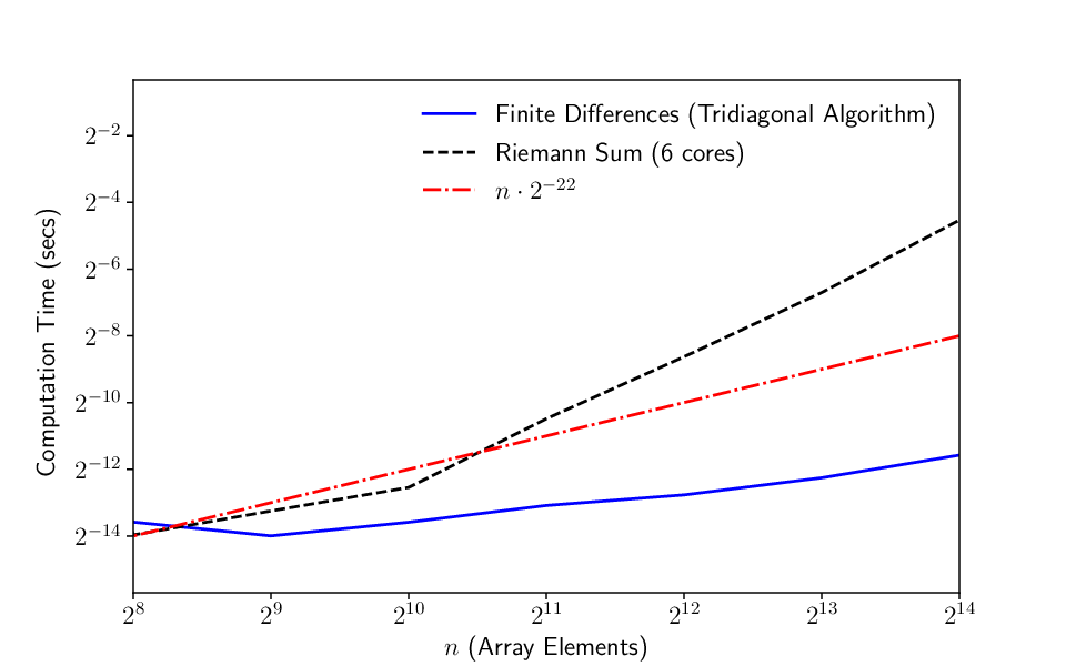
The matrix in (55) is tridiagonal, so banded matrix algorithms (Golub and Van Loan 2013) can be used to solve the corresponding system of equations. As shown in Fig. 2, using finite differences is much faster than a convolution (Riemann) sum, even when the embarrassing parallelism of the sum is exploited.
4.3.3 Particle Solver.
We solve the system of particle equations using the velocity Verlet algorithm (Mao et al. 2018). Given a system of ODEs of the form
| (57) |
with appropriate initial conditions and a time-discretization at steps with increment , the discretization is
| (58) |
5 Numerical Results and Higher Dimensions
In this section we present numerical simulations of one-dimensional nonlocal flocking dynamics, by solving the agent-based Cucker-Smale model using the velocity Verlet method, and the macroscopic model with initial conditions whose support is the interval . Our aim is to verify that the agent based and continuum based approaches to the flocking problem produce similar results.
In the following, the initial density and velocity are given by
| (59) | ||||
| (60) |
i.e. it is assumed that , where we have used .
5.1 Cucker-Smale Model Simulation
In all simulations, we take , . For the particle simulation, we use particles. For the macro-scale simulation, we use as the spatial increment. In both simulations, we take as the time increment.
In both cases, the support of the initial profile shrinks as the bulk comes together. The semi-linear Poisson-forced Euler system is highly dissipative, and the momentum profile is damped until it flattens (although it is conserved over the domain), and the system attains an equilibrium distribution. Fig. 3 shows the agreement between the particle model and the macro-scale model.

5.2 Higher Dimensions
In higher dimensions, the radial symmetry of the interaction function suggests the use of a singular kernel. Singular kernels have been extensively studied in the literature and, under mild assumptions in the initial conditions, have been shown to result in flocking behavior while, at the same time, avoiding collisions (Ahn et al. 2012).
In the BVP of the augmented system of PDEs (21) with the initial and boundary conditions (26), we select the linear differential operator (see also (Mavridis et al. 2020)):
| (61) |
and , which results in a Green’s function of the form
| (62) |
where is given by
| (63) | ||||
with being the modified Bessel function of the second kind of order , and is a function such that
| (64) | ||||
For we have
| (65) | ||||
and it can be shown that
| (66) |
The interaction function is affected by the bounded domain in the same way as in the one-dimensional case, and depends on the parameter values and as illustrated in Fig.4 for the -dimensional case.


6 Conclusion
A family of compactly supported parametric interaction functions in the general Cucker-Smale flocking dynamics was proposed such that the macroscopic system of mass and momentum balance equations with non-local damping terms can be converted to an augmented system of coupled PDEs in a compact set. We approached the computation of the non-local damping using the standard finite difference treatment of the chosen differential operator, which was solved using banded matrix algorithms. The expressiveness of the proposed interaction functions may be utilized for parametric learning from trajectory data.
References
- Ahn et al. (2012) Ahn, S., Choi, H., Ha, S.Y., and Lee, H. (2012). On collision-avoiding initial configurations to cucker-smale type flocking models. Communications in Mathematical Sciences, 10. 10.4310/CMS.2012.v10.n2.a10.
- Ballerini et al. (2008) Ballerini, M., Cabibbo, N., Candelier, R., Cavagna, A., Cisbani, E., Giardina, I., Lecomte, V., Orlandi, A., Parisi, G., Procaccini, A., et al. (2008). Interaction ruling animal collective behavior depends on topological rather than metric distance: Evidence from a field study. Proceedings of the national academy of sciences, 105(4), 1232–1237.
- Carrillo et al. (2010) Carrillo, J.A., Fornasier, M., Toscani, G., and Vecil, F. (2010). Particle, kinetic, and hydrodynamic models of swarming. In Mathematical modeling of collective behavior in socio-economic and life sciences, 297–336. Springer.
- Cucker and Smale (2007) Cucker, F. and Smale, S. (2007). Emergent behavior in flocks. IEEE Transactions on automatic control, 52(5), 852–862.
- Giardina (2008) Giardina, I. (2008). Collective behavior in animal groups: theoretical models and empirical studies. HFSP journal.
- Golub and Van Loan (2013) Golub, G.H. and Van Loan, C.F. (2013). Matrix Computations. The Johns Hopkins University Press, fourth edition.
- Ha et al. (2009) Ha, S.Y., Liu, J.G., et al. (2009). A simple proof of the cucker-smale flocking dynamics and mean-field limit. Communications in Mathematical Sciences, 7(2), 297–325.
- Kurganov and Tadmor (2000) Kurganov, A. and Tadmor, E. (2000). New high-resolution central schemes for nonlinear conservation laws and convection–diffusion equations. Journal of Computational Physics, 160(1), 241 – 282.
- LeVeque (2002) LeVeque, R.J. (2002). Finite Volume Methods for Hyperbolic Problems. Cambridge Texts in Applied Mathematics. Cambridge University Press. 10.1017/CBO9780511791253.
- Mao et al. (2018) Mao, Z., Li, Z., and Karniadakis, G. (2018). Nonlocal flocking dynamics: Learning the fractional order of pdes from particle simulations. arXiv preprint arXiv:1810.11596.
- Matei et al. (2019) Matei, I., Mavridis, C., Baras, J.S., and Zhenirovskyy, M. (2019). Inferring particle interaction physical models and their dynamical properties. In 2019 IEEE Conference on Decision and Control (CDC), 4615–4621. IEEE.
- Mavridis et al. (2020) Mavridis, C.N., Tirumalai, A., and Baras, J.S. (2020). Learning interaction dynamics from particle trajectories and density evolution. In 2020 59th IEEE Conference on Decision and Control (CDC). IEEE.
- Okubo (1986) Okubo, A. (1986). Dynamical aspects of animal grouping: swarms, schools, flocks, and herds. Advances in biophysics.
- Shvydkoy and Tadmor (2017) Shvydkoy, R. and Tadmor, E. (2017). Eulerian dynamics with a commutator forcing ii: Flocking. arXiv.
- Taylor (2010) Taylor, M. (2010). Partial Differential Equations I: Basic Theory. Applied Mathematical Sciences. Springer New York.