Rate-Splitting Multiple Access for Multi-Antenna Broadcast Channel with Imperfect CSIT and CSIR
PubID: pubid: 978-1-7281-4490-0/20/$31.00 © 2020 IEEE

Standard letter indicates scalar, lower case boldface letter denotes vector, and upper case boldface letter denotes matrix. Notation $\mathbf{A}\succeq\mathbf{B}$ indicates that matrix $\mathbf{A}-\mathbf{B}$ is positive semidefinite matrix. Superscript $(\cdot)^{H}$ denotes hermitian (conjugate transpose). Trace of matrix $\mathbf{A}$ is denoted by $\mathrm{tr}(\mathbf{A})$ and rank of matrix $\mathbf{A}$ is denoted by $\mathrm{rank}(\mathbf{A})$. Notations of $|\cdot|$, $||\cdot||$, and $\mathbb{E}[\cdot]$ refer to the absolute value, Euclidean norm, and expectation operation, respectively. A matrix $\mathbf{I}_{n}$ denotes a $n$ by $n$ identity matrix.

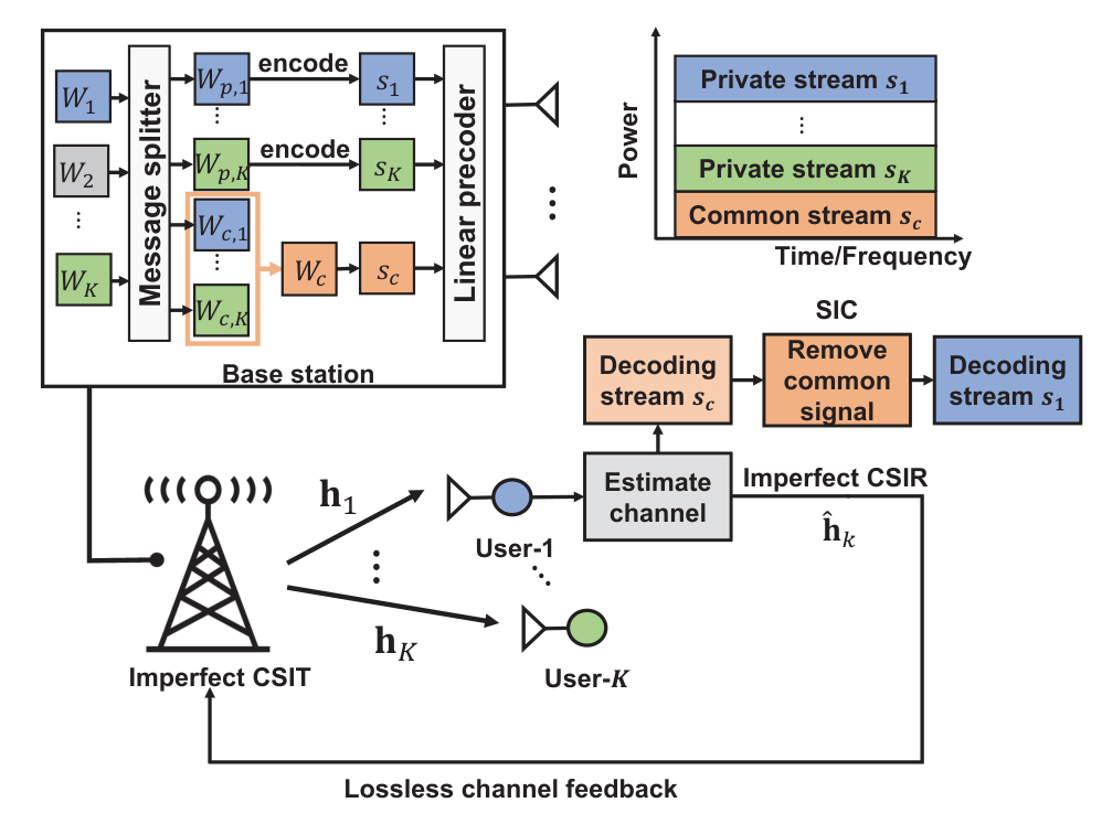
We consider a single cell MU-MISO system operating in downlink where the BS equipped with $N_{t}$ antennas serves $K$ single antenna users. As shown in Fig. 1, the main idea of RSMA is to split a message for user-$k$ $W_{k}$, $k=1,\dots,K$ into common and private parts, i.e. $W_{k}=\{W_{p,k},W_{c,k}\}$. The common part can be decoded by all users and the private part can be decoded by only the corresponding user. All common parts of each user message are combined into one common message $W_{c}$, i.e. $W_{c}=\{W_{c,1},\dots,W_{c,K}\}$. The common message $W_{c}$ is encoded into the common stream $s_{c}$ by using a codebook known to all users and each private message $W_{p,k}$ is encoded into the private stream $s_{k}$ by using a codebook known to only the intended receiver. Each stream is assumed to be independent zero mean unit variance Gaussian random variable, i.e. $s_{i}\sim\mathcal{CN}(0,1),~i\in\mathcal{I}\mathrel{\hbox{\hskip 3.8889pt\hskip-3.8889pt\hbox{$=$}\hskip-3.8889pt\hskip-2.7431pt\raisebox{4.66875pt}{\hbox{$\scriptscriptstyle\Delta$}}\hskip-2.7431pt\hskip 3.8889pt}}\{c,1,\dots,K\}.$ These $K+1$ streams are linearly precoded by using precoding vector $\mathbf{p}_{i}\in\mathbb{C}^{N_{t}\times 1},~i\in\mathcal{I}$. The transmitted signal at the BS is expressed as

where a transmitted signal power constraint with a total power $P_{t}$ is

We refer to $\mathbf{h}_{k}\in\mathbb{C}^{N_{t}\times 1}$ as a downlink channel vector from the BS to user-$k$ and a received signal at user-$k$ is denoted by

where $n\sim\mathcal{CN}(0,\sigma_{{n}}^{2})$ is additive white Gaussian noise (AWGN). Since the common stream can be decoded by all users, users can remove the common stream by SIC. Thus, users decode the private stream after SIC. When decoding the common stream, all private streams are treated as interference. When decoding a private stream, only other private streams are treated as interference, provided that the common stream is completely removed. Each user reconstructs the original message after retrieving the part of its message encoded in the common stream and the part encoded in the private stream.

We assume that users cannot accurately estimate the channel vector, i.e. imperfect CSIR. The channel model is given by

where $\hat{\mathbf{h}}_{k}$ is an estimated channel and $\mathbf{e}_{k}\sim\mathcal{CN}(0,\mathbf{\Phi}_{k})$ is a channel error. Also, we assume that the BS has the same CSI with the users because of lossless channel feedback. Thus, all users and the BS know the expectation of the channel, $\mathbb{E}[\mathbf{h}_{k}]=\hat{\mathbf{h}}_{k}$, and the covariance of the channel, $\mathbb{E}[(\mathbf{h}_{k}-\mathbb{E}[\mathbf{h}_{k}])(\mathbf{h}_{k}-\mathbb{E}[\mathbf{h}_{k}])^{H}]=\mathbf{\Phi}_{k}$. In this paper, it is assumed that the covariance matrix of channel error $\mathbf{e}_{k}$ is $\mathbf{\Phi}_{k}=\sigma_{\mathrm{e},k}^{2}\mathbf{I}$. In other words, the channel error is assumed as a vector of independent and identically distributed (i.i.d) random variables.

It is difficult to determine an explicit achievable rate under the imperfect CSIR assumption, since the users do not know the actual channel. Thus, the concept of generalized mutual information (GMI) is used in order to characterize the achievable rate at a user with imperfect CSI [8],[9]. We first introduce a general form of GMI by considering a point to point case for simplicity. When the input has Gaussian distribution $x\sim\mathcal{CN}(0,\epsilon_{x})$, the output signal is expressed by

where $h$ is the fading channel and $n\sim\mathcal{CN}(0,N)$ is the noise. When knowing expectation and variance of channel, $h$ can be broken into $\hat{h}$ and $e$, i.e. ${h}=\hat{h}+e$ where $\mathbb{E}[h]=\hat{h}$ and $\mathbb{E}[e]=0$. We can intuitively consider $\hat{h}$ as an estimate of the channel and $e$ as a channel error having zero mean with variance $\sigma_{h}^{2}$. GMI is defined by

where $\mathbb{E}[|e|^{2}]=\sigma^{2}_{h}$. In the case of imperfect CSIR, GMI corresponds to an achievable rate when a user uses a nearest neighbor decoder and the input is Gaussian distribution [10]. By using this property, we apply GMI to RSMA based system and derive the achievable rate under imperfect CSI.

In RSMA approach, a user first decodes the common stream and then decodes the corresponding private stream after SIC. By this feature, the rate of the private stream is derived using the received signal after SIC. The received signal at user-$k$ in (3) is rewritten as

Considering the common stream, the signal received from user-$k$ in (8) can be re-expressed in the form of (5) as

where ${h}_{k,c}=\hat{h}_{k,c}+e_{k,c}$, $\hat{h}_{k,c}=\hat{\mathbf{h}}_{k}^{H}\mathbf{p}_{\mathrm{c}}$, $e_{k,c}=\mathbf{e}_{k}^{H}\mathbf{p}_{\mathrm{c}}$, and $z_{\mathrm{c}}=\sum_{j=1}^{K}(\hat{\mathbf{h}}_{k}^{H}\mathbf{p}_{j}s_{j}+\mathbf{e}_{k}^{H}\mathbf{p}_{j}s_{j})+n$. Due to the independence between each stream and the noise, the expectation and variance of each component are derived as follows:

Substituting the values in (11), (13) and (14) into (6), the GMI for the common stream under imperfect CSIT can be obtained as

where $\mathbb{E}[|\mathbf{e}^{H}_{k}\mathbf{p}_{j}|^{2}]={\mathbf{p}_{j}^{\mathrm{H}}\mathbf{\Phi}_{k}\mathbf{p}_{j}}$, due to $\mathbb{E}[\mathbf{e}_{k}{\mathbf{e}_{k}}^{H}]=\mathbf{\Phi}_{k}$. Note that $|\mathbf{e}^{H}_{k}\mathbf{p}_{c}|^{2}$ is associated with not only the desired stream but also the channel error. Thus this term is considered as interference when decoding the desired stream, since users do not have any information on the channel error. The same phenomenon occurs when decoding the private streams.

When operating with perfect CSIR, the common stream can be removed perfectly by SIC. However, the common stream cannot be removed perfectly under imperfect CSIR, since the users do not have accurate information the actual channel. Thus, the part of the common stream associated with channel error still remains after SIC. The received signal after SIC with imperfect CSIR is expressed by

The rate of the private stream can be obtained in a similar manner as the common part. The received signal after SIC is rewritten as

where ${h}_{k}=\hat{h}_{k}+e_{k}$, $\hat{h}_{k}=\hat{\mathbf{h}}_{k}^{H}\mathbf{p}_{k}$, $e_{k}=\mathbf{e}_{k}^{H}\mathbf{p}_{k}$, and $z_{k}=\mathbf{e}_{k}^{H}\mathbf{p}_{c}s_{\mathrm{c}}+\sum_{\begin{subarray}{c}j=1\\ j\neq k\end{subarray}}^{K}(\hat{\mathbf{h}}_{k}^{H}\mathbf{p}_{j}s_{j}+\mathbf{e}_{k}^{H}\mathbf{p}_{j}s_{j})+n$. Thus, the achievable rate of private stream for user-$k$ with imperfect CSIR is determined as

Our objective is to optimize precoding vectors consisting of power and direction for maximizing the sum-rate. The sum-rate is expressed as

in which the common rate $R_{c}\mathrel{\hbox{\hskip 3.8889pt\hskip-3.8889pt\hbox{$=$}\hskip-3.8889pt\hskip-2.7431pt\raisebox{4.66875pt}{\hbox{$\scriptscriptstyle\Delta$}}\hskip-2.7431pt\hskip 3.8889pt}}\min_{k}R_{c,k},~k=1,\dots,K$ because the common stream is decoded by all users. The optimization problem for sum-rate maximization is formulated as:

We first simplify expression of the objective function of $\bm{\mathsf{(P1)}}$ using a stacking method introduced in [11]. First, we equivalently transform the expressions of the rate (15) and (20) as

and

By using a combined precoding vector $\mathbf{p}=[\mathbf{p}_{1}^{H},\dots,\mathbf{p}_{K}^{H},\mathbf{p}_{c}^{H}]^{H}\in\mathbb{C}^{N_{t}(K+1)\times 1}$, the numerator term in (23) can be expressed by

where $\mathbf{A}_{k}\in\mathbb{C}^{N_{t}(K+1)\times N_{t}(K+1)}$ is a block diagonal and positive definite matrix defined by

under the assumption that all transmission power is used, i.e., $\left\lVert\mathbf{p}\right\rVert^{2}=P_{t}$, and $\mathbf{\Phi}_{k}=\sigma_{\mathrm{e},k}^{2}\mathbf{I}$. We apply the same approach to the denominator and the numerator terms of (23), (24). Each term can be rewritten as:

where the positive definite matrix $\mathbf{B}_{k},\mathbf{D}_{k}$ are defined as

The matrix in the second term of (30) is a block diagonal matrix formulated by diag($\bm{0},\dots,\hat{\mathbf{h}}_{k}\hat{\mathbf{h}}{}^{H}_{k},\dots,\bm{0}$) in which $\hat{\mathbf{h}}_{k}\hat{\mathbf{h}}{}^{H}_{k}$ is a $k$th diagonal sub-block. As the result, the achievable rates are simplified to

and the objective function of the optimization problem $\bm{\mathsf{(P1)}}$ can also be simplified to

In this case, because $f(\mathbf{p})=f(\alpha\mathbf{p})$ with non-zero parameter $\alpha$, the power constraint (22b) can be ignored. Each rate is written as the difference of concave functions, e.g. $R_{k}=\log_{2}(\mathbf{p}^{H}\mathbf{B}_{k}\mathbf{p})-\log_{2}(\mathbf{p}^{H}\mathbf{D}_{k}\mathbf{p})$, which is a non-convex function. Thus, finding the optimal solution is difficult due to the non-convexity of the objective function. In order to solve the non-convex problem, we propose an algorithm based on alternating optimization.

Before finding a solution, to transform the problem, we derive upper and lower bounds of the denominator and numerator in (31) by using auxiliary variables $a_{k},b_{k},c_{k},d_{k}$:

Using these bounds, we can induce the lower bound of objective function $f(\mathbf{p})$ by

Finally, by adding one more slack variable $l_{c}$ for term of $\min_{j}(a_{j}-b_{j})$, the optimization problem $\bm{\mathsf{(P1)}}$ can be transformed to $\bm{\mathsf{(P2)}}$ denoted as

where $\mathbf{a}\mathrel{\hbox{\hskip 3.8889pt\hskip-3.8889pt\hbox{$=$}\hskip-3.8889pt\hskip-2.7431pt\raisebox{4.66875pt}{\hbox{$\scriptscriptstyle\Delta$}}\hskip-2.7431pt\hskip 3.8889pt}}[a_{1},\dots,a_{K}]$, $\mathbf{b}\mathrel{\hbox{\hskip 3.8889pt\hskip-3.8889pt\hbox{$=$}\hskip-3.8889pt\hskip-2.7431pt\raisebox{4.66875pt}{\hbox{$\scriptscriptstyle\Delta$}}\hskip-2.7431pt\hskip 3.8889pt}}[b_{1},\dots,b_{K}]$, $\mathbf{c}\mathrel{\hbox{\hskip 3.8889pt\hskip-3.8889pt\hbox{$=$}\hskip-3.8889pt\hskip-2.7431pt\raisebox{4.66875pt}{\hbox{$\scriptscriptstyle\Delta$}}\hskip-2.7431pt\hskip 3.8889pt}}[c_{1},\dots,c_{K}]$, and $\mathbf{d}\mathrel{\hbox{\hskip 3.8889pt\hskip-3.8889pt\hbox{$=$}\hskip-3.8889pt\hskip-2.7431pt\raisebox{4.66875pt}{\hbox{$\scriptscriptstyle\Delta$}}\hskip-2.7431pt\hskip 3.8889pt}}[d_{1},\dots,d_{K}]$. The problem is still non-convex, since the constraints (33), (34) are non-convex. For constraint (33), we apply SDR technique which obtains a solution that is close to the optimal solution in non-convex quadratically constrained quadratic program (QCQP) [12]. SDR converts a non-convex problem into a convex problem by removing the rank one constraint which causes non-convexity. To apply SDR, we transform the quadratic term of (33) as

by converting $\mathbf{p}\mathbf{p}^{H}$ to $\mathbf{X}$ with constraints $\mathbf{X}\succeq 0$ and $\mathrm{rank}(\mathbf{X})=1$. Then the constraint (33) becomes convex when the rank constraint is removed. Generally, an optimal solution of the relaxed problem may not satisfy the rank constraint, which implies that an additional process is required to construct a genuine solution that satisfies the rank constraint. This issue will be tackled after the algorithm is described.

The constraint functions in (34) are difference of convex (DC) functions that are generally non-convex. For this problem, we approximate the DC function to a convex function by the CCCP method, which guarantees a local optimal solution of the DC problem [13]. For such approximation, we linearize the exponential term in (34), which is concave, by using the first-order Taylor series approximation. Finally, constraints at the $s$th iteration can be denoted by

The sub-problem at $s$th iteration $\bm{\mathsf{(P3)}}$ is a convex problem expressed by

The value of $b_{k}^{(s-1)}$ and $d_{k}^{(s-1)}$ are updated by solving the sub-problem $\bm{\mathsf{(P3)}}$ and a local optimal solution is obtained with a sufficient number of iterations. The detailed process is expressed in Algorithm 1. The convex problem can be solved using CVX toolbox [14].

It is noted that a obtained solution $\mathbf{X}^{*}$ does not satisfy the constraint $\mathrm{rank}(\mathbf{X})=1$. Therefore, we refine $\mathbf{X}^{*}$ to satisfy the rank constraint. Since $\mathbf{X}^{*}$ is a Hermitian positive semidefinite matrix, it can be decomposed in the form $\mathbf{X}^{*}=\mathbf{U\Sigma U}^{H}$ by the singular value decomposition. Then, we generate sufficient number of random vectors $\mathbf{r}\in\mathbb{C}^{N_{t}(K+1)\times 1}$ and obtain $\mathbf{\bar{r}}=\mathbf{U\Sigma}^{1/2}\mathbf{r}$. Finally, we choose the best $\mathbf{\bar{r}}$ maximizing the objective function $f(\mathbf{p})$ as a final solution $\mathbf{p}^{*}$. It has been shown that SDR with sufficiently large number of random vectors guarantees a solution close to the optimal solution [12]. Overall step of the proposed algorithm is described in Algorithm 1.

$\mathbf{Remark~(Convergence):}$ In Algorithm 1, we randomly initialize the values of $b_{k}^{(0)}$ and $d_{k}^{(0)}$. In Fig. 2, it is numerically confirmed that the proposed algorithm converges to finite point as the number of iterations increases when SNR$=20$dB, $\sigma_{\mathrm{e},k}^{2}=0.1$. The value of objective function gradually increased without fluctuation. We can observe that as the number of transmitter antennas and users increases, the number of iterations required for convergence increases.

In this section, we consider a 2-user scenario and provide simulation results to compare with existing multiple access strategies: SDMA, NOMA, and OMA. It has been shown that these conventional strategies are special cases of RSMA in a 2-user scenario [5]. As shown in TABLE I, RSMA can boil down to conventional strategies depending on the power levels allocated to the streams. When user-1 has a stronger channel than user-2, the private stream of user-2 should be turned off, resulting in NOMA. Regardless of the number of users, RSMA works as SDMA when the common stream is turned off. Thus, the optimal power allocation and precoding vectors in NOMA and SDMA can be carried out by modifying Algorithm 1. Specifically, the precoding vector of the private stream of user-2 is set to zero vector in case of NOMA, while that of the common stream is set to zero vector in case of SDMA. Also, RSMA can be reduced to OMA by allocating the total transmit power to one private stream within a time slot. For OMA, we apply maximum ratio transmission (MRT) to precoding vector and assume that the same time resource is allocated to user-1 and user-2 for fairness.

In order to confirm the usefulness of the channel error information, a scenario in which the BS has no information about channel error, labeled as no-info $\sigma_{e}$, is further considered with the schemes described above. In other words, the BS optimizes the precoding vectors by considering $\hat{\mathbf{h}}_{k}$ as the perfect channel estimate. Note that in OMA, since the precoding vector and the power allocation are fixed, the sum-rate performance is not changed depending on whether or not there is no information about channel error in the BS.

We illustrate the achievable sum-rate of the proposed method according to SNR when the BS has two antennas and $\sigma_{\mathrm{e}}^{2}=0.05$. As shown in Fig. 3, RSMA has a better performance than other multiple accesses. The gap in sum-rate between RSMA and the other schemes is notable in high SNR. It is worth pointing out that these benefits come from the flexibility of RSMA that generalizes and bridges the conventional schemes for 2-user scenario. Compared to SDMA, the use of the common stream for RSMA, offers more design flexibility in jointly optimizing its precoding vector and power allocation. Under perfect CSIR, there is no increment of interference when a desired signal transmit power is increased. However, under imperfect CSIR, the interference from the channel error is also increased as the desired signal transmit power is increased. Thus, GMI and the sum-rate are saturated at high SNR. Furthermore, it is described in Fig. 3 that the performance is degraded in the absence of information about channel error and RSMA is less sensitive to the knowledge on channel errors than the other schemes.

In this section, performances of the precoding vectors are analyzed by comparing simulation results of RSMA with the proposed precoding vectors and existing fixed precoding vectors, zero-forcing (ZF) and MRT. ZF beamforming aims to remove the interference by nulling, i.e. $|\hat{\mathbf{h}}{}^{H}_{k}\mathbf{p}_{j}|=0,~j\neq k$ [15] and MRT refers to precoding the stream in the same direction with the channel vector. ZF and MRT are applied to the precoding vectors of the private streams. As shown in TABLE II, ZF and MRT determine the direction of the precoding vector for the private stream based on the estimated channel. As a result, the direction of the precoding vectors for the private stream, $\mathbf{v}_{k}=\mathbf{p}_{k}/\left\lVert\mathbf{p}_{k}\right\rVert,~k=1,\dots,K$, are fixed. Thus, power allocation, $P_{k}=\left\lVert\mathbf{p}_{k}\right\rVert$, and precoding vector for the common stream ${\mathbf{p}_{c}}$ should be optimized. We optimize the sum-rate of RSMA-ZF/MRT with the similar approach of the proposed RSMA by formulating an optimization problem for $P_{k}$ and ${\mathbf{p}_{c}}$.

Fig. 4 demonstrates the changes in the performance of RSMA with respect to channel error covariance $\sigma_{e}^{2}$ and SNR, where $K=2$ and $N_{t}=2$. The results confirm that the rate under imperfect CSI has different characteristics from that obtained under perfect CSI. Under perfect CSI, it is well known that MRT is near optimal in low SNR and ZF is asymptotically optimal in high SNR [16]. However, the imperfect knowledge of channel brings out the residual interference caused by the inaccurate operations of precoding (at the transmitter) as well as coherent detection including SIC (at the receiver), which corresponds to low SNR scenarios. When the variance of channel error, $\sigma_{e}^{2}$, is dominant, RSMA tends to operate as in low SNR under perfect CSI so that the optimized beamformers approximate to MRT. On the other hand, when channel error variance is very small, e.g. $\sigma_{e}^{2}\approx 0$, ZF can provide a better sum-rate perforamnce than that of MRT due to negligible residual interference at high SNR regime. As shown in Fig. 4, RSMA with the proposed precoding vector performs stricly better than RSMA with ZF and MRT precoders regardless of the variance of channel error over the entire range of SNR.

References

- [1] H. Joudeh and B. Clerckx, “Robust transmission in downlink multiuser MISO systems: A rate-splitting approach,” IEEE Transactions on Signal Processing, vol. 64, no. 23, pp. 6227-6242, Dec. 2016.
- [2] B. Clerckx, H. Joudeh, C. Hao, M. Dai, and B. Rassouli, “Rate splitting for MIMO wireless networks: A promising PHY-layer strategy for LTE evolution,” IEEE Communications Magazine, vol. 54, no. 5, pp. 98-105, May 2016.
- [3] Y. Mao, B. Clerckx, and V. O. K. Li, “Energy efficiency of rate-splitting multiple access, and performance benefits over SDMA and NOMA,” in Proc. 2018 15th International Symposium on Wireless Communication Systems (ISWCS), Lisbon, Portugal, Aug. 2018.
- [4] Y. Mao, B. Clerckx, and V.O.K. Li, “Rate-splitting multiple access for downlink communication systems: Bridging, generalizing and outperforming SDMA and NOMA,” EURASIP Journal on Wireless Communications and Networking, May 2018.
- [5] B. Clerckx, Y. Mao, R. Schober, and H. V. Poor, “Rate-splitting unifying SDMA, OMA, NOMA, and multicasting in MISO broadcast channel: A simple two-user rate analysis,” IEEE Wireless Communications Letters, vol. 9, no. 3, pp. 349-353, Mar. 2020.
- [6] Y. Mao, B. Clerckx, and V.O.K. Li, “Rate-splitting for multi-antenna non-orthogonal unicast and multicast transmission: Spectral and energy efficiency analysis,” IEEE Transactions on Communications, vol 67, no 12, pp. 8754-8770, Dec. 2019.
- [7] H. Joudeh and B. Clerckx, “Sum-rate maximization for linearly precoded downlink multiuser MISO systems with partial CSIT: A rate-splitting approach,” IEEE Transactions on Communications, vol. 64, no. 11, pp. 4847-4861, Nov. 2016.
- [8] Taesang Yoo and A. Goldsmith, “Capacity and power allocation for fading MIMO channels with channel estimation error,” IEEE Transactions on Information Theory, vol. 52, no. 5, pp. 2203-2214, May 2006.
- [9] M. Medard, “The effect upon channel capacity in wireless communications of perfect and imperfect knowledge of the channel,” IEEE Transactions on Information Theory, vol. 46, no. 3, pp. 933-946, May 2000.
- [10] A. Lapidoth and S. Shamai, “Fading channels: how perfect need ”perfect side information” be?,” IEEE Transactions on Information Theory, vol. 48, no. 5, pp. 1118-1134, May 2002.
- [11] J. Choi, N. Lee, S. Hong, and G. Caire, “Joint user selection, power allocation, and precoding design with imperfect CSIT for multi-cell MU-MIMO downlink systems,” IEEE Transactions on Wireless Communications, vol. 19, no. 1, pp. 162-176, Jan. 2020.
- [12] Z. Luo, W. Ma, A. M. So, Y. Ye, and S. Zhang, “Semidefinite relaxation of quadratic optimization problems,” IEEE Signal Processing Magazine, vol. 27, no. 3, pp. 20-34, May 2010.
- [13] Y. Sun, P. Babu, and D. P. Palomar, “Majorization-minimization algorithms in signal processing, communications, and machine learning,” IEEE Transactions on Signal Processing, vol. 65, no. 3, pp. 794-816, Feb. 2017.
- [14] M. Grant and S. Boyd, CVX: Matlab software for disciplined convex programming. (2013). [Online]. Available: http://cvxr.com/cvx/
- [15] A. Wiesel, Y. C. Eldar, and S. Shamai, “Zero-forcing precoding and generalized inverses,” IEEE Transactions on Signal Processing, vol. 56, no. 9, pp. 4409-4418, Sept. 2008.
- [16] E. Björnson, M. Bengtsson, and B. Ottersten, “Optimal multiuser transmit beamforming: A difficult problem with a simple solution structure [lecture notes],” IEEE Signal Processing Magazine, vol. 31, no. 4, pp. 142-148, July 2014.