跳到论文正文
W Papers独立论文阅读器 arXiv:2102.08573 论文正文 计算阅读时间 · 0%
引用这篇论文根据当前论文元数据生成,正式投稿前建议核对。


License: arXiv.org perpetual non-exclusive license
arXiv:2102.08573v5 [stat.AP] 07 Dec 2022

Robust Mean Estimation in High Dimensions: An Outlier-Fraction Agnostic and Efficient Algorithm

Aditya Deshmukh*, Student Member, IEEE, Jing Liu*, Member, IEEE, Venugopal V. Veeravalli, Fellow, IEEE Thanks: *Equal contribution. Thanks: A. Deshmukh and V.V. Veeravalli are with the ECE Department and Coordinated Science Lab, University of Illinois at Urbana-Champaign, Illinois, USA. Email: ad11,vvv@illinois.edu Thanks: J. Liu is with the Mitsubishi Electric Research Laboratories, Massachusetts, USA. Email: jiliu@merl.com Thanks: This research was supported by the US Army Research Laboratory under Cooperative Agreement W911NF-17-2-0196 and by the US National Science Foundation under grant 2106727, through the University of Illinois at Urbana-Champaign.
Abstract

The problem of robust mean estimation in high dimensions is studied, in which a certain fraction (less than half) of the datapoints can be arbitrarily corrupted. Motivated by compressive sensing, the robust mean estimation problem is formulated as the minimization of the ℓ0\ell_{0}-‘norm’ of an outlier indicator vector, under a second moment constraint on the datapoints. The ℓ0\ell_{0}-‘norm’ is then relaxed to the ℓp\ell_{p}-norm (0<p≤10<p\leq 1) in the objective, and it is shown that the global minima for each of these objectives are order-optimal and have optimal breakdown point for the robust mean estimation problem. Furthermore, a computationally tractable iterative ℓp\ell_{p}-minimization and hard thresholding algorithm is proposed that outputs an order-optimal robust estimate of the population mean. The proposed algorithm (with breakdown point ≈0.3\approx 0.3) does not require prior knowledge of the fraction of outliers, in contrast with most existing algorithms, and for p=1p=1 it has near-linear time complexity. Both synthetic and real data experiments demonstrate that the proposed algorithm outperforms state-of-the-art robust mean estimation methods.

Index Terms: 
Robust estimation, High-dimensional statistics, Global outlier pursuit, Linear time complexity algorithm

I Introduction

Robust mean estimation in high dimensions has received considerable interest recently, and has found applications in areas such as data analysis (e.g., spectral data in astronomy [1]), outlier detection [2, 3, 4] and distributed machine learning [5, 6, 7]. Classical robust mean estimation methods such as coordinate-wise median and geometric median have error bounds that scale with the dimension of the data [8], which results in poor performance in the high dimensional regime. A notable exception is Tukey’s Median [9] that has an error bound that is independent of the dimension, when the fraction of outliers is less than a threshold  [10, 11]. However, the computational complexity of Tukey’s Median algorithm is exponential in the dimension.

A number of recent papers have proposed polynomial-time algorithms that have dimension independent error bounds under certain distributional assumptions (e.g., bounded covariance or concentration properties). For a recent comprehensive survey on robust mean estimation, we refer the interested readers to [12]. One of the first such algorithms is Iterative Filtering [13, 14, 15], in which one finds the top eigenvector of the sample covariance matrix and removes (or down-weights) the points with large projection scores on that eigenvector, and then repeat this procedure on the rest of points until the top eigenvalue is small. However, as discussed in [4], the drawback of this approach is that it only looks at one direction/eigenvector at a time, and the outliers may not exhibit unusual bias in only one direction or lie in a single cluster. Figure 1 illustrates an example for which Iterative Filtering might have poor empirical performance. In this figure, the inlier datapoints in blue are randomly generated from the standard Gaussian distribution in (high) dimension dd, and therefore their ℓ2\ell_{2}-distances to the origin are roughly d\sqrt{d} (see, e.g., Theorem 3.1 of [16]). There are two clusters of outliers in red, and their ℓ2\ell_{2}-distances to the origin are also roughly d\sqrt{d}. If there is only one cluster of outliers, Iterative Filtering can effectively identify them; however, in this example, this method may remove many inlier points and perform suboptimally.

Refer to caption
Fig. 1: Illustration of two clusters of outliers (red points). The inlier points (blue) are drawn from standard Gaussian distribution in high dimension dd. Both the outliers and inliers are at roughly d\sqrt{d} distance from the origin.

There are interesting connections between existing methods for robust mean estimation and those used in compressive sensing. The Iterative Filtering algorithm has similarities to the greedy Matching Pursuit compressive sensing algorithm [17]. In the latter algorithm, one finds a single column of sensing matrix 𝑨\bm{A} that has largest correlation with the measurements 𝒃\bm{b}, removes that column and its contribution from 𝒃\bm{b}, and repeats this procedure on the remaining columns of 𝑨\bm{A}. Dong et al. [4] proposed a new scoring criteria for finding outliers, in which one looks at multiple directions associated with large eigenvalues of the sample covariance matrix in every iteration of the algorithm. Interestingly, this multi-directional approach is conceptually similar to Iterative Thresholding techniques in compressive sensing (e.g., Iterative Hard Thresholding [18] or Hard Thresholding Pursuit [19]), in which one simultaneously finds multiple columns of matrix 𝑨\bm{A} that are more likely contribute to 𝒃\bm{b}. Although iterative thresholding techniques are also greedy, they are more accurate than the Matching Pursuit technique in practice [20, 21].

A common assumption in robust mean estimation problem is that the fraction of the corrupted datapoints is small. In this paper, we explicitly use this information through the introduction of an outlier indicator vector whose ℓ0\ell_{0}-‘norm’ we minimize under a second moment constraint on the datapoints. This is partially motivated by compressive sensing and shares the same principle of ‘fitting the majority of the data’ that is common in robust statistics. This new formulation not only enables us to leverage advanced compressive sensing techniques to solve the robust mean estimation problem, but also allow us to design algorithms that do not require prior knowledge of the fraction of outliers. There are some works in sparse recovery (see, e.g. [22, 23]), in which ℓ0/ℓp\ell_{0}/\ell_{p} minimization is used to remove outliers in data. In these works, a linear model y=A​x+ey=Ax+e is considered, wherein yy denotes the measurements, the matrix AA is known, and the unknown sparse vector ee models the potential outlier corruption on each datapoint. Consequently, the analyses in the works on sparse recovery methods heavily rely on the assumption that the underlying model is linear (e.g., some works exploit the range-space/null-space properties of the matrix AA). On the other hand, in robust mean estimation, a general observation model (not necessarily linear) is considered. In light of this, the analyses in the works on sparse recovery cannot be transferred in an obvious way to the robust mean estimation problem.

We consider the setting in which the distribution of the datapoints before corruption has bounded covariance, as is commonly assumed in many recent works (e.g., [14, 4, 24, 25]). In particular, in  [24], the authors propose to minimize the spectral norm of the weighted sample covariance matrix and use the knowledge of the outlier-fraction ϵ\epsilon to constrain the weights. Along this line, two very recent works [26, 27] show that any approximate stationary point of the objective in [24] gives a near-optimal solution. In contrast, our objective is designed to minimize the sparsity of an outlier indicator vector, and we show that any sparse enough solution is nearly optimal.

Contributions:

  • •

    At a fundamental level, a contribution of this paper is the formulation of the robust mean estimation problem as minimizing the ℓ0\ell_{0}-‘norm’ of the proposed outlier indicator vector, under a second moment constraint on the datapoints. In addition, order-optimal estimation error guarantees and optimal breakdown point (ϵ<1/2)(\epsilon<1/2) are shown for this objective. We relax the ℓ0\ell_{0} objective to ℓp​(0<p≤1)\ell_{p}(0<p\leq 1) as in compressive sensing, and establish corresponding order-optimal estimation error guarantees. The guarantees are order-optimal with respect to the number of datapoints(nn), dimension of the data (dd), and the fraction of corrupted datapoints(ϵ\epsilon). Henceforth we use the term ‘order-optimal’ in this sense.

  • •

    Motivated by the proposed ℓ0\ell_{0} and ℓp\ell_{p} objectives and their theoretical justifications, we propose a computationally tractable iterative ℓp​(0<p≤1)\ell_{p}(0<p\leq 1) minimization and hard thresholding algorithm, and establish the order optimality of the algorithm. Empirical studies show that the proposed algorithm significantly outperforms state-of-the-art methods in robust mean estimation.

  • •

    The proposed algorithm (with maximal breakdown point of 1−1/21-1/\sqrt{2}) does not require the knowledge of the fraction of outliers (in contrast to most existing algorithms). For p=1p=1, the algorithm has near-linear time complexity.

II Proposed optimization problems

We begin by defining what we mean by a corrupted sample of datapoints.

Definition 1.

(ϵ\epsilon-corrupted sample [4]) Let PP be a distribution on ℝd\mathbb{R}^{d} with unknown mean 𝛍\bm{\mu}, and let 𝐲~1,…,𝐲~n\tilde{\bm{y}}_{1},...,\tilde{\bm{y}}_{n} be independent and identically distributed (i.i.d.) drawn from PP. These datapoints are then modified by an adversary who can inspect all the datapoints, remove ϵ​n\epsilon n of them, and replace them with arbitrary vectors in ℝd\mathbb{R}^{d}. We then obtain an ϵ\epsilon-corrupted sample, denoted as 𝐲1,…,𝐲n\bm{y}_{1},...,\bm{y}_{n}.

Throughout the rest of the paper, we adhere to the notation given above: we represent a datapoint before corruption as 𝒚~i\tilde{\bm{y}}_{i}, and after corruption as 𝒚i\bm{y}_{i}. Given a set of datapoints {𝒙i,i=1,…,n}\{\bm{x}_{i},i=1,\dots,n\}, we term the following as sample covariance matrix around 𝐳\bm{z}:

∑i=1n(𝒙i−𝒛)​(𝒙i−𝒛)⊤.\displaystyle\sum\limits_{i=1}^{n}(\bm{x}_{i}-\bm{z})(\bm{x}_{i}-\bm{z})^{\top}. (1)

There are other types of contamination one can consider, e.g., Huber’s ϵ\epsilon-contamination model [28]. The contamination model described in Definition 1 is the strongest in the sense that the adversary is not oblivious to the original datapoints, and can replace any subset of ϵ​n\epsilon n datapoints with any vectors in ℝd\mathbb{R}^{d}. We refer the reader to [12] for a more detailed discussion on contamination models.

Our primary goal is to robustly estimate the true population mean, given an ϵ\epsilon-corrupted sample. We assume that the underlying distribution has bounded second moment. A powerful and useful key insight that was exploited in previous work on the problem is that if the outliers in an ϵ\epsilon-corrupted sample (of large size) shift the average of datapoints before corruption by Ω⁡(ξ)\Omega(\xi) in a direction ν\nu, then the variance of the projected sample along ν\nu increases by Ω⁡(ξ2/ϵ)\Omega(\xi^{2}/\epsilon). Thus, intuitively, it suffices to find a large subset of the ϵ\epsilon-corrupted sample, whose sample covariance matrix is close to the covariance matrix of the underlying distribution. In order for such a subset to exist and for the mean of this large subset to be close to the true mean, we need some form of concentration of the datapoints (before corruption) around the mean of their distribution. A constrained second moment condition is sufficient to guarantee this, and such an assumption is also used in previous works. In the following, we provide a brief high-level explanation (details can be found in the Appendix). Suppose we are given a sufficiently large sample of datapoints of size nn, generated from a distribution with mean 𝝁\bm{\mu} and spectral norm of the covariance matrix bounded by σ2\sigma^{2}. Then, with high probability, there exists a large subset of the sample with spectral norm of the sample covariance matrix around 𝝁\bm{\mu} bounded by O⁡(σ2)O(\sigma^{2}). Hence, after corruption, with high probability there still exists a sufficiently large subset, say 𝑮∗\bm{G}^{*}, of the resulting ϵ\epsilon-corrupted sample, of size (1−ϵ′)​n(1-\epsilon^{\prime})n (where ϵ′→ϵ\epsilon^{\prime}\to\epsilon as n→∞n\to\infty), such that the spectral norm of the sample covariance matrix around 𝝁\bm{\mu} is bounded by O⁡(σ2)O(\sigma^{2}). Utilizing this, the concentration of the sample before corruption around 𝝁\bm{\mu}, and a fundamental result [27, Lemma C.2] about closeness of population mean and conditional mean, it can be shown that the distance between 𝝁\bm{\mu} and the sample average of 𝑮∗\bm{G}^{*} is O⁡(σ​ϵ′)O(\sigma\sqrt{\epsilon^{\prime}}).

Based on this motivation, we propose an ℓ0\ell_{0}-minimization problem to find the largest subset, whose sample covariance matrix exhibits bounded spectral norm. We first introduce an outlier indicator vector 𝒉\bm{h}: for the ii-th datapoint, hih_{i} indicates that whether it is an outlier (hi=1h_{i}=1) or not (hi=0h_{i}=0). Given an ϵ\epsilon-corrupted sample of size nn, we propose the following optimization problem, for which the solution in 𝒙\bm{x} should yield a robust estimate of the mean:

min𝒉,𝒙⁡‖𝒉‖0s.t.\displaystyle\min_{\bm{h},\bm{x}}\|\bm{h}\|_{0}\quad s.t.\ hi∈{0,1},∀i,\displaystyle h_{i}\in\{0,1\},\forall i, (2)
λmax​(∑i=1n(1−hi)​(𝒚i−𝒙)​(𝒚i−𝒙)⊤)≤c12​σ2​n,\displaystyle\lambda_{\mathrm{max}}\left(\sum_{i=1}^{n}(1-h_{i})(\bm{y}_{i}-\bm{x})(\bm{y}_{i}-\bm{x})^{\top}\right)\leq c_{1}^{2}\sigma^{2}n,

where c1c_{1} is a constant that controls the inflation of the constraint with respect to the bound (σ2)(\sigma^{2}) on the spectral norm of the covariance matrix of the underlying distribution.

We further relax the problem to the following:

min𝒉,𝒙⁡‖𝒉‖0s.t.\displaystyle\min_{\bm{h},\bm{x}}\|\bm{h}\|_{0}\quad s.t.\ 0≤hi≤1,∀i,\displaystyle 0\leq h_{i}\leq 1,\forall i, (3)
λmax​(∑i=1n(1−hi)​(𝒚i−𝒙)​(𝒚i−𝒙)⊤)≤c12​σ2​n.\displaystyle\lambda_{\mathrm{max}}\left(\sum_{i=1}^{n}(1-h_{i})(\bm{y}_{i}-\bm{x})(\bm{y}_{i}-\bm{x})^{\top}\right)\leq c_{1}^{2}\sigma^{2}n.

Note that any globally optimal solution of (2) is also globally optimal solution of (3). To see this, let 𝒉~\tilde{\bm{h}} be a global optimum of (3). Let 𝒉′\bm{h}^{\prime} be the vector obtained after setting the non-zero values of 𝒉~\tilde{\bm{h}} to 1. Note that 𝒉′\bm{h}^{\prime} has the same ℓ0\ell_{0}-norm as 𝒉~\tilde{\bm{h}}, and is also a feasible point of (2). Since the constraint set of (3) is larger than (2), the optimum value of (2) must be greater than or equal to the optimum value of (2). This implies that 𝒉′\bm{h}^{\prime} is a global optimum of (2). Hence, the claim holds. We show in Theorem 1, that any sparse enough feasible pair including the global optimum of (3) achieves order-optimality in terms of the error in estimating the mean.

However, minimizing the above ℓ0\ell_{0} objective is not computationally tractable. Motivated by compressive sensing, we further propose to relax the ℓ0\ell_{0}-‘norm’ to the ℓp\ell_{p}-norm (0<p≤10<p\leq 1), which leads to the following optimization problem:

min𝒉,𝒙⁡‖𝒉‖ps.t.\displaystyle\min_{\bm{h},\bm{x}}\|\bm{h}\|_{p}\quad s.t.\ 0≤hi≤1,∀i,\displaystyle 0\leq h_{i}\leq 1,\forall i, (4)
λmax​(∑i=1n(1−hi)​(𝒚i−𝒙)​(𝒚i−𝒙)⊤)≤c12​σ2​n.\displaystyle\lambda_{\mathrm{max}}\left(\sum_{i=1}^{n}(1-h_{i})(\bm{y}_{i}-\bm{x})(\bm{y}_{i}-\bm{x})^{\top}\right)\leq c_{1}^{2}\sigma^{2}n.

We show in Theorem 2, that even in this case any ‘good’ feasible pair including the global optimum is order-optimal in terms of the error in estimating the mean.

In the approaches taken in prior works (see, e.g., [27]), the robust mean estimation problem is the following feasibility problem:

Find ​h​ s.t. ​hi∈[0,1],∑i=1nhi≤ϵ​n,λmax​(∑i=1n(1−hi)​(yi−x)​(yi−x)⊤)≤C​σ2​n.\displaystyle\text{Find }h\text{ s.t. }h_{i}\in[0,1],\sum\limits_{i=1}^{n}h_{i}\leq\epsilon n,\lambda_{\max}(\sum\limits_{i=1}^{n}(1-h_{i})(y_{i}-x)(y_{i}-x)^{\top})\leq C\sigma^{2}n. (5)

Most works (see, e.g., [4, 24]) consider the following problem (or its variant), which is obtained by changing the feasibility problem into the following optimization problem:

min⁡λmax​(∑i=1n(1−hi)​(yi−x)​(yi−x)⊤)​ s.t. ​hi∈[0,1],∑i=1nhi≤ϵ​n\displaystyle\min\lambda_{\max}(\sum\limits_{i=1}^{n}(1-h_{i})(y_{i}-x)(y_{i}-x)^{\top})\text{ s.t. }h_{i}\in[0,1],\sum\limits_{i=1}^{n}h_{i}\leq\epsilon n (6)

where xx is either fixed or is the weighted average of yiy_{i}’s with weights as 1−hi1-h_{i}. Landscape results related to the optimization problem (6) were obtained in [24] and [27]. Our formulation (4), for the special case of p=1p=1, corresponds to minimizing the feasibility condition related to the sum of "weights" in (5). We provide landscape results for the optimization problem given in (4) (Theorems 1 and 2). An advantage of our formulation, which we will exploit in Algorithm 1, is that it does not require knowledge of the fraction of outliers ϵ\epsilon.

We now provide theoretical guarantees for the estimator which is given by the solution of the optimization problem (3). We show that given an ϵ\epsilon-corrupted sample of sufficiently large size, then with high probability, the ℓ2\ell_{2}-norm of the estimator’s error is O⁡(σ​ϵ+d​log⁡dn1−2​(ϵ+d​log⁡dn))O\left(\sigma\sqrt{\frac{\epsilon+\frac{d\log d}{n}}{1-2\left(\epsilon+\frac{d\log d}{n}\right)}}\right). We formalize this in the following theorem. It is well known that an information-theoretic lower bound on the ℓ2\ell_{2}-norm of any estimator’s error ‖𝒙^−𝝁‖2\|\hat{\bm{x}}-\bm{\mu}\|_{2} is Ω⁡(σ​ϵ1−2​ϵ)\Omega\left(\sigma\sqrt{\frac{\epsilon}{1-2\epsilon}}\right) (see [27]). Thus, the estimator is order-optimal in terms of the error as α→0\alpha\to 0 and n→∞n\to\infty.

Theorem 1.

Let PP be a distribution on ℝd\mathbb{R}^{d} with unknown mean 𝛍\bm{\mu} and unknown covariance matrix Σ⪯σ2​I\Sigma\preceq\ \sigma^{2}I. Let δ∈(0,1/4)\delta\in(0,1/4) and c1>1c_{1}>1 be fixed. Let c1′=c12​min⁡{c12​log⁡c12+1−c12,1}c_{1}^{\prime}=c^{2}_{1}\min\left\{c^{2}_{1}\log c^{2}_{1}+1-c^{2}_{1},1\right\}, n>2​ec1′​δ2​d​log⁡(d/δ)n>\frac{2e}{c_{1}^{\prime}\delta^{2}}d\log(d/\delta) and α=e​d​log⁡(d/δ)n​δ2​c1′\alpha=\frac{ed\log(d/\delta)}{n\delta^{2}c^{\prime}_{1}}. Let ϵ∈(0,1/2−α)\epsilon\in(0,1/2-\alpha) and ϵ′=ϵ+α\epsilon^{\prime}=\epsilon+\alpha. Given an ϵ\epsilon-fraction corrupted set of nn datapoints from PP, let

𝒮={(𝒉,𝒙):∥𝒉∥0<(1−ϵ′)n;𝒙=∑{i:hi=0}𝒚i|{i:hi=0}|}.\mathcal{S}=\left\{(\bm{h},\bm{x}):\|\bm{h}\|_{0}<(1-\epsilon^{\prime})n;{\bm{x}}=\frac{\sum_{\{i:{h}_{i}=0\}}\bm{y}_{i}}{|\{i:{h}_{i}=0\}|}\right\}. (7)

Then the following holds with probability at least 1−4​δ1-4\delta:
1) Any feasible pair (𝐡^,𝐱^)(\hat{\bm{h}},\hat{\bm{x}}) for the optimization problem (3) such that (𝐡^,𝐱^)∈𝒮(\hat{\bm{h}},\hat{\bm{x}})\in\mathcal{S} satisfies

‖𝒙^−𝝁‖2≤(c12​σ21−ϵ′+c12​σ21−‖𝒉^‖0n)​max⁡{ϵ′,‖𝒉^‖0n}1−ϵ′−‖𝒉^‖0n+c12​σ21−α.ϵ1−ϵ+σ​α​δ​(1+2​c1′e​log⁡(dδ)).\displaystyle\left\|\hat{\bm{x}}-\bm{\mu}\right\|_{2}\leq\left(\sqrt{\frac{c^{2}_{1}\sigma^{2}}{1-\epsilon^{\prime}}}+\sqrt{\frac{c^{2}_{1}\sigma^{2}}{1-\frac{\|\hat{\bm{h}}\|_{0}}{n}}}\right)\sqrt{\frac{\max\left\{\epsilon^{\prime},\frac{\|\hat{\bm{h}}\|_{0}}{n}\right\}}{1-\epsilon^{\prime}-\frac{\|\hat{\bm{h}}\|_{0}}{n}}}+\sqrt{\frac{c_{1}^{2}\sigma^{2}}{1-\alpha}.\frac{\epsilon}{1-\epsilon}}+{\sigma\sqrt{\alpha\delta}\left(1+2\sqrt{\frac{c_{1}^{\prime}}{e\log(\frac{d}{\delta})}}\right)}. (8)

2) A global optimum (𝐡opt,𝐱opt)(\bm{h}^{\mathrm{opt}},\bm{x}^{\mathrm{opt}}) of (3) lies in 𝒮\mathcal{S} with ‖𝐡opt‖0≤ϵ′​n\|\bm{h}^{\mathrm{opt}}\|_{0}\leq\epsilon^{\prime}n.

The proof is deferred to the Appendix. A high-level sketch of the proof of Theorems 1 is as follows. We use the idea in [27, Lemma 2.2] stated in Lemma 2. Informally, if two probability distributions on a set of datapoints are close in total variation distance, then the weighted means of the distributions are close. Consider the uniform distribution on the set {𝒚i:h^i=0}\{\bm{y}_{i}:\hat{h}_{i}=0\} (say P1P_{1}). Note that the estimator 𝒙^\hat{\bm{x}} in Theorem 1 is the mean of P1P_{1}. We show that the total variation distance between P1P_{1} and the uniform distribution (say P′P^{\prime}) on the set of inlier datapoints (that are within a distance of σ​dα​δ=σ​n​δ​c1′e​log⁡(d/δ)\sigma\sqrt{\frac{d}{\alpha\delta}}=\sigma\sqrt{\frac{n\delta c^{\prime}_{1}}{e\log(d/\delta)}} from 𝝁\bm{\mu}), is small. Therefore one can show that the distance between 𝒙^\hat{\bm{x}} and the mean of P′P^{\prime} is O⁡(σ​max⁡{ϵ′,‖𝒉^‖0n}1−ϵ′−‖𝒉^‖0n)O\left(\sigma\sqrt{\frac{\max\left\{\epsilon^{\prime},\frac{\|\hat{\bm{h}}\|_{0}}{n}\right\}}{1-\epsilon^{\prime}-\frac{\|\hat{\bm{h}}\|_{0}}{n}}}\right). Using Lemma 2, we show that the distance between the mean of P′P^{\prime} and 𝝁\bm{\mu} is O⁡(σ​ϵ′)O(\sigma\sqrt{\epsilon^{\prime}}). Using triangle inequality, it follows that the distance between 𝒙^\hat{\bm{x}} and 𝝁\bm{\mu} is O⁡(σ​max⁡{ϵ′,‖𝒉^‖0n}1−ϵ′−‖𝒉^‖0n)O\left(\sigma\sqrt{\frac{\max\left\{\epsilon^{\prime},\frac{\|\hat{\bm{h}}\|_{0}}{n}\right\}}{1-\epsilon^{\prime}-\frac{\|\hat{\bm{h}}\|_{0}}{n}}}\right).

Remark 1.

Theorem 1 shows that, as long as we find a feasible point 𝐡^\hat{\bm{h}} that is sparse enough, i.e., ‖𝐡^‖0≤(ϵ+α)​n\|\hat{\bm{h}}\|_{0}\leq(\epsilon+\alpha)n, the average of the estimated inliers ∑{i:h^i=0}𝐲i|{i:h^i=0}|\frac{\sum_{\{i:\hat{h}_{i}=0\}}\bm{y}_{i}}{|\{i:\hat{h}_{i}=0\}|} is close to the true mean in the optimal sense. It is not necessary to reach the global optimum of the objective (3).

We now provide a similar order-optimal error guarantee for the solution of the optimization problem in (4).

Theorem 2.

Let PP be a distribution on ℝd\mathbb{R}^{d} with unknown mean 𝛍\bm{\mu} and unknown covariance matrix Σ⪯σ2​I\Sigma\preceq\sigma^{2}I.Let δ∈(0,1/4)\delta\in(0,1/4), c1>1c_{1}>1 and p∈(0,1]p\in(0,1] be fixed. Let c1′=c12​min⁡{c12​log⁡c12+1−c12,1}c_{1}^{\prime}=c^{2}_{1}\min\left\{c^{2}_{1}\log c^{2}_{1}+1-c^{2}_{1},1\right\}, n>2​ec1′​δ2​d​log⁡(d/δ)n>\frac{2e}{c_{1}^{\prime}\delta^{2}}d\log(d/\delta) and α=e​d​log⁡(d/δ)n​δ2​c1′\alpha=\frac{ed\log(d/\delta)}{n\delta^{2}c^{\prime}_{1}}. Let ϵ∈(0,1/2−α)\epsilon\in(0,1/2-\alpha) and ϵ′=ϵ+α\epsilon^{\prime}=\epsilon+\alpha. Given an ϵ\epsilon-fraction corrupted set of nn datapoints from PP, let

𝒮′={(𝒉,𝒙):∥𝒉∥pp<(1−ϵ′)n;𝒙=∑i=1n(1−hi)​𝒚i∑i=1n(1−hi)}.\displaystyle\mathcal{S}^{\prime}=\left\{(\bm{h},\bm{x}):\|\bm{h}\|^{p}_{p}<(1-\epsilon^{\prime})n;\;\;{\bm{x}}=\frac{\sum_{i=1}^{n}(1-h_{i})\bm{y}_{i}}{\sum_{i=1}^{n}(1-h_{i})}\right\}. (9)

Then the following holds with probability at least 1−4​δ1-4\delta:

  1. 1.

    Any feasible pair (𝒉^,𝒙^)(\hat{\bm{h}},\hat{\bm{x}}) of (4) such that (𝒉^,𝒙^)∈𝒮′(\hat{\bm{h}},\hat{\bm{x}})\in\mathcal{S}^{\prime} satisfies

    ‖𝒙^−𝝁‖2≤(c12​σ21−ϵ′+c12​σ21−‖𝒉^‖ppn)​max⁡{ϵ′,‖𝒉^‖ppn}1−ϵ′−‖𝒉^‖ppn+c12​σ21−α.ϵ1−ϵ+σ​α​δ​(1+2​c1′e​log⁡(dδ)).\displaystyle\begin{split}\left\|\hat{\bm{x}}-\bm{\mu}\right\|_{2}\leq&\left(\sqrt{\frac{c^{2}_{1}\sigma^{2}}{1-\epsilon^{\prime}}}+\sqrt{\frac{c^{2}_{1}\sigma^{2}}{1-\frac{\|\hat{\bm{h}}\|^{p}_{p}}{n}}}\right)\sqrt{\frac{\max\left\{\epsilon^{\prime},\frac{\|\hat{\bm{h}}\|^{p}_{p}}{n}\right\}}{1-\epsilon^{\prime}-\frac{\|\hat{\bm{h}}\|^{p}_{p}}{n}}}+\sqrt{\frac{c_{1}^{2}\sigma^{2}}{1-\alpha}.\frac{\epsilon}{1-\epsilon}}\\ &+\sigma\sqrt{\alpha\delta}\left(1+2\sqrt{\frac{c_{1}^{\prime}}{e\log(\frac{d}{\delta})}}\right).\end{split} (10)
  2. 2.

    A global optimum (𝒉opt,𝒙opt)(\bm{h}^{\mathrm{opt}},\bm{x}^{\mathrm{opt}}) of (4) lies in 𝒮′\mathcal{S}^{\prime} with ‖𝒉opt‖pp≤ϵ′​n\|\bm{h}^{\mathrm{opt}}\|^{p}_{p}\leq\epsilon^{\prime}n.

The proof is deferred to the Appendix. The high-level idea is similar to that of the proof of Theorem 1. We consider the distribution on the α\alpha-corrupted samples with (normalized) probability weights 1−hi1-h_{i} (say P2P_{2}). Note that the estimator 𝒙^\hat{\bm{x}} in Theorem 2 is the mean of P2P_{2}. We show that the total variation distance between P2P_{2} and the uniform distribution (say P′P^{\prime}) on the set of inlier datapoints (that are within a distance of σ​dα​δ=σ​n​δ​c1′e​log⁡(d/δ)\sigma\sqrt{\frac{d}{\alpha\delta}}=\sigma\sqrt{\frac{n\delta c^{\prime}_{1}}{e\log(d/\delta)}} from 𝝁\bm{\mu}), is small. Therefore one can show that the distance between 𝒙^\hat{\bm{x}} and the mean of P′P^{\prime} is O⁡(σ​max⁡{ϵ′,‖𝒉^‖ppn}1−ϵ′−‖𝒉^‖ppn)O\left(\sigma\sqrt{\frac{\max\left\{\epsilon^{\prime},\frac{\|\hat{\bm{h}}\|^{p}_{p}}{n}\right\}}{1-\epsilon^{\prime}-\frac{\|\hat{\bm{h}}\|^{p}_{p}}{n}}}\right). Using Lemma 2, we show that the distance between the mean of P′P^{\prime} and 𝝁\bm{\mu} is O⁡(σ​ϵ′)O(\sigma\sqrt{\epsilon^{\prime}}). Using triangle inequality, it follows that the distance between 𝒙^\hat{\bm{x}} and 𝝁\bm{\mu} is O⁡(σ​max⁡{ϵ′,‖𝒉^‖ppn}1−ϵ′−‖𝒉^‖ppn)O\left(\sigma\sqrt{\frac{\max\left\{\epsilon^{\prime},\frac{\|\hat{\bm{h}}\|^{p}_{p}}{n}\right\}}{1-\epsilon^{\prime}-\frac{\|\hat{\bm{h}}\|^{p}_{p}}{n}}}\right).

Remark 2.

The breakdown point of the estimators in Theorems 1 and 2 is nearly the maximal possible 1/21/2 (as α→0\alpha\to 0 and n→∞n\to\infty), that is the estimator can tolerate any corruption level ϵ<1/2\epsilon<1/2, assuming that the number of samples nn satisfies the lower bound.

Remark 3.

From Lemma 6 in the Appendix, we know that given any feasible pair of (4) with ‖𝐡^‖p≤(ϵ′​n)1/p\|\hat{\bm{h}}\|_{p}\leq(\epsilon^{\prime}n)^{1/p}, we have that (𝐡^,∑i=1n(1−h^i)​𝐲i∑i=1n(1−h^i))\left(\hat{\bm{h}},\frac{\sum\limits_{i=1}^{n}(1-\hat{h}_{i})\bm{y}_{i}}{\sum\limits_{i=1}^{n}(1-\hat{h}_{i})}\right) is also a feasible pair, and therefore it lies in the set 𝒮′\mathcal{S}^{\prime} defined in (9). Theorem 2 further shows that this weighted average of the datapoints ∑i=1n(1−h^i)​𝐲i∑i=1n(1−h^i)\frac{\sum\limits_{i=1}^{n}(1-\hat{h}_{i})\bm{y}_{i}}{\sum\limits_{i=1}^{n}(1-\hat{h}_{i})} is close to the true mean. Again, we note that it is not necessary to reach the global optimum of the objective (4); we only need to find a feasible point 𝐡\bm{h} of (4) whose ℓp\ell_{p}-norm is small enough.

III Algorithm

III-A ℓp\ell_{p} minimization and thresholding

Motivated by the ℓp\ell_{p} objective and its theoretical guarantee, we propose an iterative ℓp\ell_{p} minimization algorithm. The algorithm, which is detailed in Algorithm 1, alternates between updating the outlier indicator vector 𝒉\bm{h} via minimizing its ℓp\ell_{p}-norm and updating the estimated mean 𝒙\bm{x}. To describe Algorithm 1, let ℋ\mathcal{H} be the set defined by

ℋ⁡(𝒙,c2)≔\displaystyle\mathcal{H}(\bm{x},c_{2})\coloneqq arg⁡min𝒉⁡‖𝒉‖p\displaystyle\arg\min_{\bm{h}}\|\bm{h}\|_{p} (11)
s.t.\displaystyle s.t.\quad 0≤hi≤1,∀i,\displaystyle 0\leq h_{i}\leq 1,\forall i,
λmax​(∑i=1n(1−hi)​(𝒚i−𝒙)​(𝒚i−𝒙)⊤)≤(c12+c22)​σ2​n.\displaystyle\lambda_{\mathrm{max}}\left(\sum_{i=1}^{n}(1-h_{i})(\bm{y}_{i}-\bm{x})(\bm{y}_{i}-\bm{x})^{\top}\right)\leq(c_{1}^{2}+c_{2}^{2})\sigma^{2}n.
Algorithm 1 Robust Mean Estimation via ℓp\ell_{p} Minimization and Thresholding
 Inputs:1) An ϵ\epsilon-corrupted set of datapoints {𝒚i}i=1n∈ℝd\{\bm{y}_{i}\}_{i=1}^{n}\in\mathbb{R}^{d} generated by a distribution whose covariance matrix satisfies Σ⪯σ2​I\Sigma\preceq\sigma^{2}I.2) Upper bound on corruption level: ϵˇ\check{\epsilon}3) Upper bound on spectral norm of Σ\Sigma: σ2\sigma^{2}.4) Threshold: 0<τ≤10<\tau\leq 1 such that f⁡(τ)>ϵˇf(\tau)>\check{\epsilon}, where f⁡(τ)f(\tau) is defined in (13), if such a τ\tau exists.5) Set c1>1c_{1}>1.6) Set 0<p≤10<p\leq 1 in ℓp\ell_{p}.
 Initialize:1) 𝒙(0)\bm{x}^{(0)} as the coordinate-wise median of {𝒚i}i=1n\{\bm{y}_{i}\}_{i=1}^{n}.2) c2(0)=3​d+2​c1c_{2}^{(0)}=3\sqrt{d}+2c_{1}.3) Iteration number t=0t=0.
 Do:
 Step 1: Given 𝒙(t)\bm{x}^{(t)}, update 𝒉\bm{h}:
 𝒉(t)∈ℋ⁡(𝒙(t),c2(t))\bm{h}^{(t)}\in\mathcal{H}(\bm{x}^{(t)},c_{2}^{(t)}), where ℋ\mathcal{H} is defined in (11).
 Step 2: Given 𝒉(t)\bm{h}^{(t)}, update 𝒙\bm{x}:𝒙(t+1)=∑i=1n(1−hi(t))1{hi(t)≤τ}𝒚i∑i=1n(1−hi(t))1{hi(t)≤τ}\bm{x}^{(t+1)}=\frac{\sum_{i=1}^{n}(1-h_{i}^{(t)})1\{h_{i}^{(t)}\leq\tau\}\bm{y}_{i}}{\sum_{i=1}^{n}(1-h_{i}^{(t)})1\{h_{i}^{(t)}\leq\tau\}}.c2(t+1)=γ⁡(ϵˇ)​c2(t)+β⁡(ϵˇ)c_{2}^{(t+1)}=\gamma(\check{\epsilon})c_{2}^{(t)}+\beta(\check{\epsilon}),where γ\gamma and β\beta are defined in (14) and (15)t=t+1t=t+1.
 While: t<T=1+log⁡c2(0)log⁡|γ⁡(ϵˇ)|t<T=1+\frac{\log c_{2}^{(0)}}{\log\lvert\gamma(\check{\epsilon})\rvert} and c2(t)<c2(t−1)c_{2}^{(t)}<c_{2}^{(t-1)}
 Output: 𝒙(T)\bm{x}^{(T)}

When updating the estimated mean 𝒙\bm{x} in Step 2 of Algorithm 1, we add an option to threshold the hih_{i} by τ\tau, so one can use the weighted average of the estimated ‘reliable’ datapoints (i.e., those for which hi≈0h_{i}\approx 0) to estimate 𝒙\bm{x}. This is motivated by the analysis of the original ℓ0\ell_{0} objective in Theorem 1, where the average of the estimated ‘reliable’ datapoints ∑{i:h^i=0}𝒚i|{i:h^i=0}|\frac{\sum_{\{i:\hat{h}_{i}=0\}}\bm{y}_{i}}{|\{i:\hat{h}_{i}=0\}|} is close to the true mean as long as the outlier indicator vector 𝒉^\hat{\bm{h}} is sparse enough. The breakdown point of Algorithm 1 depends on the threshold τ\tau and is given by f⁡(τ)f(\tau) (see (13)). The maximal breakdown point corresponds to no thresholding, i.e., f⁡(1)=1−1/2f(1)=1-1/\sqrt{2}. Algorithm 1 requires an upper bound ϵˇ\check{\epsilon} on the true fraction of outliers. This upper bound can be set arbitrarily close to (but less than) the breakdown point.

With this intuitive updating rule in Step 2, Algorithm 1 has following order-optimal guarantee.

Theorem 3.

Let PP be a distribution on ℝd\mathbb{R}^{d} with unknown mean 𝛍\bm{\mu} and unknown covariance matrix Σ⪯σ2​I\Sigma\preceq\sigma^{2}I. Let δ∈(0,1/5)\delta\in(0,1/5), c1>1c_{1}>1 and p∈(0,1]p\in(0,1] be fixed. Let τ∈(0,1]\tau\in(0,1], c1′=c12​min⁡{c12​log⁡c12+1−c12,1}c_{1}^{\prime}=c^{2}_{1}\min\left\{c^{2}_{1}\log c^{2}_{1}+1-c^{2}_{1},1\right\}, n>max⁡{90,ec1′​δ2​f​(τ)​d}​log⁡(d/δ)n>\max\left\{90,\frac{e}{c_{1}^{\prime}\delta^{2}f(\tau)}d\right\}\log(d/\delta), α=e​d​log⁡(d/δ)n​δ2​c1′\alpha=\frac{ed\log(d/\delta)}{n\delta^{2}c^{\prime}_{1}}. Let ϵ≥0\epsilon\geq 0 be such that 0<ϵ′≔ϵ+α≤ϵˇ<f⁡(τ)0<\epsilon^{\prime}\coloneqq\epsilon+\alpha\leq\check{\epsilon}<f(\tau). Given an ϵ\epsilon-fraction corrupted set of nn datapoints from PP, with probability at least 1−5​δ1-5\delta, all the iterates of Algorithm 1 (for t≥1t\geq 1) satisfy

‖𝒙(t)−𝝁‖2≤σ⁡[γ⁡(ϵ′)​(c2(0)​γ​(ϵˇ)t−1+1−γ​(ϵˇ)t−11−γ⁡(ϵˇ)​β​(ϵˇ))+β⁡(ϵ′)]+c1​σ​ϵ(1−α)​(1−ϵ)+σ​α​δ​(1+2​c1′e​log⁡(d/δ))\begin{split}\|{\bm{x}}^{(t)}-{{\bm{\mu}}}\|_{2}\leq\,&\sigma\left[\gamma(\epsilon^{\prime})\left(c_{2}^{(0)}\gamma(\check{\epsilon})^{t-1}+\frac{1-\gamma(\check{\epsilon})^{t-1}}{1-\gamma(\check{\epsilon})}\beta(\check{\epsilon})\right)+\beta(\epsilon^{\prime})\right]+c_{1}\sigma\sqrt{\frac{\epsilon}{(1-\alpha)(1-\epsilon)}}\\ &+{\sigma\sqrt{\alpha\delta}\left(1+2\sqrt{\frac{c_{1}^{\prime}}{e\log(d/\delta)}}\right)}\end{split} (12)

where c2(0)c_{2}^{(0)} is given in Algorithm 1, and

f⁡(τ)\displaystyle f(\tau) =3​τ+τ2−τ4+2​τ3+5​τ22​(1+τ)\displaystyle=\frac{3\tau+\tau^{2}-\sqrt{\tau^{4}+2\tau^{3}+5\tau^{2}}}{2(1+\tau)} (13)
γ⁡(ϵ)\displaystyle\gamma(\epsilon) =ϵ/τ(1−ϵ/τ)​(1−ϵ−ϵ/τ)\displaystyle=\sqrt{\frac{\epsilon/\tau}{(1-\epsilon/\tau)(1-\epsilon-\epsilon/\tau)}} (14)
β⁡(ϵ)\displaystyle\beta(\epsilon) =c1((1−ϵ/τ)−1/2+(1−ϵ)−1/2)ϵ/τ1−ϵ−ϵ/τ.\displaystyle=c_{1}\left((1-\epsilon/\tau)^{-1/2}+(1-\epsilon)^{-1/2}\right)\sqrt{\frac{\epsilon/\tau}{1-\epsilon-\epsilon/\tau}}. (15)

The output of Algorithm 1 at the end of T=1+log⁡c2(0)|log⁡γ⁡(ϵˇ)|=O⁡(log⁡d|log⁡ϵˇ|)T=1+\frac{\log c_{2}^{(0)}}{|\log\gamma(\check{\epsilon})|}=O\left(\frac{\log d}{|\log\check{\epsilon}|}\right) (when c2(0)≥β⁡(ϵˇ)1−γ⁡(ϵˇ)c_{2}^{(0)}\geq\frac{\beta(\check{\epsilon})}{1-\gamma(\check{\epsilon})}) or T=1T=1 (when c2(0)<β⁡(ϵˇ)1−γ⁡(ϵˇ)c_{2}^{(0)}<\frac{\beta(\check{\epsilon})}{1-\gamma(\check{\epsilon})}) iterations is order-optimal:

‖𝒙(T)−𝝁‖2≤σ⁡[γ⁡(ϵ′)​(1+β⁡(ϵˇ)1−γ⁡(ϵˇ))+β⁡(ϵ′)]+c1​σ​ϵ(1−α)​(1−ϵ)+σ​α​δ​(1+2​c1′e​log⁡(d/δ))=O⁡(σ​ϵ′).\begin{split}\|\bm{x}^{(T)}-\bm{\mu}\|_{2}&\leq\sigma\left[\gamma(\epsilon^{\prime})\left(1+\frac{\beta(\check{\epsilon})}{1-\gamma(\check{\epsilon})}\right)+\beta(\epsilon^{\prime})\right]+c_{1}\sigma\sqrt{\frac{\epsilon}{(1-\alpha)(1-\epsilon)}}+{\sigma\sqrt{\alpha\delta}\left(1+2\sqrt{\frac{c_{1}^{\prime}}{e\log(d/\delta)}}\right)}\\ &=O(\sigma\sqrt{\epsilon^{\prime}}).\end{split} (16)

The proof is deferred to the Appendix, but we briefly discuss the design of the algorithm and the high-level approach. Let 𝒙¯∗\bar{\bm{x}}^{*} be the average of the set of inlier datapoints that are within a distance of σ​dα​δ\sigma\sqrt{\frac{d}{\alpha\delta}} from 𝝁\bm{\mu}. We use induction to show that ‖𝒙(t)−𝒙¯∗‖≤c2(t)​σ\|\bm{x}^{(t)}-\bar{\bm{x}}^{*}\|\leq c_{2}^{(t)}\sigma. We show in the Appendix that the coordinate-wise median satisfies ‖𝒙(0)−𝝁‖2≤c2(0)​σ\|\bm{x}^{(0)}-\bm{\mu}\|_{2}\leq c_{2}^{(0)}\sigma with high probability. Firstly, observe that in Step 1 of Algorithm 1, the constraint on the spectral norm of the weighted covariance matrix around 𝒙(t)\bm{x}^{(t)} is (c12+(c2(t))2)​σ2​n\left(c_{1}^{2}+(c_{2}^{(t)})^{2}\right)\sigma^{2}n instead of c12​σ2​nc_{1}^{2}\sigma^{2}n as in (4). This ensures that with high probability that the optimization problem in Step 1 has a feasible point, and that the optimum solution satisfies ‖𝒉(t)‖p≤(ϵ′​n)1/p\|\bm{h}^{(t)}\|_{p}\leq(\epsilon^{\prime}n)^{1/p}. Secondly, we exploit the boundedness of ‖𝒉(t)‖p\|\bm{h}^{(t)}\|_{p} and the fact that the spectral norm of the weighted covariance matrix around 𝒙(t)\bm{x}^{(t)} is bounded (similar to the idea used in Theorem 2), along with some concentration bounds to show that in each iteration the iterate 𝒙(t+1)\bm{x}^{(t+1)} in Step 2 moves closer to μ\mu than 𝒙(t)\bm{x}^{(t)}. Specifically, we show that ‖𝒙(t+1)−𝝁‖2≤γ​‖𝒙(t)−𝝁‖2+β​σ≤(γ​c2(t)+β)​σ=c2(t+1)​σ\|\bm{x}^{(t+1)}-\bm{\mu}\|_{2}\leq\gamma\|\bm{x}^{(t)}-\bm{\mu}\|_{2}+\beta\sigma\leq(\gamma c_{2}^{(t)}+\beta)\sigma=c_{2}^{(t+1)}\sigma, where γ<1\gamma<1. From the proof we can see that it is not necessary to reach the global optimum in Step 1, we only need to find a feasible point whose ℓp\ell_{p}-norm is small enough.

Remark 4.

The results of Theorems 1, 2 and 3 can be easily extended to establish the estimators’ closeness to the average of the datapoints before corruption, 𝛍~=1n​∑i=1n𝐲~i\tilde{\bm{\mu}}=\frac{1}{n}\sum\limits_{i=1}^{n}\tilde{\bm{y}}_{i}, using the fact that 𝛍~\tilde{\bm{\mu}} is close to 𝛍\bm{\mu}, which is shown in the Appendix ((see (32))). We obtain the following extension to the above theorems with the same probability guarantees:

‖𝒙^−𝝁~‖2≤‖𝒙^−𝝁‖2+σ​dn​δ.\displaystyle\|\hat{\bm{x}}-\tilde{\bm{\mu}}\|_{2}\leq\|\hat{\bm{x}}-\bm{\mu}\|_{2}+{\sigma\sqrt{\frac{d}{n\delta}}}. (17)

Moreover, it can be also shown that the estimators are close to the average of inliers, that are at most a distance of σ​dα​δ=σ​n​δ​c1′e​log⁡(d/δ)\sigma\sqrt{\frac{d}{\alpha\delta}}=\sigma\sqrt{\frac{n\delta c^{\prime}_{1}}{e\log(d/\delta)}} from 𝛍\bm{\mu}.

Remark 5.

The initialization c2(0)=3​d+2​c1c_{2}^{(0)}=3\sqrt{d}+2c_{1} can be replaced by a smaller value as long as it is possible to guarantee ‖𝐱(0)−𝛍‖2≤c2(0)​σ\|\bm{x}^{(0)}-\bm{\mu}\|_{2}\leq c_{2}^{(0)}\sigma with high probability.

An important aspect of the proposed algorithm is that it does not require the true fraction of outliers ϵ\epsilon and is still order-optimal. To the best of our knowledge no other algorithm for our corruption model has this property.

III-B Solving Step 1 of Algorithm 1

When we set p=1p=1 in the objective ‖𝒉‖p\|\bm{h}\|_{p} in Step 1 of Algorithm 1, the resulting problem is convex, and can be reformulated as the following packing SDP  [29] with wi≜1−hiw_{i}\triangleq 1-h_{i}, and eie_{i} being the ii-th standard basis vector in ℝn\mathbb{R}^{n}. The details can be found in the Appendix.

max𝒘⁡ 1⊤​𝒘s.t.\displaystyle\max_{\bm{w}}\ \bm{1}^{\top}\bm{w}\quad s.t. wi≥0,∀i\displaystyle\ w_{i}\geq 0,\forall i (18)
∑i=1nwi​[ei​ei⊤(𝒚i−𝒙)​(𝒚i−𝒙)⊤]⪯[In×nc​n​σ2​Id×d]\displaystyle\sum_{i=1}^{n}w_{i}\begin{bmatrix}e_{i}e_{i}^{\top}&\\ &(\bm{y}_{i}-\bm{x})(\bm{y}_{i}-\bm{x})^{\top}\end{bmatrix}\preceq\begin{bmatrix}I_{n\times n}&\\ &cn\sigma^{2}I_{d\times d}\end{bmatrix}

When 0<p<10<p<1, the equivalent objective function ‖𝒉‖pp=∑ihip\|\bm{h}\|_{p}^{p}=\sum_{i}h_{i}^{p} is concave, not convex. So it may be difficult to find its global minimum. Nevertheless, we can iteratively construct and minimize a tight upper bound on this objective function via iterative re-weighted ℓ2\ell_{2} [30, 31] or ℓ1\ell_{1} techniques [32] from compressive sensing.11 1 We observe that iterative re-weighted ℓ2\ell_{2} achieves better empirical performance. And it is well-known in compressive sensing that such iterative re-weighted approaches often performs better than ℓ1\ell_{1} [32, 30].

III-C Complexity analysis

Theorem 3 guarantees that the total number of iterations of Algorithm 1 required to achieve optimality is upper bounded by O⁡(log⁡dlog⁡|ϵˇ|)O(\frac{\log d}{\log\left\lvert\check{\epsilon}\right\rvert}). In each iteration, the computational complexity of Step 2 is O⁡(n​d)O(nd). It follows easily from the proof of Theorem 3, that it suffices to solve the SDP in step 1 of Algorithm 1 (with p=1p=1) to a constant precision. As a result, the error is affected by a constant and thus remains order-optimal and the time complexity is O~​(n​d)\tilde{O}(nd) parallelizable work using positive SDP solvers [33] (the notation O~​(m)\tilde{O}(m) hides the poly-log factors: O~(m)=O(m.polylog(m))\tilde{O}(m)=O(m.\text{polylog}(m))). A comparison of our theoretical results with those in state-of-the-art works is given in Table I.

If we use ℓp\ell_{p} with 0<p<10<p<1 in Step 1, we iteratively construct and minimize a tight upper bound on the ℓp\ell_{p} objective via iterative re-weighted ℓ2\ell_{2} [30, 31] or iterative re-weighted ℓ1\ell_{1} techniques [32]22 2 We run fewer than 10 re-weighted iterations in our implementation.. Minimizing the resulting weighted ℓ1\ell_{1} objective can be also solved very efficiently to a constant precision by formulating it as a Packing SDP (see Appendix) with computational complexity of O~​(n​d)\tilde{O}(nd) [33]. If we use iterative re-weighted ℓ2\ell_{2}, minimizing the resulting weighted ℓ2\ell_{2} objective is a SDP constrained least squares problem, whose computational complexity is in general polynomial in both dd and nn. We will explore more efficient solutions for this objective in future work.

Algorithm Time complexity Error guarantee Breakdown point Requires ϵ\epsilon
Tukey median [11] NP-hard O⁡(σ​ϵ)O(\sigma\sqrt{\epsilon}) 1d+1\frac{1}{d+1} No
IF [14] O~​(n​d2)\tilde{O}(nd^{2}) O⁡(σ​ϵ)O(\sigma\sqrt{\epsilon}) N​ANA Yes
GF [27] O~​(n2​d)\tilde{O}(n^{2}d) O⁡(σ​ϵ1−2​ϵ)O\left(\sigma\frac{\sqrt{\epsilon}}{1-2\epsilon}\right) 12\frac{1}{2} Yes
CDG [24] O~​(n​dϵ6)\tilde{O}\left(\frac{nd}{\epsilon^{6}}\right) O⁡(σ​ϵ)O(\sigma\sqrt{\epsilon}) 13\frac{1}{3} Yes
QUE [4] O~​(n​d)\tilde{O}(nd) O⁡(σ​ϵ)O(\sigma\sqrt{\epsilon}) NA Yes
Proposed optimization problems (ℓp,p∈[0,1])(\ell_{p},p\in[0,1]) NA O⁡(σ​ϵ1−2​ϵ)O\left(\sigma\sqrt{\frac{\epsilon}{1-2\epsilon}}\right) 12\frac{1}{2} No
Proposed algorithm (p=1)(p=1) O~​(n​d)\tilde{O}(nd) O⁡(σ​ϵ)O(\sigma\sqrt{\epsilon}) 1−12≈0.31-\frac{1}{\sqrt{2}}\approx 0.3 No
TABLE I: Theoretical comparison

IV Empirical Studies

In this section, we present empirical results on the performance of Algorithm 1 and compare with the following state-of-the-art high dimension robust mean estimation methods: Iterative Filtering (IF) [14], Generalized Filtering (GF) [27, Algorithm 2], the method proposed in [8] (denoted as LRV), the method for bounded covariance distributions in [24] (denoted as CDG), and Quantum Entropy Scoring (QUE) [4], which scores the outliers based on multiple directions. We briefly discuss the implementation details of these algorithms. We implemented the QUE method by utilizing the code provided in [4]. In [24], the authors provide a way to implement the CDG method approximately; we provide results for an exact implementation of the CDG method. Since the number of datapoints considered in the following simulations is less than the minimum requirement, a reasonable approach to compare the performance of the algorithms is to tune the hyper-parameters of all algorithms to get the best possible error. For example, the hyper-parameter c4c_{4} that appears in CDG method [24], is set to be 1.051.05, which produced the smallest empirical error. The value of σ\sigma provided to the algorithms is not the theoretical value, but the empirical one (precisely, the spectral norm of the sample covariance matrix of G∗G^{*} (see Section II)). For evaluation purposes, we report the recovery error, which we define it as the ℓ2\ell_{2} distance of the estimated mean to the oracle solution, i.e., the average of the uncorrupted datapoints after corruption.

IV-A Synthetic data

We consider two experimental settings. For the first setting we follow [4]. The dimension of the data is dd, and the number of datapoints is nn. The inlier datapoints are generated i.i.d. according to the standard Gaussian distribution with zero mean. Randomly (uniformly) chosen ϵ\epsilon fraction of the datapoints are replaced by outliers. For the outliers, half of them are set to be (d/2,d/2,0,…,0)⊤(\sqrt{d/2},\sqrt{d/2},0,...,0)^{\top}, and the other half are set as (d/2,−d/2,0,…,0)⊤(\sqrt{d/2},-\sqrt{d/2},0,...,0)^{\top}, so that their ℓ2\ell_{2} distances to the population mean (0,…,0)⊤(0,...,0)^{\top} are all d\sqrt{d}, similar to that of the inlier points. These are two clusters of outliers, and their ℓ2\ell_{2} distances to the true mean 𝒙\bm{x} are similar to that of the inlier points. In Algorithm 1, we set the threshold τ=0.6\tau=0.6, c1=1.1c_{1}=1.1, and we initialize c2(0)c_{2}^{(0)} as the ℓ2\ell_{2} error of the coordinate-wise Median relative to the true mean. We implemented the IF method for sub-Gaussian parameters [14, Theorem 3.1]. We vary the total fraction ϵ\epsilon of the outliers and report the average recovery error of each method over 10 trials in Table II with d=100,n=1000d=100,n=1000. The proposed ℓ1\ell_{1} and ℓ0.5\ell_{0.5} methods show significant improvements over the competing methods, and the ℓ0.5\ell_{0.5} method performs the best.

TABLE II: Recovery error of each method under different fraction ϵ\epsilon of the outlier points (d=100,n=1000d=100,n=1000)
ϵ\epsilon IF GF QUE LRV CDG ℓ1\ell_{1} ℓ0.5\ell_{0.5}
10% 0.124 0.098 0.429 0.367 0.064 0.013 0.006
20% 0.131 0.115 0.492 0.659 0.084 0.013 0.007

We also tested the performance of each method for different numbers of datapoints. The dimension of the data is fixed to be 100. The fraction of the corrupted points is fixed to be 20%. We vary the number of datapoints from 100 to 1000, and report the average recovery error for each method over 50 trials in Table III. We can see that the performance of all methods get better when the number of datapoints is increased. Again, our proposed methods consistently perform better than the other methods.

TABLE III: Recovery error of each method w.r.t. different number of samples (d=100,ϵ=0.2d=100,\epsilon=0.2)
nn IF GF QUE LRV CDG ℓ1\ell_{1} ℓ0.5\ell_{0.5}
100 0.493 0.293 1.547 1.423 0.316 0.060 0.033
200 0.313 0.239 1.038 1.084 0.198 0.036 0.021
500 0.186 0.170 0.680 0.794 0.148 0.021 0.012
1000 0.131 0.115 0.492 0.659 0.084 0.013 0.007

The second experimental setting is as follows. The dimension of the data is dd, and the number of datapoints is nn. The inlier datapoints are generated i.i.d. such that each coordinate follows the Pareto distribution with scale parameter as 11 and shape parameter as 2.52.5. This implies that each coordinate has bounded second moment but no higher moments. All outliers are set to be the same vector 𝒗\bm{v} which is chosen as follows. Let gg be the average of the ℓ2\ell_{2} norms of the datapoints. The vector 𝒗\bm{v} is set as (2+g/d,2+g/d,…,2+g/d)⊤(2+\sqrt{g/d},2+\sqrt{g/d},\dots,2+\sqrt{g/d})^{\top}. Randomly (uniformly) chosen ϵ\epsilon fraction of the datapoints are replaced by outliers. The LRV method is applicable only to cases where distributions have bounded fourth moment, and hence is not applicable to this setting. The CDG method was not implemented due to the high computational complexity of its implementation. We implemented the IF method for bounded second moment parameters  [14, Theorem 3.2]. We implemented Algorithm 1 with p=1p=1, τ=1\tau=1(no thresholding during the iterations), c1=1c_{1}=1 and c2(0)=3​d+2​c1c_{2}^{(0)}=3\sqrt{d}+2c_{1}. However, we threshold the last iterate h(T)h^{(T)} with threshold 0.60.6. We vary the total fraction ϵ\epsilon of the outliers and report the average recovery error of each method over 100 trials in Table IV with d=1000,n=100000d=1000,n=100000. The proposed ℓ1\ell_{1} method show significant improvement over the competing methods. We also tested the performance of each method for two different numbers of datapoints. The dimension of the data is fixed to be 1000. The fraction of the corrupted points is fixed to be 20%. We consider the number of datapoints to be 10000 and 100000, and report the average recovery error for each method over 100 trials in Table V. Again, the proposed method consistently perform better than the other methods.

TABLE IV: Recovery error of each method under different fraction ϵ\epsilon of the outlier points (d=1000,n=100000d=1000,n=100000)
ϵ\epsilon IF GF QUE ℓ1\ell_{1}
10% 0.0164 0.0550 0.1096 0.0161
20% 0.0845 0.0726 0.2489 0.0190
TABLE V: Recovery error of each method w.r.t. different number of samples (d=1000,ϵ=0.2d=1000,\epsilon=0.2)
nn IF GF QUE ℓ1\ell_{1}
10000 0.3027 0.0780 0.3991 0.0257
100000 0.0845 0.0726 0.2489 0.0190

IV-B Corrupted image dataset

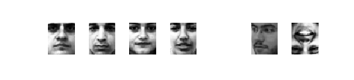
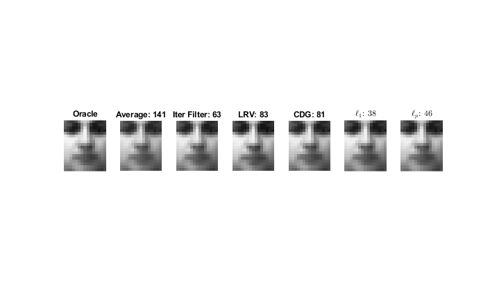
Here we use a dataset of real face images to test the effectiveness of the robust mean estimation methods. The average face of particular regions or certain groups of people is useful for many social and psychological studies [34]. Here we use 100 frontal human face images from the Brazilian face database33 3 https://fei.edu.br/ cet/facedatabase.html as inliers. For the outliers, we choose 15 face images of cats and dogs from the CIFAR10 [35] database. In order to be able to run the CDG method [24], we scale the size of images to 18 ×\times 15 pixels, so the dimension of each datapoint is 270. The oracle solution is the average of the 100 human faces. Table VI reports the recovery error, which is the ℓ2\ell_{2} distance of the estimated mean to the oracle solution, for each method. The proposed methods achieve smaller recovery error than the state-of-the-art methods. The sample inlier and outlier images as well as the estimated mean for each method can be found in the Appendix.

TABLE VI: Recovery error of the mean face by each method
Sample average IF LRV CDG ℓ1\ell_{1} ℓ0.5\ell_{0.5}
141 63 83 81 38 46

V Conclusion

We formulated the robust mean estimation problems as the minimization of the ℓ0\ell_{0}-‘norm’ of the introduced outlier indicator vector, under a second moment constraint on the datapoints. We further relaxed the ℓ0\ell_{0} objective to an ℓp\ell_{p} (0<p≤1)(0<p\leq 1) objective, and theoretically justified the new objective. The proposed ℓ0\ell_{0} and ℓp\ell_{p} optimization problems do not need to know ϵ\epsilon, and still achieve information-theoretically order-optimal error bounds with optimal breakdown points. Then we proposed a computationally tractable iterative ℓp​(0<p≤1)\ell_{p}(0<p\leq 1) minimization and hard thresholding algorithm, which significantly outperforms state-of-the-art robust mean estimation methods, and is order-optimal. In the empirical studies, we observed strong numerical evidence that using the ℓp\ell_{p} (0<p≤1)(0<p\leq 1) norm in the optimization leads to sparse solutions; theoretically justifying this phenomenon is also of interest. It is worth noting that almost all previous polynomial-time methods (with dimension-independent error bound) need to know ϵ\epsilon, while our Algorithm 1 does not require to know ϵ\epsilon. It has a maximal breakdown point of 1−1/21-1/\sqrt{2}, and has near-linear time complexity for p=1p=1.

References

  • [1] R. A. Maronna and R. H. Zamar, “Robust estimates of location and dispersion for high-dimensional datasets,” Technometrics, vol. 44, no. 4, pp. 307–317, 2002.
  • [2] P. J. Huber, Robust statistics. New York: Wiley, 2004.
  • [3] R. A. Maronna, R. D. Martin, V. J. Yohai, and M. Salibián-Barrera, Robust statistics: theory and methods (with R). New York: Wiley, 2019.
  • [4] Y. Dong, S. Hopkins, and J. Li, “Quantum entropy scoring for fast robust mean estimation and improved outlier detection,” in Advances in Neural Information Processing Systems 32. Curran Associates, Inc., 2019, pp. 6067–6077.
  • [5] Y. Chen, L. Su, and J. Xu, “Distributed statistical machine learning in adversarial settings: Byzantine gradient descent,” in Proc. ACM Measurement and Analysis of Computing Systems, vol. 1, no. 2. ACM New York, NY, USA, 2017, pp. 1–25.
  • [6] D. Yin, Y. Chen, R. Kannan, and P. Bartlett, “Byzantine-robust distributed learning: Towards optimal statistical rates,” in International Conference on Machine Learning, 2018, pp. 5650–5659.
  • [7] S. Bubeck, N. Cesa-Bianchi, and G. Lugosi, “Bandits with heavy tail,” IEEE Transactions on Information Theory, vol. 59, no. 11, pp. 7711–7717, 2013.
  • [8] K. A. Lai, A. B. Rao, and S. Vempala, “Agnostic estimation of mean and covariance,” in 2016 IEEE 57th Annual Symposium on Foundations of Computer Science (FOCS), 2016, pp. 665–674.
  • [9] J. W. Tukey, “Mathematics and the picturing of data,” in Proceedings of the International Congress of Mathematicians, vol. 2, Vancouver, August 1975, pp. 523–531.
  • [10] D. L. Donoho, M. Gasko et al., “Breakdown properties of location estimates based on halfspace depth and projected outlyingness,” The Annals of Statistics, vol. 20, no. 4, pp. 1803–1827, 1992.
  • [11] B. Zhu, J. Jiao, and J. Steinhardt, “When does the Tukey median work?” arXiv preprint arXiv:2001.07805, 2020.
  • [12] I. Diakonikolas and D. M. Kane, “Recent advances in algorithmic high-dimensional robust statistics,” arXiv preprint arXiv:1911.05911, 2019.
  • [13] I. Diakonikolas, G. Kamath, D. M. Kane, J. Li, A. Moitra, and A. Stewart, “Robust estimators in high dimensions without the computational intractability,” in 2016 IEEE 57th Annual Symposium on Foundations of Computer Science (FOCS), 2016, pp. 655–664.
  • [14] I. Diakonikolas, G. Kamath, D. M. Kane, J. Li, A. Moitra, and A. Stewart, “Being robust (in high dimensions) can be practical,” in Proceedings of the 34th International Conference on Machine Learning-Volume 70, 2017, pp. 999–1008.
  • [15] J. Steinhardt, “Robust learning: Information theory and algorithms,” Ph.D. dissertation, Stanford University, 2018.
  • [16] S. Adams, “High-dimensional probability lecture notes,” 2020, available online.
  • [17] S. Mallat and Z. Zhang, “Matching pursuits with time-frequency dictionaries,” IEEE Trans. Signal Process., vol. 41, pp. 3397–3415, 1993.
  • [18] T. Blumensath and M. E. Davies, “Iterative hard thresholding for compressed sensing,” Applied and computational harmonic analysis, vol. 27, no. 3, pp. 265–274, 2009.
  • [19] S. Foucart, “Hard thresholding pursuit: an algorithm for compressive sensing,” SIAM Journal on Numerical Analysis, vol. 49, no. 6, pp. 2543–2563, 2011.
  • [20] T. Blumensath and M. E. Davies, “Iterative thresholding for sparse approximations,” Journal of Fourier analysis and Applications, vol. 14, no. 5, pp. 629–654, 2008.
  • [21] J.-L. Bouchot, S. Foucart, and P. Hitczenko, “Hard thresholding pursuit algorithms: Number of iterations,” Applied and Computational Harmonic Analysis, vol. 41, no. 2, pp. 412–435, 2016, sparse Representations with Applications in Imaging Science, Data Analysis, and Beyond, Part II. [Online]. Available: https://www.sciencedirect.com/science/article/pii/S1063520316000130
  • [22] M. Wang, W. Xu, and A. Tang, “The limits of error correction with lp decoding,” in 2010 IEEE International Symposium on Information Theory, 2010, pp. 749–753.
  • [23] E. Candes and T. Tao, “Decoding by linear programming,” IEEE Transactions on Information Theory, vol. 51, no. 12, pp. 4203–4215, 2005.
  • [24] Y. Cheng, I. Diakonikolas, and R. Ge, “High-dimensional robust mean estimation in nearly-linear time,” in Proceedings of the Thirtieth Annual ACM-SIAM Symposium on Discrete Algorithms, San Diego, CA, USA, 2019, pp. 2755–2771.
  • [25] J. Steinhardt, M. Charikar, and G. Valiant, “Resilience: A criterion for learning in the presence of arbitrary outliers,” arXiv preprint arXiv:1703.04940, 2017.
  • [26] Y. Cheng, I. Diakonikolas, R. Ge, and M. Soltanolkotabi, “High-dimensional robust mean estimation via gradient descent,” arXiv preprint arXiv:2005.01378, 2020.
  • [27] B. Zhu, J. Jiao, and J. Steinhardt, “Robust estimation via generalized quasi-gradients,” arXiv preprint arXiv:2005.14073, 2020.
  • [28] P. J. Huber, “Robust estimation of a location parameter,” Ann. Math. Statist., vol. 35, no. 1, pp. 73–101, 03 1964.
  • [29] G. Iyengar, D. J. Phillips, and C. Stein, “Approximation algorithms for semidefinite packing problems with applications to maxcut and graph coloring,” in International Conference on Integer Programming and Combinatorial Optimization, Berlin, June 2005, pp. 152–166.
  • [30] R. Chartrand and W. Yin, “Iteratively reweighted algorithms for compressive sensing,” in 2008 IEEE International Conference on Acoustics, Speech and Signal Processing, 2008, pp. 3869–3872.
  • [31] I. F. Gorodnitsky and B. D. Rao, “Sparse signal reconstruction from limited data using focuss: a re-weighted minimum norm algorithm,” IEEE Trans. Signal Process., vol. 45, no. 3, pp. 600–616, Mar. 1997.
  • [32] E. J. Candes, M. B. Wakin, and S. P. Boyd, “Enhancing sparsity by reweighted l1 minimization,” Journal of Fourier analysis and applications, vol. 14, no. 5-6, pp. 877–905, 2008.
  • [33] Z. Allen-Zhu, Y. T. Lee, and L. Orecchia, “Using optimization to obtain a width-independent, parallel, simpler, and faster positive sdp solver,” in Proceedings of the Annual ACM-SIAM Symposium on Discrete Algorithms, Arlington, VA, Jan 2016.
  • [34] A. C. Little, B. C. Jones, and L. M. DeBruine, “Facial attractiveness: evolutionary based research,” Philosophical Transactions of the Royal Society B: Biological Sciences, vol. 366, no. 1571, pp. 1638–1659, 2011.
  • [35] A. Krizhevsky et al., “Learning multiple layers of features from tiny images,” Master’s thesis, University of Toronto, 2009.

VI Appendix

VI-A Technical preliminaries

We introduce the following parameters that control the minimum number of datapoints needed, error and confidence level. Let δ>0\delta>0, c1>1c_{1}>1 and c1′=[c12​min⁡{c12​log⁡c12+1−c12,1}]c_{1}^{\prime}=[c^{2}_{1}\min\left\{c^{2}_{1}\log c^{2}_{1}+1-c^{2}_{1},1\right\}]. Let n>e​d​log⁡(d/δ)δ2​c1′n>\frac{ed\log(d/\delta)}{\delta^{2}c^{\prime}_{1}} and α=e​d​log⁡(d/δ)n​δ2​c1′\alpha=\frac{ed\log(d/\delta)}{n\delta^{2}c^{\prime}_{1}}. Let 𝑺={𝒚~1,…,𝒚~n}\bm{S}=\{\tilde{\bm{y}}_{1},\dots,\tilde{\bm{y}}_{n}\} be a set of nn datapoints drawn from a distribution PP with mean 𝝁\bm{\mu} and covariance matrix Σ⪯σ2​I\Sigma\preceq\sigma^{2}I. We now define 𝑮\bm{G} as the set of datapoints which are less than σ​dα​δ=σ​n​δ​c1′e​log⁡(d/δ)\sigma\sqrt{\frac{d}{\alpha\delta}}=\sigma\sqrt{\frac{n\delta c^{\prime}_{1}}{e\log(d/\delta)}} distance away from 𝝁\bm{\mu}:

𝑰\displaystyle\bm{I} ={i:∥𝒚~i−𝝁∥2≤σ​dα​δ}\displaystyle=\left\{i:\lVert\tilde{\bm{y}}_{i}-\bm{\mu}\rVert_{2}\leq\sigma\sqrt{\frac{d}{\alpha\delta}}\right\} (19)
𝑮\displaystyle\bm{G} ={𝒚~i:i∈𝑰}.\displaystyle=\{\tilde{\bm{y}}_{i}:i\in\bm{I}\}. (20)

It follows from Lemma 4 that for the event

ℰ1={|𝑰|≥n−αn},\displaystyle\mathcal{E}_{1}=\{|\bm{I}|\geq n-\alpha n\}, (21)
𝖯⁡(ℰ1)≥1−δ.\displaystyle\pr(\mathcal{E}_{1})\geq 1-\delta. (22)

Let ℰ2\mathcal{E}_{2} be the event:

ℰ2={λmax(∑i∈𝑰(𝒚~i−𝝁)(𝒚~i−𝝁)⊤)≤c12σ2n}.\mathcal{E}_{2}=\left\{\lambda_{\mathrm{max}}\left(\sum_{i\in\bm{I}}(\tilde{\bm{y}}_{i}-\bm{\mu})(\tilde{\bm{y}}_{i}-\bm{\mu})^{\top}\right)\leq c^{2}_{1}\sigma^{2}n\right\}. (23)

It follows from Lemma 5 that

𝖯⁡(ℰ2)≥1−δ.\displaystyle\pr(\mathcal{E}_{2})\geq 1-\delta. (24)

Thus, we have that

𝖯⁡(ℰ1∩ℰ2)≥1−2​δ.\pr(\mathcal{E}_{1}\cap\mathcal{E}_{2})\geq 1-2\delta. (25)

For analysis purposes, we consider the far away uncorrupted datapoints 𝑺∖𝑮\bm{S}\setminus\bm{G} as outliers also.

Let {𝒚1,…,𝒚n}\{\bm{y}_{1},\dots,\bm{y}_{n}\} be an ϵ\epsilon-corrupted version of the set 𝑺\bm{S}. Let 𝒉∗\bm{h}^{*} be such that hi∗=1h_{i}^{*}=1 for the outliers (both far away uncorrupted datapoints and corrupted datapoints), and hi∗=0h_{i}^{*}=0 for the rest of uncorrupted datapoints, i.e.,

hi∗={1, if 𝒚i≠𝒚~i or 𝒚~i∈𝑺∖𝑮0,otherwiseh_{i}^{*}=\begin{cases}1,&\text{ if\quad$\bm{y}_{i}\neq\tilde{\bm{y}}_{i}$\quad or\quad$\tilde{\bm{y}}_{i}\in\bm{S}\setminus\bm{G}$}\\ 0,&\text{otherwise}\end{cases} (26)

Let the set of inliers be given by 𝑮∗\bm{G}^{*}:

𝑰∗\displaystyle\bm{I}^{*} ={i:hi∗=0}\displaystyle=\{i:h_{i}^{*}=0\} (27)
𝑮∗\displaystyle\bm{G}^{*} ={𝒚i:i∈𝑰∗}={𝒚~i:i∈𝑰∗}\displaystyle=\{\bm{y}_{i}:i\in\bm{I}^{*}\}=\{\tilde{\bm{y}}_{i}:i\in\bm{I}^{*}\} (28)

Note that 𝑰∗⊆𝑰\bm{I}^{*}\subseteq\bm{I} and 𝑮∗⊆𝑮\bm{G}^{*}\subseteq\bm{G}. Since (𝒚~i−𝝁)​(𝒚~i−𝝁)⊤(\tilde{\bm{y}}_{i}-\bm{\mu})(\tilde{\bm{y}}_{i}-\bm{\mu})^{\top} is positive semi-definite (PSD), we must have

λmax​(∑i=1n(1−hi∗)​(𝒚i−𝝁)​(𝒚i−𝝁)⊤)≤λmax​(∑i∈𝑰(𝒚~i−𝝁)​(𝒚~i−𝝁)⊤).\displaystyle\lambda_{\mathrm{max}}\left(\sum_{i=1}^{n}(1-h_{i}^{*})(\bm{y}_{i}-\bm{\mu})(\bm{y}_{i}-\bm{\mu})^{\top}\right)\leq\lambda_{\mathrm{max}}\left(\sum_{i\in\bm{I}}(\tilde{\bm{y}}_{i}-\bm{\mu})(\tilde{\bm{y}}_{i}-\bm{\mu})^{\top}\right).

This implies that

{λmax(∑i=1n(1−hi∗)(𝒚i−𝝁)(𝒚i−𝝁)⊤)≤c12σ2n}⊇ℰ2.\left\{\lambda_{\mathrm{max}}\left(\sum_{i=1}^{n}(1-h_{i}^{*})(\bm{y}_{i}-\bm{\mu})(\bm{y}_{i}-\bm{\mu})^{\top}\right)\leq c_{1}^{2}\sigma^{2}n\right\}\supseteq\mathcal{E}_{2}. (29)

Then, we have:

𝖯{λmax(∑i=1n(1−hi∗)(𝐲i−𝝁)(𝐲i−𝝁)⊤)≤c12σ2n}≥𝖯(ℰ2)≥1−δ.\pr\left\{\lambda_{\mathrm{max}}\left(\sum_{i=1}^{n}(1-h_{i}^{*})(\bm{y}_{i}-\bm{\mu})(\bm{y}_{i}-\bm{\mu})^{\top}\right)\leq c_{1}^{2}\sigma^{2}n\right\}\geq\pr(\mathcal{E}_{2})\geq 1-\delta. (30)

Our intended solution is to have hi=0h_{i}=0 for the inlier points and hi=1h_{i}=1 for the outlier points.

Let 𝒙¯\bar{\bm{x}} and 𝒙¯∗\bar{\bm{x}}^{*} be the averages of datapoints in 𝑮\bm{G} and 𝑮∗\bm{G}^{*} respectively. Applying Lemma C.2 from [27], we have

‖𝒙¯−𝒙¯∗‖2≤c12​σ21−α.ϵ1−ϵ.\|\bar{\bm{x}}-\bar{\bm{x}}^{*}\|_{2}\leq\sqrt{\frac{c_{1}^{2}\sigma^{2}}{1-\alpha}.\frac{\epsilon}{1-\epsilon}}. (31)

We now introduce some more events (c.f. [14, Lemma A.18]):

ℰ3\displaystyle\mathcal{E}_{3} ={‖1n∑i=1n(𝒚~i−𝝁)‖2≤σdn​δ}\displaystyle=\left\{\left\lVert\frac{1}{n}\sum\limits_{i=1}^{n}(\tilde{\bm{y}}_{i}-\bm{\mu})\right\rVert_{2}\leq{\sigma\sqrt{\frac{d}{n\delta}}}\right\} (32)
ℰ4\displaystyle\mathcal{E}_{4} ={‖1n∑i=1n(𝒛i−𝖤[𝐳1])‖2≤σdn​δ},\displaystyle=\left\{\left\lVert\frac{1}{n}\sum\limits_{i=1}^{n}(\bm{z}_{i}-\E[\bm{z}_{1}])\right\rVert_{2}\leq{\sigma\sqrt{\frac{d}{n\delta}}}\right\}, (33)

where 𝒛i=(𝒚~i−𝝁)𝟙{∥𝒚~i−𝝁∥2>σdα​δ}\bm{z}_{i}=(\tilde{\bm{y}}_{i}-\bm{\mu})\mathbbm{1}\left\{\lVert\tilde{\bm{y}}_{i}-\bm{\mu}\rVert_{2}>\sigma\sqrt{\frac{d}{\alpha\delta}}\right\}. From Lemma 4, we get that

𝖯⁡(ℰ3)≥1−δ, and ​𝖯⁡(ℰ4)≥1−δ.\displaystyle\pr(\mathcal{E}_{3})\geq 1-\delta,\text{ and }\pr(\mathcal{E}_{4})\geq 1-\delta. (34)

Let ℰ\mathcal{E} be the event given by

ℰ=ℰ1∩ℰ2∩ℰ3∩ℰ4.\displaystyle\mathcal{E}=\mathcal{E}_{1}\cap\mathcal{E}_{2}\cap\mathcal{E}_{3}\cap\mathcal{E}_{4}. (35)

Let Δn,ξ\Delta_{n,\xi} be the set of probability vectors given by:

Δn,ξ={𝒘∈ℝn:0≤wi≤11−ξ,∑i=1nwi=1}.\Delta_{n,\xi}=\left\{\bm{w}\in\mathbb{R}^{n}:0\leq w_{i}\leq\frac{1}{1-\xi},\sum\limits_{i=1}^{n}w_{i}=1\right\}. (36)

Let TV(.,.)\mathrm{TV}(.,.) denote the total variation distance between probability measures.

TABLE VII: Description of variables
Variable Description
𝝁\bm{\mu} Mean (expected value) of population distribution
𝝁~\tilde{\bm{\mu}} Average of all datapoints before corruption
𝑮\bm{G} Set of datapoints within σ​dα​δ=σ​n​δ​c1′e​log⁡(d/δ)\sigma\sqrt{\frac{d}{\alpha\delta}}=\sigma\sqrt{\frac{n\delta c^{\prime}_{1}}{e\log(d/\delta)}} of 𝝁\bm{\mu} before corruption
𝑮∗\bm{G}^{*} Maximal subset of 𝑮\bm{G} which is uncorrupted by adversary
𝒙¯\bar{\bm{x}} Average of vectors in 𝑮\bm{G}, the set of datapoints within σ​dα​δ=σ​n​δ​c1′e​log⁡(d/δ)\sigma\sqrt{\frac{d}{\alpha\delta}}=\sigma\sqrt{\frac{n\delta c^{\prime}_{1}}{e\log(d/\delta)}} of 𝝁\bm{\mu}
𝒙¯∗\bar{\bm{x}}^{*} Average of vectors in 𝑮∗\bm{G}^{*}, the set of inliers within 𝑮\bm{G}

VI-B Technical Lemmas

Lemma 1 (Lemma 2.2 [27]).

For a finite set of datapoints {𝐲i}i=1n\{\bm{y}_{i}\}_{i=1}^{n}, let 𝐱𝐰=∑i∈[n]wi​𝐲i\bm{x}_{\bm{w}}=\sum\limits_{i\in[n]}w_{i}\bm{y}_{i} and Σ𝐰=∑i∈[n]wi​(𝐲i−𝐱𝐰)​(𝐲i−𝐱𝐰)⊤\Sigma_{\bm{w}}=\sum\limits_{i\in[n]}w_{i}(\bm{y}_{i}-\bm{x}_{\bm{w}})(\bm{y}_{i}-\bm{x}_{\bm{w}})^{\top} be the weighted average and weighted covariance with respect to a probability weight vector 𝐰\bm{w}. Let 𝐰1\bm{w}_{1} and 𝐰2\bm{w}_{2} be two probability weight vectors such that TV⁡(𝐰1,𝐰2)≤ζ.\mathrm{TV}(\bm{w}_{1},\bm{w}_{2})\leq\zeta. Then,

‖𝒙𝒘1−𝒙𝒘2‖2≤(λmax​(Σ𝒘1)+λmax​(Σ𝒘2))​ζ1−ζ\displaystyle\|\bm{x}_{\bm{w}_{1}}-\bm{x}_{\bm{w}_{2}}\|_{2}\leq\left(\sqrt{\lambda_{\max}(\Sigma_{\bm{w}_{1}})}+\sqrt{\lambda_{\max}(\Sigma_{\bm{w}_{2}})}\right)\sqrt{\frac{\zeta}{1-\zeta}} (37)
Lemma 2 (Lemma 2.3 [27]).

Let 𝐰1∈Δn,ϵ1\bm{w}_{1}\in\Delta_{n,\epsilon_{1}} and 𝐰2∈Δn,ϵ2\bm{w}_{2}\in\Delta_{n,\epsilon_{2}}. Then

TV⁡(𝒘1,𝒘2)≤max⁡{ϵ1,ϵ2}1−min⁡{ϵ1,ϵ2}.\displaystyle\mathrm{TV}(\bm{w}_{1},\bm{w}_{2})\leq\frac{\max\{\epsilon_{1},\epsilon_{2}\}}{1-\min\{\epsilon_{1},\epsilon_{2}\}}. (38)
Lemma 3.

Let PP be a distribution on ℝd\mathbb{R}^{d} with mean 𝛍\bm{\mu} and covariance matrix Σ⪯σ2​I\Sigma\preceq\sigma^{2}I. Let ϵ≤1/3\epsilon\leq 1/3. Given an ϵ\epsilon-fraction corrupted set of nn datapoints from PP, the coordinate-wise median of the corrupted set, 𝐱^\hat{\bm{x}}, satisfies with probability at least 1−dexp(−n/90)1-d\exp(-n/90) that

‖𝒙^−𝝁‖2≤3​σ​d.\displaystyle\|\hat{\bm{x}}-\bm{\mu}\|_{2}\leq 3\sigma\sqrt{d}. (39)
Proof.

We first show that with high probability the error in each dimension is bounded by 3​σ3\sigma. Fix a coordinate, and let y~i\tilde{y}_{i}, yiy_{i}, μ\mu and x^\hat{x} be the component of 𝒚~i\tilde{\bm{y}}_{i}, 𝒚i\bm{y}_{i}, 𝝁\bm{\mu} and 𝒙^\hat{\bm{x}} respectively in that coordinate. By Markov’s inequality, we have

𝖯⁡(|y~i−μi|≥3​σ)≤1/9.\displaystyle\pr(|\tilde{y}_{i}-\mu_{i}|\geq 3\sigma)\leq 1/9. (40)

Let bi=1{|y~i−μi|≥3σ}b_{i}=1\{|\tilde{y}_{i}-\mu_{i}|\geq 3\sigma\}. By Chernoff’s inequality, we obtain

𝖯(∑i=1nbi≥n/6)≤exp(−(0.5)2​n9​(2+0.5))=exp(−n/90).\displaystyle\pr\left(\sum\limits_{i=1}^{n}b_{i}\geq n/6\right)\leq\exp\left(-\frac{(0.5)^{2}n}{9(2+0.5)}\right)=\exp(-n/90). (41)

Thus with high probability more than five-sixth of the datapoints satisfy |y~i−μi|≤3​σ|\tilde{y}_{i}-\mu_{i}|\leq 3\sigma, which implies that even if ϵ≤1/3\epsilon\leq 1/3 fraction of datapoints are corrupted, we would have

|x^−μ|≤3​σ.\displaystyle|\hat{x}-\mu|\leq 3\sigma. (42)

Applying union bound, we get that with probability at least 1−dexp(−n/90)1-d\exp(-n/90), the error in each dimension is bounded by 3​σ3\sigma and hence ‖𝒙^−𝝁‖2≤3​σ​d\|\hat{\bm{x}}-\bm{\mu}\|_{2}\leq 3\sigma\sqrt{d} holds.

∎

Lemma 4.

Let 0<δ≤10<\delta\leq 1. Let ℰ1\mathcal{E}_{1}, ℰ3\mathcal{E}_{3} and ℰ4\mathcal{E}_{4} be the events as described in (21), (32) and (33). Then,

𝖯⁡(ℰ1)≥1−δ,𝖯⁡(ℰ3)≥1−δ, and ​𝖯⁡(ℰ4)≥1−δ,\pr(\mathcal{E}_{1})\geq 1-\delta,\;\pr(\mathcal{E}_{3})\geq 1-\delta,\text{ and }\pr(\mathcal{E}_{4})\geq 1-\delta,\\
Proof.

By Markov’s inequality we have

𝖯⁡(|𝐆c|>α​n)\displaystyle\pr(|\bm{G}^{c}|>\alpha n) ≤𝖤⁡[|𝐆c|]α​n\displaystyle\leq\frac{\E[|\bm{G}^{c}|]}{\alpha n} (43)
=𝖤[∑i=1n1{∥𝐲~i−𝝁∥2>σdα​δ}]α​n\displaystyle=\frac{\E\left[\sum\limits_{i=1}^{n}1\left\{\lVert\tilde{\bm{y}}_{i}-\bm{\mu}\rVert_{2}>\sigma\sqrt{\frac{d}{\alpha\delta}}\right\}\right]}{\alpha n} (44)
=𝖯⁡(∥𝐲~1−𝝁∥2>σ​dα​δ)α.\displaystyle=\frac{\pr\left(\lVert\tilde{\bm{y}}_{1}-\bm{\mu}\rVert_{2}>\sigma\sqrt{\frac{d}{\alpha\delta}}\right)}{\alpha}. (45)

Applying Markov’s inequality again, we have

𝖯⁡(∥𝐲~1−𝝁∥2>σ​dα​δ)\displaystyle\pr\left(\lVert\tilde{\bm{y}}_{1}-\bm{\mu}\rVert_{2}>\sigma\sqrt{\frac{d}{\alpha\delta}}\right) ≤α​δ​𝖤⁡[∥𝐲~1−𝝁∥22]σ2​d\displaystyle\leq\frac{\alpha\delta\E\left[\lVert\tilde{\bm{y}}_{1}-\bm{\mu}\rVert^{2}_{2}\right]}{\sigma^{2}d} (46)
=α​δ​Tr​(𝖤⁡[(𝐲~1−𝝁)​(𝐲~1−𝝁)⊤])σ2​d\displaystyle=\frac{\alpha\delta\mathrm{Tr}(\E[(\tilde{\bm{y}}_{1}-\bm{\mu})(\tilde{\bm{y}}_{1}-\bm{\mu})^{\top}])}{\sigma^{2}d} (47)
≤α​δ​σ2​dσ2​d\displaystyle\leq\frac{\alpha\delta\sigma^{2}d}{\sigma^{2}d} (48)
=α​δ.\displaystyle=\alpha\delta. (49)

Thus, we get

𝖯⁡(|𝐆c|>α​n)\displaystyle\pr(|\bm{G}^{c}|>\alpha n) ≤δ\displaystyle\leq\delta (50)
𝖯⁡(|𝐆|≥(1−α)​n)\displaystyle\pr(|\bm{G}|\geq(1-\alpha)n) ≥1−δ.\displaystyle\geq 1-\delta. (51)

This proves the result for ℰ1\mathcal{E}_{1}. Applying Markov’s inequality again, we obtain

𝖯⁡(‖1n​∑i=1n(𝐲~i−𝝁)‖2≤σ​dn​δ)\displaystyle\pr\left(\left\lVert\frac{1}{n}\sum\limits_{i=1}^{n}(\tilde{\bm{y}}_{i}-\bm{\mu})\right\rVert_{2}\leq{\sigma\sqrt{\frac{d}{n\delta}}}\right) ≤𝖤⁡[‖1n​∑i=1n(𝐲~i−𝝁)‖22]σ2​dn​δ\displaystyle\leq\frac{\E\left[\left\lVert\frac{1}{n}\sum\limits_{i=1}^{n}(\tilde{\bm{y}}_{i}-\bm{\mu})\right\rVert^{2}_{2}\right]}{{\frac{\sigma^{2}d}{n\delta}}} (52)
=n​δσ2​d​∑k=1d𝖤⁡[(μ~k−μk)2]\displaystyle={\frac{n\delta}{\sigma^{2}d}}\sum\limits_{k=1}^{d}\E\left[(\tilde{\mu}_{k}-\mu_{k})^{2}\right] (53)
≤n​δσ2​d.d​σ2n\displaystyle\leq{\frac{n\delta}{\sigma^{2}d}}.\frac{d\sigma^{2}}{n} (54)
=δ.\displaystyle=\delta. (55)

This proves the result for ℰ3\mathcal{E}_{3}. By similar reasoning, the result for ℰ4\mathcal{E}_{4} follows. ∎

Lemma 5.

Let 0<δ≤10<\delta\leq 1, c1>1c_{1}>1, c1′=[c12​min⁡{c12​log⁡c12+1−c12,1}]c_{1}^{\prime}=[c^{2}_{1}\min\left\{c^{2}_{1}\log c^{2}_{1}+1-c^{2}_{1},1\right\}], n>e​d​log⁡(d/δ)δ2​c1′n>\frac{ed\log(d/\delta)}{\delta^{2}c^{\prime}_{1}} and α=e​d​log⁡(d/δ)n​δ2​c1′\alpha=\frac{ed\log(d/\delta)}{n\delta^{2}c^{\prime}_{1}}. Let ℰ2\mathcal{E}_{2} be the event described in (23). Then

𝖯⁡(ℰ2)≥1−δ.\pr(\mathcal{E}_{2})\geq 1-\delta.
Proof.

We adopt the approach in  [14, Lemma A.18 (iv)]. Lemma A.19 from [14] states that the following: Let {Xi}i=1n\{X_{i}\}_{i=1}^{n} be d×dd\times d positive semi-definite random matrices such that λmax​(Xi)≤L\lambda_{\max}(X_{i})\leq L almost surely for all ii. Let S=∑i=1nXiS=\sum\limits_{i=1}^{n}X_{i} and M=λmax​(𝖤⁡[S])M=\lambda_{\max}\left(\E[S]\right). Then, for any θ>0\theta>0,

𝖤⁡[λmax​(S)]≤(eθ−1)​M/θ+L​log⁡(d)/θ,\displaystyle\E\left[\lambda_{\max}\left(S\right)\right]\leq(e^{\theta}-1)M/\theta+L\log(d)/\theta, (56)

and for any η>0\eta>0,

𝖯⁡(λmax​(S)≥(1+η)​M)≤d​(eη(1+η)1+η)M/L.\displaystyle\pr\left(\lambda_{\max}\left(S\right)\geq(1+\eta)M\right)\leq d\left(\frac{e^{\eta}}{(1+\eta)^{1+\eta}}\right)^{M/L}. (57)

We apply this result by assigning Xi=(𝒚~i−𝝁)(𝒚~i−𝝁)⊤𝟙{∥𝒚~i−𝝁∥2≤σdα​δ}X_{i}=(\tilde{\bm{y}}_{i}-\bm{\mu})(\tilde{\bm{y}}_{i}-\bm{\mu})^{\top}\mathbbm{1}\left\{\|\tilde{\bm{y}}_{i}-\bm{\mu}\|_{2}\leq\sigma\sqrt{\frac{d}{\alpha\delta}}\right\}. Note that λmax​(Xi)≤L=σ2​dα​δ\lambda_{\max}(X_{i})\leq L=\frac{\sigma^{2}d}{\alpha\delta} for all i∈[n]i\in[n], and M≤n​λmax​(𝖤⁡[X1])≤n​σ2M\leq n\lambda_{\max}(\E[X_{1}])\leq n\sigma^{2}. We consider two mutually exclusive cases:

1) Suppose that M<e−1​δ​c12​σ2​nM<e^{-1}\delta c_{1}^{2}\sigma^{2}n. Applying (56) with θ=1\theta=1, we obtain

𝖤⁡[λmax​(S)]≤(e−1)​M+L​log⁡d.\displaystyle\E[\lambda_{\max}(S)]\leq(e-1)M+L\log d. (58)

Applying Markov’s inequality, we obtain

𝖯⁡(λmax​(S)≥c12​σ2​n)\displaystyle\pr(\lambda_{\max}(S)\geq c_{1}^{2}\sigma^{2}n) ≤𝖤⁡[λmax​(S)]c12​σ2​n\displaystyle\leq\frac{\E[\lambda_{\max}(S)]}{c_{1}^{2}\sigma^{2}n} (59)
≤(e−1)​δ​c12​σ2​ne​c12​σ2​n+σ2​d​log⁡dα​δ​c12​σ2​n\displaystyle\leq\frac{(e-1)\delta c_{1}^{2}\sigma^{2}n}{ec_{1}^{2}\sigma^{2}n}+\frac{\sigma^{2}d\log d}{\alpha\delta c_{1}^{2}\sigma^{2}n} (60)
≤(e−1)​δe+δe\displaystyle\leq\frac{(e-1)\delta}{e}+\frac{\delta}{e} (61)
=δ.\displaystyle=\delta. (62)

The inequality in (60) follows from the assumption that M<e−1​δ​c12​σ2​nM<e^{-1}\delta c_{1}^{2}\sigma^{2}n and the inequality in (61) follows from the fact that α=e​d​log⁡(d/δ)n​δ2​c1′\alpha=\frac{ed\log(d/\delta)}{n\delta^{2}c^{\prime}_{1}} and c1′≤c12c^{\prime}_{1}\leq c_{1}^{2}.

2) Suppose that M≥e−1​δ​c12​σ2​nM\geq e^{-1}\delta c_{1}^{2}\sigma^{2}n. Applying (57) with η=c12−1\eta=c_{1}^{2}-1, we obtain

𝖯⁡(λmax​(S)≥c12​σ2​n)≤\displaystyle\pr(\lambda_{\max}(S)\geq c_{1}^{2}\sigma^{2}n)\leq\; 𝖯⁡(λmax​(S)≥c12​M)\displaystyle\pr(\lambda_{\max}(S)\geq c_{1}^{2}M) (63)
≤\displaystyle\leq\; d​(ec12−1(c12)c12)δ​c12​σ2​ne.α​δσ2​d\displaystyle d\left(\frac{e^{c_{1}^{2}-1}}{(c_{1}^{2})^{c_{1}^{2}}}\right)^{\frac{\delta c_{1}^{2}\sigma^{2}n}{e}.\frac{\alpha\delta}{\sigma^{2}d}} (64)
≤\displaystyle\leq\; δ.\displaystyle\delta. (65)

The inequality in (63) follows from the fact that M≤n​σ2M\leq n\sigma^{2}, the inequality in (65) follows from the fact that eα<(1+α)1+αe^{\alpha}<(1+\alpha)^{1+\alpha} for any α>0\alpha>0, and the fact that α=e​d​log⁡(d/δ)n​δ2​c1′\alpha=\frac{ed\log(d/\delta)}{n\delta^{2}c^{\prime}_{1}} and c1′=[c12​min⁡{c12​log⁡c12+1−c12,1}]c_{1}^{\prime}=[c^{2}_{1}\min\left\{c^{2}_{1}\log c^{2}_{1}+1-c^{2}_{1},1\right\}]. ∎

Lemma 6.

Given a set of points 𝐲i∈ℝd\bm{y}_{i}\in\mathbb{R}^{d}, i=1,…,ni=1,\dots,n, then for any 𝐰∈ℝn\bm{w}\in\mathbb{R}^{n} we have

𝒙w≜∑i=1nwi​𝒚i‖𝒘‖1∈arg⁡min𝒙⁡λmax​(∑i=1nwi​(𝒚i−𝒙)​(𝒚i−𝒙)⊤)\displaystyle{\bm{x}_{w}}\triangleq\frac{\sum\limits_{i=1}^{n}w_{i}\bm{y}_{i}}{\|\bm{w}\|_{1}}\in\mathop{\arg\min_{\bm{x}}}\lambda_{\max}\left(\sum_{i=1}^{n}w_{i}(\bm{y}_{i}-\bm{x})(\bm{y}_{i}-\bm{x})^{\top}\right) (66)
Proof.

We have

min𝒙⁡λmax​(∑i=1nwi​(𝒚i−𝒙)​(𝒚i−𝒙)⊤)=\displaystyle\min_{\bm{x}}\lambda_{\max}\left(\sum_{i=1}^{n}w_{i}(\bm{y}_{i}-\bm{x})(\bm{y}_{i}-\bm{x})^{\top}\right)= min𝒙max𝝂:‖𝝂‖2=1∑i=1nwi⟨𝒚i−𝒙,𝝂⟩2\displaystyle\min_{\bm{x}}\max_{\bm{\nu}:\|\bm{\nu}\|_{2}=1}\sum_{i=1}^{n}w_{i}\left\langle\bm{y}_{i}-\bm{x},\bm{\nu}\right\rangle^{2} (67)
≥\displaystyle\geq max𝝂:‖𝝂‖2=1min𝒙∑i=1nwi⟨𝒚i−𝒙,𝝂⟩2\displaystyle\max_{\bm{\nu}:\|\bm{\nu}\|_{2}=1}\min_{\bm{x}}\sum_{i=1}^{n}w_{i}\left\langle\bm{y}_{i}-\bm{x},\bm{\nu}\right\rangle^{2} (68)
=\displaystyle= max𝝂:‖𝝂‖2=1∑i=1nwi⟨𝒚i−𝒙w,𝝂⟩2\displaystyle\max_{\bm{\nu}:\|\bm{\nu}\|_{2}=1}\sum_{i=1}^{n}w_{i}\left\langle\bm{y}_{i}-{\bm{x}_{w}},\bm{\nu}\right\rangle^{2} (69)
=\displaystyle= λmax​(∑i=1nwi​(𝒚i−𝒙w)​(𝒚i−𝒙w)⊤).\displaystyle\lambda_{\max}\left(\sum_{i=1}^{n}w_{i}(\bm{y}_{i}-{\bm{x}_{w}})(\bm{y}_{i}-{\bm{x}_{w}})^{\top}\right). (70)

The equality (69) follows from the fact that the minimum in the RHS of (68) is attained at 𝒙w=∑i=1nwi​𝒚i‖𝒘‖1{\bm{x}_{w}}=\frac{\sum\limits_{i=1}^{n}w_{i}\bm{y}_{i}}{\|\bm{w}\|_{1}}. Consequently, (66) holds.

∎

Lemma 7.

Let n>e​d​log⁡(d/δ)δ2​c1′n>\frac{ed\log(d/\delta)}{\delta^{2}c^{\prime}_{1}} and α=e​d​log⁡(d/δ)n​δ2​c1′\alpha=\frac{ed\log(d/\delta)}{n\delta^{2}c^{\prime}_{1}}. Suppose ‖𝐱−𝐱¯∗‖2≤c2​σ\|\bm{x}-\bar{\bm{x}}^{*}\|_{2}\leq c_{2}\sigma, where 𝐱¯∗\bar{\bm{x}}^{*} is the average of datapoints in 𝐆∗\bm{G}^{*}, defined in (28). Then on event ℰ2\mathcal{E}_{2} defined in (23), 𝐡∗\bm{h}^{*} satisfies

λmax​(∑i=1n(1−hi∗)​(𝒚i−𝒙)​(𝒚i−𝒙)⊤)≤(c12+c22)​σ2​n.\displaystyle\lambda_{\max}\left(\sum_{i=1}^{n}(1-h^{*}_{i})(\bm{y}_{i}-\bm{x})(\bm{y}_{i}-\bm{x})^{\top}\right)\leq(c_{1}^{2}+c_{2}^{2})\sigma^{2}n. (71)
Proof.

Let 𝑰\bm{I} and 𝑰∗\bm{I}^{*} be the sets defined in (19) and (27). We have

λmax​(∑i=1n(1−hi∗)​(𝒚i−𝒙)​(𝒚i−𝒙)⊤)\displaystyle\lambda_{\mathrm{max}}\left(\sum_{i=1}^{n}(1-h_{i}^{*})(\bm{y}_{i}-\bm{x})(\bm{y}_{i}-\bm{x})^{\top}\right) (72)
=\displaystyle= λmax​(∑i∈𝑰∗(𝒚i−𝒙)​(𝒚i−𝒙)⊤)\displaystyle\lambda_{\mathrm{max}}\left(\sum_{i\in\bm{I}^{*}}({\bm{y}}_{i}-\bm{x})({\bm{y}}_{i}-\bm{x})^{\top}\right) (73)
=\displaystyle= λmax​(∑i∈𝑰∗(𝒚i−𝒙¯∗+𝒙¯∗−𝒙)​(𝒚i−𝒙¯∗+𝒙¯∗−𝒙)⊤)\displaystyle\lambda_{\mathrm{max}}\left(\sum_{i\in\bm{I}^{*}}({\bm{y}}_{i}-\bar{\bm{x}}^{*}+\bar{\bm{x}}^{*}-\bm{x})({\bm{y}}_{i}-\bar{\bm{x}}^{*}+\bar{\bm{x}}^{*}-\bm{x})^{\top}\right) (74)
≤\displaystyle\leq λmax​(∑i∈𝑰∗(𝒚i−𝒙¯∗)​(𝒚i−𝒙¯∗)⊤)+λmax​(∑i∈𝑰∗(𝒙−𝒙¯∗)​(𝒙−𝒙¯∗)⊤)\displaystyle\lambda_{\mathrm{max}}\left(\sum_{i\in\bm{I}^{*}}({\bm{y}}_{i}-\bar{\bm{x}}^{*})({\bm{y}}_{i}-\bar{\bm{x}}^{*})^{\top}\right)+\lambda_{\mathrm{max}}\left(\sum_{i\in\bm{I}^{*}}(\bm{x}-\bar{\bm{x}}^{*})(\bm{x}-\bar{\bm{x}}^{*})^{\top}\right) (75)
+2​λmax​(∑i∈𝑰∗(𝒚i−𝒙¯∗)​(𝒙¯∗−𝒙)⊤)\displaystyle+2\lambda_{\mathrm{max}}\left(\sum_{i\in\bm{I}^{*}}({\bm{y}}_{i}-\bar{\bm{x}}^{*})(\bar{\bm{x}}^{*}-\bm{x})^{\top}\right) (76)
=\displaystyle= λmax​(∑i∈𝑰∗(𝒚i−𝒙¯∗)​(𝒚i−𝒙¯∗)⊤)+|𝑰∗|​‖𝒙−𝒙¯∗‖2+0\displaystyle\lambda_{\mathrm{max}}\left(\sum_{i\in\bm{I}^{*}}({\bm{y}}_{i}-\bar{\bm{x}}^{*})({\bm{y}}_{i}-\bar{\bm{x}}^{*})^{\top}\right)+|\bm{I}^{*}|\|\bm{x}-\bar{\bm{x}}^{*}\|^{2}+0 (77)
≤\displaystyle\leq c12​σ2​n+c22​σ2​n.\displaystyle c_{1}^{2}\sigma^{2}n+c_{2}^{2}\sigma^{2}n. (78)

The last inequality follows from the definition of ℰ2\mathcal{E}_{2} in (23) and Lemma 6. ∎

Lemma 8.

Let n>e​d​log⁡(d/δ)δ2​c1′n>\frac{ed\log(d/\delta)}{\delta^{2}c^{\prime}_{1}} and α=e​d​log⁡(d/δ)n​δ2​c1′\alpha=\frac{ed\log(d/\delta)}{n\delta^{2}c^{\prime}_{1}}. Let 𝐲~1,…,𝐲~n\tilde{\bm{y}}_{1},\dots,\tilde{\bm{y}}_{n} be i.i.d. datapoints drawn from a distribution with mean 𝛍\bm{\mu} and covariance matrix Σ≼σ2​I\Sigma\preccurlyeq\sigma^{2}I. Let 𝐆\bm{G} be the set defined in (20). Let 𝐱¯\bar{\bm{x}} be the average of datapoints in 𝐆\bm{G}. Then the following holds on the event ℰ1∩ℰ3∩ℰ4\mathcal{E}_{1}\cap\mathcal{E}_{3}\cap\mathcal{E}_{4}, where the events are defined in (21), (32) and (33):

∥𝒙¯−𝝁∥2≤σ​α​δ​(1+2​c1′e​log⁡(d/δ)).\lVert\bar{\bm{x}}-\bm{\mu}\rVert_{2}\leq\sigma\sqrt{\alpha\delta}\left(1+2\sqrt{\frac{c_{1}^{\prime}}{e\log(d/\delta)}}\right). (79)
Proof.

Note that

‖|𝑮|n​(𝒙¯−𝝁)‖2\displaystyle\left\lVert\frac{|\bm{G}|}{n}(\bar{\bm{x}}-\bm{\mu})\right\rVert_{2} (80)
=\displaystyle= ‖1n∑i=1n(𝒚~i−𝝁)−1n∑i=1n(𝒚~i−𝝁)𝟙{∥𝒚~i−𝝁∥2>σdα​δ}‖2\displaystyle\left\lVert\frac{1}{n}\sum\limits_{i=1}^{n}(\tilde{\bm{y}}_{i}-\bm{\mu})-\frac{1}{n}\sum\limits_{i=1}^{n}(\tilde{\bm{y}}_{i}-\bm{\mu})\mathbbm{1}\left\{\lVert\tilde{\bm{y}}_{i}-\bm{\mu}\rVert_{2}>\sigma\sqrt{\frac{d}{\alpha\delta}}\right\}\right\rVert_{2} (81)
≤\displaystyle\leq ‖1n​∑i=1n(𝒚~i−𝝁)‖2+‖1n​∑i=1n𝒛i‖2\displaystyle\left\lVert\frac{1}{n}\sum\limits_{i=1}^{n}(\tilde{\bm{y}}_{i}-\bm{\mu})\right\rVert_{2}+\left\lVert\frac{1}{n}\sum\limits_{i=1}^{n}\bm{z}_{i}\right\rVert_{2} (82)
≤\displaystyle\leq ‖1n​∑i=1n(𝒚~i−𝝁)‖2+‖1n​∑i=1n(𝒛i−E⁡[𝒛1])‖2+‖E⁡[𝒛1]‖2,\displaystyle\left\lVert\frac{1}{n}\sum\limits_{i=1}^{n}(\tilde{\bm{y}}_{i}-\bm{\mu})\right\rVert_{2}+\left\lVert\frac{1}{n}\sum\limits_{i=1}^{n}(\bm{z}_{i}-E[\bm{z}_{1}])\right\rVert_{2}+\left\lVert E[\bm{z}_{1}]\right\rVert_{2}, (83)

where 𝒛i=(𝒚~i−𝝁)𝟙{∥𝒚~i−𝝁∥2>σdα​δ}\bm{z}_{i}=(\tilde{\bm{y}}_{i}-\bm{\mu})\mathbbm{1}\left\{\lVert\tilde{\bm{y}}_{i}-\bm{\mu}\rVert_{2}>\sigma\sqrt{\frac{d}{\alpha\delta}}\right\}.

The last term is upper bounded as follows,

‖E⁡[𝒛1]‖2=\displaystyle\left\lVert E[\bm{z}_{1}]\right\rVert_{2}= ‖E[(𝒚~1−𝝁)𝟙{∥𝒚~1−𝝁∥2>σdα​δ}]‖2\displaystyle\left\lVert E\left[(\tilde{\bm{y}}_{1}-\bm{\mu})\mathbbm{1}\left\{\lVert\tilde{\bm{y}}_{1}-\bm{\mu}\rVert_{2}>\sigma\sqrt{\frac{d}{\alpha\delta}}\right\}\right]\right\rVert_{2} (84)
=\displaystyle= max∥v∥2=1v⊤E[(𝒚~1−𝝁)𝟙{∥𝒚~1−𝝁∥2>σdα​δ}]\displaystyle\max_{\lVert v\rVert_{2}=1}v^{\top}E\left[(\tilde{\bm{y}}_{1}-\bm{\mu})\mathbbm{1}\left\{\lVert\tilde{\bm{y}}_{1}-\bm{\mu}\rVert_{2}>\sigma\sqrt{\frac{d}{\alpha\delta}}\right\}\right] (85)
=\displaystyle= max∥v∥2=1E[v⊤(𝒚~1−𝝁)𝟙{∥𝒚~1−𝝁∥2>σdα​δ}]\displaystyle\max_{\lVert v\rVert_{2}=1}E\left[v^{\top}(\tilde{\bm{y}}_{1}-\bm{\mu})\mathbbm{1}\left\{\lVert\tilde{\bm{y}}_{1}-\bm{\mu}\rVert_{2}>\sigma\sqrt{\frac{d}{\alpha\delta}}\right\}\right] (86)
≤(a)\displaystyle\mathop{\leq}\limits^{\text{(a)}} max∥v∥2=1⁡E​[v⊤​(𝒚~1−𝝁)]2​P​(∥𝒚~1−𝝁∥2>σ​dα​δ)\displaystyle\max_{\lVert v\rVert_{2}=1}\sqrt{E[v^{\top}(\tilde{\bm{y}}_{1}-\bm{\mu})]^{2}P\left(\lVert\tilde{\bm{y}}_{1}-\bm{\mu}\rVert_{2}>\sigma\sqrt{\frac{d}{\alpha\delta}}\right)} (87)
=\displaystyle= λmax​(Σ)​P​(∥𝒚~1−𝝁∥2>σ​dα​δ)\displaystyle\sqrt{\lambda_{\max}\left(\Sigma\right)P\left(\lVert\tilde{\bm{y}}_{1}-\bm{\mu}\rVert_{2}>\sigma\sqrt{\frac{d}{\alpha\delta}}\right)} (88)
≤(b)\displaystyle\mathop{\leq}\limits^{\text{(b)}} σ2​α​δ\displaystyle\sqrt{\sigma^{2}\alpha\delta} (89)
=\displaystyle= σ​α​δ.\displaystyle\sigma\sqrt{\alpha\delta}. (90)

The inequality (a) follows from Cauchy-Schwarz inequality, and (b) follows from Markov’s inequality.

From (83), (22), (34), and (90), we get that on the event ℰ1∩ℰ3∩ℰ4\mathcal{E}_{1}\cap\mathcal{E}_{3}\cap\mathcal{E}_{4},

∥𝒙¯−𝝁∥2≤σ​α​δ​(1+2​c1′e​log⁡(d/δ)).\lVert\bar{\bm{x}}-\bm{\mu}\rVert_{2}\leq\sigma\sqrt{\alpha\delta}\left(1+2\sqrt{\frac{c_{1}^{\prime}}{e\log(d/\delta)}}\right). (91)

∎

Lemma 9.

Let 0<τ≤10<\tau\leq 1. Suppose 𝐡∈ℝn\bm{h}\in\mathbb{R}^{n} such that ∀i, 0≤hi≤1\forall i,\;0\leq h_{i}\leq 1, and ‖𝐡‖1≤ϵ​n\|\bm{h}\|_{1}\leq\epsilon n for some ϵ∈[0,1)\epsilon\in[0,1). Then

∑i=1n(1−hi)1{hi≤τ}≥(1−ϵτ)n.\displaystyle\sum\limits_{i=1}^{n}(1-h_{i})1\{h_{i}\leq\tau\}\geq\left(1-\frac{\epsilon}{\tau}\right)n. (92)
Proof.

We first show that ∑i=1n1{hi>τ}≤ϵ​nτ\sum\limits_{i=1}^{n}1\{h_{i}>\tau\}\leq\frac{\epsilon n}{\tau}. Observe that

ϵ​n≥∑i=1nhi\displaystyle\epsilon n\geq\sum\limits_{i=1}^{n}h_{i} =∑i=1nhi1{hi≤τ}+∑i=1nhi1{hi>τ}\displaystyle=\sum\limits_{i=1}^{n}h_{i}1\{h_{i}\leq\tau\}+\sum\limits_{i=1}^{n}h_{i}1\{h_{i}>\tau\} (93)
≥τ∑i=1n1{hi>τ}.\displaystyle\geq\tau\sum\limits_{i=1}^{n}1\{h_{i}>\tau\}. (94)

Hence, we have

∑i=1n1{hi>τ}≤ϵ​nτ.\displaystyle\sum\limits_{i=1}^{n}1\{h_{i}>\tau\}\leq\frac{\epsilon n}{\tau}. (95)

Consequently, we obtain

∑i=1n(1−hi)1{hi≤τ}\displaystyle\sum\limits_{i=1}^{n}(1-h_{i})1\{h_{i}\leq\tau\} =∑i=1n(1−hi)−∑i=1n(1−hi)1{hi>τ}\displaystyle=\sum\limits_{i=1}^{n}(1-h_{i})-\sum\limits_{i=1}^{n}(1-h_{i})1\{h_{i}>\tau\} (96)
≥∑i=1n(1−hi)−(1−τ)∑i=1n1{hi>τ}\displaystyle\geq\sum\limits_{i=1}^{n}(1-h_{i})-(1-\tau)\sum\limits_{i=1}^{n}1\{h_{i}>\tau\} (97)
≥(1−ϵ)​n−(1−τ)​ϵ​nτ\displaystyle\geq(1-\epsilon)n-\frac{(1-\tau)\epsilon n}{\tau} (98)
=(1−ϵτ)​n.\displaystyle=\left(1-\frac{\epsilon}{\tau}\right)n. (99)

∎

VI-C Proof of Theorem 1

Proof.

Let (𝒉^,𝒙^)(\hat{\bm{h}},\hat{\bm{x}}) be a feasible pair for (3) lying in 𝒮\mathcal{S}. Note that we get a corresponding feasible pair lying in 𝒮\mathcal{S} by only setting non-zero h^i\hat{h}_{i} to be 1. With slight abuse of notation, let (𝒉^,𝒙^)(\hat{\bm{h}},\hat{\bm{x}}) be this feasible pair.

Let ϵ′≜α+ϵ\epsilon^{\prime}\triangleq\alpha+\epsilon. Let 𝒘^=𝟏−𝒉^n−‖𝒉^‖0\hat{\bm{w}}=\frac{\bm{1}-\hat{\bm{h}}}{n-\|\hat{\bm{h}}\|_{0}} and β=‖𝒉^‖0/n\beta=\|\hat{\bm{h}}\|_{0}/n. Note that 𝒘^∈Δn,β\hat{\bm{w}}\in\Delta_{n,\beta}. Consider 𝒉∗\bm{h}^{*} as defined in (26). Let 𝒙¯∗\bar{\bm{x}}^{*} be the average of datapoints in the set 𝑮∗\bm{G}^{*} defined in (28) and let 𝒘∗=𝟏−𝒉∗n−‖𝒉∗‖0\bm{w}^{*}=\frac{\bm{1}-\bm{h}^{*}}{n-\|\bm{h}^{*}\|_{0}}. Observe that on event ℰ1\mathcal{E}_{1}, 𝒘∗∈Δn,ϵ′\bm{w}^{*}\in\Delta_{n,\epsilon^{\prime}}. From Lemma 2, we obtain

TV⁡(𝒘^,𝒘∗)≤max⁡(β,ϵ′)1−min⁡(β,ϵ′).\displaystyle\mathrm{TV}(\hat{\bm{w}},\bm{w}^{*})\leq\frac{\max(\beta,\epsilon^{\prime})}{1-\min(\beta,\epsilon^{\prime})}. (100)

As a consequence of Lemma 6, on event ℰ1∩ℰ2\mathcal{E}_{1}\cap\mathcal{E}_{2}, we have

λmax​(Σ𝒘∗)\displaystyle\lambda_{\max}(\Sigma_{\bm{w}^{*}}) ≤λmax​(1|𝑰∗|​∑i=1n(1−hi∗)​(𝒚i−𝝁)​(𝒚i−𝝁)⊤)≤c12​σ2​n|𝑰∗|≤c12​σ21−ϵ′\displaystyle\leq\lambda_{\mathrm{max}}\left(\frac{1}{\left\lvert\bm{I}^{*}\right\rvert}\sum_{i=1}^{n}(1-h_{i}^{*})(\bm{y}_{i}-\bm{\mu})(\bm{y}_{i}-\bm{\mu})^{\top}\right)\leq\frac{c_{1}^{2}\sigma^{2}n}{|\bm{I}^{*}|}\leq\frac{c_{1}^{2}\sigma^{2}}{1-\epsilon^{\prime}} (101)
λmax​(Σ𝒘^)\displaystyle\lambda_{\max}(\Sigma_{\hat{\bm{w}}}) ≤λmax​(1n−‖𝒉^‖0​∑i=1n(1−h^i)​(𝒚i−𝒙^)​(𝒚i−𝒙^)⊤)≤c12​σ2​nn−‖𝒉^‖0=c12​σ21−β.\displaystyle\leq\lambda_{\mathrm{max}}\left(\frac{1}{n-\|\hat{\bm{h}}\|_{0}}\sum_{i=1}^{n}(1-\hat{h}_{i})(\bm{y}_{i}-\hat{\bm{x}})(\bm{y}_{i}-\hat{\bm{x}})^{\top}\right)\leq\frac{c_{1}^{2}\sigma^{2}n}{n-\|\hat{\bm{h}}\|_{0}}=\frac{c_{1}^{2}\sigma^{2}}{1-\beta}. (102)

Consider the case β≤ϵ′<1/2\beta\leq\epsilon^{\prime}<1/2. This implies TV⁡(𝒘^,𝒘∗)≤ϵ′1−β<1\mathrm{TV}(\hat{\bm{w}},\bm{w}^{*})\leq\frac{\epsilon^{\prime}}{1-\beta}<1. From Lemma 1, on event ℰ1∩ℰ2\mathcal{E}_{1}\cap\mathcal{E}_{2}, we get

‖𝒙^−𝒙¯∗‖2\displaystyle\|\hat{\bm{x}}-\bar{\bm{x}}^{*}\|_{2} ≤(c12​σ21−ϵ′+c12​σ21−β)​ϵ′1−ϵ′−β\displaystyle\leq\left(\sqrt{\frac{c^{2}_{1}\sigma^{2}}{1-\epsilon^{\prime}}}+\sqrt{\frac{c^{2}_{1}\sigma^{2}}{1-\beta}}\right)\sqrt{\frac{\epsilon^{\prime}}{1-\epsilon^{\prime}-\beta}} (103)
≤2​c1​σ​ϵ′(1−ϵ′)​(1−2​ϵ′).\displaystyle\leq\frac{2c_{1}\sigma\sqrt{\epsilon^{\prime}}}{\sqrt{(1-\epsilon^{\prime})(1-2\epsilon^{\prime})}}. (104)

Consider the case ϵ′≤β<1−ϵ′\epsilon^{\prime}\leq\beta<1-\epsilon^{\prime}. This implies TV⁡(𝒘^,𝒘∗)≤β1−ϵ′<1\mathrm{TV}(\hat{\bm{w}},\bm{w}^{*})\leq\frac{\beta}{1-\epsilon^{\prime}}<1. From Lemma 1, on event ℰ1∩ℰ2\mathcal{E}_{1}\cap\mathcal{E}_{2}, we get

‖𝒙^−𝒙¯∗‖2\displaystyle\|\hat{\bm{x}}-\bar{\bm{x}}^{*}\|_{2} ≤(c12​σ21−ϵ′+c12​σ21−β)​β1−ϵ′−β.\displaystyle\leq\left(\sqrt{\frac{c^{2}_{1}\sigma^{2}}{1-\epsilon^{\prime}}}+\sqrt{\frac{c^{2}_{1}\sigma^{2}}{1-\beta}}\right)\sqrt{\frac{\beta}{1-\epsilon^{\prime}-\beta}}. (105)

Consequently, on the event ℰ\mathcal{E} defined in (35), using Lemma 8, (31) and applying triangle inequality, we obtain that with probability at least 1−4​δ1-4\delta

‖𝒙^−𝝁‖2≤‖𝒙^−𝒙¯∗‖2+c12​σ21−α.ϵ1−ϵ+σ​α​δ​(1+2​c1′e​log⁡(d/δ)).\|\hat{\bm{x}}-\bm{\mu}\|_{2}\leq\|\hat{\bm{x}}-\bar{\bm{x}}^{*}\|_{2}+\sqrt{\frac{c_{1}^{2}\sigma^{2}}{1-\alpha}.\frac{\epsilon}{1-\epsilon}}+\sigma\sqrt{\alpha\delta}\left(1+2\sqrt{\frac{c_{1}^{\prime}}{e\log(d/\delta)}}\right).

It follows from (29) that on the event ℰ2\mathcal{E}_{2}, ℰ2\mathcal{E}_{2}, (𝒉∗,𝒙¯∗)(\bm{h}^{*},\bar{\bm{x}}^{*}) is feasible. We also have that ℰ1={|𝑰|≥(1−α)n}⊆{n−∥𝒉∗∥0≥(1−ϵ′)n}={∥𝒉∗∥0≤ϵ′n}\mathcal{E}_{1}=\{|\bm{I}|\geq(1-\alpha)n\}\subseteq\{n-\|\bm{h}^{*}\|_{0}\geq(1-\epsilon^{\prime})n\}=\{\|\bm{h}^{*}\|_{0}\leq\epsilon^{\prime}n\}. Note that for any globally optimal solution of (3), by setting all its non-zero hih_{i} to be 1, we can always get corresponding feasible and globally optimal (𝒉opt,𝒙opt)(\bm{h}^{\mathrm{opt}},\bm{x}^{\mathrm{opt}}) with hiopt∈{0,1}h_{i}^{\mathrm{opt}}\in\{0,1\} and 𝒙opt=∑{i:hiopt=0}𝒚i|{i:hiopt=0}|{\bm{x}^{\mathrm{opt}}}=\frac{\sum_{\{i:{h}_{i}^{\mathrm{opt}}=0\}}\bm{y}_{i}}{|\{i:{h}_{i}^{\mathrm{opt}}=0\}|} (i.e., 𝒙opt\bm{x}^{\mathrm{opt}} is the average of the 𝒚i\bm{y}_{i}’s corresponding to hiopt=0h_{i}^{\mathrm{opt}}=0), and the objective value remains unchanged. Since (𝒉opt,𝒙opt)(\bm{h}^{\mathrm{opt}},\bm{x}^{\mathrm{opt}}) is globally optimal, and (𝒉∗,𝝁)(\bm{h}^{*},\bm{\mu}) is feasible, we have ‖𝒉opt‖0≤‖𝒉∗‖0≤ϵ′​n\|\bm{h}^{\mathrm{opt}}\|_{0}\leq\|\bm{h}^{*}\|_{0}\leq\epsilon^{\prime}n. Hence, (𝒉opt,𝒙opt)∈𝒮′(\bm{h}^{\mathrm{opt}},\bm{x}^{\mathrm{opt}})\in\mathcal{S}^{\prime} with ‖𝒉opt‖0≤ϵ′​n\|\bm{h}^{\mathrm{opt}}\|_{0}\leq\epsilon^{\prime}n.

∎

VI-D Proof of Theorem 2

Proof.

Let (𝒉^,𝒙^)∈𝒮′(\hat{\bm{h}},\hat{\bm{x}})\in\mathcal{S}^{\prime} be a feasible pair for (4) with some 0<p≤10<p\leq 1. We have

‖𝒉^‖p≤((1−ϵ′)​n)1/p.\|\hat{\bm{h}}\|_{p}\leq((1-\epsilon^{\prime})n)^{1/p}. (106)

Since 0≤h^i≤10\leq\hat{h}_{i}\leq 1 for all ii, we have

[∑i=1nh^i]1/p≤[∑i=1nh^ip]1/p≤((1−ϵ′)​n)1/p.\displaystyle\left[\sum\limits_{i=1}^{n}\hat{h}_{i}\right]^{1/p}\leq\left[\sum\limits_{i=1}^{n}\hat{h}_{i}^{p}\right]^{1/p}\leq((1-\epsilon^{\prime})n)^{1/p}. (107)

This implies the following

‖𝒉^‖1\displaystyle\|\hat{\bm{h}}\|_{1} ≤‖𝒉^‖pp≤(1−ϵ′)​n\displaystyle\leq\|\hat{\bm{h}}\|^{p}_{p}\leq(1-\epsilon^{\prime})n (108)
‖𝟏−𝒉^‖1\displaystyle\|\bm{1}-\hat{\bm{h}}\|_{1} ≥n−‖𝒉^‖pp≥ϵ′​n.\displaystyle\geq n-\|\hat{\bm{h}}\|^{p}_{p}\geq\epsilon^{\prime}n. (109)

Let 𝒘^=𝟏−𝒉^‖𝟏−𝒉^‖1\hat{\bm{w}}=\frac{\bm{1}-\hat{\bm{h}}}{\|\bm{1}-\hat{\bm{h}}\|_{1}} and β=‖𝒉^‖pp/n\beta=\|\hat{\bm{h}}\|^{p}_{p}/n. Note that 𝒘^∈Δn,β\hat{\bm{w}}\in\Delta_{n,\beta}. Consider 𝒉∗\bm{h}^{*} as defined in (26). Let 𝒙¯∗\bar{\bm{x}}^{*} be the average of datapoints in the set 𝑮∗\bm{G}^{*} defined in (28) and let 𝒘∗=𝟏−𝒉∗n−‖𝒉∗‖0\bm{w}^{*}=\frac{\bm{1}-\bm{h}^{*}}{n-\|\bm{h}^{*}\|_{0}}. Observe that on event ℰ1\mathcal{E}_{1}, 𝒘∗∈Δn,ϵ′\bm{w}^{*}\in\Delta_{n,\epsilon^{\prime}}. As a consequence of Lemma 6, on event ℰ1∩ℰ2\mathcal{E}_{1}\cap\mathcal{E}_{2}, we have

λmax​(Σ𝒘∗)\displaystyle\lambda_{\max}(\Sigma_{\bm{w}^{*}}) ≤λmax​(1|𝑰∗|​∑i=1n(1−hi∗)​(𝒚i−𝝁)​(𝒚i−𝝁)⊤)≤c12​σ2​n|𝑰∗|≤c12​σ21−ϵ′\displaystyle\leq\lambda_{\mathrm{max}}\left(\frac{1}{\left\lvert\bm{I}^{*}\right\rvert}\sum_{i=1}^{n}(1-h_{i}^{*})(\bm{y}_{i}-\bm{\mu})(\bm{y}_{i}-\bm{\mu})^{\top}\right)\leq\frac{c_{1}^{2}\sigma^{2}n}{|\bm{I}^{*}|}\leq\frac{c_{1}^{2}\sigma^{2}}{1-\epsilon^{\prime}} (110)
λmax​(Σ𝒘^)\displaystyle\lambda_{\max}(\Sigma_{\hat{\bm{w}}}) ≤λmax​(1n−‖𝒉‖1​∑i=1n(1−h^i)​(𝒚i−𝒙^)​(𝒚i−𝒙^)⊤)≤c12​σ2​nn−‖𝒉‖pp=c12​σ21−β.\displaystyle\leq\lambda_{\mathrm{max}}\left(\frac{1}{n-\|\bm{h}\|_{1}}\sum_{i=1}^{n}(1-\hat{h}_{i})(\bm{y}_{i}-\hat{\bm{x}})(\bm{y}_{i}-\hat{\bm{x}})^{\top}\right)\leq\frac{c_{1}^{2}\sigma^{2}n}{n-\|\bm{h}\|^{p}_{p}}=\frac{c_{1}^{2}\sigma^{2}}{1-\beta}. (111)

From Lemma 2, we obtain

TV⁡(𝒘^,𝒘∗)≤max⁡(β,ϵ′)1−min⁡(β,ϵ′).\displaystyle\mathrm{TV}(\hat{\bm{w}},\bm{w}^{*})\leq\frac{\max(\beta,\epsilon^{\prime})}{1-\min(\beta,\epsilon^{\prime})}. (112)

Consider the case β≤ϵ′<1/2\beta\leq\epsilon^{\prime}<1/2. This implies TV⁡(𝒘^,𝒘∗)≤ϵ′1−β<1\mathrm{TV}(\hat{\bm{w}},\bm{w}^{*})\leq\frac{\epsilon^{\prime}}{1-\beta}<1. From Lemma 1, on event ℰ1∩ℰ2\mathcal{E}_{1}\cap\mathcal{E}_{2}, we get

‖𝒙^−𝒙¯∗‖2\displaystyle\|\hat{\bm{x}}-\bar{\bm{x}}^{*}\|_{2} ≤(c12​σ21−ϵ′+c12​σ21−β)​ϵ′1−ϵ′−β\displaystyle\leq\left(\sqrt{\frac{c^{2}_{1}\sigma^{2}}{1-\epsilon^{\prime}}}+\sqrt{\frac{c^{2}_{1}\sigma^{2}}{1-\beta}}\right)\sqrt{\frac{\epsilon^{\prime}}{1-\epsilon^{\prime}-\beta}} (113)
≤2​c1​σ​ϵ′(1−ϵ′)​(1−2​ϵ′).\displaystyle\leq\frac{2c_{1}\sigma\sqrt{\epsilon^{\prime}}}{\sqrt{(1-\epsilon^{\prime})(1-2\epsilon^{\prime})}}. (114)

Consider the case ϵ′≤β<1−ϵ′\epsilon^{\prime}\leq\beta<1-\epsilon^{\prime}. This implies TV⁡(𝒘^,𝒘∗)≤β1−ϵ′<1\mathrm{TV}(\hat{\bm{w}},\bm{w}^{*})\leq\frac{\beta}{1-\epsilon^{\prime}}<1. From Lemma 1, on event ℰ1∩ℰ2\mathcal{E}_{1}\cap\mathcal{E}_{2}, we get

‖𝒙^−𝒙¯∗‖2\displaystyle\|\hat{\bm{x}}-\bar{\bm{x}}^{*}\|_{2} ≤(c12​σ21−ϵ′+c12​σ21−β)​β1−ϵ′−β.\displaystyle\leq\left(\sqrt{\frac{c^{2}_{1}\sigma^{2}}{1-\epsilon^{\prime}}}+\sqrt{\frac{c^{2}_{1}\sigma^{2}}{1-\beta}}\right)\sqrt{\frac{\beta}{1-\epsilon^{\prime}-\beta}}. (115)

Consequently, on the event ℰ\mathcal{E} defined in (35), using Lemma 8, (31) and applying triangle inequality, we obtain that with probability at least 1−4​δ1-4\delta

‖𝒙^−𝝁‖2≤‖𝒙^−𝒙¯∗‖2+c12​σ21−α.ϵ1−ϵ+σ​α​δ​(1+2​c1′e​log⁡(d/δ)).\|\hat{\bm{x}}-\bm{\mu}\|_{2}\leq\|\hat{\bm{x}}-\bar{\bm{x}}^{*}\|_{2}+\sqrt{\frac{c_{1}^{2}\sigma^{2}}{1-\alpha}.\frac{\epsilon}{1-\epsilon}}+\sigma\sqrt{\alpha\delta}\left(1+2\sqrt{\frac{c_{1}^{\prime}}{e\log(d/\delta)}}\right).

Let (𝒉opt,𝒙opt)({\bm{h}}^{\mathrm{opt}},{\bm{x}}^{\mathrm{opt}}) be an optimal solution to (4). From Lemma 6 we have that (𝒉opt,∑i=1n(1−hiopt)​𝒚i∑i=1n(1−hiopt))\left({\bm{h}}^{\mathrm{opt}},\frac{\sum\limits_{i=1}^{n}(1-h_{i}^{\mathrm{opt}})\bm{y}_{i}}{\sum\limits_{i=1}^{n}(1-h_{i}^{\mathrm{opt}})}\right) is also an optimal solution. Note that on the event ℰ\mathcal{E}, we have that (𝒉∗,𝝁)(\bm{h}^{*},\bm{\mu}) is a feasible pair for (4). Hence,

‖𝒉opt‖p≤‖𝒉∗‖p≤(ϵ′​n)1/p.\|{\bm{h}}^{\mathrm{opt}}\|_{p}\leq\|\bm{h}^{*}\|_{p}\leq(\epsilon^{\prime}n)^{1/p}. (116)

This implies

(𝒉opt,∑i=1n(1−hiopt)​𝒚i∑i=1n(1−hiopt))∈𝒮′.\displaystyle\left({\bm{h}}^{\mathrm{opt}},\frac{\sum\limits_{i=1}^{n}(1-h_{i}^{\mathrm{opt}})\bm{y}_{i}}{\sum\limits_{i=1}^{n}(1-h_{i}^{\mathrm{opt}})}\right)\in\mathcal{S}^{\prime}. (117)

∎

VI-E Proof of Theorem 3

Proof.

We prove the result by the method of induction.

Let 𝒙(0)\bm{x}^{(0)} be the coordinate-wise median of the corrupted sample. It is easy to check that under the conditions stated in Theorem 3, it follows that c3≤c1c_{3}\leq c_{1} and ϵ≤(1−α)​(1−ϵ)\epsilon\leq(1-\alpha)(1-\epsilon). Note that if n≥90​log⁡(dδ)n\geq 90\log\left(\frac{d}{\delta}\right), then by Lemma 3, Lemma 8, (31) and triangle inequality, we have that the following holds with probability at least 1−δ1-\delta:

‖𝒙(0)−𝒙¯∗‖2\displaystyle\|\bm{x}^{(0)}-\bar{\bm{x}}^{*}\|_{2} =‖𝒙(0)−𝝁+𝝁−𝒙¯+𝒙¯−𝒙¯∗‖2\displaystyle=\|\bm{x}^{(0)}-\bm{\mu}+\bm{\mu}-\bar{\bm{x}}+\bar{\bm{x}}-\bar{\bm{x}}^{*}\|_{2} (118)
≤‖𝒙(0)−𝝁‖2+‖𝝁−𝒙¯‖2+‖𝒙¯−𝒙¯∗‖2\displaystyle\leq\|\bm{x}^{(0)}-\bm{\mu}\|_{2}+\|\bm{\mu}-\bar{\bm{x}}\|_{2}+\|\bar{\bm{x}}-\bar{\bm{x}}^{*}\|_{2} (119)
≤3​σ​d+σ​c3+σ​c12​σ21−α.ϵ1−ϵ≤σ⁡(3​d+2​c1)=σ​c2(0).\displaystyle\leq 3\sigma\sqrt{d}+\sigma c_{3}+\sigma\sqrt{\frac{c_{1}^{2}\sigma^{2}}{1-\alpha}.\frac{\epsilon}{1-\epsilon}}\leq\sigma(3\sqrt{d}+2c_{1})=\sigma c_{2}^{(0)}. (120)

Let ℰ′\mathcal{E}^{\prime} be the event

‖𝒙(0)−𝒙¯∗‖2≤σ​c2(0).\displaystyle\|\bm{x}^{(0)}-\bar{\bm{x}}^{*}\|_{2}\leq\sigma c_{2}^{(0)}. (121)

All the following statements hold on the event ℰ∪ℰ′\mathcal{E}\cup\mathcal{E}^{\prime}, where ℰ\mathcal{E} is defined in (35). Also note that 𝖯⁡(ℰ∪ℰ′)≥1−5​δ\pr(\mathcal{E}\cup\mathcal{E}^{\prime})\geq 1-5\delta, when n≥max⁡{90,2​ec1′​δ2​d}​log⁡(dδ)n\geq\max\left\{90,\frac{2e}{c^{\prime}_{1}\delta^{2}}d\right\}\log\left(\frac{d}{\delta}\right).

Suppose ‖𝒙(t)−𝒙¯∗‖2≤c2(t)​σ\|\bm{x}^{(t)}-\bar{\bm{x}}^{*}\|_{2}\leq c^{(t)}_{2}\sigma and ‖𝒉(t−1)‖pp≤ϵ′​n\|\bm{h}^{(t-1)}\|^{p}_{p}\leq\epsilon^{\prime}n. Let 𝒉(t)\bm{h}^{(t)} be an optimal solution to

min𝒉⁡‖𝒉‖p\displaystyle\min_{\bm{h}}\|\bm{h}\|_{p} (122)
s.t. λmax​(∑i=1n(1−hi)​(𝒚i−𝒙(t))​(𝒚i−𝒙(t))⊤)≤(c12+(c2(t))2)​σ2​n\displaystyle\lambda_{\max}\left(\sum_{i=1}^{n}(1-h_{i})(\bm{y}_{i}-\bm{x}^{(t)})(\bm{y}_{i}-\bm{x}^{(t)})^{\top}\right)\leq\left(c_{1}^{2}+(c^{(t)}_{2})^{2}\right)\sigma^{2}n (123)
0≤hi≤1,∀i∈[n].\displaystyle 0\leq h_{i}\leq 1,\;\forall i\in[n]. (124)

From Lemma 7, we have that 𝒉∗\bm{h}^{*} is a feasible point for the above optimization problem. Hence,

‖𝒉(t)‖p≤‖𝒉∗‖p≤(ϵ′​n)1/p.\|\bm{h}^{(t)}\|_{p}\leq\|\bm{h}^{*}\|_{p}\leq(\epsilon^{\prime}n)^{1/p}. (125)

Since 0≤hi(t)≤10\leq h^{(t)}_{i}\leq 1 for all ii, we have

[∑i=1nhi(t)]1/p≤[∑i=1n(hi(t))p]1/p≤(ϵ′​n)1/p.\displaystyle\left[\sum\limits_{i=1}^{n}h_{i}^{(t)}\right]^{1/p}\leq\left[\sum\limits_{i=1}^{n}\left(h^{(t)}_{i}\right)^{p}\right]^{1/p}\leq(\epsilon^{\prime}n)^{1/p}. (126)

This implies

‖𝒉(t)‖1≤ϵ′​n.\displaystyle\|\bm{h}^{(t)}\|_{1}\leq\epsilon^{\prime}n. (127)

Let 𝒘\bm{w} be such that

wi=(1−h(t)i)1{h(t)i≤τ}∑i=1n(1−h(t)i)1{h(t)i≤τ}.w_{i}=\frac{(1-h^{(t)}_{i})1\{h^{(t)}_{i}\leq\tau\}}{\sum\limits_{i=1}^{n}(1-h^{(t)}_{i})1\{h^{(t)}_{i}\leq\tau\}}. (128)

By Lemma 9, we have that 𝒘∈Δn,ϵ′τ\bm{w}\in\Delta_{n,\frac{\epsilon^{\prime}}{\tau}}. Now we follow the proof of Theorem 2. Let 𝒙(t+1)=∑i=1nwi​𝒚i\bm{x}^{(t+1)}=\sum\limits_{i=1}^{n}w_{i}\bm{y}_{i}. Observe that 𝒘∗∈Δn,ϵ′\bm{w}^{*}\in\Delta_{n,\epsilon^{\prime}}. As a consequence of Lemma 6, we have

λmax​(Σ𝒘∗)\displaystyle\lambda_{\max}(\Sigma_{\bm{w}^{*}}) ≤λmax​(1|𝑰∗|​∑i=1n(1−hi∗)​(𝒚i−𝝁)​(𝒚i−𝝁)⊤)≤c12​σ2​n|𝑰∗|≤c12​σ21−ϵ′,\displaystyle\leq\lambda_{\mathrm{max}}\left(\frac{1}{\left\lvert\bm{I}^{*}\right\rvert}\sum_{i=1}^{n}(1-h_{i}^{*})(\bm{y}_{i}-\bm{\mu})(\bm{y}_{i}-\bm{\mu})^{\top}\right)\leq\frac{c_{1}^{2}\sigma^{2}n}{|\bm{I}^{*}|}\leq\frac{c_{1}^{2}\sigma^{2}}{1-\epsilon^{\prime}}, (129)
λmax​(Σ𝒘)\displaystyle\lambda_{\max}(\Sigma_{\bm{w}}) =λmax(1∑i=1n(1−h(t)i)1{h(t)i≤τ}∑i=1n(1−hi(t))1{hi(t)≤τ}(𝒚i−𝒙(t+1))(𝒚i−𝒙(t+1))⊤)\displaystyle=\lambda_{\mathrm{max}}\left(\frac{1}{\sum\limits_{i=1}^{n}(1-h^{(t)}_{i})1\{h^{(t)}_{i}\leq\tau\}}\sum_{i=1}^{n}(1-h^{(t)}_{i})1\{h^{(t)}_{i}\leq\tau\}(\bm{y}_{i}-\bm{x}^{(t+1)})(\bm{y}_{i}-\bm{x}^{(t+1)})^{\top}\right) (130)
≤λmax(1∑i=1n(1−h(t)i)1{h(t)i≤τ}∑i=1n(1−hi(t))1{hi(t)≤τ}(𝒚i−𝒙(t))(𝒚i−𝒙(t))⊤)\displaystyle\leq\lambda_{\mathrm{max}}\left(\frac{1}{\sum\limits_{i=1}^{n}(1-h^{(t)}_{i})1\{h^{(t)}_{i}\leq\tau\}}\sum_{i=1}^{n}(1-h^{(t)}_{i})1\{h^{(t)}_{i}\leq\tau\}(\bm{y}_{i}-\bm{x}^{(t)})(\bm{y}_{i}-\bm{x}^{(t)})^{\top}\right) (131)
≤λmax​(1(1−ϵ′/τ)​n​∑i=1n(1−hi(t))​(𝒚i−𝒙(t))​(𝒚i−𝒙(t))⊤)\displaystyle\leq\lambda_{\mathrm{max}}\left(\frac{1}{(1-\epsilon^{\prime}/\tau)n}\sum_{i=1}^{n}(1-h^{(t)}_{i})(\bm{y}_{i}-\bm{x}^{(t)})(\bm{y}_{i}-\bm{x}^{(t)})^{\top}\right) (132)
≤(c12+(c2(t))2)​σ21−ϵ′/τ.\displaystyle\leq\frac{\left(c_{1}^{2}+(c^{(t)}_{2})^{2}\right)\sigma^{2}}{1-\epsilon^{\prime}/\tau}. (133)

From Lemma 2, we obtain

TV⁡(𝒘,𝒘∗)≤max⁡(ϵ′/τ,ϵ′)1−min⁡(ϵ′/τ,ϵ′)=ϵ′/τ1−ϵ′.\displaystyle\mathrm{TV}(\bm{w},\bm{w}^{*})\leq\frac{\max(\epsilon^{\prime}/\tau,\epsilon^{\prime})}{1-\min(\epsilon^{\prime}/\tau,\epsilon^{\prime})}=\frac{\epsilon^{\prime}/\tau}{1-\epsilon^{\prime}}. (134)

From Lemma 1, we get

‖𝒙(t+1)−𝒙¯∗‖\displaystyle\|\bm{x}^{(t+1)}-\bar{\bm{x}}^{*}\| ≤(λmax​(Σ𝒘)+λmax​(Σ𝒘∗))​TV⁡(𝒘,𝒘∗)1−TV⁡(𝒘,𝒘∗)\displaystyle\leq(\sqrt{\lambda_{\max}(\Sigma_{\bm{w}})}+\sqrt{\lambda_{\max}(\Sigma_{\bm{w}^{*}})})\sqrt{\frac{\mathrm{TV}(\bm{w},\bm{w}^{*})}{1-\mathrm{TV}(\bm{w},\bm{w}^{*})}} (135)
≤((c12+(c2(t))2)​σ21−ϵ′τ+c12​σ21−ϵ′)​ϵ′/τ1−ϵ′−ϵ′/τ\displaystyle\leq\left(\sqrt{\frac{\left(c_{1}^{2}+(c^{(t)}_{2})^{2}\right)\sigma^{2}}{1-\frac{\epsilon^{\prime}}{\tau}}}+\sqrt{\frac{c^{2}_{1}\sigma^{2}}{1-\epsilon^{\prime}}}\right)\sqrt{\frac{\epsilon^{\prime}/\tau}{1-\epsilon^{\prime}-\epsilon^{\prime}/\tau}} (136)
≤((c1+c2(t))​σ1−ϵ′/τ+c1​σ1−ϵ′)​ϵ′/τ1−ϵ′−ϵ′/τ\displaystyle\leq\left(\frac{(c_{1}+c^{(t)}_{2})\sigma}{\sqrt{1-\epsilon^{\prime}/\tau}}+\frac{c_{1}\sigma}{\sqrt{1-\epsilon^{\prime}}}\right)\sqrt{\frac{\epsilon^{\prime}/\tau}{1-\epsilon^{\prime}-\epsilon^{\prime}/\tau}} (137)
=σ⁡(γ⁡(ϵ′)​c2(t)+β⁡(ϵ′))\displaystyle=\sigma(\gamma(\epsilon^{\prime})c^{(t)}_{2}+\beta(\epsilon^{\prime})) (138)
≤σ⁡(γ⁡(ϵˇ)​c2(t)+β⁡(ϵˇ))\displaystyle\leq\sigma(\gamma(\check{\epsilon})c_{2}^{(t)}+\beta(\check{\epsilon})) (139)
=σ​c2(t+1).\displaystyle=\sigma c_{2}^{(t+1)}. (140)

We established that ‖𝒙(t+1)−𝒙¯∗‖2≤σ​c2(t+1)\|\bm{x}^{(t+1)}-\bar{\bm{x}}^{*}\|_{2}\leq\sigma c_{2}^{(t+1)} and ‖𝒉(t)‖pp≤ϵ′​n\|\bm{h}^{(t)}\|_{p}^{p}\leq\epsilon^{\prime}n. Hence, by the principle of mathematical induction, the result follows. It is easy to check that γ⁡(ϵˇ)<1\gamma(\check{\epsilon})<1 holds if and only if ϵˇ<f⁡(τ)\check{\epsilon}<f(\tau). Furthermore, ϵˇ<f⁡(τ)\check{\epsilon}<f(\tau) implies ϵˇ<τ\check{\epsilon}<\tau. Thus, we have that

‖𝒙(t)−𝒙¯∗‖2\displaystyle\|\bm{x}^{(t)}-\bar{\bm{x}}^{*}\|_{2} ≤σ⁡(γ⁡(ϵ′)​c2(t−1)+β⁡(ϵ′))\displaystyle\leq\sigma\left(\gamma(\epsilon^{\prime})c_{2}^{(t-1)}+\beta(\epsilon^{\prime})\right) (141)
=σ⁡[γ⁡(ϵ′)​(c2(0)​γ​(ϵˇ)t−1+1−γ​(ϵˇ)t−11−γ⁡(ϵˇ)​β​(ϵˇ))+β⁡(ϵ′)].\displaystyle=\sigma\left[\gamma(\epsilon^{\prime})\left(c_{2}^{(0)}\gamma(\check{\epsilon})^{t-1}+\frac{1-\gamma(\check{\epsilon})^{t-1}}{1-\gamma(\check{\epsilon})}\beta(\check{\epsilon})\right)+\beta(\epsilon^{\prime})\right]. (142)

Consequently, using Lemma 8, (31) and applying triangle inequality, we obtain that with probability at least 1−5​δ1-5\delta

‖𝒙(t)−𝝁‖2≤σ⁡[γ⁡(ϵ′)​(c2(0)​γ​(ϵˇ)t−1+1−γ​(ϵˇ)t−11−γ⁡(ϵˇ)​β​(ϵˇ))+β⁡(ϵ′)]+c1​σ​ϵ(1−α)​(1−ϵ)+c3​σ.\|\bm{x}^{(t)}-\bm{\mu}\|_{2}\leq\sigma\left[\gamma(\epsilon^{\prime})\left(c_{2}^{(0)}\gamma(\check{\epsilon})^{t-1}+\frac{1-\gamma(\check{\epsilon})^{t-1}}{1-\gamma(\check{\epsilon})}\beta(\check{\epsilon})\right)+\beta(\epsilon^{\prime})\right]+c_{1}\sigma\sqrt{\frac{\epsilon}{(1-\alpha)(1-\epsilon)}}+c_{3}\sigma.

It is easy to see that for T=1+log⁡c2(0)|log⁡γ⁡(ϵˇ)|T=1+\frac{\log c_{2}^{(0)}}{|\log\gamma(\check{\epsilon})|}, we have

‖𝒙(T)−𝝁‖2≤σ⁡[γ⁡(ϵ′)​(1+β⁡(ϵˇ)1−γ⁡(ϵˇ))+β⁡(ϵ′)]+c1​σ​ϵ(1−α)​(1−ϵ)+c3​σ=O⁡(σ​ϵ′).\displaystyle\|\bm{x}^{(T)}-\bm{\mu}\|_{2}\leq\sigma\left[\gamma(\epsilon^{\prime})\left(1+\frac{\beta(\check{\epsilon})}{1-\gamma(\check{\epsilon})}\right)+\beta(\epsilon^{\prime})\right]+c_{1}\sigma\sqrt{\frac{\epsilon}{(1-\alpha)(1-\epsilon)}}+c_{3}\sigma=O(\sigma\sqrt{\epsilon^{\prime}}). (143)

∎

VI-F Solving ℓ1\ell_{1} objective via Packing SDP

min𝒉\displaystyle\min_{\bm{h}} ‖𝒉‖1\displaystyle\|\bm{h}\|_{1} (144)
s.t.\displaystyle s.t.\ 0≤hi≤1,∀i,\displaystyle 0\leq h_{i}\leq 1,\forall i,
λmax​(∑i=1n(1−hi)​(𝒚i−𝒙)​(𝒚i−𝒙)⊤)≤c​n​σ2.\displaystyle\lambda_{\mathrm{max}}\left(\sum_{i=1}^{n}(1-h_{i})(\bm{y}_{i}-\bm{x})(\bm{y}_{i}-\bm{x})^{\top}\right)\leq cn\sigma^{2}.

Define the vector 𝒘\bm{w} with wi≜1−hiw_{i}\triangleq 1-h_{i}. Since 0≤hi≤10\leq h_{i}\leq 1, we have 0≤wi≤10\leq w_{i}\leq 1. Further, ‖𝒉‖1=∑i=1nhi=∑i=1n(1−wi)=n−∑i=1nwi=n−𝟏⊤​𝒘\|\bm{h}\|_{1}=\sum_{i=1}^{n}h_{i}=\sum_{i=1}^{n}(1-w_{i})=n-\sum_{i=1}^{n}w_{i}=n-\bm{1}^{\top}\bm{w}. Therefore, solving (144) is equivalent to solving the following:

max𝒘\displaystyle\max_{\bm{w}} 𝟏⊤​𝒘\displaystyle\ \bm{1}^{\top}\bm{w} (145)
s.t.\displaystyle s.t.\ 0≤wi≤1,∀i,\displaystyle 0\leq w_{i}\leq 1,\forall i,
λmax​(∑i=1nwi​(𝒚i−𝒙)​(𝒚i−𝒙)⊤)≤c​n​σ2.\displaystyle\lambda_{\mathrm{max}}\left(\sum_{i=1}^{n}w_{i}(\bm{y}_{i}-\bm{x})(\bm{y}_{i}-\bm{x})^{\top}\right)\leq cn\sigma^{2}.

Then, we rewrite the constraints 0≤wi≤1,∀i0\leq w_{i}\leq 1,\forall i as 0≤wi0\leq w_{i}, and ∑wi​ei​ei⊤⪯In×n\sum w_{i}e_{i}e_{i}^{\top}\preceq I_{n\times n}, where eie_{i} is the ii-th standard basis vector in ℝn\mathbb{R}^{n}. This establishes the equivalence between (145) and (18).

VI-G Minimizing ℓp\ell_{p} via iterative re-weighted ℓ2\ell_{2}

Consider ℓp\ell_{p} (0<p<10<p<1) in Step 1 of Algorithm 1. We have the following equivalent objective:

min𝒉\displaystyle\min_{\bm{h}} ‖𝒉‖pp\displaystyle\|\bm{h}\|_{p}^{p} (146)
s.t.\displaystyle s.t.\ 0≤hi≤1,∀i,\displaystyle 0\leq h_{i}\leq 1,\forall i,
λmax​(∑i=1n(1−hi)​(𝒚i−𝒙)​(𝒚i−𝒙)⊤)≤c​σ2​n.\displaystyle\lambda_{\mathrm{max}}\left(\sum_{i=1}^{n}(1-h_{i})(\bm{y}_{i}-\bm{x})(\bm{y}_{i}-\bm{x})^{\top}\right)\leq c\sigma^{2}n.

Note that ‖𝒉‖pp=∑i=1nhip=∑i=1n(hi2)p2\|\bm{h}\|_{p}^{p}=\sum_{i=1}^{n}h_{i}^{p}=\sum_{i=1}^{n}(h_{i}^{2})^{\frac{p}{2}}. Consider that we employ the iterative re-weighted ℓ2\ell_{2} technique [30, 31]. Then at (k+1)(k+1)-th inner iteration, we construct a tight upper bound on ‖𝒉‖pp\|\bm{h}\|_{p}^{p} at 𝒉(k)2{\bm{h}^{(k)}}^{2} as

∑i=1n[(hi(k)2)p2+p2​(hi(k)2)p2−1​(hi2−hi(k)2)].\sum_{i=1}^{n}\left[{\left({h_{i}^{(k)}}^{2}\right)}^{\frac{p}{2}}+\frac{p}{2}{\left({h_{i}^{(k)}}^{2}\right)}^{\frac{p}{2}-1}\left(h_{i}^{2}-{h_{i}^{(k)}}^{2}\right)\right]. (147)

We minimize this upper bound:

min𝒉\displaystyle\min_{\bm{h}} ∑i=1n(hi(k)2)p2−1​hi2\displaystyle\sum_{i=1}^{n}{\left({h_{i}^{(k)}}^{2}\right)}^{\frac{p}{2}-1}h_{i}^{2} (148)
s.t.\displaystyle s.t.\ 0≤hi≤1,∀i,\displaystyle 0\leq h_{i}\leq 1,\forall i,
λmax​(∑i=1n(1−hi)​(𝒚i−𝒙)​(𝒚i−𝒙)⊤)≤c​n​σ2,\displaystyle\lambda_{\mathrm{max}}\left(\sum_{i=1}^{n}(1-h_{i})(\bm{y}_{i}-\bm{x})(\bm{y}_{i}-\bm{x})^{\top}\right)\leq cn\sigma^{2},

Define ui=(hi(k))p2−1u_{i}={\left({h_{i}^{(k)}}\right)}^{\frac{p}{2}-1}, the objective in (148) becomes ∑i=1nui2​hi2\sum_{i=1}^{n}u_{i}^{2}h_{i}^{2}. Define the vector 𝒘\bm{w} with wi≜1−hiw_{i}\triangleq 1-h_{i}. Since 0≤hi≤10\leq h_{i}\leq 1, we have 0≤wi≤10\leq w_{i}\leq 1. Further, ∑i=1nui2​hi2=∑i=1nui2​(1−wi)2=∑i=1n(ui−ui​wi)2\sum_{i=1}^{n}u_{i}^{2}h_{i}^{2}=\sum_{i=1}^{n}u_{i}^{2}(1-w_{i})^{2}=\sum_{i=1}^{n}(u_{i}-u_{i}w_{i})^{2}. So, solving (148) is equivalent to solving the following:

min𝒘\displaystyle\min_{\bm{w}} ∑i=1n(ui−ui​wi)2\displaystyle\sum_{i=1}^{n}(u_{i}-u_{i}w_{i})^{2} (149)
s.t.\displaystyle s.t.\ 0≤wi≤1,∀i,\displaystyle 0\leq w_{i}\leq 1,\forall i,
λmax​(∑i=1nwi​(𝒚i−𝒙)​(𝒚i−𝒙)⊤)≤c​n​σ2.\displaystyle\lambda_{\mathrm{max}}(\sum_{i=1}^{n}w_{i}(\bm{y}_{i}-\bm{x})(\bm{y}_{i}-\bm{x})^{\top})\leq cn\sigma^{2}.

Further, define the vector 𝒛\bm{z} with zi≜ui​wiz_{i}\triangleq u_{i}w_{i}. Then solving (149) is equivalent to solving the following:

min𝒛\displaystyle\min_{\bm{z}} ‖𝒖−𝒛‖22\displaystyle\|\bm{u}-\bm{z}\|_{2}^{2} (150)
s.t.\displaystyle s.t.\ 0≤zi≤ui,∀i,\displaystyle 0\leq z_{i}\leq u_{i},\forall i,
λmax​(∑i=1nzi​[(𝒚i−𝒙)​(𝒚i−𝒙)⊤/ui])≤c​n​σ2.\displaystyle\lambda_{\mathrm{max}}\left(\sum_{i=1}^{n}z_{i}[(\bm{y}_{i}-\bm{x})(\bm{y}_{i}-\bm{x})^{\top}/u_{i}]\right)\leq cn\sigma^{2}.

Then, we rewrite the constraints 0≤zi≤ui,∀i0\leq z_{i}\leq u_{i},\forall i as 0≤zi0\leq z_{i}, and ∑i=1nzi​ei​ei⊤⪯diag​(𝒖)\sum_{i=1}^{n}z_{i}e_{i}e_{i}^{\top}\preceq\mbox{diag}(\bm{u}), where eie_{i} is the ii-th standard basis vector in ℝn\mathbb{R}^{n}. Finally, we can turn (150) into the following least squares problem with semidefinite cone constraints:

min𝒛\displaystyle\min_{\bm{z}} ‖𝒖−𝒛‖22\displaystyle\|\bm{u}-\bm{z}\|_{2}^{2} (151)
s.t.\displaystyle s.t.\ zi≥0,∀i,\displaystyle\ z_{i}\geq 0,\forall i,
∑i=1nzi​[ei​ei⊤(𝒚i−𝒙)​(𝒚i−𝒙)⊤/ui]⪯[diag​(𝒖)c​n​σ2​Id×d].\displaystyle\sum_{i=1}^{n}z_{i}\begin{bmatrix}e_{i}e_{i}^{\top}&\\ &(\bm{y}_{i}-\bm{x})(\bm{y}_{i}-\bm{x})^{\top}/u_{i}\end{bmatrix}\preceq\begin{bmatrix}\mbox{diag}(\bm{u})&\\ &cn\sigma^{2}I_{d\times d}\end{bmatrix}.

VI-H Solving weighted ℓ1\ell_{1} objective via Packing SDP

Consider ℓp\ell_{p} (0<p<1)(0<p<1) in Step 1 of Algorithm 1 (see objective (146)). If we employ iterative re-weighted ℓ1\ell_{1} approach [32, 30], we need to solve the following problem:

min𝒉\displaystyle\min_{\bm{h}} ∑i=1nui​hi\displaystyle\sum_{i=1}^{n}u_{i}h_{i} (152)
s.t.\displaystyle s.t.\ 0≤hi≤1,∀i,\displaystyle 0\leq h_{i}\leq 1,\forall i,
λmax​(∑i=1n(1−hi)​(𝒚i−𝒙)​(𝒚i−𝒙)⊤)≤c​n​σ2,\displaystyle\lambda_{\mathrm{max}}\left(\sum_{i=1}^{n}(1-h_{i})(\bm{y}_{i}-\bm{x})(\bm{y}_{i}-\bm{x})^{\top}\right)\leq cn\sigma^{2},

where uiu_{i} is the weight on corresponding hih_{i}. Define the vector 𝒘\bm{w} with wi≜1−hiw_{i}\triangleq 1-h_{i}. Since 0≤hi≤10\leq h_{i}\leq 1, we have 0≤wi≤10\leq w_{i}\leq 1. Further, ∑i=1nui​hi=∑i=1nui​(1−wi)=∑i=1nui−∑i=1nui​wi\sum_{i=1}^{n}u_{i}h_{i}=\sum_{i=1}^{n}u_{i}(1-w_{i})=\sum_{i=1}^{n}u_{i}-\sum_{i=1}^{n}u_{i}w_{i}. So, solving (152) is equivalent to solving the following:

max𝒘\displaystyle\max_{\bm{w}} 𝒖⊤​𝒘\displaystyle\ \bm{u}^{\top}\bm{w} (153)
s.t.\displaystyle s.t.\ 0≤wi≤1,∀i,\displaystyle 0\leq w_{i}\leq 1,\forall i,
λmax​(∑i=1nwi​(𝒚i−𝒙)​(𝒚i−𝒙)⊤)≤c​n​σ2.\displaystyle\lambda_{\mathrm{max}}\left(\sum_{i=1}^{n}w_{i}(\bm{y}_{i}-\bm{x})(\bm{y}_{i}-\bm{x})^{\top}\right)\leq cn\sigma^{2}.

Then, we rewrite the constraints 0≤wi≤1,∀i0\leq w_{i}\leq 1,\forall i as 0≤wi0\leq w_{i}, and ∑wi​ei​ei⊤⪯In×n\sum w_{i}e_{i}e_{i}^{\top}\preceq I_{n\times n}, where eie_{i} is the ii-th standard basis vector in ℝn\mathbb{R}^{n}. Finally, we can turn (153) into the following Packing SDP:

max𝒘\displaystyle\max_{\bm{w}} 𝒖⊤​𝒘\displaystyle\ \bm{u}^{\top}\bm{w} (154)
s.t.\displaystyle s.t.\ wi≥0,∀i,\displaystyle w_{i}\geq 0,\forall i,
∑i=1nwi​[ei​ei⊤(𝒚i−𝒙)​(𝒚i−𝒙)⊤]⪯[In×nc​n​σ2​Id×d].\displaystyle\sum_{i=1}^{n}w_{i}\begin{bmatrix}e_{i}e_{i}^{\top}&\\ &(\bm{y}_{i}-\bm{x})(\bm{y}_{i}-\bm{x})^{\top}\end{bmatrix}\preceq\begin{bmatrix}I_{n\times n}&\\ &cn\sigma^{2}I_{d\times d}\end{bmatrix}.

VI-I Corrupted image dataset

We use real face images to test the effectiveness of the robust mean estimation methods. The average face of particular regions or certain groups of people is useful for many social and psychological studies [34]. Here we use 100 frontal human face images from Brazilian face database44 4 https://fei.edu.br/ cet/facedatabase.html as inliers. For the outliers, we choose 15 face images of cat and dog from CIFAR10 [35]. In order to run the CDG method [24], we scale the size of images to 18 ×\times 15 pixels, so the dimension of each datapoint is 270. Fig. 2 and Fig. 3 show the sample inlier and outlier images. Fig. 4 shows the oracle solution (the average of the 100 inlier human faces) and the estimated mean by each method, as well as their ℓ2\ell_{2} distances to the oracle solution. The proposed ℓ1\ell_{1} and ℓp\ell_{p} methods achieve smaller recovery error than the state-of-the-art methods. The estimated mean faces by the proposed methods also look visually similar to the oracle solution, which illustrates the efficacy of the proposed ℓ1\ell_{1} and ℓp\ell_{p} methods.

Refer to caption
Fig. 2: Sample inlier human face images.
Refer to caption
Fig. 3: Sample outlier cat and dog face images from CIFAR10.
Refer to caption
Fig. 4: Reconstructed mean face and its recovery error by each method.