Improper Reinforcement Learning with Gradient-based Policy Optimization

Before we delve into our problem, it is vital to first distinguish the approach investigated in the present paper from the plethora of existing algorithms based on ’proper learning’. Essentially, these algorithms try to find an (approximately) optimal policy for the MDP under investigation. In stochastic control parlance, these proposals try to get close to the Bellman fixed point of the MDP. These approaches can broadly be classified in two groups: model-based and model-free.

The former is based on first learning the dynamics of the unknown MDP followed by planning for this learnt model. Algorithms in this class include Thompson Sampling-based approaches [34, 35, 19], Optimism-based approaches such as the UCRL algorithm [5], both achieving order-wise optimal $\mathcal{O}(\sqrt{T})$ regret bound.

A particular class of MDPs which has been studied extensively is the Linear Quadratic Regulator (LQR) which is a continuous state-action MDP with linear state dynamics and quadratic cost [15]. Let $x_{t}\in\mathbb{R}^{m}$ be the current state and let $u_{t}\in\mathbb{R}^{n}$ be the action applied at time $t$. The infinite horizon average cost minimization problem for LQR is to find a policy to choose actions $\{u_{t}\}_{t\geqslant 1}$ so as to

such that $x_{t+1}=Ax_{t}+Bu_{t}+n(t)$, $n(t)$ is iid zero-mean noise. Here the matrices $A$ and $B$ are unknown to the learner. Earlier works like [1, 20] proposed algorithms based on the well-known optimism principle (with confidence ellipsoids around estimates of $A$ and $B$). These show regret bounds of $\mathcal{O}(\sqrt{T})$.

However, these approaches do not focus on the stability of the closed-loop system. [15] describe a robust controller design which seeks to minimize the worst-case performance of the system given the error in the estimation process. They show a sample complexity analysis guaranteeing convergence rate of $\mathcal{O}(1/\sqrt{N})$ to the optimal policy for the given LQR, $N$ being the number of rollouts. More recently, certainity equivalence [29] was shown to achieve $\mathcal{O}(\sqrt{T})$ regret for LQRs. Further, [11] show that it is possible to achieve $\mathcal{O}(\log T)$ regret if either one of the matrices $A$ or $B$ are known to the learner, and also provided a lower bound showing that $\Omega(\sqrt{T})$ regret is unavoidable when both are unknown.

The model-free approach on the other hand, bypasses model estimation and directly learns the value function of the unknown MDP. While the most popular among these have historically been Q-learning, TD-learning [43] and SARSA [37], algorithms based on gradient-based policy optimization have been gaining considerable attention of late, following their stunning success with playing the game of Go which has long been viewed as the most challenging of classic games for artificial intelligence owing to its enormous search space and the difficulty of evaluating board positions and moves. [41] and more recently [42] use policy gradient method combined with a neural network representation to beat human experts. Indeed, the Policy Gradient method has become the cornerstone of modern RL and given birth to an entire class of highly efficient policy search algorithms such as TRPO [38], PPO[39], and MADDPG [28].

Despite its excellent empirical performance, not much was known about theoretical guarantees for this approach until recently. There is now a growing body of promising results showing convergence rates for PG algorithms over finite state-action MDPs [2, 40, 8, 30], where the parameterization is over the entire space of state -action pairs, i.e., $\mathbb{R}^{S\times A}$. In particular, [8] show that projected gradient descent does not suffer from spurious local optima on the simplex, [2] show that the with softmax parameterization PG converges to the global optima asymptotically. [40] show a $\mathcal{O}(1/\sqrt{t})$ convergence rate for mirror descent. [30] show that with softmax policy gradient convergence to the global optima occurs at a rate $\mathcal{O}(1/t)$ and at $\mathcal{O}(e^{-t})$ with entropy regularization.These advantages, however, are partially offset by negative results such as those in [25], which show that the convergence time is $\Omega\left(\left|\mathcal{S}\right|^{2^{1/(1-\gamma)}}\right)$, where $\mathcal{S}$ is the state space of the MDP and $\gamma$ the discount factor, even when exact gradient knowledge is assumed.

We are thus left with a model-free technique, whose convergence rate shows desirable dependence on the number of iterations, but is exponential in system parameters. Our objective in this paper, therefore, is to attempt to alleviate precisely this latter issue.

We end this section noting once again that all of the above works concern proper learning. Improper learning, on the other hand, has been separately studied in statistical learning theory in the iid setting [14, 13]. In this framework, which is also called Representation Independent learning, the learning algorithm is not restricted to output a hypothesis from a given set of hypotheses.

To our knowledge, [3] is the only existing work that attempts to frame and solve policy optimization over an improper class via boosting a given class of controllers. However, the paper is situated in the rather different context of non-stochastic control and assumes perfect knowledge of (i) the memory-boundedness of the MDP, and (ii) the state noise vector in every round, which amounts to essentially knowing the MDP transition dynamics. We work in the stochastic MDP setting and moreover assume no access to the MDP’s transition kernel. Further, [3] also assumes that all the atomic controllers available to them are stabilizing which, when working with an unknown MDP, is a very strong assumption to make. We make no such assumptions on our atomic controller class and, as we show in Sec. 2.2 and Sec. 6, our algorithms even begin with provably unstable controllers and yet succeed in stabilizing the system.

In summary, the problem that we address concerns finding the best among a given class of controllers. None of these need be optimal for the MDP at hand. Moreover, our PG algorithm could very well converge to an improper mixture of these controllers meaning that the output of our algorithms need not be any of the atomic controllers we are provided with. This setting, to the best of our knowledge has not been investigated in the RL literature hitherto.

One of the most famous examples of the aforementioned “approximate-and-optimize” paradigm is the Inverted Pendulum system which has, over the years, become a benchmark for testing control strategies [21]. As shown in Fig. 1, it comprises a pendulum (mass=$m_{p}$) whose pivot is mounted on a cart (mass=$m_{k}$). The cart can be moved in the horizontal direction by applying a force $F$. The objective is to modulate the direction and magnitude of this force $F$ to keep the pendulum from keeling over under the influence of gravity.

The state of the system at time $t,$ is given by the 4-tuple $\mathbf{x}(t):=[s,\dot{s},\theta,\dot{\theta}]$, with $\mathbf{x}(\cdot)=\mathbf{0}$ corresponding to the pendulum being upright and stationary. One of the strategies used to design control policies for this system is by first approximating the dynamics around $\mathbf{x}(\cdot)=\mathbf{0}$ with a linear, quadratic cost model and designing a linear controller for these approximate dynamics. This, after time discretization, reduces to finding a (potentially randomized) control policy $u\equiv\{u(t),t\geqslant 0\}$ that solves

Under standard assumptions of controllability and observability, (2.1) has a stationary, linear solution $u^{*}(t)=-\mathbf{K}^{\intercal}\mathbf{x}(t)$ (details are available in [7, Chap. 3]). Moreover, setting $A:=A_{open}-\mathbf{b}\mathbf{K}^{\intercal}$, it is well know that the dynamics ${\mathbf{x}}(t+1)=A\mathbf{x}(t)$ are stable. Now, a typical design strategy for a given Inverted Pendulum involves a combination of system identification, followed by linearization and computing the controller gain $\mathbf{K}$. This would typically produce a controller with tolerable performance fairly quickly, but would also suffer from nonidealities that parameter estimation invariably entails. To alleviate this problem, first consider a generic (ergodic) control policy that builds on this strategy by switching across a menu of controllers $\{K_{1},\cdots,K_{N}\}$ produced via the above procedure. That is, at any time $t$, it chooses controller $K_{i},~i\in[N],$ w.p. $p_{i}$, so that the control input at time $t$ is $u(t)=-\mathbf{K}_{i}^{\intercal}\mathbf{x}(t)$ w.p. $p_{i}.$ Let $A(i):=A_{open}-\mathbf{b}\mathbf{K}_{i}^{\intercal}$. The resulting controlled dynamics are given by

where $r(t)=i$ w.p. $p_{i},$ IID across time. In the literature, this belongs to a class of systems known as Ergodic Parameter Linear Systems (EPLS) [9], which are said to be Exponentially Almost Surely Stable (EAS) if there exists $\rho>0$ such that for any $\mathbf{x}(0),$

In other words, w.p. 1, the trajectories of the system decay to the origin exponentially fast. The random variable $\lambda(\omega):=\limsup_{t\rightarrow\infty}\frac{1}{t}\log{\left\lVert\mathbf{x}(t,\omega)\right\rVert}$ is called the Lyapunov Exponent of the system. For the EPLS in (2.1),

where the equalities $(\ast)$ and $(\dagger)$ are due to the ergodic law of large numbers. A good mixture controller can now be designed by choosing $\{p_{1},\cdots,p_{N}\}$ such that $\lambda(\omega)<-\rho$ for some $\rho>0$, ensuring exponentially almost sure stability (subject to $\log\left\lVert A(i)\right\rVert<0$ for some $i$). As we show in the sequel, our policy gradient algorithm (SoftMax PG) learns an improper mixture $\{p_{1},\cdots,p_{N}\}$ that (i) can stabilize the system even when a majority of the constituent atomic controllers $\{K_{1},\cdots,K_{N}\}$ are unstable, i.e., converges to a mixture that ensures that the average exponent $\lambda(\omega)<0$, and (ii) shows better performance than that each of the atomic controllers. Stability corresponds to a specific, coarse-grained, cost measure, so we can expect to see a similar phenomenon for more general cost structures.

Another ideal example that helps motivate the the need for improper learning, while simultaneously illustrating its capabilities, is the problem of scheduling in a constrained queueing network. Such systems are widely used to model communication networks in the literature [6].

The system, shown in Fig. 2(a), comprises two queues fed by independent, stochastic arrival processes $A_{i}(t),i\in\{1,2\},t\in\mathbb{N}.$ The length of Queue $i$, measured at the beginning of time slot $t,$ is denoted by $Q_{i}(t)\in\mathbb{Z}_{+}$. A common server serves both queues and can drain at most one packet from the system in a time slot³³ 3 Hence, a constrained queueing system.. The server, therefore, needs to decide which of the two queues it intends to serve in a given slot (we assume that once the server chooses to serve a packet, service succeeds with probability 1). The server’s decision is denoted by the vector $\mathbf{D}(t)\in\mathcal{A}:=\left\{[0,0],[1,0],[0,1]\right\},$ where a “$1$” denotes service and a “$0$” denotes lack thereof.

For simplicity, we assume that the processes $\left(A_{i}(t)\right)_{t=0}^{\infty}$ are both IID Bernoulli, with $\mathbb{E}A_{i}(t)=\lambda_{i}.$ Note that the arrival rate $\boldsymbol{\lambda}=[\lambda_{1},\lambda_{2}]$ is unknown to the learner. Defining $(x)^{+}:=\max\{0,x\},~\forall~x\in\mathbb{R},$ queue length evolution is given by the equations

Let $\mathcal{F}_{t}$ denote the state-action history until time $t,$ and $\mathcal{P}(\mathcal{A})$ the space of all probability distributions on $\mathcal{A}.$ We aim to find a policy $\pi:\mathcal{F}_{t}\rightarrow\mathcal{P}\left(\mathcal{A}\right)$ to minimize the discounted system backlog given by

Any policy $\pi$ with $J_{\pi}(\mathbf{Q}(0))<\infty,~\forall\mathbf{Q}(0)\in\mathbb{Z}_{+}^{2}$ is said to be stabilizing (or, equivalently, a stable policy). It is well known that there exist stabilizing policies iff $\lambda_{1}+\lambda_{2}<1$ [45]. A stationary policy $\pi_{\mu_{1},\mu_{2}}$ defined by

can provably stabilize a system iff $\mu_{i}>\lambda_{i},\forall~i\in\{1,2\}$. Now, assume our control set consists of two stationary policies $K_{1},K_{2}$ with $K_{1}\equiv\pi_{\varepsilon,1-\varepsilon}$, $K_{1}\equiv\pi_{1-\varepsilon,\varepsilon}$ and sufficiently small $\varepsilon>0.$ That is, we have $M=2$ controllers $K_{1},K_{2}.$ Clearly, neither of these can, by itself, stabilize a network with $\boldsymbol{\lambda}=[0.49,0.49].$

However, an improper mixture of the two that selects $K_{1}$ and $K_{2}$ each with probability $1/2$ can. In fact, as Fig. 2(b) shows, our improper learning algorithm can stabilize all arrival rates in $\mathcal{C}_{1}\cup\mathcal{C}_{2}\cup\Delta ABC,$ without prior knowledge of $[\lambda_{1},\lambda_{2}].$ In other words, our algorithm enlarges the stability region by the triangle $\Delta ABC,$ over and above $\mathcal{C}_{1}\cup\mathcal{C}_{2}$.

We will return to these examples in Sec. 6, and show, using experiments, (1) how our improper learner converges to the stabilizing mixture of the available policies and (2) if the optimal policy is among the available controllers, our algorithm can find and converge to it. In addition, we will also demonstrate the effectiveness of our approach towards more complicated path interference graphs.

The following result shows that with SoftMax PG, the value function converges to that of the best in-class policy at a rate $\mathcal{O}\left(1/t\right)$. Furthermore, the theorem shows an explicit dependence on the number of controllers $M$, in place of the usual $\left|\mathcal{S}\right|$.

• •

  Analytical Novelties. We note here that while the basic recipe for the analysis of Theorem 5.1 is similar to [30], we stress that our setting does not directly inherit the intuition of standard PG (sPG) analysis.

  • –

    With $\left|\mathcal{S}\times\mathcal{A}\right|<\infty,$ the sPG analysis critically depends on the fact that a deterministic optimal policy exists and shows convergence to it. Our setting enjoys no such guarantee.

  • –

    The value function gradient in sPG has no ‘cross contamination’ from other states, so modifying the parameter of one state does not affect the values of the others. Our setting cannot leverage this since the value function gradient possesses contributions from all states (see Lemma E.2 in appendix). Hence, our analysis becomes more intricate than existing techniques or simple modifications thereof.

• •

  Bandit-over-bandits. For the special case of $S=1$, which is the Multiarmed Bandits, each controller is a probability distribution over the $A$ arms of the bandit. This is different from the standard MABs because the learner cannot choose the actions directly, instead chooses from a given set of controllers, to play actions. We call this special case as bandits-over-bandits. We obtain a convergence rate of $\mathcal{O}\left(M^{2}/t\right)$ to the optimum and recover the well-known ${\color[rgb]{0,0,1}{M^{2}}}\log T$ regret bound when our softmax PG algorithm is applied to this special case. We refer the readers to the appendix for details of this result, and move to the special case of MAB when the learner uses estimates of the gradient of the value function.

For the bandits-over-bandits case when exact value gradients are unavailable, we parameterize the policy simplex $\mathcal{P}([M])$ directly, i.e., $\pi_{t}(m)=\theta_{t}(m),\forall m\in[M]$ (see Algorithm 2). At each round $t\geqslant 1$, the learning rate for $\eta$ is chosen asynchronously for each controller $m$, to be $\alpha\pi_{t}(m)^{2}$, to ensure that we remain inside the simplex, for some $\alpha\in(0,1)$. To justify its name as a policy gradient algorithm, observe that in order to minimize regret, we need to solve the following optimization problem:

A direct gradient with respect to the parameters $\pi(m)$ gives us a rule for the policy gradient algorithm. The other changes in the update step (eq 13), stem from the fact that true means of the arms are unavailable and importance sampling.

We have the following result for the bandit-over-bandits improper learning problem (the proof appears in the Appendix).

Although we obtain a similar $\log T$ regret bound for the case of noisy gradient estimates, we note that the techniques used are quite different from those used in Theorem 5.1. The proof proceeds by showing that the the expected time for $\pi_{t}(m^{*})$ to cross any fixed threshold in $(0,1]$ is finite. This, along with showing that the process $\{\pi_{t}(m^{*})\}$ is a supermartingale and invoking Doob’s convergence theorem, helps to prove the regret bound.

We note that it is an open and challenging task to show convergence guarantees for our policy gradient approach over improper mixtures for general MDPs with estimated (noisy) gradients; indeed, such rates are not yet known even for the basic softmax PG scheme for the tabular MDP setting. The difficulty primarily seems to lie in the fact that the constant $c$ for the perfect gradient case now becomes stochastic, and showing that it stays bounded away from $0$ in some probabilistic sense is non-trivial.

In order to estimate the value gradient, we use the approach in [18], noting that for a function $V:\mathbb{R}^{M}\to\mathbb{R}$, the gradient, $\nabla V$,

where $\alpha\in(0,1)$. If $u$ is chosen to be uniformly random on unit sphere, the second term is zero, ie., $\mathbb{E}\left[{\left(V(\theta+\alpha u)-V(\theta)\right)u}\right].\frac{M}{\alpha}=\mathbb{E}\left[{\left(V(\theta+\alpha u)\right)u}\right].\frac{M}{\alpha}$.

The expression above requires evaluation of the value function at the point $(\theta+\alpha.u)$. Since the value function may not be explicitly computable, we employ rollouts, for its evaluation.

Note that all of the simulations shown have been averaged over $\#\text{\tt L}=20$ trials, and the mean and standard deviations plotted. We also show empirically that the constant $c$ in Theorem 5.1 is indeed strictly positive. In the sequel, for every trial $l\in[\#\text{\tt L}]$, let $\bar{c}_{t}^{l}:=\inf\limits_{1\leqslant s\leqslant t}\min\limits_{m\in\{m^{\prime}\in[M]:\pi^{*}(m^{\prime})>0\}}\pi_{\theta_{s}}(m),$ and $\bar{c}_{t}:=\frac{1}{\#\text{\tt L}}\sum\limits_{l=1}^{\#\text{\tt L}}\bar{c}_{t}^{l}.$ Also let $\bar{c}:=\min\limits_{l\in[\#\text{\tt L}]}\min\limits_{1\leqslant T}\bar{c}_{t}^{l}$. That is the sequences $\{\bar{c}_{t}^{l}\}_{t=1,l=1}^{T,\#\text{\tt L}}$ define the minimum probabilities that the algorithm puts, over rounds $1:t$ in trial $l$, on controllers with $\pi^{*}(\cdot)>0$. $\{\bar{c}_{t}\}_{t=1}^{T}$ represents its average across the different trials, and $\bar{c}$ is the minimum such probability that the algorithm learns across all rounds $1\leqslant t\leqslant T$ and across trials. We note her that in all the simulations, the empirical trajectories of $\bar{c}_{t}$ and $\bar{c}$ become flat after some initial rounds and are bounded away from zero, supporting our conjecture that the constant $c$ in Theorem 5.1 does not decay to zero.

We study two different settings for the Inverted Pendulum example. Let $K_{opt}$ be the optimal controller for the given system, computed via standard procedures (details can be found in [7]). We set $M=2$ and consider two scenarios: (i) the two base controllers are $\mathcal{C}\equiv\{K_{opt},K_{opt}+\Delta\}$, where $\Delta$ is a random matrix, each entry of which is drawn IID $\mathcal{N}(0,0.1)$, (ii) $\mathcal{C}\equiv\{K_{opt}-\Delta,K_{opt}+\Delta\}$. In the first case a corner point of the simplex is optimal. In the second case a strict improper mixture of the available controllers is optimum. As we can see in Fig. 4(a) and 4(b) our policy gradient algorithm converges to the best controller/mixture in both the cases. The details of all the hyperparameters for this setting are provided in the appendix. We note here that in the second setting even though none of the controllers, applied individually, stabilizes the system, our Softmax PG algorithm finds and follows a improper mixture of the controllers which stabilizes the given Inverted Pendulum.

We investigate further the example in our simulation in which the two constituent controllers are $K_{opt}+\Delta$ and $K_{opt}-\Delta$. We use OpenAI gym to simulate this situation. In the Figure  4(b), it was shown our Softmax PG algorithm (with estimated values and gradients) converged to a improper mixture of the two controllers, i.e., $\approx(0.53,0.47)$. Let $K_{\tt{conv}}$ be defined as the (randomized) controller which chooses $K_{1}$ with probability 0.53, and $K_{2}$ with probability 0.47. Recall from Sec. 2.1 that this control law converts the linearized cartpole into an Ergodic Parameter Linear System (EPLS). In Table 1 we report the average number of rounds the pendulum stays upright when different controllers are applied for all time, over trajectories of length 500 rounds. The third column displays an interesting feature of our algorithm. Over 100 trials, the base controllers do not stabilize the pendulum for a relatively large number of trials, however, $K_{\tt{conv}}$ successfully does so most of the times.

We mention here that if one follows $K^{*}$, which is the optimum controller matrix one obtains by solving the standard Discrete-time Algebraic Riccatti Equation (DARE) [7], the inverted pendulum does not fall over 100 trials. However, as indicated in Sec.1, constructing the optimum controller for this system from scratch requires exponential, in the number of state dimension, sample complexity [12]. On the other hand $K_{\tt{conv}}$ performs very close to the optimum, while being sample efficient.

We present simulation results for the following networks.

A Two Queue Network With Fixed Arrival Rates. We study two different settings here: (1) in the first case the optimal policy is a strict improper combination of the available controllers and second (2) where it is at a corner point, i.e., one of the available controllers itself is optimal. Our simulations show that in both the cases, PG converges to the correct controller distribution. We provide all details about hyperparameters in Sec. F in the Appendix.

Recall the example that we discussed in Sec. 2.2. We consider the case with Bernoulli arrivals with rates $\boldsymbol{\lambda}=[\lambda_{1},\lambda_{2}]$ and are given two base/atomic controllers $\{K_{1},K_{2}\}$, where controller $K_{i}$ serves Queue $i$ with probability $1$, $i=1,2$. As can be seen in Fig. 5(a) when $\boldsymbol{\lambda}=[0.49,0.49]$ (equal arrival rates), GradEst converges to an improper mixture policy that serves each queue with probability $[0.5,0.5]$. Note that this strategy will also stabilize the system whereas both the base controllers lead to instability (the queue length of the unserved queue would obviously increase without bound). Figure 5(b), shows that with unequal arrival rates too, GradEst quickly converges to the best policy.

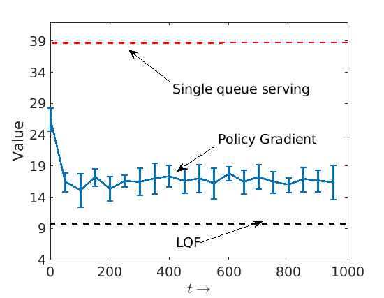
Fig. 5(c) shows the evolution of the value function of GradEst (in blue) compared with those of the base controllers (red) and the Longest Queue First policy (LQF) which, as the name suggests, always serves the longest queue in the system (black). LQF, like any policy that always serves a nonempty queue in the system whenever there is one⁴⁴ 4 Tie-breaking rule is irrelevant., is known to be optimal in the sense of delay minimization for this system [31]. See Sec. F in the Appendix for more details about this experiment.

Finally, Fig. 5(d) shows the result of the second experimental setting with three base controllers, one of which is delay optimal. The first two are $K_{1},K_{2}$ as before and the third controller, $K_{3}$, is LQF. Notice that $K_{1},K_{2}$ are both queue length-agnostic, meaning they could attempt to serve empty queues as well. LQF, on the other hand, always and only serves nonempty queues. Hence, in this case the optimal policy is attained at one of the corner points, i.e., $[0,0,1]$. The plot shows the PG algorithm converging to the correct point on the simplex.

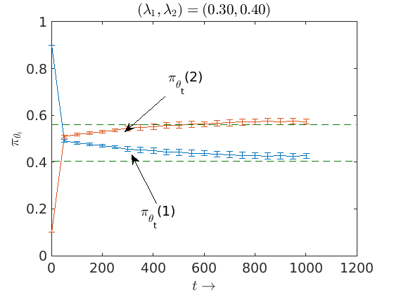
Non-stationary arrival rates. Recall the example that we discussed in Sec. 2.2 of two queues. The scheduler there is now given two base/atomic controllers $\mathcal{C}:=\{K_{1},K_{2}\}$, i.e. $M=2$. Controller $K_{i}$ serves Queue $i$ with probability $1$, $i=1,2$. As can be seen in Fig. 7(b), the arrival rates $\boldsymbol{\lambda}$ to the two queues vary over time (adversarially) during the learning. In particular, $\boldsymbol{\lambda}$ varies from $(0.3,0.6)\to(0.6,0.3)\to(0.49,0.49)$. Our PG algorithm successfully tracks this change and adapts to the optimal improper stationary policies in each case. In all three cases a mixed controller is optimal, and is correctly tracked by our PG algorithm.

Path Graph Networks. Consider a system of parallel transmitter-receiver pairs as shown in Figure  6(a). Due to the physical arrangement of the Tx-Rx pairs, no two adjacent systems can be served simultaneously because of interference. This type of communication system is commonly referred to as a path graph network [32]. Figure  6(b) shows the corresponding conflict graph. Each Tx-Rx pair can be thought of as a queue, and the edges between them represent that the two connecting queues, cannot be served simultaneously. On the other hand, the sets of queues which can be served simultaneously are called independent sets in the queuing theory literature. In the figure above, the independent sets are $\{\emptyset,\{1\},\{2\},\{3\},\{4\},\{1,3\},\{2,4\},\{1,4\}\}$.

The scheduling constraints here dictate that Queues $i$ and $i+1$ cannot be served simultaneously for $i\in[N-1]$ in any round $t\geqslant 0$. In each round $t$, the scheduler selects an independent set to serve the queues therein.

Let $Q_{j}(t)$ be the backlog of Queue $j$ at time $t$. We use the following base controllers: (i) $K_{1}:$ Max Weight (MW) controller [45] chooses a set $s_{t}:=\mathop{\mathrm{argmax}}\limits_{\underline{s}\in\mathcal{A}}\sum\limits_{j\in\underline{s}}Q_{j}(t)$, i.e, the set with the largest backlog, (ii) $K_{2}:$ Maximum Egress Rate (MER) controller chooses a set $s_{t}:=\mathop{\mathrm{argmax}}\limits_{\underline{s}\in\mathcal{A}}\sum\limits_{j\in\underline{s}}\mathbb{I}\{Q_{j}(t)>0\}$, i.e, the set which has the maximum number of non-empty queues.We also choose $K_{3},K_{4}$ and $K_{5}$ which serve the sets $\{1,3\},\{2,4\},\{1,4\}$ respectively with probability 1. We fix the arrival rates to the queues $(0.495,0.495,0.495,0.495)$. It is well known that the MER rule is mean-delay optimal in this case [32]. In Fig. 7(a), we plot the probability of choosing $K_{i},i\in[5]$, learnt by our algorithm. The probability of choosing MER indeed converges to 1.

Finally, in Table 2, we report the mean delay values of the 5 base controllers we used in our simulation Fig. 7(a), Sec.6. We see the controller $K_{2}$ which was chosen to be MER, indeed has the lowest cost associated, and as shown in Fig.  7(a), our Softmax PG algorithm (with estimated value functions and gradients) converges to it.

We consider a linear chain MDP as shown in Figure 8(a). As evident from the figure, $\left|\mathcal{S}\right|=10$ and the learner has only two actions available, which are $\mathcal{A}=\{\tt{left},\tt{right}\}$. Hence the name ‘chain’. The numbers on the arrows represent the reward obtained with the transition. The initial state is $s_{1}$. We let $s_{1}0$ as the terminal state. Let us define 2 base controllers, $K_{1}$ and $K_{2}$, as follows.

References

- [1] Yasin Abbasi-Yadkori and Csaba Szepesvári. Regret bounds for the adaptive control of linear quadratic systems. In Proceedings of the 24th Annual Conference on Learning Theory, volume 19 of Proceedings of Machine Learning Research, pages 1–26, Budapest, Hungary, 09–11 Jun 2011. JMLR Workshop and Conference Proceedings.
- [2] Alekh Agarwal, Sham M Kakade, Jason D Lee, and Gaurav Mahajan. Optimality and approximation with policy gradient methods in markov decision processes. In Proceedings of Thirty Third Conference on Learning Theory, pages 64–66. PMLR, 2020.
- [3] Naman Agarwal, Nataly Brukhim, Elad Hazan, and Zhou Lu. Boosting for control of dynamical systems. In Hal Daumé III and Aarti Singh, editors, Proceedings of the 37th International Conference on Machine Learning, volume 119 of Proceedings of Machine Learning Research, pages 96–103. PMLR, 13–18 Jul 2020.
- [4] P. Auer, N. Cesa-Bianchi, Y. Freund, and R. E. Schapire. Gambling in a rigged casino: The adversarial multi-armed bandit problem. In Proceedings of IEEE 36th Annual Foundations of Computer Science, pages 322–331, 1995.
- [5] Peter Auer, Thomas Jaksch, and Ronald Ortner. Near-optimal regret bounds for reinforcement learning. In Advances in Neural Information Processing Systems, volume 21, pages 89–96. Curran Associates, Inc., 2009.
- [6] Dimitri Bertsekas and Robert Gallager. Data Networks (2nd Ed.). Prentice-Hall, Inc., USA, 1992.
- [7] Dimitri P Bertsekas. Dynamic programming and optimal control 3rd edition, volume ii. Belmont, MA: Athena Scientific, 2011.
- [8] Jalaj Bhandari and D. Russo. Global optimality guarantees for policy gradient methods. ArXiv, abs/1906.01786, 2019.
- [9] Paolo Bolzern, Patrizio Colaneri, and Giuseppe De Nicolao. Almost sure stability of stochastic linear systems with ergodic parameters. European Journal of Control, 14(2):114–123, 2008.
- [10] Vivek S. Borkar. Stochastic Approximation. Cambridge Books. Cambridge University Press, December 2008.
- [11] Asaf Cassel, Alon Cohen, and Tomer Koren. Logarithmic regret for learning linear quadratic regulators efficiently. In Proceedings of the 37th International Conference on Machine Learning, volume 119 of Proceedings of Machine Learning Research, pages 1328–1337. PMLR, 13–18 Jul 2020.
- [12] Xinyi Chen and Elad Hazan. Black-box control for linear dynamical systems. arXiv preprint arXiv:2007.06650, 2020.
- [13] Amit Daniely, Nati Linial, and Shai Shalev-Shwartz. More data speeds up training time in learning halfspaces over sparse vectors. In Advances in Neural Information Processing Systems, volume 26, pages 145–153. Curran Associates, Inc., 2013.
- [14] Amit Daniely, Nati Linial, and Shai Shalev-Shwartz. From average case complexity to improper learning complexity. In Proceedings of the Forty-Sixth Annual ACM Symposium on Theory of Computing, STOC ’14, page 441–448, New York, NY, USA, 2014. Association for Computing Machinery.
- [15] Sarah Dean, Horia Mania, Nikolai Matni, Benjamin Recht, and Stephen Tu. On the Sample Complexity of the Linear Quadratic Regulator. arXiv e-prints, October 2017.
- [16] D. Denisov and N. Walton. Regret analysis of a markov policy gradient algorithm for multi-arm bandits. ArXiv, abs/2007.10229, 2020.
- [17] Rick Durrett. Probability: Theory and examples, 2011.
- [18] Abraham D. Flaxman, Adam Tauman Kalai, and H. Brendan McMahan. Online convex optimization in the bandit setting: Gradient descent without a gradient. SODA ’05, page 385–394, USA, 2005. Society for Industrial and Applied Mathematics.
- [19] Aditya Gopalan and Shie Mannor. Thompson Sampling for Learning Parameterized Markov Decision Processes. In Proceedings of The 28th Conference on Learning Theory, volume 40 of Proceedings of Machine Learning Research, pages 861–898, Paris, France, 03–06 Jul 2015. PMLR.
- [20] Morteza Ibrahimi, Adel Javanmard, and Benjamin Roy. Efficient reinforcement learning for high dimensional linear quadratic systems. In Advances in Neural Information Processing Systems, volume 25, pages 2636–2644. Curran Associates, Inc., 2012.
- [21] Hassan K. Khalil. Nonlinear Control. Pearson, 2015.
- [22] Tomáš Kocák, Gergely Neu, Michal Valko, and Remi Munos. Efficient learning by implicit exploration in bandit problems with side observations. In Advances in Neural Information Processing Systems, volume 27, pages 613–621. Curran Associates, Inc., 2014.
- [23] T.L Lai and Herbert Robbins. Asymptotically efficient adaptive allocation rules. Advances in Applied Mathematics, 6(1):4 – 22, 1985.
- [24] Tor Lattimore and Csaba Szepesvári. Bandit Algorithms. Cambridge University Press, 2020.
- [25] Gen Li, Yuting Wei, Yuejie Chi, Yuantao Gu, and Yuxin Chen. Softmax policy gradient methods can take exponential time to converge. arXiv preprint arXiv:2102.11270, 2021.
- [26] N. Littlestone and M. K. Warmuth. The weighted majority algorithm. Inform. Comput., 108(2):212–261, 1994.
- [27] S Łojasiewicz. Les équations aux dérivées partielles (paris, 1962), 1963.
- [28] Ryan Lowe, Yi Wu, Aviv Tamar, Jean Harb, Pieter Abbeel, and Igor Mordatch. Multi-agent actor-critic for mixed cooperative-competitive environments, 2020.
- [29] Horia Mania, Stephen Tu, and Benjamin Recht. Certainty equivalence is efficient for linear quadratic control. In Advances in Neural Information Processing Systems, volume 32, pages 10154–10164. Curran Associates, Inc., 2019.
- [30] Jincheng Mei, Chenjun Xiao, Csaba Szepesvari, and Dale Schuurmans. On the global convergence rates of softmax policy gradient methods. In Proceedings of the 37th International Conference on Machine Learning, pages 6820–6829. PMLR, 2020.
- [31] A. Mohan, A. Chattopadhyay, and A. Kumar. Hybrid mac protocols for low-delay scheduling. In 2016 IEEE 13th International Conference on Mobile Ad Hoc and Sensor Systems (MASS), pages 47–55, Los Alamitos, CA, USA, oct 2016. IEEE Computer Society.
- [32] Avinash Mohan, Aditya Gopalan, and Anurag Kumar. Throughput optimal decentralized scheduling with single-bit state feedback for a class of queueing systems. ArXiv, abs/2002.08141, 2020.
- [33] Gergely Neu. Explore no more: Improved high-probability regret bounds for non-stochastic bandits. In Advances in Neural Information Processing Systems, volume 28, pages 3168–3176. Curran Associates, Inc., 2015.
- [34] Ian Osband, Daniel Russo, and Benjamin Van Roy. (more) efficient reinforcement learning via posterior sampling. In Advances in Neural Information Processing Systems, volume 26, pages 3003–3011. Curran Associates, Inc., 2013.
- [35] Y. Ouyang, Mukul Gagrani, A. Nayyar, and R. Jain. Learning unknown markov decision processes: A thompson sampling approach. In NIPS, 2017.
- [36] Mircea-Bogdan Radac and Radu-Emil Precup. Data-driven model-free slip control of anti-lock braking systems using reinforcement q-learning. Neurocomput., 275(C):317–329, January 2018.
- [37] G. A. Rummery and M. Niranjan. On-line q-learning using connectionist systems. Technical report, 1994.
- [38] John Schulman, Sergey Levine, Pieter Abbeel, Michael Jordan, and Philipp Moritz. Trust region policy optimization. In Francis Bach and David Blei, editors, Proceedings of the 32nd International Conference on Machine Learning, volume 37 of Proceedings of Machine Learning Research, pages 1889–1897, Lille, France, 07–09 Jul 2015. PMLR.
- [39] John Schulman, Filip Wolski, Prafulla Dhariwal, Alec Radford, and Oleg Klimov. Proximal policy optimization algorithms, 2017.
- [40] Lior Shani, Yonathan Efroni, and Shie Mannor. Adaptive trust region policy optimization: Global convergence and faster rates for regularized mdps. ArXiv, abs/1909.02769, 2020.
- [41] David Silver, Aja Huang, Christopher J. Maddison, Arthur Guez, Laurent Sifre, George van den Driessche, Julian Schrittwieser, Ioannis Antonoglou, Veda Panneershelvam, Marc Lanctot, Sander Dieleman, Dominik Grewe, John Nham, Nal Kalchbrenner, Ilya Sutskever, Timothy Lillicrap, Madeleine Leach, Koray Kavukcuoglu, Thore Graepel, and Demis Hassabis. Mastering the game of go with deep neural networks and tree search. Nature, 529:484–503, 2016.
- [42] Satinder Singh, Andy Okun, and Andrew Jackson. Artificial intelligence: Learning to play Go from scratch. 550(7676):336–337, October 2017.
- [43] Richard S. Sutton and Andrew G. Barto. Reinforcement Learning: An Introduction. The MIT Press, second edition, 2018.
- [44] Richard S Sutton, David McAllester, Satinder Singh, and Yishay Mansour. Policy gradient methods for reinforcement learning with function approximation. In Advances in Neural Information Processing Systems, volume 12, pages 1057–1063. MIT Press, 2000.
- [45] L. Tassiulas and A. Ephremides. Stability properties of constrained queueing systems and scheduling policies for maximum throughput in multihop radio networks. IEEE Transactions on Automatic Control, 37(12):1936–1948, 1992.
Appendix A Glossary of Symbols
- 1.
: State space
- 2.
Action space
- 3.
Cardinality of
- 4.
- 5.
Number of controllers
- 6.
Controller , . For finite SA space MDP, is a matrix of size , where each row is a probability distribution over the actions.
- 7.
Given collection of controllers.
- 8.
Improper policy class setup by the learner.
- 9.
Parameter assigned to the controllers to controllers, representing weights, updated each round by the learner.
- 10.
Probability of choosing controllers
- 11.
Probability of choosing action given state . Note that in our setting, given over controllers (see previous item) and the set of controllers, is completely defined, i.e., . Hence we use simply to denote the policy followed, whenever the context is clear.
- 12.
Immediate (one-step) reward obtained if action is played in state .
- 13.
Probability of transitioning to state from state having taken action .
- 14.
Value function starting with initial distribution over states, and following policy .
- 15.
.
- 16.
- 17.
- 18.
- 19.
. Denotes a distribution over the states, is called the “discounted state visitation measure”
- 20.
- 21.
- 22.
Appendix B Details of simulations settings for the inverted pendulum system
In this section we supply the adjustments we made for specifically for the cartpole experiments. We first mention that we scale down the estimated gradient of the value function returned by the GradEst subroutine (Algorithm 4) (in the inverted pendulum simulation only). The scaling that worked for us is .