Dynamic Virtual Graph Significance Networks for Predicting Influenza
Abstract
Graph-structured data and their related algorithms have attracted significant attention in many fields, such as influenza prediction in public health. However, the variable influenza seasonality, occasional pandemics, and domain knowledge pose great challenges to construct an appropriate graph, which could impair strength of the current popular graph-based algorithms to perform data analysis. In this study, we develop a novel method, Dynamic Virtual Graph Significance Networks (DVGSN), which can supervisedly and dynamically learn from similar “infection situations” in historical timepoints. Representation learning on the dynamic virtual graph can tackle the varied seasonality and pandemics, and therefore improve the performance. The extensive experiments on real-world influenza data demonstrate that DVGSN significantly outperforms the current state-of-the-art methods. To the best of our knowledge, this is the first attempt to supervisedly learn a dynamic virtual graph for time-series prediction tasks. Moreover, the proposed method needs less domain knowledge to build a graph in advance and has rich interpretabilities, which makes the method more acceptable in the fields of public health, life sciences, and so on.
Index Terms:
Representation Learning, Dynamic Virtual Graph, Influenza Prediction, Time Series.I Introduction
With the growing emergence of graph-structured data such as social networks and biological networks [1, 2], the algorithms to analyze graph data have attracted significant attention, such as Graph Convolutional Networks (GCNs) [3, 4, 5] and Graph Attention Networks (GAT) [6], etc. The structure of graph data exerts significant impact on the performance of theses algorithms, because these algorithms heavily depend on the neighborhood relationship of the graph. For example, GNNs iteratively aggregate and integrate the embedding of its neighbors to learn the node embedding of the graph. However, finding out all the influential neighbor nodes and measuring their edge weights appropriately to construct a graph are nontrivial in many cases, such as in life sciences and public health fields, which require substantial domain knowledge.
Influenza prediction is an important interdisciplinary problem between computer science and public health. Influenza circulates worldwide and places a heavy burden on people’s health Every year [7, 8]. The strong infectivity and outbreak of influenza are estimated to result in approximately 35 million cases of symptomatic illnesses, 16 million outpatient medical visits, 490 thousand influenza-associated hospitalizations, and 34 thousand cases of deaths in the influenza season of 2018-2019 in the United States [9]. The influenza virus undergoes high mutation rates and frequent genetic re-assortment [10, 11, 12]. To help clinics, hospitals, pharmaceutical companies, and governments better prepare for influenza in a timely manner, we need a reliable model to predict influenza trends.
There are mainly two challenges of predicting influenza. [Challenge 1] Influenza seasonality usually varies, from one season to another, in timing, severity, and duration [13, 14]. Table I shows the descriptive statistics of the Influenza-Like Illness (ILI) rates of influenza seasons from 2003-2004 to 2016-2017 in the United States. The rates of “standard deviation / mean” in the “Highest ILI Rate” and “Duration” are 33% and 39%, respectively. Such an irregular variation handicaps the predictive methods. [Challenge 2] Influenza pandemics occur occasionally but can totally disorder the seasonality for years. A pandemic is a serious world-wide outburst, resulting from the emerge of a new type of virus and resulting in extremely higher ILI rates, several close and consecutive peaks, and much longer duration, as the piece of the curve around 2009 in Figure 1 shows. Such a “mutated” outbreak makes the prediction more difficult.
| Seasons |
|
|
| ||||||
| 2003-2004 | 2003/06 | 0.0317 | 28 | ||||||
| 2004-2005 | 2003/52 | 0.0706 | 25 | ||||||
| 2005-2006 | 2005/07 | 0.0475 | 37 | ||||||
| 2006-2007 | 2005/52 | 0.0305 | 31 | ||||||
| 2007-2008 | 2007/07 | 0.0327 | 31 | ||||||
| 2008-2009 | 2008/07 | 0.0542 | 31 | ||||||
| 2009-2010 | 2009/06 | 0.0334 | 91 | ||||||
| 2009/21 | 0.0421 | ||||||||
| 2009/42 | 0.0762 | ||||||||
| 2010-2011 | 2011/05 | 0.0444 | 37 | ||||||
| 2011-2012 | 2012/11 | 0.0229 | 41 | ||||||
| 2012-2013 | 2012/52 | 0.0603 | 44 | ||||||
| 2013-2014 | 2013/52 | 0.0439 | 43 | ||||||
| 2014-2015 | 2014/52 | 0.0611 | 41 | ||||||
| 2015-2016 | 2016/10 | 0.0359 | 42 | ||||||
| 2016-2017 | 2017/06 | 0.0481 | 44 | ||||||
| MEAN | - | 0.0460 | 40 | ||||||
|
- | 0.0152 | 16 | ||||||
| SD/MEAN | - | 33% | 39% |

The existing machine/deep learning models, such as XGBoost (XGB), Temporal Pattern Attention Long Short-Term Memory (TPA-LSTM), Temporal Convolutional Networks (TCN), and Transformer, use current and historical values in a user-defined time window as input to predict future values. These methods lack considering similarities outside the time window. Although one can simply increase the length of the time window to include more information, there are always some timepoints outside the window. Besides, the bigger the length of the time window is, the fewer the training instances will be left, which makes the predictive model unreliable. If a method can dynamically find historical timepoints that have similar “infection situations” as auxiliary information, the model could tackle the varied seasonality and the occasional pandemics.
However, how to accurately represent the “infection situations” poses a challenge since the situation should include the information of the influenza severity, the tendency, the duration and other factors that may be beyond our knowledge.

In this study, we develop a novel method, namely Dynamic Virtual Graph Significance Networks (DVGSN), as Figure 2 illustrates. DVGSN constructs a virtual graph for influenza prediction. In the virtual graph, a virtual node represents a timepoint. The embedding of a virtual node represents the “infection situations” at the timepoint. The virtual edges connect two virtual nodes at two timepoints, and the edge weights measure the significance of the virtual edge. Since the timepoints connected by the virtual edges can be outside the time window, DVGSN can break the limitation of the time window by learning from neighbor nodes and improve the predictive accuracy.
A natural static graph defined with domain knowledge beforehand could not align well with the specific analytical task. As a result, the “neighborhood” in an “unsupervised graph” could be improper for the specific analytical task and damage the analytical outcomes. Different from a natural graph with static nodes and edges, in a dynamic virtual graph, every node and edge are supervisedly dynamically learned during the training procedure in the prediction task. Moreover, a virtual graph naturally has rich interpretabilities. For example, similar “infection situations” found by the virtual graph can provide us with clues how the virtual graph finds similarities and how the proposed method performs the prediction for pandemics. The interpretabilities make the proposed method more acceptable, especially in the fields of epidemiology and public health, in which researches usually emphasize the interpretabilities of the predictive models for further government measures, etc.
The contributions of this work are concluded as follows.
(1) To the best of our knowledge, this is the first attempt to supervisedly learn a dynamic virtual graph for time-series prediction.
(2) The proposed method need less domain knowledge to build a graph in advance and has rich interpretabilities, which are indispensable in epidemiology, public health, and the like.
(3) We carry out extensive experiments on the real-world data, and the experimental results prove that the proposed method significantly outperforms the state-of-the-art methods.
II RELATED WORK
This section describes the previous work from the point of view of influenza prediction and graph-based deep learning.
II-A Influenza Prediction
The machine/deep learning for forecasting influenza or other time-series data are mainly categorized into two groups. Firstly, some researchers focus on looking for effective “features”. For example, search engine query data are used for prediction influenza in Google Flu Trends11 1 https://www.google.org/flutrend [15, 16]. Twitter data are also used in other research papers [17, 18]. However, these models usually suffer from the unreliable source of huge amounts of information from such as internet searches. For example, Google’s algorithm was quite vulnerable to overfitting to seasonal terms unrelated to the flu, like “high school basketball”. This example also demonstrates the importance of model interpretability. Secondly, other researchers focus on looking for effective “models”, such as RF [19, 20, 21], Gradient Boosting [19, 21], Multilayer Perceptron (MLP) [19, 21], Long Short Term Memory (LSTM) [19, 21, 22], Transformer (TFR) [23], and so on. Deep learning based methods, e.g. Transformer, are drawing more attention for their accuracy while most of them suffers from the poor interpretability.
Moreover, statistical models and dynamic analysis models are considered easily accessible tools for simulating patterns of infection by influenza, such as SI, SIS, SIR model and their variants [24]. However, their parameters are subject to change and the approximation of the parameters is difficult [25], such as the basic reproduction number , population mobility etc.
II-B Graph-based deep learning
For mining a natural graph, such as Cora [26] and Digg [27], Graph Neural Networks (GNNs) are usually used, such as GCN, GAT, and Graph Isomorphism Network (GIN) [28]. In an analytical task without a natural graph, to leverage powerful GNNs, a graph can be constructed beforehand. Researches need to use domain knowledge, such as medicine and transportation [29], and mathematical calculation, such as Euclidean distance [30], to construct a graph beforehand. Nonetheless, all of these graphs are thought of as “unsupervised graphs” because the calculation for the construction is not updated by backpropagation for the specific analytical task. In other words, an “unsupervised graph” could NOT align with the specific analytical task. As a result, the “neighborhood” in an “unsupervised graph” could be improper for the specific analytical task and damage the analytical outcomes. In this study, we develop a method to construct a “supervised graph”, which could dynamically and supervisedly learn the effective information from other instances during the training procedure in the specific analytical task.
III THE PROPOSED MEHTOD
III-A Influenza prediction tasks
We formally define the prediction task with the classic machine/deep learning algorithms as Formula 1:
| (1) |
where is the vector to be predicted, is a given timepoint, and is the predictive window size; is the predicted value of the upcoming -th week, and is a time-series model to predict the value of the upcoming -th week; is the observed time-series values with a time lag , is the observed value, and is the value of the past -th week.
There are two types of time-series prediction: (a) single-step influenza prediction and (b) multi-step prediction. A single-step prediction predicts the value for one step in advance ( in Formula 1 ), and a multi-step prediction predicts the consecutive values with a bigger predictive window size ( in Formula 1).
As Formula 1 shows, the classic methods heavily depends on the observations in the time window but lacks considering historical similarities outside the time window. Table II presents the notations utilized in this work.
| Notations | Explanations | ||
|---|---|---|---|
| the observed time-seies data | |||
| the time lag | |||
| the predictive window size | |||
| |||
| |||
| the virtual graph | |||
| the set of all virtual nodes | |||
| the set of all virtual edges | |||
| the observed matrix of the ILI rates | |||
| the node embedding matrix of the virtual graph | |||
| the adjacency matrix of the virtual graph |
III-B Dynamic Virtual Graph
As aforementioned in Table 1 and Figure 1, Influenza seasons that vary in timing, severity, and duration. And pandemics mutate the influenza outbreaks. Dynamically looking for similar “infection situations” instead of sticking to a fixed periodicity (roughly one year) could be a key to varied seasonality and pandemics for influenza prediction. We formally define the concept of a dynamic virtual graph.
Dynamic Virtual Graph. Different from a natural graph with static nodes and edges, we define a virtual graph as with a set of nodes () and a set of edges (), in which every node and edge are supervisedly or semi-supervisedly dynamically learned during the training procedure in the prediction task.

In this study each node is a function that can be trained to capture “infection situations”, and each edge describes the significance of the similarity. Figure 3 gives an image of a virtual graph to predict influenza in this study. A virtual node () represents a timepoint, such as 2017/12, which means the 12th week in 2017. The embedding of the virtual node, representing the comprehensive “infection situations” at the timepoint, is denoted as for the node . A virtual edge () connects two virtual nodes at two timepoints, and the edge weights measure the significance of the virtual edge.
III-C Virtual Node Representation
The virtual node representation will be used (1) to perform “infection-situations” embedding for the subsequent representation learning and (2) to learn the significance of the similarity among the different “infection-situations”. How to define a proper function of the virtual node representation vector for the node is a pivotal problem. An “infection-situation” embedding vector needs to include comprehensive infective information, such as :
(a) the timing, severity, and duration of the infection at a given timepoint;
(b) the first-order differences (“speed”) and the second-order differences (“acceleration”) at a given timepoint;
(c) tendency (upward, downward, fluctuation, or a turning point) at a given timepoint;
(d) descriptive statistics (mean, median, maximum, minimum, variance, and the like) at a given timepoint.
Many previous researches studied how to “unsupervisedly” represent “situation” for prediction [31, 32, 33, 34]. Some use current and past values in the time-series data as input. Others use domain knowledge, such as varying lag structures at different steps [32], to present “situation” vectors. Nonetheless, these methods of “unsupervised presenting” is separate from the model training. In this study, we propose a supervised representation of “situation” to learn a more appropriate presentation for a given analytical task. Formula 2 illustrates the node representation of “infection-situations”:
| (2) |
where is a neural network, is the parameter for (), and is an activation function for which we use Exponential Linear Units (ELU) in this work. In this work, a two-layered Multilayer Perceptron (MLP) is adopted. and are the trainable weights of the first and second layer of MLP, respectively.
There are three reasons why we need to project the original feature space nonlinearly into a high-dimensional space as an embedding vector of a virtual node:
(a) To work as time-series feature extraction.
Time-series analyses usually adopt arbitrary feature engineering, such as Kalman Filtering [35], and so on. How to select effective feature engineering is non-trivial, usually experienced-based and time-consuming. Since an MLP can theoretically simulate any function [36, 37, 38], implementing MLP can perform effective representation in a high-dimensional space.
(b) To supervisedly and dynamically learn virtual node representations.
Since the MLP is a part of the entire end-to-end learning, the projected embedding vectors are supervisedly learned from and for a specific analytical task. Such a supervisedly-learned embedding space is supposed to work better than the original feature space, which is static and cannot be updated or learned, and thereby improve the accuracy.
(c) To project virtual node embedding to an appropriate space.
The high-dimensional embedding vectors of two virtual nodes will be used to define the significance of a virtual edge. A high-dimensional space that represents a variety of complex time-series characteristics can work better than the original feature space that just consists of the ILI rates of current and past few weeks.
III-D Virtual Edge Significance
To a given node, different neighbors may have different similarities in “infection situations”. The significance of a virtual edge needs to be decided. In this study, we measure the significance of the virtual edge between the node and by performing inner product on the after linear projection and instance normalization on the high-dimensional embedding vectors of “infection-situations”, as Formula 3 illustrates:
| (3) |
where is the the significance of the virtual edge from the node to , is the instance normalization, is the trainable weight of the linear projection and is the inner product.
The significance () of the virtual edge from the node to has some properties:
(a)
The value range of virtual edge significance is .
(b)
The significance of the self-loop virtual edge is “1”.
(c)
The virtual edge significance is symmetric.
III-E Graph Significance Networks
The virtual graph, which is composed of the virtual nodes representing the “infection situation” at each timepoint and the virtual edges with the similarity significance, is input into GNNs. For a given node, the GNNs iteratively aggregate and integrate the embedding of its neighbors to learn a representation vector (). Formula 4 illustrates the -th iteration of aggregation and integration:
| (4) |
where and is the representation vector at the -th iteration/layer of the given node and the neighbor node , respectively; is the set of neighbor nodes; is a function that aggregates the infective information from its neighbors —the timepoints that have similar “infection situations”, and is a function that integrates the infective information from the given timepoint itself and the aggregated infective information by based on its neighbors .
III-F Regressive Layer
The sum of the initial virtual node representation (), the representation vector after the first GNN layer (), and the second GNN layer () is input into a regressive layer (implemented by a linear layer) to achieve the final prediction, as Formula 6 shows:
| (6) |
where is the trainable weight of the final regressive layer.
III-G Loss Function
The loss function is defined as Formula 7 shows:
| (7) |
where is the predictive loss in Mean Square Error (MSE) ( is the number of virtual nodes), and are the vectors of the true and predicted values, respectively. is the adjacency matrix of the virtual graph, and is the penalty term to limit the complexity of the virtual graphs and improve the robustness of the model, and represents the matrix Frobenius norm); and is an adjustable hyper-parameter to balance the two parts of losses.

III-H Comparison with the existing methods
(a) The limitation of time window
The prediction for a given timepoint by DVGSN can be simplified and formularized as Formula 8:
| (8) |
where is the algorithm of DVGSN and represents the set of all the parameters in DVGSN.
To perform prediction for the timepoint , all the observed time-series data () in the training dataset are input into DVGSN. Comparatively, the input in the classic machine/deep learning methods (as formula 1 shows) are just the observed values () in the user-defined time window with the time lag (). Inputting all the observed time-series data () can capture similar “infection situations” from all the timepoints instead of sticking to the fixed static nodes and edges.
(b) Other differences
The virtual nodes and virtual edges in DVGSN are supervisedly learned during the training procedure in the specific prediction task while the other existing GNNs-based methods use a static graph defined beforehand. Another difference lies in the function in Formula 4. The algorithm of the -th layer of iteration in the attentive GNNs (such as GAT) and DVGSN is illustrated as Formula 9 and Formula 10 shows, respectively:
| (9) |
where is the normalized attention coefficient, represents matrix transposition, and is the concatenation operation.
| (10) |
In GAT, the input () is a (precisely a weighted ) of the embedding vectors in the neighborhood since regardless of the graph structure. Comparatively, in DVGSN, the aggregation function is a of the embedding vectors in the neighborhood on condition that holds. Theoretically, the expressive power of based aggregators is weaker than aggregators because captures the full multiset while captures the proportion / distribution of elements of a given type [28].
IV EXPERIMENTS
IV-A Data
We scrape the influenza data of the United States from 2003/30 to 2017/30 in the “FluView Interactive” [39], a website of Centers for Disease Control and Prevention, National Center for Immunization and Respiratory Diseases. The weekly ILI rates are calculated and used for this work. Figure 1 illustrates the time-series plot of the ILI rates. The piece of the curve around 2009, which has three consecutive peaks, is a pandemic in 2009. Table I summaries the descriptive statistics of the influenza seasons from 2002-2003 to 2016-2017. The “mean standard deviation” of the column of “The Highest ILI Rate” is . Besides, the standard deviation () is around 33% higher than the value of mean (), presenting a considerable variance in severity. The “mean standard deviation” of the column of “Duration” is . The standard deviation () is around 40%h of the mean (), presenting a considerable variance in lasting. Moreover, the column of “The Peak week” demonstrates the timing of influenza seasons varies year by year.
IV-B Baseline
In this work, the baseline models include a variety of state-of-the-art models. We do not compare with the SI-based models because it is difficult to obtain the values of the parameters such as the number of susceptible and infected individuals.
Autoregression (AR). An AR model is a statistical method that uses observed values from current and past time steps as input and implements a linear regression to predict future values.
-Nearest Neighbors(-NN). The regression of -NN examines the values of a chosen number () of data points surrounding a target data point, and uses the mean of the values as prediction. The -NN regression can be used for time-series prediction [40].
Random Forest(RF). A RF model is an ensemble of decision trees trained with the “bagging” method, which leverages a combination of learning models and thereby increases the overall performance [41].
XGB. The XGB regression implements the framework of Gradient Boosting by providing a parallel boosting, which consists of iteratively learning weak regressors with respect to a distribution and adding them to a final strong regressor [42].
Multilayer Perceptron (MLP). An MLP is a neural network, in which each node in a layer is fully connected to every node in the adjacent layers and fit a non-linear function. The MLP can be used for time series analyses by mapping current and past values to one or multiple future predictive values [43].
TPA-LSTM. The TPA-LSTM uses a set of filters to extract time-invariant temporal patterns. The extraction is similar to transforming time series data into its “frequency domain” for forecasting [44].
TCN. A TCN uses a causal and dilated convolutional network to predict sequential data [45], such as time series [46], and so on .
TFR. The TFR is a model relying entirely on attention mechanism to compute representations of its input and output without using sequence aligned RNNs or convolution [47]. TFR can also be used for time -series prediction [48].
GAT. The GAT algorithm is a type of GNNs that considers the attention mechanism on graphs [6].
GIN. The GIN model is a theoretically designed model for analyzing the expressive power of GNNs to capture different graph structures. The GIN is provably the most expressive among the class of GNNs and is theoretically as powerful as the Weisfeiler-Lehman graph isomorphism test [28].
IV-C Implementation Details
For all the baseline models and the proposed model, we randomly initialize parameters with the uniform distribution and select the Adam optimizer[49] with a learning rate of 0.001. We set all hidden layer size of 256 units and use the activation function of an ELU. We set the epoch to 200 and choose the parameter with the best result on the validation set. To ensure fairness, we split the datasets and use the same training set (the current timepoints are from 2003/41 to 2012/02), validation set (the current timepoints are from 2012/03 to 2014/42), and testing set (the current timepoints are from 2014/43 to 2017/29 when the predictive window size is 1; the current timepoints are from 2014/43 to 2017/27 when the predictive window size is 3; the current timepoints are from 2014/43 to 2017/24 when the predictive window size is 6) for all the models in this work. We set all the models to the same depth. For MLP, we use a five-layer structure, which contains an input layer, four hidden layers, and an output layer (regressive layer). For TPA-LSTM, we feed the feature vectors into a TPA-LSTM layer, then input the hidden state to 3-layered MLP, and finally implement an output layer. For TFR, we use two TFR blocks, which correspond to four layers. For GAT, we use four layers of GAT and one output layer. For the proposed method, in each backpropagation, we use all training data as model input and randomly select batch nodes from the training set to calculate the loss and update model parameters. In this work, to use the algorithm of GIN and GAT, we also connect a given virtual node to all the other virtual nodes, as DVGSN does. Our source code and dataset are available at https://github.com/aI-area/DVGSN.
IV-D Results
| p ∗ | q ∗ | AR | kNN | RF | XGB | MLP | TPA-LSTM | TCN | TRF | GAT | GIN | DVGSN |
|---|---|---|---|---|---|---|---|---|---|---|---|---|
| 6 | 1 | 0.0796 | 0.1177 | 0.0897 | 0.1071 | 0.0795 | 0.0774 | 0.0794 | 0.0867 | 1.2326 | 1.1891 | 0.0749 |
| 3 | - | 0.2750 | 0.2223 | 0.2586 | 0.2106 | 0.2103 | 0.2101 | 0.2254 | 1.2228 | 1.2959 | 0.1765 | |
| 6 | - | 0.4258 | 0.3723 | 0.3875 | 0.2976 | 0.3296 | 0.2801 | 0.3984 | 1.2239 | 1.2858 | 0.2770 | |
| 9 | 1 | 0.0787 | 0.1996 | 0.0978 | 0.1138 | 0.0868 | 0.0806 | 0.0884 | 0.0995 | 1.2286 | 0.9772 | 0.0696 |
| 3 | - | 0.3512 | 0.2183 | 0.2523 | 0.2171 | 0.1965 | 0.2112 | 0.2512 | 1.2264 | 1.2056 | 0.1692 | |
| 6 | - | 0.4942 | 0.3330 | 0.3743 | 0.2982 | 0.4093 | 0.3081 | 0.3422 | 1.2231 | 3.3885 | 0.2542 | |
| 12 | 1 | 0.0778 | 0.2113 | 0.0844 | 0.0916 | 0.0878 | 0.0799 | 0.0840 | 0.0930 | 1.2299 | 1.2733 | 0.0691 |
| 3 | - | 0.3625 | 0.1839 | 0.1985 | 0.2116 | 0.1944 | 0.2099 | 0.2706 | 1.2282 | 1.4313 | 0.1692 | |
| 6 | - | 0.4880 | 0.2941 | 0.3239 | 0.2878 | 0.3850 | 0.3209 | 0.3262 | 1.2085 | 1.6453 | 0.2695 |
- •
∗ The p and q refers to the time lag and the predictive window size, respectively.
To perform a comprehensive comparison, we perform three series of experiments. We set the the predictive window size to 1 to do a short period prediction, and set the value to be 3 and 6 respectively to test the predictive ability in a longer period. The loss functions of all the models average the predictive MSEs of the future weeks. To evaluate the robustness of the model, we also test each algorithm with a time lag of 6, 9, and 12, respectively. The value of in this group of experiments is 0.01.
Table III presents the results of all the models. The results show that the proposed DVGSN significantly outperforms all the baseline methods in all the prediction tasks with the predictive window size being 1, 3 and 6 respectively, which proves that DVGSN can satisfy both the short and long period prediction tasks.
Time lag. DVGSN shows a slight advantage with the time lag being 9. The results shows that it is better enough to construct the virtual graph node and reflect the current trend with the recent 9 historical data. A longer time lag may offer no help since the virtual graph can learn the similar historical situation by itself. The result also shows that the selection of the hyperparameter time lag for DVGSN is relatively easy.
The other baseline methods, including KNN, RF, XG, MLP, and TPA-LSTM shows a better performance with a short time lag 6 for the short period prediction as the predictive window size is 1, while a bigger time lag 12 is better for a longer period prediction task in which the predictive window size is 3. A longer time lag could offer more support for the longer prediction task. However, as we have introduced previously, the time lag is limited and a longer one can reduce the training space.
The situation of TCN, TFR, GAT and GIN is more like a comprise between the above two cases. They show a better performance with a short time lag 6 for the short period prediction while a slight advantage with the time lag being 9 for the longer prediction task. The graph-based solutions could reduce their dependence on the time lag. At the same time, the fact that they cannot benefit from a longer time lag for the short prediction may be caused by their fixed static graph mode.
V Ablation Study
To verify the effectiveness of the constructed dynamic graph, we designed a variant, denoted as “DVGSN(fixed)”, in which the virtual edges are fixed instead of being learned. A given node is connected to the nodes at the timepoints one week ago and one year (52 weeks) ago, considering the periodicity and time series of influenza. Other preprocesses are the same as those in the proposed method. We aslo adjust the hyperparameter to demonstrate the effectiveness of the penalty term in the loss function.
| q | 1 | 3 | 6 | ||||||||
|---|---|---|---|---|---|---|---|---|---|---|---|
| p | 6 | 9 | 12 | 6 | 9 | 12 | 6 | 9 | 12 | ||
|
0.0712 | 0.0773 | 0.0709 | 0.1817 | 0.1749 | 0.1780 | 0.3043 | 0.2699 | 0.2749 | ||
|
0.0749 | 0.0696 | 0.0691 | 0.1765 | 0.1692 | 0.1692 | 0.2770 | 0.2542 | 0.2695 | ||
| q | p | ||||||||||
|---|---|---|---|---|---|---|---|---|---|---|---|
| 1 | 6 | 0.0734 | 0.0763 | 0.0800 | 0.0700 | 0.0696 | 0.0749 | 0.0714 | 0.0705 | 0.0765 | 0.0710 |
| 1 | 9 | 0.0699 | 0.0657 | 0.0792 | 0.0751 | 0.0713 | 0.0696 | 0.0710 | 0.0735 | 0.0685 | 0.0698 |
| 1 | 12 | 0.0676 | 0.0898 | 0.0709 | 0.0712 | 0.0684 | 0.0691 | 0.0792 | 0.0759 | 0.0771 | 0.0775 |
| 3 | 6 | 0.1900 | 0.1874 | 0.1804 | 0.1875 | 0.1795 | 0.1765 | 0.1790 | 0.1772 | 0.1789 | 0.1888 |
| 3 | 9 | 0.1742 | 0.1777 | 0.1752 | 0.1779 | 0.1672 | 0.1692 | 0.1771 | 0.1739 | 0.1750 | 0.1708 |
| 3 | 12 | 0.1750 | 0.1873 | 0.1787 | 0.1699 | 0.1788 | 0.1692 | 0.1760 | 0.1727 | 0.1758 | 0.1777 |
| 6 | 6 | 0.2777 | 0.2758 | 0.2745 | 0.2964 | 0.2797 | 0.2770 | 0.2824 | 0.2765 | 0.3035 | 0.3082 |
| 6 | 9 | 0.3330 | 0.2797 | 0.2729 | 0.2626 | 0.2664 | 0.2542 | 0.2759 | 0.2767 | 0.2746 | 0.2962 |
| 6 | 12 | 0.2381 | 0.2376 | 0.2702 | 0.2531 | 0.2507 | 0.2695 | 0.2509 | 0.2675 | 0.2702 | 0.2618 |
Comparison between the fixed and dynamic graph. Table IV compares the performance of the fixed and dynamic graph. In 8 of 9 cases, the dynamic graphs perform better.
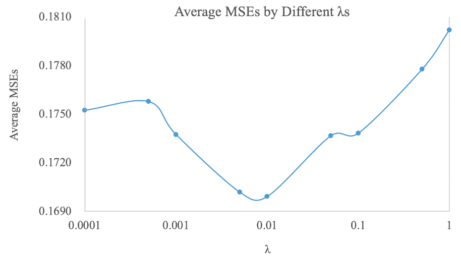
Comparison among different s in DVGSN. A bigger exerts a heavier penalty on a complex virtual graphs with dense edges of small weights. Table V shows comparison among different s in DVGSN. In the most cases, the “DVGSN ()” outperforms the “DVGSN ()”. In conclusion, restricting the complexity of the virtual graph improves the performance.
Figure 5 compares the average MSEs by the different s. The X-axis and Y-axis represents s in logarithm scale and the column-average MSEs from Table V, respectively. The curve roughly presents a shape of the letter of “V”. That is probably because the penalty term cannot help to improve the robustness when the is too small (close to zero). When the is too big, the loss will focus on the penalty term but ignore the predictive MSE loss. In a word, in this work, when the approximately equals to 0.01, DVGSN performs best.


VI Model Interpretation
This section explains how the proposed method works.
VI-A How does DVGSN learn the significance of the similarity?
Figure 6 illustrates the similarity that the virtual graph learns. The X-axis represents the time series from the past 11th week to the future 3rd week ( and ). The Y-axis represents the ILI rate. The date in the format of “year/week” above each column of the subfigures is the “current” timepoint. The model predicts the ILI rates of the future 3 weeks (on the right side of the red dash line). In each subfigure, the red curves represent the “infection situations” of the given timepoints. The ILI rates of the current and past 11 weeks (on the left side of the red dash line) are projected to a high-dimensional space to calculate the significance of the similarity (the green float in each subfigure). As a result, the blue curves in the top two subfigures are the most positively similar “infection situations” that the virtual graph finds; the blue curves in the third row of the subfigure represent dissimilar “infection situations” that the virtual graph finds; and the blue curves in the bottom two subfigures are the most negatively similar “infection situations” that the virtual graph finds.
VI-B How does DVGSN learn for the varied seasonality?
This section explores whether DVGSN can deal with the varied influenza seasonality. Figure 7 gives two examples. The X-axis represents the time series from the past 9th week to the upcoming 3rd week ( and ). The red curves represent the “infection situations” of the given timepoints; and the blue and green curves represent the two most similar “infection situations”. We find the two most similar timepoints do not correspond to the same week of the previous years, which demonstrates DVGSN can tackle varied influenza seasonality instead of sticking to the periodicity of 52 weeks.
VI-C How does DVGSN learn for the pandemic?
This section explores how DVGSN learns from the historical “infection situations” and predicts the pandemic. We present five examples in the 2009 pandemic in Figure 8. The X-axis and Y-axis represents time series from 2002/40 to 2017/30 and the ILI rates, respectively. In each subfigure, the red piece represents the “infection situations” of the given timepoints in the pandemic. The timepoints in the five subfigures is 2009/07, 2009/13, 2009/37, 2009/51, and 2010/11 respectively, which represent a rising, a falling down, a rebound after reaching a bottom, a drop after reaching a peak, and fluctuations after a huge dropping in the 2009 pandemic respectively. The two yellow pieces in the curves represent two of the most similar “infection situations” that DVGSN learns. The number after “w:” in each figure legend is the significance of the similarity. By comparing the past “infection situations” and future tendency between the red pieces and the two yellow pieces in the five examples, we conclude that DVGSN can find and learn the similar “infection situations” outside the pandemic and thereby make a reliable model for the influenza prediction.
VII Conclusion
In this work, we proposed a method—DVGSN. DVGSN can find similar “infection situations” outside the time window and therefore improve the predictive accuracy for influenza. The extensive experiments on real-world influenza data demonstrate that DVGSN significantly outperforms the current state-of-the-art methods. Besides, the proposed method has rich interpretabilities, which provide us clues how the model perform prediction for influenza. Another strong point of the proposed method lies in that it need less domain knowledge to build a graph in advance, which may be very difficult in the medical science related fields. As all the deep learning based methods the proposed method also depends on enough data to train the model. Hopefully, this method can help us better prepare for influenza outbreaks, and work on other public health related analytical tasks well.
Acknowledgments
This work was supported by the Strategic Priority Research Program of Chinese Academy of Sciences (Grant No. XDB38040200). We would like to thank all the authors of the open source code in the baseline methods.
References
- [1] A. Lancichinetti, F. Radicchi, J. J. Ramasco, and S. Fortunato, “Finding statistically significant communities in networks,” PloS one, vol. 6, no. 4, 2011.
- [2] W. W. Zachary, “An information flow model for conflict and fission in small groups,” Journal of anthropological research, vol. 33, no. 4, pp. 452–473, 1977.
- [3] J. Bruna, W. Zaremba, A. Szlam, and Y. LeCun, “Spectral networks and locally connected networks on graphs,” arXiv preprint arXiv:1312.6203, 2013.
- [4] M. Defferrard, X. Bresson, and P. Vandergheynst, “Convolutional neural networks on graphs with fast localized spectral filtering,” in Advances in neural information processing systems, 2016, pp. 3844–3852.
- [5] T. N. Kipf and M. Welling, “Semi-supervised classification with graph convolutional networks,” arXiv preprint arXiv:1609.02907, 2016.
- [6] P. Veličković, G. Cucurull, A. Casanova, A. Romero, P. Lio, and Y. Bengio, “Graph attention networks,” arXiv preprint arXiv:1710.10903, 2017.
- [7] H. Influenza, “Key facts about influenza (flu) vaccine,” Influenza Human, 2005.
- [8] G. Brankston, L. Gitterman, Z. Hirji, C. Lemieux, and M. Gardam, “Transmission of influenza a in human beings.” vol. 7, no. 4, p. 257, 2007.
- [9] C. for Disease Control, N. C. f. I. Prevention, and R. D. (NCIRD), “Disease burden of influenza,” 2020. [Online]. Available: https://www.cdc.gov/flu/about/season/flu-season-2015-2016.htm
- [10] M. D. Lubeck, J. L. Schulman, and P. Palese, “Antigenic variants of influenza viruses: Marked differences in the frequencies of variants selected with different monoclonal antibodies,” vol. 102, no. 2, pp. 458–462.
- [11] J. Stech, X. Xiong, C. Scholtissek, and R. G. Webster, “Independence of evolutionary and mutational rates after transmission of avian influenza viruses to swine,” Journal of Virology, vol. 73, no. 3, pp. 1878–1884, 1999.
- [12] P. Suárez, J. Valcárcel, and J. Ortín, “Heterogeneity of the mutation rates of influenza a viruses: Isolation of mutator mutants,” Journal of Virology, vol. 66, no. 4, pp. 2491–2494, 1992.
- [13] J. Puig-Barberà, A. Tormos, A. Sominina, E. Burtseva, O. Launay, M. A. Ciblak, A. Natividad-Sancho, A. Buigues-Vila, S. Martínez-úbeda, and C. Mahé, “First-year results of the global influenza hospital surveillance network: 2012–2013 northern hemisphere influenza season,” BMC Public Health, vol. 14, no. 1, p. 564.
- [14] C. for Disease Control, N. C. f. I. Prevention, and R. D. (NCIRD), “Summary of the 2015-2016 influenza season,” 2016. [Online]. Available: https://www.cdc.gov/flu/about/season/flu-season-2015-2016.htm
- [15] J. GINSBERG, “Detecting influenza epidemics using search engine query data,” Nature, vol. 457, 2009.
- [16] K. Lee, A. Agrawal, and A. Choudhary, “Forecasting influenza levels using real-time social media streams,” in 2017 IEEE International Conference on Healthcare Informatics (ICHI), 2017.
- [17] S. Molaei, M. Khansari, H. Veisi, and M. Salehi, “Predicting the spread of influenza epidemics by analyzing twitter messages,” Health and Technology.
- [18] J. Li and C. Cardie, “Early stage influenza detection from twitter,” Computer Science, 2013.
- [19] A. Darwish, Y. Rahhal, and A. Jafar, “A comparative study on predicting influenza outbreaks using different feature spaces: application of influenza-like illness data from early warning alert and response system in syria,” BMC Research Notes, vol. 13, no. 1, pp. 1–8, 2020.
- [20] M. J. Kane, N. Price, M. Scotch, and P. Rabinowitz, “Comparison of arima and random forest time series models for prediction of avian influenza h5n1 outbreaks,” Bmc Bioinformatics, vol. 15, no. 1, pp. 276 (9 pp.)—276 (9 pp.).
- [21] J. Zhang and K. Nawata, “A comparative study on predicting influenza outbreaks,” Bioscience trends, 2017.
- [22] R. Yin, E. Luusua, J. Dabrowski, Y. Zhang, and C. K. Kwoh, “Tempel: Time-series mutation prediction of influenza a viruses via attention-based recurrent neural networks,” Bioinformatics, 2020.
- [23] N. Wu, B. Green, X. Ben, and S. O’Banion, “Deep transformer models for time series forecasting: The influenza prevalence case,” arXiv preprint arXiv:2001.08317, 2020.
- [24] V. Dukic, H. F. Lopes, and N. G. Polson, “Tracking epidemics with google flu trends data and a state-space seir model,” Journal of the American Statistical Association, vol. 107, 2012.
- [25] Q. Wu, X. Fu, Z. Jin, and M. Small, “Influence of dynamic immunization on epidemic spreading in networks,” Physica A Statistical Mechanics & Its Applications, vol. 419, pp. 566–574.
- [26] P. Sen, G. Namata, M. Bilgic, L. Getoor, B. Galligher, and T. Eliassi-Rad, “Collective classification in network data,” AI magazine, vol. 29, no. 3, pp. 93–93, 2008.
- [27] T. Hogg and K. Lerman, “Social dynamics of digg,” EPJ Data Science, vol. 1, no. 1, p. 5, 2012.
- [28] K. Xu, W. Hu, J. Leskovec, and S. Jegelka, “How powerful are graph neural networks?” arXiv preprint arXiv:1810.00826, 2018.
- [29] X. Geng, Y. Li, L. Wang, L. Zhang, Q. Yang, J. Ye, and Y. Liu, “Spatiotemporal multi-graph convolution network for ride-hailing demand forecasting,” in Proceedings of the AAAI Conference on Artificial Intelligence, vol. 33, 2019, pp. 3656–3663.
- [30] S. Fu, X. Yang, and W. Liu, “The comparison of different graph convolutional neural networks for image recognition,” in Proceedings of the 10th International Conference on Internet Multimedia Computing and Service, 2018, pp. 1–6.
- [31] J. Alberg and Z. C. Lipton, “Improving factor-based quantitative investing by forecasting company fundamentals,” arXiv preprint arXiv:1711.04837, 2017.
- [32] S. F. Crone and S. Häger, “Feature selection of autoregressive neural network inputs for trend time series forecasting,” in 2016 International Joint Conference on Neural Networks (IJCNN). IEEE, 2016, pp. 1515–1522.
- [33] R. J. Frank, N. Davey, and S. P. Hunt, “Time series prediction and neural networks,” Journal of intelligent and robotic systems, vol. 31, no. 1-3, pp. 91–103, 2001.
- [34] M. Ghiassi, H. Saidane, and D. Zimbra, “A dynamic artificial neural network model for forecasting time series events,” International Journal of Forecasting, vol. 21, no. 2, pp. 341–362, 2005.
- [35] I. K. F. Links, “An introduction to the kalman filter,” 1995.
- [36] K. Hornic, “Multilayer feedforward networks are universal approximators,” vol. 2, no. 5, pp. 359–366, 1989.
- [37] M. Leshno, V. Y. Lin, A. Pinkus, and S. Schocken, “Multilayer feedforward networks with a nonpolynomial activation function can approximate any function,” Neural Networks, vol. 6, no. 6, pp. 861–867.
- [38] K. Hornik, “Approximation capabilities of multilayer feedforward networks,” Neural Networks, vol. 4, no. 2, pp. 251–257.
- [39] C. for Disease Control, N. C. f. I. Prevention, and R. D. (NCIRD), “Fluview interactive,” 2018. [Online]. Available: https://www.cdc.gov/flu/weekly/fluviewinteractive.htm
- [40] S. Mehdizadeh, “Using ar, ma, and arma time series models to improve the performance of mars and knn approaches in monthly precipitation modeling under limited climatic data,” Water Resources Management, vol. 34, no. 1, pp. 263–282, 2020.
- [41] H. Wu, Y. Cai, Y. Wu, R. Zhong, Q. Li, J. Zheng, D. Lin, and Y. Li, “Time series analysis of weekly influenza-like illness rate using a one-year period of factors in random forest regression,” Bioscience trends, 2017.
- [42] R. A. Abbasi, N. Javaid, M. N. J. Ghuman, Z. A. Khan, S. U. Rehman et al., “Short term load forecasting using xgboost,” in Workshops of the International Conference on Advanced Information Networking and Applications. Springer, 2019, pp. 1120–1131.
- [43] J. Cao, Z. Li, and J. Li, “Financial time series forecasting model based on ceemdan and lstm,” Physica A: Statistical Mechanics and its Applications, vol. 519, pp. 127–139, 2019.
- [44] S.-Y. Shih, F.-K. Sun, and H.-y. Lee, “Temporal pattern attention for multivariate time series forecasting,” Machine Learning, vol. 108, no. 8-9, pp. 1421–1441, 2019.
- [45] S. Bai, J. Z. Kolter, and V. Koltun, “An empirical evaluation of generic convolutional and recurrent networks for sequence modeling,” arXiv preprint arXiv:1803.01271, 2018.
- [46] P. Hewage, A. Behera, M. Trovati, E. Pereira, M. Ghahremani, F. Palmieri, and Y. Liu, “Temporal convolutional neural (tcn) network for an effective weather forecasting using time-series data from the local weather station,” Soft Computing, pp. 1–30, 2020.
- [47] A. Vaswani, N. Shazeer, N. Parmar, J. Uszkoreit, L. Jones, A. N. Gomez, L. u. Kaiser, and I. Polosukhin, “Attention is all you need,” in Advances in Neural Information Processing Systems 30, I. Guyon, U. V. Luxburg, S. Bengio, H. Wallach, R. Fergus, S. Vishwanathan, and R. Garnett, Eds. Curran Associates, Inc., 2017, pp. 5998–6008. [Online]. Available: http://papers.nips.cc/paper/7181-attention-is-all-you-need.pdf
- [48] Y. Wang, L. Wang, Q. Chang, and C. Yang, “Effects of direct input–output connections on multilayer perceptron neural networks for time series prediction,” Soft Computing, pp. 1–10, 2019.
- [49] D. P. Kingma and J. Ba, “Adam: A method for stochastic optimization,” arXiv preprint arXiv:1412.6980, 2014.