Simulations of expected signal and background of gamma-ray sources by large field-of-view detectors aboard CubeSats
Abstract
In recent years the number of CubeSats (U-class spacecrafts) launched into space has increased exponentially marking the dawn of the nanosatellite technology. In general these satellites have a much smaller mass budget compared to conventional scientific satellites which limits shielding of scientific instruments against direct and indirect radiation in space.
In this paper we present a simulation framework to quantify the signal in large field-of-view gamma-ray scintillation detectors of satellites induced by X-ray/gamma-ray transients, by taking into account the response of the detector. Furthermore, we quantify the signal induced by X-ray and particle background sources at a Low-Earth Orbit outside South Atlantic Anomaly and polar regions. Finally, we calculate the signal-to-noise ratio taking into account different energy threshold levels. Our simulation can be used to optimize material composition and predict detectability of various astrophysical sources by CubeSats.
We apply the developed simulation to a satellite belonging to a planned CAMELOT CubeSat constellation. This project mainly aims to detect short and long gamma-ray bursts (GRBs) and as a secondary science objective, to detect soft gamma-ray repeaters (SGRs) and terrestrial gamma-ray flashes (TGFs). The simulation includes a detailed computer-aided design (CAD) model of the satellite to take into account the interaction of particles with the material of the satellite as accurately as possible.
Results of our simulations predict that CubeSats can complement the large space observatories in high-energy astrophysics for observations of GRBs, SGRs and TGFs. For the detectors planned to be on board of the CAMELOT CubeSats the simulations show that detections with signal-to-noise ratio of at least 9 for median GRB and SGR fluxes are achievable.
keywords
Geant4, GRB, gamma-rays, satellite, cosmic background*Gábor Galgóczi, \linkablegalgoczi@caesar.elte.hu #Jakub Řípa, \linkablejakub.ripa@ttk.elte.hu
1 Introduction
Particle background is a considerable constraint for satellites, particularly those aiming to investigate the high-energy Universe. It is especially important for instruments without an anti-coincidence shield, e.g. for the increasingly large number of CubeSats which have recently been proposed for scientific missions.
A dedicated Geant4 [1] software has been developed including the simulation of the optical light propagation inside the scintillators used as detectors. This way the detector response can be taken into account. In order to include the effects of scattering, photon conversion and other interactions happening between background particles, X-ray photons and the materials of the satellite, a computer-aided design (CAD) model of the whole satellite was included in the simulations.
The spectra of high energy photons and particles which contribute to the overall detected background were used as an input to the Geant4 simulations. These components of the external background include cosmic X-rays/-rays, cosmic ray particles, geomagnetically trapped particles and albedo (secondary) particles produced in the Earth’s atmosphere.
In order to validate the background simulations, a set of dedicated experiments were carried out at the Hiroshima University in order to obtain the scintillator optical parameters (e.g. reflectivity of the surfaces and absorption length) which determine the position dependence of signal collection efficiency.
The developed simulation, spectra of the X/-rays and particle background as well as example spectra of high-energy photon transients were applied on one 3U CubeSat belonging to the planned Cubesats Applied for MEasuring and LOcalising Transients (CAMELOT) constellation [2, 3, 4]. This simulation framework can be also helpful for other CubeSat and SmallSat missions with gamma-ray detectors in preparation by other teams, e.g. BurstCube [5, 6], BlackCAT [7], Gravitational wave high-energy Electromagnetic Counterpart All-sky Monitor (GECAM) [8], Gamma-Ray Integrated Detectors (GRID) [9], Glowbug [10], High Energy Rapid Modular Ensemble of Satellites - Scientific Pathfinder (HERMES-SP) [11], Satellite Polarimeter for High eNergy X-rays (SPHiNX) [12], SkyHopper11 1 https://skyhopper.research.unimelb.edu.au, Space Industry Responsive Intelligent Thermal satellite, (SpIRIT)22 2 https://spirit.research.unimelb.edu.au.
The paper is organized as follows: Sec. 2 describes the astrophysical sources whose detectability is investigated, Sec. 3 overviews various background components, Sec. 4 describes the CAMELOT satellites and the detector system, Sec. 5 details the validation of Geant4 simulations and the calibration of the detector’s optical parameters, Sec. 6 describes the performed Geant4 simulations, Sec. 7 presents the results of Geant4 simulations and Sec. 9 summarizes the conclusions.
2 Expected X-ray/-ray Transient Sources
The main scientific objective of the proposed CAMELOT satellites is the detection of GRBs [13, 14]. Short GRBs (sGRBs) originate from a merger of two neutron stars and possibly also from a merger of a neutron star and a black hole [15, 16, 17, 18]. The typical duration (the time during which the cumulative counts increase from 5 % to 95 %) of their prompt gamma-ray emission is s in the observer frame [19] and their gamma-ray energy flux peaks at keV. Long GRBs (lGRBs) originate in the gravitational collapse of fast-spinning massive stars and their typical duration is s. The prompt spectra of lGRBs are on average softer then the sGRB spectra with their energy flux peaking at keV.
The CAMELOT satellites might be sensitive also to other astrophysical X-ray transients such as soft gamma repeaters with typical duration of individual peaks in their light curves s and with X-ray energy flux peaking at around 20 keV (see Sec. 2.2). Note that a hard component above 100 keV has been observed as well [20, 21]. Also the gamma-ray phenomena produced in the Earth’s atmosphere during thunderstorms [22] called terrestrial gamma-ray flashes might be observed. These events are typically shorter than 1 ms and have gamma-ray spectra reaching energies of several MeV [23]. The following subsections describe in detail the fluxes expected from these sources. Fig. 1 summarizes the spectra of the X-ray/-ray transient sources which we study in this paper.

2.1 Typical Short and Long Gamma-Ray Burst Spectra
Since the main objective of the CAMELOT mission is the detection of GRBs, we run Monte Carlo (MC) simulations using the typical spectra of sGRBs and lGRBs in order to estimate the expected signal-to-noise ratio. The typical spectra were constructed using the Fermi GBM Burst Catalog (FERMIGBRST33 3 https://heasarc.gsfc.nasa.gov/W3Browse/fermi/fermigbrst.html). For detailed information about the catalog see Ref. [24, 25, 26, 27]. For sGRBs, we used the so called peak flux spectrum which is accumulated over the peak of the GRB (typically over 64 ms or 1024 ms). In case of lGRBs, we used the peak flux spectrum and the so called fluence spectrum, which is accumulated over the whole duration of the burst.
Note that the 64, 256 and 1024 ms timescales of measured peak fluxes reported in the catalog do not match all the trigger timescales used by Fermi/GBM. The triggering system employs 120 possible sets of trigger algorithms (not all actively employed at a time and approximately 60 trigger algorithms are currently active[27]) consisting of eight set of energy bands, ten time scales 16, 32, 64, 128, 256, 512, 1024, 2048, 4096, 8192 ms and different time offsets for two phases of selected time interval. Most frequently, GBM triggers on 5 time scales from 16 to 4096 ms [26].
The typical spectra of sGRB and lGRB were constructed in the following way. First, we checked what was the most common best fit spectral model in the catalog. For peak flux spectra of sGRBs it was the power law model (PL). For the peak flux and fluence spectra of lGRBs it was the Comptonized model (CPL, exponential cutoff power law). For detailed information about the different spectral models see Ref. [24].
Although PL model was the most frequent one for peak spectra of sGRBs in the FERMIGBRST catalog, we use the second most frequent model, i.e. CPL. The reason is that sGRBs dim in peak flux are most frequently best fit by PL whereas brighter sGRBs are most frequently fit by CPL model. A likely explanation is that short GRB have Comptonized spectra, and that weak sGRBs produce insufficient signal in the instrument to distinguish the models.
Then in case of the peak spectra, we used the median best fit spectral parameters and then we tuned the normalizations of the spectra to obtain the values of the integral fluxes in the range of keV equal to the median 1024 ms, 256 ms and 64 ms timescale peak fluxes obtained from the catalog. The median peak fluxes for sGRBs for 1024 ms, 256 ms and 64 ms time scales and in the keV range are 2.0, 4.8 and 7.5 ph cm-2s-1, respectively. Note that the median power law index for PL model for sGRBs peak spectra is which is unphysical [28] and that is also the reason why we use CPL model for sGRB spectra. In case of lGRBs the median peak fluxes for 1024 ms, 256 ms and 64 ms time scales and in the same energy range are 4.1, 5.2 and 6.7 ph cm-2s-1, respectively. For the fluence spectra of lGRBs, we used the median best fit spectral parameters, including the normalization, from the catalog. The obtained spectral parameters are in Table 1. The pivot energy is fixed at 100 keV. Figure 1 shows the typical GRB spectra with shaded regions corresponding to 68 % CL. These 68 % CL were obtained from the measured spectral parameters separately for short and long GRBs in the FERMIGBRST catalog and using the CPL spectral model.
| GRB | Spec. | ||||||
| type | type | (keV) | |||||
| sGRB | pflx | — | |||||
| lGRB | pflx | — | |||||
| lGRB | flnc | — | — | — |
The spectral parameters are for the peak flux spectra (pflx) and the fluence spectra (flnc) of typical short and long GRBs. The normalizations , and are for the 1024 ms, 256 ms and 64 ms timescale peaks, respectively, is the normalization for the fluence spectrum and all normalizations are in units of ph cm-2s-1keV-1. Parameters and are respectively the power law index and the peak energy of the Comptonized model. The uncertainties correspond to 68 % CL.
2.2 Soft Gamma Repeaters
Soft gamma repeaters and anomalous X-ray pulsars (AXPs) are believed to be neutron stars with extremely strong magnetic fields of up to G called “magnetars” [29, 30, 31]. For reviews see Refs. [32, 33, 20, 34]. First observations date to 1979 [35] with several magnetar bursts detected up to now, see e.g. Refs. [36, 37, 38, 21]. For example a giant flare of magnetar SGR 1806-20 on 27 December, 2004 was observed by several satellites [39, 40, 41, 42, 43] and it was so bright that it saturated detectors.
SGR giant flares are rare and it is essential for their better understanding to observe and monitor all of them. The all sky coverage provided by future networks of nano-satellites will ensure that all future SGR outbursts will be detected and their behaviour will be monitored.
The SGR spectra are in soft gamma-ray region and well represented by a single blackbody (BB) or two-temperature BB model [21]. Above keV the spectra are well modeled by optically thin thermal bremsstrahlung (OTTB) [32].
In our simulations we analyze the response to regular SGR bursts. For an example spectrum of a regular SGR we utilize the Konus catalog of SGRs detected from 1978 to 2000 [44]. The catalog contains bursts from SGR 0526-66, 1627-41, 1801-23, 1806-20 and 1900+14 observed using detectors on board Venera 11–14, Wind, and Kosmos 2326 spacecrafts. The SGR photon spectra in the catalog are modeled by optically thin thermal bremsstrahlung using:
| (1) |
where (keV) is the spectral parameter, (keV) is the photon energy and (ph cm-2s-1) is the normalization factor.
We took 81 spectral fits from the catalog and derived the normalization factor from each spectrum. Figure 2 shows the distribution of the parameter and the normalization . The median values are keV and ph cm-2s-1. The uncertainties correspond to 68 % CL. The typical duration of SGR bursts in the catalog is s. We use these parameters for an example SGR spectrum used in our MC simulations in the energy range of keV. The spectrum is shown in Figure 1 with the shaded region corresponding to 68 % CL which was calculated using MC simulations and the aforementioned values of and parameters with their uncertainties.

2.3 Terrestrial Gamma-Ray Flashes
Terrestrial gamma-ray flashes, brief bright bursts of multi-MeV gamma-rays, which are believed to be emitted by thunderclouds and generated, via bremsstrahlung, by the relativistic runaway electrons accelerated by electric fields in the atmosphere [23]. They were discovered by the Burst and Transient Source Experiment (BATSE) aboard Compton Gamma-ray Observatory (CGRO) [45]. Plentiful observations have also been provided by other astrophysical instruments such as the Reuven Ramaty High Energy Solar Spectroscopic Imager (RHESSI) [46, 47], the Gamma Ray Burst Monitor (GBM) on board the Fermi satellite [48, 49, 50], and the Astrorivelatore Gamma ad Immagini Leggero (AGILE) satellite [51, 52, 53]. The AGILE satellite was launched to 550 km altitude with inclination of . The Mini-Calorimeter (MCAL) is composed of 30 CsI(Tl) scintillator bars with each crystal of dimension of mm3 giving the detector a sensitivity from 300 keV to 200 MeV and the effective area of cm2 [54]. Although this makes AGILE/MCAL a more sensitive instrument for TGF detection than what is foreseen for CAMELOT, which is expected to be launched to polar LEO with detectors composed of 5 mm thick CsI(Tl) crystals, we use the AGILE/MCAL observations of TGFs as a reference for our simulations because the mission accumulated a large and high quality TGF database in orbit. For their TGF observations see the 3rd AGILE TGF catalog [22, 55] and the corresponding online catalog44 4 https://www.ssdc.asi.it/mcal3tgfcat/.
The duration of TGFs is typically below 1 ms with the peak of the distribution around s [51, 52, 53]. AGILE measurements show that the cumulative spectrum of 228 single-pulse TGFs in the range MeV can be fitted by a power law with exponential cutoff [52]:
| (2) |
where and MeV. The cumulative spectrum is a rough approximation because of the effects due to atmospheric absorption from different source regions and due to the direction-dependent detector response which in the cumulative spectrum are smeared out. For analysis of instrumental effects and their impact on energy spectra see [56].
The fluence distribution can be represented with a power law with an index of 2.2 to 2.4 [52, 57]. Therefore, there is no typical observed TGF fluence. However, for a reference we can consider a typical TGF fluence at the threshold level of AGILE which is around 0.05 ph cm-2 over the full energy range of AGILE/MCAL MeV and this typical fluence is emitted over an average duration of less than (M. Marisaldi, private communication) [53]. The normalization corresponding to this fluence integrated over MeV and within is ph cm-2s-1MeV-1. We assume this normalization in our MC simulations. The spectrum extrapolated to 100 keV is shown in Figure 1 with the shaded region corresponding to 68 % CL which was calculated using MC simulations and the aforementioned values of and parameters with their uncertainties. We assume that the published uncertainties of and correspond to 68 % CL. Normalization was kept fixed because it corresponds to the fluence detection threshold of TGFs by AGILE.
3 Components of Cosmic, Albedo and Trapped Particle Radiation
There are several external background components at Low-Earth Orbits (LEO) which need to be considered in a study of the expected detected background count rate by an instrument with large field-of-view (FOV). The various components include extragalactic gamma-rays, cosmic-ray particles, secondary gamma-rays and particles produced in the Earth’s atmosphere and the Galactic gamma emission. For overview see publications Refs. [58, 59, 60, 61, 62, 63, 64, 65, 66, 67, 68, 69, 70] and technical notes Refs. [71, 72]. The following subsections describe each component in detail and Fig. 3 shows a comparison of the in-orbit expected background fluxes which we use in our Geant4 simulations involving the mass model of one 3U CAMELOT CubeSat and its detectors.

3.1 Cosmic X-ray/-ray Background
The cosmic X-ray/-ray background (CXB) was discovered by a sounding rocket in 1962 [73]. It is nearly isotropic emission detected over a wide range of energies from few keV to few 100 GeV [74, 75, 76, 77, 78, 79, 60, 80, 81, 61, 63, 82, 83, 64, 84, 85, 86, 87, 66, 88]. It is composed of high-energy emission from various extragalactic sources (active galactic nuclei, quasi-stellar objects, supernovae Ia, galaxy clusters, starburst galaxies, X-ray binaries, hot intergalactic gas) [89, 90, 91, 92, 93, 94, 95, 96, 81, 61, 97, 84, 98, 99, 100, 101]. Some authors also argue that the diffuse -ray radiation originates in Cosmic Microwave Background [102] being inverse Compton scattered on cosmic-ray electrons [103, 104].
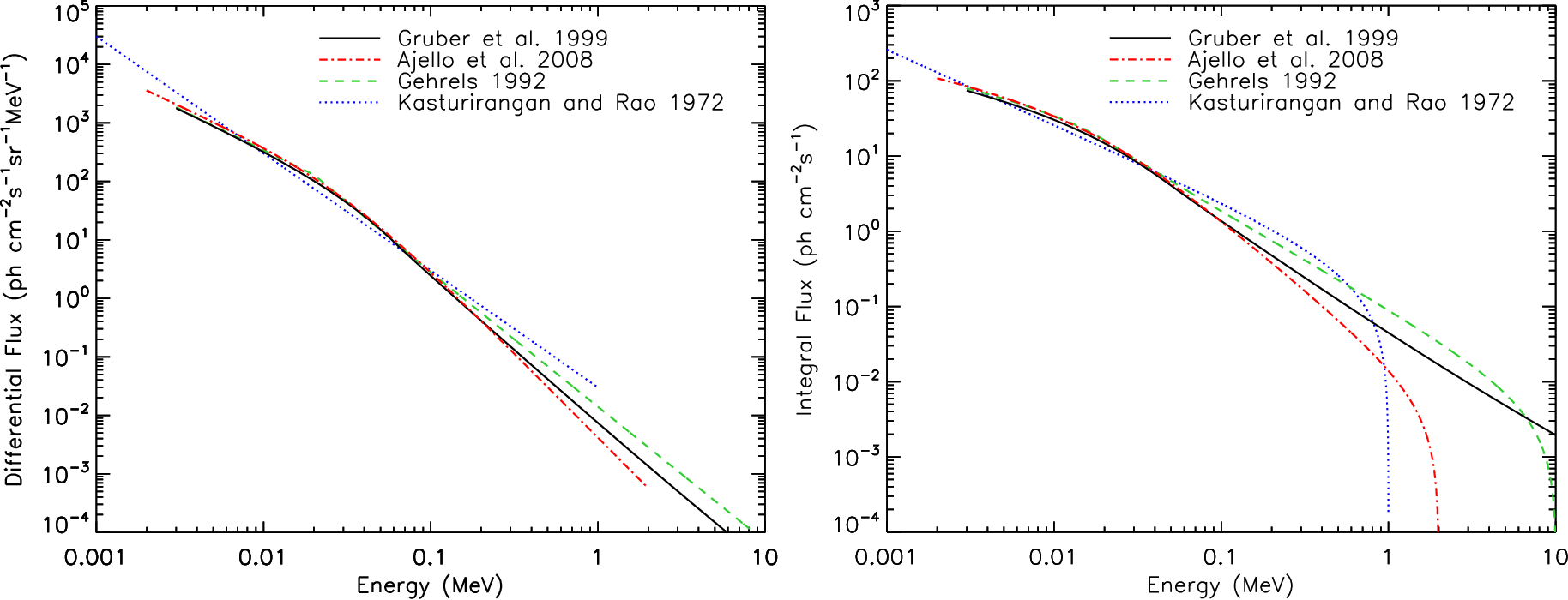
There are several empirical models used to describe the measured flux [74, 60, 105, 84, 69]. In our simulations we compare two models: the model introduced by Gruber et al. (1999) [105] and the one derived by Ajello et al. (2008) [84] (see Sec. 7).
The Gruber et al. (1999) model [105] fits the low-energy as well as the high-energy part of the CXB measurements obtained by HEAO-1 [106], CGRO/COMPTEL and CGRO/EGRET [107] instruments across a wide energy range spanning from 3 keV to 100 GeV. This empirical model is used as a standard in modeling of the CXB flux for planning space missions.
The differential photon flux in units of ph cm-2s-1sr-1keV-1 is:
for energies keV
| (3) |
and for energies keV it is
| (4) |
Ajello et al. (2008)[84] derived a CXB model which is in a good agreement with measurements from Swift/BAT[84], HEAO-1[105], INTEGRAL[82], BeppoSAX[83] instruments and other missions in the 2 keV – 2 MeV energy range. The differential photon flux in units of ph cm-2s-1sr-1keV-1 is:
| (5) |
where the parameters with 1 errors are , , and keV.
The CXB flux is omnidirectional and for 500 km altitude it irradiates a satellite from a solid angle of 8.64 sr (3.93 sr are occulted by the Earth). The CXB spectra for different models, including the two previously discussed, are shown in Figure 4. The integral flux, i.e. the integrated flux for energies above a given energy threshold, for the Gruber et al. (1999) model [105] and for keV is 30.3 ph cm-2s-1 whereas for the Ajello et al. (2008) model the integral flux at the same low-energy threshold is 33.7 ph cm-2s-1.
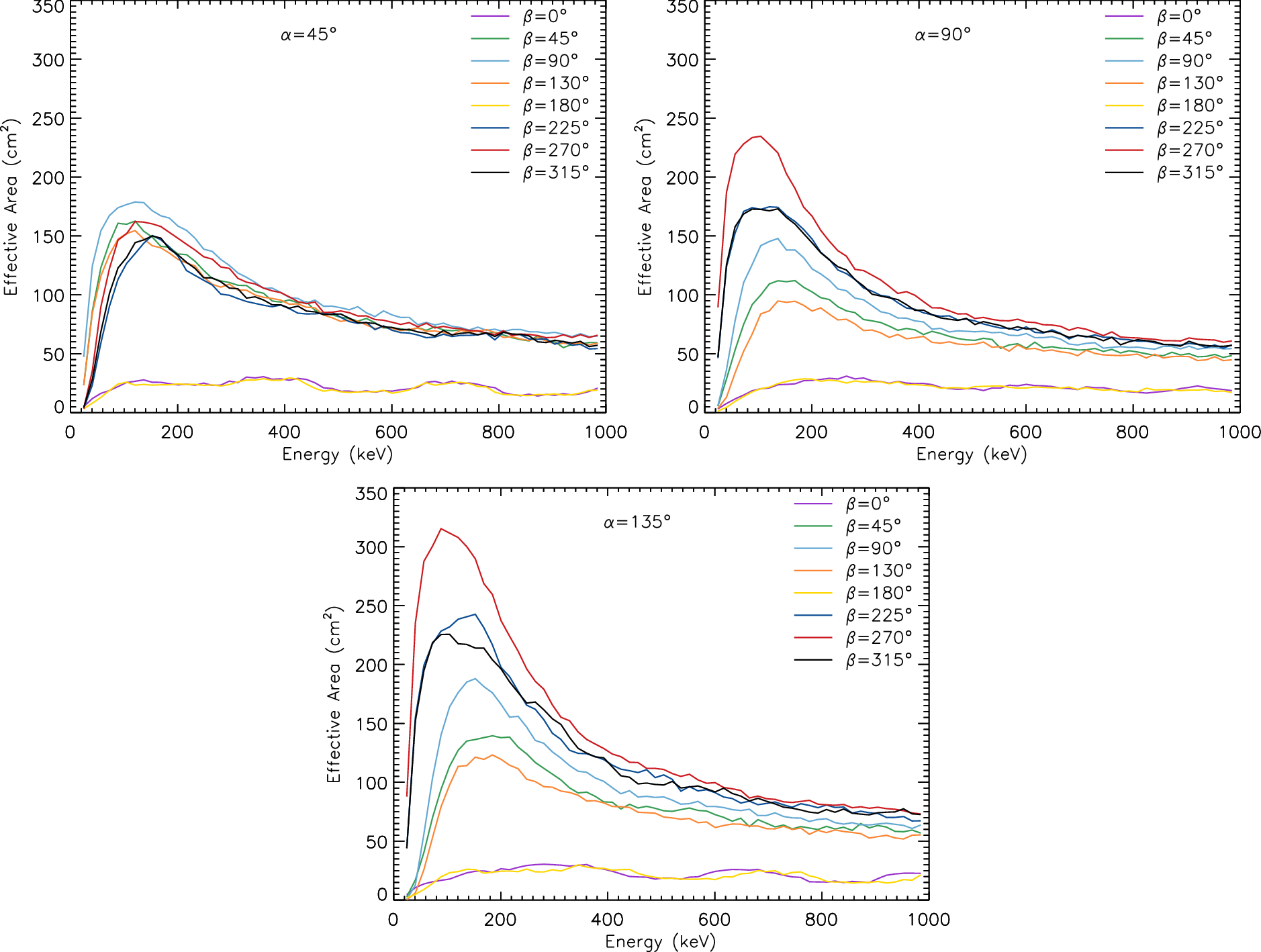
Concerning the CAMELOT CubeSats, the detectors are 5 mm thick CsI(Tl) scintillators (as described in Sec. 4) with effective area having maximum at keV (see Figure 18). The scintillator is relatively transparent to gamma-rays above 2 MeV. For example the effective area at 1 MeV is a factor of about 7 lower than at 100 keV. Although some gamma-rays can cause pair-production or Compton scatter in the material of the satellite and then lower-energy gamma-rays can reach the scintillator, the CXB flux above 2 MeV is much lower than at few tens of keV or at 100 keV. Therefore, the high-energy gamma-ray component (above few MeV) included in the Gruber et al. (1999) model [105] is not essential for the CAMELOT’s detectors.
Ajello et al. (2008)[84] discusses that the normalization of the Swift/BAT CXB spectrum at 30 keV (CXB peak) is % higher than the HEAO-1[105] measurement and consistent with the INTEGRAL[82] one. Also, the HEAO-1 measurement has 10 % precision at the CXB peak. Therefore, we use both CXB models to simulate the expected detected background by CAMELOT, however, for a more detailed analysis, e.g. detected count rate as a function of energy threshold, we choose a more conservative approach and use the Ajello et al. (2008) model which gives % higher integral flux in the energy range of keV, which is approximately the sensitivity range of CAMELOT’s detectors.
3.2 Galactic Emission
The Galactic gamma emission [108, 109] which consists of diffuse continuum [110] and resolved sources has been widely observed by many instruments, e.g. by SAS-2 [111, 112, 77, 113], OSO-3 [114], COS B [115, 113], INTEGRAL [116, 82, 117, 118, 87, 119, 120] satellites, COMPTEL, EGRET and OSSE instruments [121, 81, 122, 123, 124] aboard the CGRO satellite, Fermi/LAT [88, 125, 126, 127], RXTE/PCA [128] and Swift/BAT [129] instruments.
For our MC simulations (Sec. 7) we took the X-ray/gamma-ray fluxes of the inner Galactic region from Figures 10 and 11 as published in Ref. [87] in flux density representation. Ref. [87] summarizes measurements from RXTE/PCA[116], INTEGRAL/SPI[118], INTEGRAL/IBIS[116, 87], CGRO/COMPTEL[117] and CGRO/EGRET[117] instruments and show the fluxes renormalized to the central radian of the Milky Way defined by and .
The emission from the inner Galactic region irradiates a satellite from the solid angle of 0.542 sr. The differential and integral photon spectra are shown in Figure 5. The integral flux for energy keV is 0.2 ph cm-2s-1. However, it should be noted that the Galactic emission is not spatially uniform and has a brightness structure peaked at the Galactic center (see e.g. Ref. [115]). Figure 5 also shows measurements done by Fermi/LAT taken from Figure 4 of Ref. [125] for smaller region of and . We do not include these Fermi/LAT measurements in our MC simulations because the region of the inner Galaxy is not exactly the same as the one used for the other aforementioned data sets. This does not effect our results because the photon flux at these very high energies is very small.

3.3 Trapped Particles
The fluxes of the geomagnetically trapped electrons and protons inside the inner van Allen radiation belt [130] contribute to the overall detected instrumental background and they are especially important when a satellite at LEO passes the polar regions [131, 132] or the South Atlantic Anomaly (SAA). Details about the Earth’s radiation environment can be found in, for example, Ref. [133, 58, 134, 135, 64, 136, 137, 138, 139].
Several models describing the fluxes of the trapped particles around the Earth based on measurements from tens of space missions have been developed over last decades, e.g. the National Aeronautics and Space Administration’s (NASA) AE8 [140, 141] and AP8 [142, 141] models, European Space Agency’s (ESA) AE-8 update ESA-SEE1 [143] model, or model based on the measurements from Proton/Electron Telescope (PET) onboard the Solar, Anomalous, and Magnetospheric Particle Explorer (SAMPEX) satellite - the SAMPEX/PET PSB97 model [144].
In our on-board background simulations (Sec. 7) we employ the fluxes of trapped electrons and protons prescribed by the recent AE9 and AP9 models [145, 146, 147, 148] as they are implemented in ESA’s SPace ENVironment Information System (SPENVIS55 5 www.spenvis.oma.be). SPENVIS is an Internet interface to models of the space environment and its effects, developed by a consortium led by the Royal Belgian Institute for Space Aeronomy (BIRA-IASB). The AE9/AP9 models are based on 33 satellite data sets from 1976 to 2011 and they are provided by the U.S. Air Force Research Laboratory (AFRL) in their software package 66 6 https://www.vdl.afrl.af.mil/programs/ae9ap9.
The AE8/AP8 models available in SPENVIS or in the AFRL package do not compute fluxes lower than 1 particle cm-2s-1, whereas the AE9/AP9 models provide fluxes below 1 particle cm-2s-1. That is important for our purpose, because we want to estimate the detected background count rate in the regions outside SAA and polar regions. However, the current version of the AP9/AE9 model provided in SPENVIS is recommended for evaluation purposes only and there have been reported discrepancies between the AE8/AP8 and the AE9/AP9 models, e.g. see Ref. [149] and references therein.
Figure 6 shows orbit-averaged integral spectra of trapped electrons and protons averaged over 60 days of orbiting (including SAA passages) with sampling of 10 s obtained for different models by the AFRL package. It demonstrates that AE9/AP9 models gives much higher electron and proton fluxes compared to the AE8/AP8 models at low inclinations and low energies. Therefore the detected background count rate due to the trapped particles calculated by our simulation may overestimate the real level.

Figure 7 shows maps of integral fluxes (flux of particles with energy higher than ) of trapped electrons and protons for the AE9 and AP9 models with Monte Carlo (MC) mode, 100 runs and 50 % confidence level (CL) at 500 km altitude. The MC mode accounts for the uncertainty due to the random perturbations as well as the flux variations due to the space weather [145].

We calculated spectra of electrons and protons averaged along the trajectory of a satellite at altitude 500 km with inclination of and orbiting 30 days with flux sampling every 10 s. Only the regions with the integral flux particle cm-2s-1 were used ( keV for electrons and keV for protons). These conditions give a duty cycle, i.e. the fraction of time a satellite spends in a region with particle flux lower than a given flux threshold, of 80 %. If the orbital inclination is the duty cycle would be 76 %. Details about the duty cycle for different inclinations, altitudes at LEO, flux and energy thresholds for AE8, AP8, AE9 and AP9 models can be found in Ref. [150].
In this way we were able to obtain averaged spectra outside of SAA. The differential and integral fluxes are shown in Figure 8. The differential flux per solid angle has been calculated for simplicity assuming the radiation is illuminating a satellite isotropically from the solid angle of because, for example, in case of CAMELOT satellites the pointing strategy is not established yet. The trapped particles can collide with the detector from various directions and we are interested in a long-term average. Also, the assumption of the isotropy of the trapped particle flux is a simplification because of the well known “East-West” effect [151]. The integral flux for trapped electrons is 0.41 cm-2s-1 ( keV) and for trapped protons is 0.14 cm-2s-1 ( keV) as obtained from the model.

3.4 Primary Cosmic-Rays
The spectra of the primary particles of cosmic-rays (CRs) used in our simulations are described below. For the assumed 500 km altitude the fluxes irradiate the satellite from the solid angle of 8.64 sr. The origin of CRs is extraterrestrial consisting mainly of protons. Other components of CRs such as electrons, positrons, alpha particles and nuclei of heavier elements have been detected as well. Several experiments have been performed to study CRs, e.g. AMS [152, 153], BESS [154], CREAM [155], Fermi/LAT [156, 157], HESS [158], PAMELA [159].
We considered two models for the spectra of primary particles. The first one was the ISO-15390[160] model, which is the international standard for estimating the radiation impact of CRs on hardware in space and which describes the fluxes of primary protons, alpha particles, and nuclei of heavier elements.
The second model which we considered was described by Mizuno et al. (2004), see Ref. [63], and it was based on measurements done by BESS and AMS experiments (see also Ref. [66]). The flux of primary CRs in interstellar space can be modeled by a power law function:
| (6) |
where is the rigidity of the particle as a function of its kinetic energy or momentum and its charge . The flux constant and the exponent are determined by fitting of the following model to the measurements.
The flux of primary CRs for a given phase of the solar cycle and in a given position in the Earth’s magnetosphere according to the model described in Ref. [63] is:
| (7) |
where is the mass of the particle, is a solar modulation potential, is the altitude of the satellite’s orbit and is the geomagnetic latitude.
By applying an effective shift of energy of the primary particles due to the deceleration by the solar wind the first function in Eq. (7) gets form:
| (8) |
The second function accounts for the flux modulation due to the solar cycle and is given by:
| (9) |
where the solar modulation potential varies between GV for solar minimum and GV for solar maximum.
The third term is the geomagnetic cutoff function given by:
| (10) |
where for or particles, for or , and the cutoff rigidity is given by the Störmer equation [161]:
| (11) |
where is the Earth’s radius.
We want to estimate a long term average of the flux, therefore we assume that the flux has uniform angular distribution for the zenith angle and the flux is zero for , where the is the zenith angle of the Earth’s horizon and it is for the altitude of 500 km.
3.4.1 Primary Protons and Alpha Particles
For primary protons and alpha particles we compared the model ISO-15390 and the model Mizuno et al. (2004) described in Ref. [63].
For the ISO-15390 model we employed SPENVIS where we generated the orbit-averaged spectra for circular orbit with inclination , duration 30 days and sampling 60 s. The following parameters setting was applied: solar minimum activity (May 1996), magnetic shielding on, stormy and quite magnetosphere, Størmer with eccentric dipole method and magnetic field moment unchanged.
For the model described in Ref. [63] we used the following parameters: solar minimum cycle with the solar modulation potential GV, altitude 500 km, and two geomagnetic latitudes and (orbital inclination) + (tilt between the geomagnetic dipole axis and the Earth’s rotational axis).
For primary protons the values of particle m-2s-1sr-1MeV-1 and were adopted. For primary alpha particles the values of particle m-2s-1sr-1MeV-1 and were adopted.
Figure 9 and 10 show fluxes of primary protons and alpha particles, respectively, at 500 km altitude obtained by the ISO-15390 model for quiet and stormy magnetosphere and obtained by the Mizuno et al. (2004) model for fixed geomagnetic latitudes and . This model predicts the integral flux of primary protons of kinetic energies GeV being 0.11 cm-2s-1 (for ) or 0.29 cm-2s-1 (for ) and the integral flux of primary alpha particles of kinetic energies per nucleon GeV/n being 0.016 cm-2s-1 (for ) or 0.041 cm-2s-1 ().
For our Geant4 simulations of the expected on-board background by a CAMELOT satellite (Sec. 7) we use the ISO-15390 model with stormy magnetosphere, because it is the international standard for CR flux and because it was obtained for a fixed orbital inclination of meaning crossing the range of geomagnetic latitudes between and 77 7 https://spawx.nwra.com/spawx/maps/maplats.html, [162]. It predicts the integral flux of primary protons of kinetic energies GeV being 0.095 cm-2s-1 (for quite magnetosphere) or 0.099 cm-2s-1 (for stormy magnetosphere) and the integral flux of primary alpha particles of kinetic energies per nucleon GeV/n being 0.017 cm-2s-1 (for quite magnetosphere) or 0.018 cm-2s-1 (for stormy magnetosphere).


3.4.2 Primary Electrons and Positrons
For the spectra of the primary e- and e+ we used the model described by Mizuno et al. (2004) [63] with references to the flux measurements by [163, 164]. The measurements of the ratio of positrons and electrons e+/(e-+e+) are given by [165, 153].
We adopt the model of the primary interstellar particles Eq. (6) with following parameters: particle m-2s-1sr-1MeV-1 and for electrons and particle m-2s-1sr-1MeV-1 with the same exponent for positrons.
Same as for the primary protons and alpha particles we used the following conditions of the solar cycle and the orbit: solar minimum with the modulation potential GV, altitude 500 km, and two geomagnetic latitudes and . Figure 11 and 12 show the fluxes of the primary electrons and positrons.
For our simulations of the expected detected background (Sec. 7) we use the spectrum for . We also assume that the angular distribution of the flux is incoming uniformly from the solid angle unocculted by the Earth. Then the integral flux ( GeV) for e- is cm-2s-1 and for e+ it is cm-2s-1.


3.5 Secondary Particles and Radiation
Secondary (albedo) particles and radiation are created by interaction of primary CRs with the Earth’s atmosphere [58, 64].
3.5.1 Secondary Protons
For secondary p+ and for energy above 100 MeV we use the model [63] based on the measurements done by the Alpha Magnetic Spectrometer (AMS) [152] from 380 km altitude for the geomagnetic latitude . For energy below 100 MeV we use the fit to MITA/NINA-2 data [166] from 450 km altitude and for , where L-shell is the McIlwain L-parameter [167]. For details see the LAT Technical Note LAT-TD-08316-01 [72] of the Fermi satellite [168]. There is only small dependence of the flux on altitude [166, 169] therefore it can be used as an approximation to the flux at altitude of 500 km.
The differential flux in units of particle m-2s-1sr-1MeV-1 is modeled as:
| (12) |
where MeV is break energy. Figure 13 shows the modeled flux together with the measurements.
The same model is used for the upward and downward component of the flux and it is assumed that secondary protons irradiate the satellite from the solid angle of sr without zenith-angle dependence of the flux. The integral flux ( MeV) is 0.037 cm-2s-1.

3.5.2 Secondary Electrons and Positrons
For secondary e- and e+ and for energy above 100 MeV we use the model [63] based on the measurements done by AMS [152] from 380 km altitude for the geomagnetic latitude . For energy below 100 MeV we use the fit to Mir/MARIA-2 data [170, 171] from 400 km altitude and for . For details see the LAT Technical Note LAT-TD-08316-01 [72].
For secondary e- the differential flux in units of particle m-2s-1sr-1MeV-1 is modeled as:
| (13) |
where the break energy MeV. Figure 14 shows the modeled flux together with the measurements.

For secondary e+ the differential flux in units of particle m-2s-1sr-1MeV-1 is modeled as:
| (14) |
where the break energy MeV. Figure 15 shows the modeled flux together with the measurements.

The same model is used for the upward and downward component of the flux and it is assumed that secondary e- and e+ irradiate the satellite from the solid angle of sr without zenith-angle dependence of the flux. The integral flux ( MeV) is 0.18 cm-2s-1 for e- and 0.23 cm-2s-1 for e+.
3.5.3 Albedo X-rays/-rays
The secondary (albedo) X-ray and -ray flux is due to interaction of primary CRs with the Earth’s atmosphere. It is produced by decay of pions (mainly above 50 MeV), by bremsstrahlung from primary and secondary electrons (mainly below 50 MeV), and also by the reflection of CXB and it has been measured by several satellites and balloon experiments [75, 172, 76, 78, 173, 174, 60, 175, 61, 63, 176, 64, 82, 177, 87, 69]. The intensity depends on the geomagnetic latitude [178].
We utilize a model reported by Ajello et al. (2008) [84] based on the Swift/BAT measurements from keV to keV for altitude of km and inclination of and which is compatible with measurements from BeppoSAX[83] ( km and ) and after some corrections with measurements by the polar-orbiting satellite 1972-076B [178] ( km). MC simulations show that this model is a very good approximation of the Earth albedo X-ray emission up to 300 keV [179, 84].
We assume the Ajello et al. (2008) model [84] in the energy range of keV and hence the differential photon flux given by Eq. (5), where the model parameters and their 90 % CL errors are =-5 (fixed), =1.72, =33.7 keV and .
For higher energies we assume a model reported by Mizuno et al. (2004) [63] based on measurements by 1972-076B and Kosmos 461 satellites [178, 173] and by balloon flights [172, 174]. Particularly, we consider only energies MeV where we assume the differential photon flux in units of ph cm-2s-1sr-1keV-1 to be a simple power law function:
| (15) |
where we normalized the Mizuno et al. (2004) model [63], their Eq. (21), in order to obtain the same differential flux at 300 keV as predicted by the Ajello et al. (2008) model [84]. The spectrum is shown in Figure 16. According to MC simulations [179] there is only a small dependence of the albedo X-ray flux ( keV) on the solar cycle and geomagnetic latitude below for an instrument at LEO with large FOV which covers the whole terrestrial disc.

A zenith angle dependence of the albedo -ray flux has been measured in the MeV region [76, 75, 63]. See also Ref. [114, 172, 178, 174, 180, 175, 61, 176, 177] and references therein for the zenith angle dependence of the albedo -ray flux at other energies. In the energy range keV, covered by the Ajello et al. (2008) model, the MC simulations [179] suggest that there is no zenith angle dependence. However, for the higher-energy part MeV one can expect a zenith angle dependence of the flux. In case of CAMELOT satellites, they will have detectors with all-sky FOV which can be illuminated from various directions and we are interested in a long term average flux, therefore, for simplicity, we do not assume any zenith angle dependence in our Geant4 simulations involving a CAMELOT satellite mass model.
At an altitude of 500 km the photons would irradiate the satellite from a solid angle of 3.93 sr. The integral flux ( keV) is 3.1 ph cm-2s-1.
3.5.4 Albedo Neutrons
The albedo neutrons are produced in hadronic showers created by CRs interacting with the Earth’s atmosphere and they can reach a satellite at LEO [69]. For the albedo neutrons we use the predictions of the QinetiQ Atmospheric Radiation Model (QARM), based on MC radiation transport code, as reported in the ESA document ECSS-E-ST-10-04C [71]. The model has been validated against several measurements [181, 182, 183, 184] and is also consistent with other MC simulations[59, 65]. For other models and measurements see Ref. [185, 61, 186, 69] and references therein.
Figure 17 shows the fluxes of secondary neutrons for the cutoff rigidity GV and GV for solar minimum. The fluxes were scaled from the altitude of 100 km to 500 km as described in the ECSS-E-ST-10-04C document.
In our simulations of the expected detected background (Sec. 7) we use the spectrum for the solar minimum and for the cutoff rigidity GV which corresponds to the geomagnetic latitude following from the Störmer equation Eq. (11) or latitude between and , see Figure 7 of Ref. [161].
The integral flux is 0.61 cm-2s-1 for eV, for GV, altitude of 500 km and assuming that all neutrons are coming from the solid angle of 3.93 sr which corresponds to the angular size of the Earth observed from that altitude.

4 The CAMELOT CubeSats
We study in particular the expected on-board background for the proposed CAMELOT mission, expected to be launched to LEO with the main objective of all-sky monitoring and timing-based localization of GRBs. The at least nine satellites are considered to be placed on orbits with altitude of km with inclination of or at Sun-synchronous orbits of inclination [2]. One of the options for the CAMELOT satellite platform is the one being developed by C3S LLC in Budapest, therefore we apply its mass model in our Geant4 simulations.
4.1 The Detector System
The constellation of at least nine 3U CubeSats is proposed to be equipped with large and thin CsI(Tl) scintillators, of size mm3 each, read out by Hamamatsu Multi-Pixel Photon Counters (MPPC). There would most likely be four scintillators on each satellite with two scintillators placed on two neighbouring sides of the satellite. The scintillators will be wrapped in the enhanced specular reflector (ESR) foil and enclosed in a support structure made either from aluminium or carbon fiber-reinforced plastic (CFRP). For details about the detector system see Ref. [187]. The effective area of four detectors on board one CAMELOT satellite as a function of energy and for different directions, obtained from Geant4 simulations, is shown in Figure 18.
In order to understand and characterize the behaviour of the large-area CsI(Tl) scintillator detector and the MPPC readout, an experimental setup was built in Hiroshima, Japan. The experimental setup provided vital information for the simulation, mostly for the position dependence of the scintillator effective light yield. Different sources were used in the tests, mostly an 241Am source [188].
5 Validation of Geant4 Simulation and Calibration of Detector’s Optical Parameters
A dedicated set of measurements were carried out with 241Am source with an activity of 471 kBq which was collimated to irradiate different positions on the scintillator. The experiments were carried out with a single MPPC very similarly to the measurements presented in Ref. [188]. The collimation was achieved with two lead sheets each containing holes in nine positions. In order to obtain the optical parameters of the scintillators as precisely as possible, the effect of reflectivity and absorption length on photon light yield was maximized by utilizing one MPPC in the middle of the shorter side of the scintillator. Spectra were recorded in nine cases by moving the 241Am source in the nine positions where holes were present. Figure 19 shows the simulation of the experimental set-up.
The measured and simulated spectra for the irradiation point closest to the MPPC and in the farthest corner are compared in Figure 20. The same number of X-rays were simulated, which were emitted in 2 minutes of data acquisition for each spectrum. The difference between these spectra is the largest of all. The main reason for this is the difference in the mean path of optical photons, which is the shortest when the source is in front of the MPPC and the largest when the source is placed in the corner.
 |
Two distinct peaks are visible in the measured and simulated spectra (Figure 20). The peak with the higher energy corresponds to the 241Am peak at 59.5 keV. The lower-energy one is the Kα X-ray fluoresence peak of the Cesium in the scintillator [188]. The results of the Geant4 simulation were smeared by a Gaussian function with a standard deviation of 5 channels for the closest point of irradiation and 15 channels for the farthest to match them with the measured ones. The histogram of the number of photons detected in the simulation were scaled up by 1.35 and 1.39 respectively to match them with the measurements. This way assuming a linear detector response, all amplification factors were treated together. The fact that the scaling factor is almost the same for all parts of the scintillator translates to a good light collection efficiency. The main aim of the measurements was to determine the number of detected optical photons for an energy deposition of 1 keV in the scintillator (on average). For the measurements taken at the farthest position from the MPPC the 59.5 keV 241Am peak was at ADC channel 180. The number of detected photons in the simulations had to be scaled up by roughly 1.37 to match the measurements. For the measurements taken at the closest point to the MPPC the same scaling parameter was used. For the farthest position from the MPPC this implicates that an energy deposition of 1 keV yields 4.11 detected optical photons on average.

The light yield in the simulation for the scintillator was fixed at 54 photons/keV, which is the yield for CsI(Tl) scintillators produced by Saint-Gobain88 8 https://www.crystals.saint-gobain.com/products/crystal-scintillation which is similar to our scintillator produced by AMCRYS99 9 http://www.amcrys.com. The absorption length and the reflectivity of the surface of the scintillator was varied until the simulation agreed with the measurements for the two extreme spectra, the one in front of the MPPC and the one in the farthest corner. The best fitting reflectivity was 99.99 % and the absorption length determined from the fit was 60 cm. These values were used in the later simulations.
In this way of calibration the energy resolution and noise of the electronics are taken into account in the simulations. Although pileup is not included but during operation we do not expect such high count rates from regular sources where it could be relevant.
6 Description of Geant4 Simulations
A Geant4 MC based simulation was developed in order to understand how the CAMELOT CubeSat constellation would detect -rays originating from short GRBs, long GRBs and TGFs. This required dedicated simulations of each background component as well as response to the -ray sources and calculation of the signal-to-noise ratio. The repository containing the simulation source code and analysis code are shared on GitHub (with a GNU General Public License). 1010 10 https://github.com/ggalgoczi/szimulacio/tree/master/Bck_4.10.6,1111 11 https://github.com/ggalgoczi/szimulacio/tree/master/GRB.
As the first step, the experimental setup that was used to calibrate the optical parameters of the CsI(Tl) scintillator – the -ray detector of the satellite – that with its casing was implemented in Geant4. Details are in Sec. 5. Afterwards the complex CAD model (Sec. 6.2) of the satellite – consisting of 7 modules, each with a given average material composition – was imported to Geant4 with CADMESH [189]. Four scintillators, each read out by 8 MPPCs were placed on two sides of the satellite.
In order to keep computation time at a reasonable level, the simulation of each primary particle is stopped if the number of detected optical photons reaches 10 000. Heavy ions can create several hundred thousands of scintillation photons. This limitation made it possible to run the codes on personal computers with a few cores. The signal of the 8 MPPCs is planned to be grouped into two groups of 4 MPPCs. In the following simulations the signal of all 32 MPPCs belonging to the four scintillators is summed up. This way we give a conservative signal-to-noise ratio (SNR) estimation since a more sophisticated trigger algorithm will decrease the chance of the background to exceed the threshold in each channel. The energy deposition is calculated from the number of detected optical photons. As described in Sec. 5, 1 keV energy deposition corresponds to 4.11 optical photons detected in the simulation. This corresponds to an overall photon detection efficiency of 7% which is expected given the large size of the scintillator, the small sensitive area of MPPCs and the quantum efficiency of the MPPCs which depends on the scintillation light wavelength.
6.1 Directional and Positional Distribution of Primary Particles
The simulations presented in this paper can be split into two main groups based on whether we are simulating the source of the background or an astrophysical source. The latter are the target objects: sGRBs, lGRBs and TGFs, which can be considered as point sources very far away, therefore photons coming from these sources are treated in the simulations as parallel.
The other main group is the background (eg. CXB, albedo particles, trapped electrons). The background particles and -rays mainly hit the satellite from large solid angles or isotropically. The pointing strategy of the CAMELOT satellites is not established yet and the detector has all-sky FOV. We are interested in the estimation of a long-term average background at the regions of low geomagnetic latitude and outside SAA as mentioned in Sec. 3. Therefore, as an approximation, we assume that all components of the background flux of particles and -rays irradiate the satellite isotropically.
In order to realize this in the simulations the background particles were placed randomly on a sphere with a radius around the model of the satellite. To maintain isotropy their direction was also randomly chosen. To boost up the simulation a source biasing was used [190] to limit the number of primary particles simulated to the ones which would hit the satellite. Due to the biasing, the number of detections in the simulation had to be normalized to determine the detection rate we would actually have.
The expected detection rate for CAMELOT in space can be calculated as follows [190]:
| (16) |
where is the factor which takes into account the solid angle of the type of the background. For instance albedo particles originate only from the atmosphere beneath the satellite. This corresponds to 3.95 sr for our orbit. is the radius of the sphere upon which the primary particles are distributed. This radius needs to be much larger than the size of the target object to maintain isotropy. stands for the angle that is formed by the initial direction of the simulated primary particle and the vector pointing to the center of the satellite from the origin of the simulated primary particle. By limiting we are able to simulate only those particles which would hit the satellite. In our case m. and are the upper and lower bounds for the chosen interval of the emission angle in the simulation. In our case and . is the flux in units of cm-2s-1sr-1. is the number of detections in the given simulation. is the number of primary particles shot in the simulation. The factor cm2. Table 2 summarizes the values of and the normalization factor for the background models described in Sec. 3.
| CXB and | Galactic | Trapped and charged | Albedo | |
| primary CR | secondary particles | and n0 | ||
| (sr) | 8.64 | 0.542 | 3.93 | |
| (cm2sr) |
6.2 Satellite’s Mass Model
In order to include all parts of the satellite including even the smallest volumes, the detailed CAD model of the satellite was read into Geant4 directly with CADMESH [189] that utilizes TETGEN [191] and ASSIMP1212 12 http://www.assimp.org software libraries to directly read in STL files into Geant4. The satellite consists of seven modules including the structure of the satellite, the communications module, the payload etc. The only volume that was not included were the antennas. The material of each of the volumes was averaged (as described in Table 7. and Table 8.). The complete list of alloys used in each volume are listed in Sec. 10 together with their composition. Figure 21 shows the mass model of the CAMELOT satellite. Figure 30 in the Appendix presents the individual volumes of the satellite.
 |
7 Results of Geant4 Simulations
7.1 Response to Each External Background Components
In this section the simulation results of the satellite response to each of 14 external background components is presented. The results are for one CAMELOT satellite. The count rate is summed for all detectors. By far the most relevant background is CXB. Therefore we chose to simulate two different CXB models introduced by Gruber et al. (1999) [105] and Ajello et al. (2008) [84] described in Sec. 3.1. The input energy spectra of each background component used for the simulations are described in the corresponding subsection of section 3. The model of the satellite was irradiated isotropically as shown in Figure 22.
 |
Four possible aluminium detector support structure (shortly detector casing or just casing) thicknesses were investigated. The same material and thickness is on all sides of the detector housing, including the back side. In order to give an idea of the contribution of each component a realistic 20 keV low-energy threshold was chosen. The five components which contribute the most to the background for the casing thickness of 0.5 mm thick Al with this low-energy threshold are: CXB ( counts per second (cps)), albedo ( cps), primary CR protons (27 cps), albedo protons (45 cps) and albedo positrons (28 cps). Tables 3 and 4 summarize the background detection rate predicted by the simulation.
| Thickness | CXB | CXB | CR | CR | Galactic | Trapped | CR | CR | Trapped |
|---|---|---|---|---|---|---|---|---|---|
| (mm) | A08 | G99 | p+ | p+ | e- | e+ | e- | ||
| 0.5 | 1150 | 996 | 51 | 28 | 5.12 | 1.15 | 0.74 | 0.057 | 0.17 |
| 1.0 | 1020 | 893 | 49 | 29 | 3.98 | 0.947 | 0.76 | 0.057 | 0.073 |
| 1.5 | 890 | 770 | 51 | 29 | 4.04 | 0.820 | 0.76 | 0.060 | 0.072 |
| 2.0 | 858 | 707 | 51 | 29 | 3.50 | 0.827 | 0.75 | 0.059 | 0.066 |
The background detection rate is in counts per second, assumes a low-energy threshold of 20 keV, and is simulated for different thicknesses of the aluminium support structure of the detector. Two spectral models described by Gruber et al. (1999) [105] and by Ajello et al. (2008) [84] (denoted as G99 and A08) were simulated for the CXB. For the primary CR p+ and particles we used the ISO-15390 model with stormy magnetosphere and inclination of . For primary CR e- and e+ we used the model described by Mizuno et al. (2004) [63] for solar minimum, . For trapped e- and p+ we used the AE9 and AP9 models, respectively, for inclination of , MC mode and derived from the 50 % CL of the fluxes. Altitude of 500 km was chosen.
| Thickness (mm) | Albedo | Secondary e+ | Secondary e- | Secondary p+ | Albedo n0 |
|---|---|---|---|---|---|
| 0.5 | 208 | 28.2 | 6.32 | 45.5 | 23.8 |
| 1.0 | 205 | 27.1 | 8.00 | 43.7 | 22.3 |
| 1.5 | 192 | 27.4 | 7.95 | 42.5 | 22.3 |
| 2.0 | 191 | 28.2 | 7.86 | 43.4 | 21.4 |
The detection rate is in counts per second, assumes a low-energy threshold of 20 keV and is simulated for different thicknesses of the aluminium support structure of the detector. For secondary neutrons the spectrum for the solar minimum and for the cutoff rigidity GV was used.
By summing up the contribution of each background component we derived a total background rate of 1550 cps for 0.5 mm, 1400 cps for 1 mm, 1270 cps for 1.5 mm and 1100 cps for 2 mm of the casing thickness assuming a low-energy threshold of 20 keV. From the two CXB models simulated, the Ajello et al. (2008) model was chosen since it gives a more conservative estimate. The Ajello et al. (2008) and Gruber et al. (1999) models have integral fluxes of 33.7 ph cm-2s-1 and 30.3 ph cm-2s-1 for keV and give background rates of 1020 cps and 893 cps for 1 mm thick Al detector casing, respectively.
The low-energy threshold onboard the CAMELOT satellites is planned to be a tunable parameter and changeable upon a ground command. Laboratory experiments show that low-energy threshold for our detectors is around keV. In Figure 23 the detection rate is shown for different casing thicknesses and low energy thresholds. The low energy part of the background spectrum is dominated by CXB X-rays which are stopped by thicker detector casing. The higher energy part is dominated mostly by hadrons and albedo gamma rays (hard spectrum) which can easily cross aluminium and deposit high energies in the scintillator.
 |
7.2 Simulation of a Typical Short GRB from Different Directions
In order to quantify if CAMELOT is capable of detecting X-ray sources we need to investigate the X-ray absorption by the satellite structures themselves. The four scintillators are placed on two sides of the satellite. Therefore the X-rays from half of the objects need to cross a certain part of the satellite before arriving to the detectors.
 |
To quantify the X-ray absorption of the satellite and to determine the count rate expected from sGRBs, different source directions were simulated. First, the satellite was rotated around its major axis by 10∘ 35 times to cover all directions around this axis. Afterwards the same was repeated for the minor axis of the satellite. A 1024 ms peak spectrum of a typical sGRB was used in the simulation. Details of typical sGRB spectra are described in subsection 2.1.
7.2.1 Rotating Around Major Axis for Short GRB
The satellite was rotated around its major axis (Z in Figure 24) by between each simulation. The simulated primary X-rays originated from the direction of the X axis. case corresponds to the scenario when X-rays arrive perpendicular to the surface of two of the scintillators. The count rate is the highest for when the angle between the direction of the photons and the surface normal of both detectors is . The combined projected area of the four scintillators is the largest in this scenario. The least favored direction is (see Figure 25).
 |
In Figure 26 the spectra of two directions are shown. As expected for the least optimal direction () the low energy part of the spectrum is suppressed. These are the X-ray photons which are not able to cross the material of the satellite.
 |
Different low-energy thresholds are possible to be set. Therefore, it is important to understand how the count rate of X-rays from sGRBs would change by varying the low-energy threshold. In Figure 27 the count rate for the most and least optimal direction is shown depending on the low-energy threshold. Up to about 100 keV the count rate does not decrease significantly. Also it is important to notice that the direction of the source is much more important than the thickness of the detector casing.
 |
7.2.2 Rotating Around Minor Axis for Short GRBs
The same procedure as described in subsection 7.2.1 was followed for investigating sGRB (for 1024 ms peak spectrum) directions around the minor axis (X in Figure 24). X-ray were simulated as a parallel beam coming from the Z direction. In Figure 28 the count rate for each direction is shown. is the least optimal. It corresponds to the case when all scintillators are seen from their edge. In this case the cross-section of the four scintillators combined is 7.5 cm2, which is about 3 % of the area in the most optimal direction during rotation around the minor axis.
 |
Since the background for the casing thickness of 2 mm is 1100 cps, a count rate of 165 cps is required from a sGRB to be observed with a significance of 5 . Therefore from the directions investigated with the rotation of the minor axis the interval between and is suitable for the detection of sGRBs.
7.3 Signal-to-Noise Ratio of X-ray/-ray Transients
For the detection of astrophysical objects, the final figure of merit is the SNR. It is important to mention that for the localization accuracy not only the SNR but also the number of detected photons is important for the cross-correlation of light curves. Electronic noise was neglected in the following calculations as the planned low-energy threshold set for detection is higher than the amplitude of the electronic noise.
Detection low-energy threshold can be set onboard the satellite. Therefore SNR was quantified for each astrophysical object in the function of low-energy threshold. The following equation was used to determine SNR:
| (17) |
where is the detected count rate spectrum of the signal, stands for the detected count rate background spectrum, is the low-energy threshold, is the high-energy threshold and is the exposure time. In our simulations we did not put boundary on the high-energy threshold, but the triggering algorithm onboard CAMELOT satellites will have capability to set both the low- and the high-energy thresholds.
The main aim of the CAMELOT mission is the detection and localization of sGRBs. Therefore it is important to understand with what significance could CAMELOT satellites detect these objects. Among the direction, when the satellite was rotated around its major axis SNR is the highest when the angle between X-rays from a GRB and the surface normal of both detectors is . We have the lowest SNR for the angle of (see Figure 25).
 |
When the simulated typical sGRB (for 1024 ms peak spectrum) is in the most optimal direction an SNR of can be achieved. SNR stays above 10 within the low-energy detection threshold range from up to 100 keV. The thickness of the aluminium detector casing affects SNR mostly for low values of the low-energy detection thresholds, since the main background component, CXB has a rather soft spectrum. For the least optimal direction among the directions investigated an SNR of 6 can be achieved. This characteristic is shown in Figure 29. The other directions, when the satellite was rotated around its minor axis (Figure. 28), are less favored. In these cases the cross section of the detectors are significantly lower.
Tables 5 and 6 summarize the simulated detection count rate induced by the X-ray/-ray transient sources and the expected SNR. For GRBs four different exposure times were used: 64, 256 and 1024 ms for sGRBs and 4096 ms for lGRBs. It should be noted that long triggering timescales of the order of several seconds or tens of seconds are readily affected by the time variation of background due to geomagnetic latitude (cutoff rigidity) change during the orbit and the activation background varying with time since SAA passages. The SNR calculated for such long integration time is effected by the background systematics. Varying background can cause false triggers and detectors with larger effective area are more vulnerable unless a sophisticated background modeling is part of the trigger algorithm.
Different missions has employed different triggering timescales. BeppoSAX/GRBM used adjustable timescale in the range from 7.8125 ms to 4 s in 10 steps [192]. CGRO/BATSE used time windows of 64 ms, 256 ms and 1024 ms [193]. Suzaku/WAM used triggering timescales of 1/4 s and 1 s [21]. HETE-2/WXM and FREGATE used timescales from 80 ms up to 10.5 s or longer, but they modeled background to remove trends which can cause false triggers [194]. Swift/BAT uses two types of rate triggers: i) “short” rate triggers with timescales 4, 8, 16, 32 and 64 ms which are traditional triggers employing single background period of fixed duration; ii) “long” rate triggers with timescales from 64 ms to 64 s which fit multiple background intervals to remove trends as pioneered by HETE-II [195]. Fermi/GBM uses triggering timescales of 16, 32, 64, 128, 256, 512, 1024, 2048, 4096 and 8192 ms [26]. In case of AGILE/MCAL, transients are searched using time windows of duration of sub-millisecond, 1, 16, 64 , 256, 1024 and 8192 ms [196, 197].
From Table 6 it is also seen that in contrary to one’s expectation, TGF SNR increases with thicker detector casing. The reason for this is the hardness of TGF spectrum. The median energy of X-ray photons originating in TGFs is 2 MeV. These have a few per cent chance to interact with the scintillator material. The thicker detector casing provides more material in which these energetic photons can interact and produce secondary particles. Therefore thicker casing yields in higher SNR. This study is important in order to understand sensitivity of different trigger time window durations necessary for designing efficient GRB trigger algorithm.
| Al | sGRB peak spectrum | lGRB peak spectrum | lGRB | TGF | SGR | ||||
|---|---|---|---|---|---|---|---|---|---|
| (mm) | 64 ms | 256 ms | 1024 ms | 64 ms | 256 ms | 1024 ms | fln. sp. | ||
| 0.5 | 1440 | 910 | 385 | 1190 | 924 | 758 | 326 | 34600 | 16200 |
| 1.0 | 1390 | 911 | 367 | 1139 | 908 | 715 | 309 | 38900 | 14000 |
| 1.5 | 1300 | 890 | 367 | 1110 | 840 | 674 | 292 | 37600 | 11900 |
| 2.0 | 1320 | 839 | 355 | 1058 | 815 | 662 | 277 | 38600 | 10500 |
The detection rate is in counts per second, assumes a low-energy threshold of 20 keV and is simulated for different thicknesses of the aluminium support structure of the detector. For short and long GRBs the 64 ms, 256 ms and 1024 ms peak spectra were used. For long GRB also the fluence spectrum (fln. sp.) was used.
| Al | sGRB peak spectrum | lGRB peak spectrum | lGRB fln. sp. | TGF | SGR | ||||
|---|---|---|---|---|---|---|---|---|---|
| (mm) | 64 ms | 256 ms | 1024 ms | 64 ms | 256 ms | 1024 ms | 4096 ms | 0.1 ms | 0.2 s |
| 0.5 | 9.27 | 11.7 | 9.91 | 7.66 | 11.9 | 19.5 | 16.8 | 8.79 | 185 |
| 1.0 | 9.35 | 12.3 | 9.87 | 7.66 | 12.2 | 19.2 | 16.7 | 10.3 | 167 |
| 1.5 | 9.23 | 12.6 | 10.4 | 7.89 | 11.9 | 19.2 | 16.6 | 10.6 | 149 |
| 2.0 | 10.1 | 12.8 | 10.8 | 8.08 | 12.5 | 20.2 | 16.0 | 11.6 | 142 |
The detection SNR has been calculated for different thicknesses of the aluminium support structure of the detector. The assumed background count rate is the sum of all components as described in Ref. 7.1. For the GRB peak spectra were used the exposure time 64 ms, 256 ms and 1024 ms. For the fluence spectrum (fln. sp.) of long GRB we used ms. For TGF we assume exposure time ms and for SGR s. For this TGF spectrum the SNR is only a theoretical value following from the formula. For example, for 1 mm thicknesses of the Al detector casing the expected detected number of counts within 0.1 ms from is 3.9 cnt, whereas the expected number of background counts is below 1 cnt (only 0.14 cnt).
8 Discussion
The background count rates obtained in our MC simulations were derived from models of fluxes of gamma-rays and particles averaged over various latitudes, depending on the particular flux component, below and outside SAA. The reason is that we aim to obtain an expected “mean” background rate in parts of orbit which are suitable for gamma-ray transient scientific data collection. However, in reality, the background rate will have time variation due to geomagnetic latitude (cutoff rigidity) change within the orbit and due to the activation background varying with time since SAA passages.
The foreseen orbital inclination of the CAMELOT satellites is above and option of polar orbits is also likely. Therefore significant background variation is expected as well. We investigated background count rates measured by Fermi/GBM, RHESSI[198] and Lomonosov/BDRG[131] gamma-ray instruments throughout their orbits to learn what background variations are expected. In case of Fermi/GBM (altitude 560 km and inclination 26∘) the background rate outside SAA for one NaI detector module in keV range varied throughout the orbit between cps and cps, i.e. change (about two months after the launch), see also Ref. [199]. In case of the RHESSI spectrometer (altitude 500 km and inclination 38∘) the background rate outside SAA for one rear detector segment in keV range varied throughout the orbit between cps and cps, .i.e. change (about three years after the launch) 1313 13 http://sprg.ssl.berkeley.edu/~tohban/browser/. For a detector on a polar orbit the background rate can increase dramatically more when passing the polar regions of trapped particles in the van Allen radiation belt. The Lomonosov/BDRG (altitude 550 km and inclination 98∘) measurements show that the rate outside SAA, in keV range increases inside the polar regions compared to the rates near equator (about 5 months after the launch), see also Ref. [131]. Therefore outside SAA and polar trapped particle regions the background count rate variation of at least the value near the equator for detectors on board the CAMELOT satellites are also foreseen. Inside the polar regions the rate increase can be much higher.
Since CubeSats which are not on equatorial orbit (currently most of them) are subject to high proton flux upon SAA passages, these protons have enough energy to activate the material of the satellite [69]. Short term activation is important as decaying isotopes can cause a strongly time-variable background for a few minutes after the end of SAA passes. Long term activation can increase the background significantly in a matter of months. [200] To quantify the effects of proton induced activation, we plan to conduct simulations in the near future. Emission lines of radioactive isotopes could also be used for energy calibration. As an example for our scintillators 123I will be created which emit -rays with an energy of 159 keV [201].
In order to discuss how our estimated background rates of CAMELOT detectors scale to the observations of Fermi/GBM, AGILE/MCAL and Suzaku/WAM we consider the surface area of the scintillators of these instruments and assume that these surface areas can be used as rough scaling factors. For CAMELOT (CsI): scintillators giving the area of cm2. For Fermi/GBM (NaI): giving the area of cm2 for one detector module (the effective area around 0.4 MeV is cm2) [202]. For AGILE/MCAL (CsI): detectors giving the area of cm2 (the effective area at MeV is cm2) [54]. For Suzaku/WAM (BGO) the area is cm2 [21].
The estimated background rates of CAMELOT detectors for 0.5 mm Al support structure are , and kHz respectively for keV, keV and keV (see Fig. 23). The observed background rates of one detector module of Fermi/GBM ( months after the launch, altitude km and inclination ) are kHz and kHz for keV and keV, respectively. For AGILE/MCAL ( km and ) the rate is kHz for keV. In case of Suzaku/WAM ( km and ) the rate is kHz for keV.
If we use the surface area of scintillators as a scaling factor than the background rate scaling between Fermi/GBM and Suzaku/WAM or Fermi/GBM and AGILE/MCAL is in a good approximation. The current simulated CAMELOT background is smaller than that of Fermi/GBM and Suzaku/WAM observations. For example, if we scale the CAMELOT background to the Fermi/GBM, it would be kHz, which is lower than the observed value of kHz for keV. This is of course due to the activation background component, which is not included in the CAMELOT simulated background and the scaling would be reasonable if we consider the activation background component for CAMELOT around kHz. The same applies when we scale CAMELOT background to Suzaku/WAM observations. Scaling CAMELOT background to AGILE/MCAL is in a good agreement even without accounting for the activation component for CAMELOT. The AGILE/MCAL satellite is in an equatorial orbit with an inclination of only with low particle background which causes material activation.
Having the simulation results of the detection background count rate and GRB count rate we can discuss an approximate number of expected short and long GRB detections per year by a single CAMELOT satellite. For 1 mm Al casing and the best gamma-ray incident angle ( to the surface normals of perpendicular detectors) the simulation detection count rate is 911 cps and 715 cps for sGRB 256 ms and lGRB 1024 ms median peak spectrum, respectively. GRBs will not always be seen under this most preferred direction therefore we scale this rate by a factor of which corresponds to the rate expected from GRBs seen perpendicular to the largest scintillator side (644 cps for sGRB and and 506 cps for lGRB). There will be GRBs seen under more preferred direction as well as under less preferred direction therefore this is a compromise direction. Furthermore we can assume a detection SNR threshold to be 5 and a mean background count rate to be 3 000 cps (1 500 cps from external background flux and 1 500 cps from material activation).
Therefore for the above-mentioned integration times we obtain detection count rate thresholds of 541 cps and 271 cps, respectively for sGRBs and lGRBs with median spectral shapes. By scaling the spectral normalizations and of typical Fermi/GBM sGRB and lGRB from Table 1 by factors of for sGRB and by for lGRB and by integrating those amplitude-scaled typical spectra one obtains the threshold photon peak fluxes of 4.03 ph cm-2s-1 for sGRB (or fluence of erg cm-2 for 256 ms) and 2.22 ph cm-2s-1 for lGRB (or fluence of erg cm-2 for 1024 ms). These thresholds together with the expected duty cycle can be used to estimate an approximate number of GRB detections per year from the distribution of GRB photon peak fluxes from the FERMIGBRST catalog.
Fermi/GBM surveys the entire sky, that is not occulted by the Earth, with the observing duty cycle of % [203]. Following the trapped particle maps the duty cycle would be 76 % for orbital inclination of (polar orbit is an option for CAMELOT CubeSats) and integral particle flux particle cm-2s-1 (see Sec. 3.3 and Ref. [150]). However, we examined background data measured by a GRB instrument Lomonosov/BDRG at polar LEO and it suggests that due to high background variation the duty cycle can be expected to be lower, i.e. about %. Therefore we assume this more conservative value of % as a duty cycle for a single CAMELOT CubeSat. From these calculations we obtain an approximate number of sGRBs detectable by a single CAMELOT CubeSat, i.e. with photon peak flux higher than the aforementioned thresholds, to be 18/year. In case of lGRBs we obtained 115/year.
In the same way we proceeded with SGRs. By using the simulated detection count rate of a typical SGR for the aluminium detector casing thickness of 1 mm from Table 5 and the typical SGR spectral parameters calculated in Sec. 2.2 we obtained SGR detection threshold photon flux of 9.19 ph cm-2s-1 or threshold fluence of erg cm-2 for 0.2 s and energy range of keV. This means that all bursts listed in the Konus catalog of SGRs between 1978 and 2000 [44] would be detectable also by a CAMELOT CubeSat.
A difficulty is to estimate the SGR annual detection rate using this catalog because it was composed of measurements from several interplanetary spacecrafts and one LEO satellite which means it is difficult to know the exact duty cycle for the SGR measurements. Therefore we examined the five year Fermi/GBM SGR catalog [204] and calculated the detection thresholds also for the time scale of 0.1 ms and energy range of keV which are the median SGR duration and energy range used in this catalog. For these conditions we obtained CAMELOT SGR photon flux detection threshold of 18.2 ph cm-2s-1 or fluence threshold of erg cm-2. Using this fluence threshold, the SGR fluence distribution reported in the Fermi/GBM SGR catalog and the aforementioned assumed duty cycle of a single CAMELOT CubeSat we obtained a prediction of 46 SGRs detectable by one CAMELOT satellite annually. Note that the annual number of detected SGRs will be subject to large fluctuations since SGR bursts tend to occur in clusters when particular magnetars become active.
Concerning the used SNR calculation it should be noted that it is rather simplistic for TGF detection. The large number of 0.1 ms intervals (large number of trials) during the mission examined by the trigger algorithm (note that the rate trigger algorithm for CAMELOT is yet under development) as well as the fact that a cosmic ray could easily cause a count in two detectors needs to be taken into account. If other background sources by chance produce one or two additional counts in the same 0.1 ms interval, then a false trigger would be issued.
Specific conditions of the trigger algorithm to efficiently detect TGFs by CAMELOT CubeSats are yet to be determined. For example one option is to aim to detect brighter but less frequent TGFs. AGILE/MCAL observes 2780 TGFs within 3.5 years which is TGFs/year [55]. The fluence distribution follows a power low of 2.2 [57]. This means that TGFs with 5 times greater fluence will be 3 % in number. The spectrum of a typical TGF used in our simulations is based on the TGF fluence at the threshold level of AGILE/MCAL. Therefore if a CAMELOT satellite had equtorial orbit as AGILE then this scaling would give 23 TGFs/year/CubeSat with 19.5 cnts/TGF.
However, CAMELOT satellites will likely have polar or other high-inclination orbits. From observations most, if not all, TGFs has been detected at latitude lower than north and south by CGRO/BATSE, RHESSI, AGILE/MCAL, Fermi/GBM and ASIM instruments [205, 206]. One of the good distribution maps [205] was obtained from the recent ASIM instrument [207]. As relatively young (operational for years yet), the TGF number is not high, but with 51.6∘ on ISS, it has a relatively uniform coverage of the TGF positional distribution. There are three major TGF sites: around Central America, around Central Africa and around South East Asia. A good comparison of the expected TGF detections by CAMELOT can be done with the TARANIS/XGRE instrument which was supposed to operate on Sun-synchronous orbit with 700 km altitude. According to Ref. [208] TARANIS (unfortunately lost due to the VEGA launch failure) was expected to detect TGFs/year. A CAMELOT satellite will have about 1/10 of the effective area, but if corrected for the 500 km vs. 700 km altitude difference, this would be converted into . Then % (for brighter TGFs) give TGFs/year for a single satellite. With 9 satellites in a constellation CAMELOT would provide TGFs/year.
As shown in Fig. 25, the CAMELOT detectors can observe gamma-ray sources also for directions when the photons need to pass through the body of the satellite (rear direction). This means that also gamma-ray photons scattered off the Earth’s atmosphere and entering the detector from the side not facing the source can produce signal. In this sense the CAMELOT satellites will have omnidirectional FOV although the sensitivity for the rear direction is lower. Compton scatter of the burst flux off the Earth’s atmosphere into the detector is known effect and observed already by the CGRO/BATSE instrument [209]. Correction for this effect has been included in the BATSE’s response matrices [210] and in the trigger efficiency calculation [211]. See also Refs. [212, 213] with spectrum of GRB 021206 measured by the RHESSI satellite which shows significant Earth’s atmospheric backscatter of photons below 300 keV. Moreover, a method which employs the atmospheric scattering of GRB flux for the polarisation measurements in the prompt gamma-ray emission has been published in Ref. [214] and Ref. [215]. The atmospheric scattering might affect the CAMELOT measurements and it might be necessary to do careful modeling of this effect in the future in order to reduce the systematic uncertainties. A detailed simulation of this effect is beyond the scope of this paper, however such an analysis might be useful to improve the timing based localization in LEO.
9 Conclusions
A Geant4 based simulation was developed to understand the capabilities of the planned CAMELOT CubeSat constellation to detect short and long GRBs, TGFs. The CAD model of the satellite was imported directly to Geant4 with CADMesh. Since the scintillators onboard CAMELOT have a considerably large size, optical light propagation is important. To take this into account, scintillation light propagation was simulated in Geant4 by tracking each optical photon created by scintillation.
The simulation was validated and its optical parameters were calibrated with an 241Am X-ray source. The calibrated reflectivity of the surface of the scintillator turned out to be 99.99 % and absorption length 60 cm.
Thirteen background components were simulated to determine their contribution to the overall background spectrum. The five components which contribute the most to background are: CXB (1000 cps), albedo X-rays (200 cps), cosmic-ray particles (49 cps), albedo protons (44 cps) and albedo positrons (27 cps). These count rates were calculated by assuming a 20 keV low-energy threshold and 1 mm of aluminium detector support structure thickness.
The total simulated background rate was 1545 cps for a detector casing thickness of 0.5 mm. By increasing the casing thickness to 1 mm the total background decreased to 1410 cps and by increasing it more to 1.5 mm it turned out to be 1270 cps. Finally for 2 mm it was 1100 cps. These rates were obtained from models of fluxes of gamma-rays and particles averaged over various latitudes, depending on the particular flux component, below and outside SAA, because our goal was to obtain an expected “mean” background rate in parts of orbit which are suitable for gamma-ray transient scientific data collection.
Since the four scintillators of the CAMELOT CubeSat are placed on its two sides the direction of the source influences the signal-to-noise ratio. A typical short GRB was simulated in 70 directions. 35 directions were investigated by rotating the satellite around its major axis by 10∘ between simulations. The SNR of the detection of the typical short GRB (with integral fluxes between 8.15 ph cm-2s-1 and 2.21 ph cm-2s-1 for keV and for 64 and 1024 ms integration window respectively) varied between 5 and . Other 35 directions were simulated by rotating the satellite around its minor axis. This resulted in less favorable directions, since the cross section with respect to the direction of X-rays from the sGRB is much smaller in this case. An SNR of at least 5 was determined for the range from 50∘ to 150∘.
The simulations show that CubeSats equipped with large area scintillators are able to detect sGRBs, lGRBs, TGFs and SGRs. In our case for the CAMELOT CubeSats an average sGRB (256 ms peak spectrum) could be detected with an SNR of in the most favoured direction. lGRBs (with an integral flux of 2.54 ph cm-2s-1 for keV) yield an SNR of for 4096 ms exposure. TGFs despite their very short duration of 0.1 ms could also be detected because, for example, for 1 mm thicknesses of the Al detector casing the expected detected number of counts within 0.1 ms from a TGF (with fluence at the threshold level of AGILE/MCAL) is 3.9 cnt, whereas the expected number of background counts is only 0.14 cnt. SGRs due to their very large X-ray flux yield in an SNR of 100. The results of the simulation will aid the development of the trigger algorithm and also choosing the detector support structure.
Acknowledgements.
The research has been supported by the European Union, co-financed by the European Social Fund (Research and development activities at the Eötvös Loránd University’s Campus in Szombathely, EFOP-3.6.1-16-2016-00023). This work was partially supported by the GINOP-2.3.2-15-2016-00033 project which is funded by the Hungarian National Research, Development and Innovation Fund together with the European Union. This research was partially supported by JSPS and HAS under Japan - Hungary Research Cooperative Program. The research has been also supported by the Lendület LP2016-11 grant awarded by the Hungarian Academy of Sciences. The authors would like express their sincere gratitude to Martino Marisaldi for the fruitful discussions on TGFs. The useful remarks of the anonymous referees are kindly acknowledged. Also the authors would like to thank at last but not least the engineers at C3S LLC for the support they provided with the CAD model of the satellite.10 Appendix
| Name of module | mass [g] | Type of material | Mass ratio [%] |
| ADCS | 710 | Aluminum 6061-T6 | 50 |
| Copper Electric | 25 | ||
| Glass Borosilicate | 25 | ||
| COM | 90 | Stainless Steel | 2 |
| Brass Generic | 25 | ||
| Aluminum 7075-T73 | 40 | ||
| FR4 Glass-Epoxy sheet | 33 | ||
| EPS | 750 | FR4 Glass-Epoxy sheet | 25 |
| Aluminum 6061-T6 | 75 | ||
| OBC | 50 | FR4 Glass-Epoxy sheet | 100 |
| STRU | 980 | Aluminum 6061-T6 | 100 |
| SP | 570 | Solar Panel | 100 |
| Payload | 100 | Aluminum 7075-T73 | 100 |
| Material name | ||||||||||||
| Aluminum 6061-T6 | Al | 96.90 | Mg | 1.20 | Si | 0.80 | Fe | 0.70 | Cu | 0.40 | ||
| Aluminum 7075-T73 | Al | 88.60 | Zn | 6.10 | Mg | 2.90 | Cu | 2.00 | Si | 0.40 | ||
| Stainless Steel | Fe | 66.50 | Cr | 20.00 | Ni | 10.50 | Mn | 2.00 | Si | 1.00 | ||
| Copper Electric | Cu | 100.00 | ||||||||||
| Glass Borosilicate | Si | 42.10 | O | 54.80 | B | 3.10 | ||||||
| FR4 Glass-Epoxy | Si | 23.39 | O | 36.02 | C | 37.04 | H | 3.55 | ||||
| Brass Generic | Cu | 85.00 | Zn | 15.00 | ||||||||
| Solar Panel | Ge | 38.00 | Si | 24.00 | O | 20.00 | C | 13.00 | H | 4.00 | B | 1.00 |
 |
References
- [1] J. Allison, K. Amako, et al., “Recent developments in Geant4,” Nuclear Instruments and Methods in Physics Research Section A: Accelerators, Spectrometers, Detectors and Associated Equipment 835, 186–225 (2016).
- [2] N. Werner, J. Řípa, A. Pál, et al., “CAMELOT: Cubesats Applied for MEasuring and LOcalising Transients mission overview,” in Proceedings of the SPIE, Society of Photo-Optical Instrumentation Engineers (SPIE) Conference Series 10699, 106992P (2018).
- [3] A. Pál, L. Mészáros, N. Tarcai, et al., “CAMELOT - Concept study and early results for onboard data processing and GPS-based timestamping,” arXiv e-prints , arXiv:1806.03685 (2018).
- [4] J. Řípa, N. Werner, M. Ohno, et al., “Monitoring of gamma-ray bursts with a fleet of nanosatellites,” in 69th International Astronautical Congress, IAC–18,B4,2,8,x46335 (2018).
- [5] J. Smith, “BurstCube: Mission Concept, Performance, and Status,” in 36th International Cosmic Ray Conference (ICRC2019), International Cosmic Ray Conference 36, 604 (2019).
- [6] J. S. Perkins, J. Racusin, M. S. Briggs, et al., “BurstCube: A CubeSat for Gravitational Wave Counterparts,” in 35th International Cosmic Ray Conference (ICRC2017), International Cosmic Ray Conference 301, 760 (2017).
- [7] T. Chattopadhyay, A. D. Falcon, D. N. Burrows, et al., “BlackCAT CubeSat: a soft x-ray sky monitor, transient finder, and burst detector for high-energy and multimessenger astophysics,” in Space Telescopes and Instrumentation 2018: Ultraviolet to Gamma Ray, J.-W. A. den Herder, S. Nikzad, and K. Nakazawa, Eds., Society of Photo-Optical Instrumentation Engineers (SPIE) Conference Series 10699, 106995S (2018).
- [8] S. Zheng, “The status of GECAM mission,” in The Extragalactic Explosive Universe: the New Era of Transient Surveys and Data-Driven Discovery, 63 (2019).
- [9] J. Wen, X. Long, X. Zheng, et al., “GRID: a student project to monitor the transient gamma-ray sky in the multi-messenger astronomy era,” Experimental Astronomy 48, 77–95 (2019).
- [10] J. E. Grove, C. C. Cheung, M. Kerr, et al., “Glowbug, a Low-Cost, High-Sensitivity Gamma-Ray Burst Telescope,” in Gamma-ray Bursts in the Gravitational Wave Era 2019, 57–59 (2020).
- [11] F. Fuschino, R. Campana, C. Labanti, et al., “HERMES: An ultra-wide band X and gamma-ray transient monitor on board a nano-satellite constellation,” Nuclear Instruments and Methods in Physics Research A 936, 199–203 (2019).
- [12] M. Pearce, L. Eliasson, N. Kumar Iyer, et al., “Science prospects for SPHiNX - A small satellite GRB polarimetry mission,” Astroparticle Physics 104, 54–63 (2019).
- [13] J. Řípa, G. Galgóczi, N. Werner, et al., “Estimation of the detected background by the future gamma ray transient mission CAMELOT,” Astronomische Nachrichten 340, 666–673 (2019).
- [14] Z. Bagoly, L. G. Balázs, G. Galgóczi, et al., “Transient detection capabilities of small satellite gamma-ray detectors,” Astronomische Nachrichten 340, 681–689 (2019).
- [15] G. Vedrenne and J.-L. Atteia, Gamma-Ray Bursts: The brightest explosions in the Universe, Springer, Berlin (2009).
- [16] C. Kouveliotou, R. A. M. J. Wijers, and S. Woosley, Gamma-ray Bursts, Cambridge University Press, Cambridge (2012).
- [17] A. Levan, Gamma-Ray Bursts, IOP Publishing, Bristol (2018).
- [18] B. Zhang, The Physics of Gamma-Ray Bursts, Cambridge University Press, Cambridge (2019).
- [19] C. Kouveliotou, C. A. Meegan, G. J. Fishman, et al., “Identification of two classes of gamma-ray bursts,” The Astrophysical Journal 413, L101–L104 (1993).
- [20] S. Mereghetti, “The strongest cosmic magnets: soft gamma-ray repeaters and anomalous X-ray pulsars,” The Astronomy and Astrophysics Review 15, 225–287 (2008).
- [21] K. Yamaoka, M. Ohno, M. S. Tashiro, et al., “Suzaku Wide-band All-sky Monitor (WAM) observations of GRBs and SGRs,” Publications of the Astronomical Society of Japan 69, R2 (2017).
- [22] A. Lindanger, M. Marisaldi, C. Maiorana, et al., “The 3rd agile terrestrial gamma ray flash catalog. part i: Association to lightning sferics,” Journal of Geophysical Research: Atmospheres , e2019JD031985 (2020).
- [23] J. R. Dwyer, D. M. Smith, and S. A. Cummer, “High-Energy Atmospheric Physics: Terrestrial Gamma-Ray Flashes and Related Phenomena,” Space Science Reviews 173, 133–196 (2012).
- [24] D. Gruber, A. Goldstein, V. Weller von Ahlefeld, et al., “The fermi gbm gamma-ray burst spectral catalog: Four years of data,” The Astrophysical Journal Supplement 211(1), 12 (2014).
- [25] A. von Kienlin, C. A. Meegan, W. S. Paciesas, et al., “The Second Fermi GBM Gamma-Ray Burst Catalog: The First Four Years,” The Astrophysical Journal Supplement 211(1), 13 (2014).
- [26] P. Narayana Bhat, C. A. Meegan, A. von Kienlin, et al., “The Third Fermi GBM Gamma-Ray Burst Catalog: The First Six Years,” The Astrophysical Journal Supplement 223(2), 28 (2016).
- [27] A. von Kienlin, C. A. Meegan, W. S. Paciesas, et al., “The Fourth Fermi-GBM Gamma-Ray Burst Catalog: A Decade of Data,” The Astrophysical Journal 893, 46 (2020).
- [28] A. Goldstein, E. Burns, R. Hamburg, et al., “Updates to the Fermi-GBM Short GRB Targeted Offline Search in Preparation for LIGO’s Second Observing Run,” arXiv e-prints , arXiv:1612.02395 (2016).
- [29] R. C. Duncan and C. Thompson, “Formation of Very Strongly Magnetized Neutron Stars: Implications for Gamma-Ray Bursts,” The Astrophysical Journal Letters 392, L9 (1992).
- [30] C. Thompson and R. C. Duncan, “The soft gamma repeaters as very strongly magnetized neutron stars - I. Radiative mechanism for outbursts,” Monthly Notices of the Royal Astronomical Society 275, 255–300 (1995).
- [31] C. Thompson and R. C. Duncan, “The Soft Gamma Repeaters as Very Strongly Magnetized Neutron Stars. II. Quiescent Neutrino, X-Ray, and Alfven Wave Emission,” The Astrophysical Journal 473, 322 (1996).
- [32] W. H. G. Lewin and M. van der Klis, Compact Stellar X-ray Sources, Cambridge University Press, Cambridge, UK (2006).
- [33] V. M. Kaspi, “Recent progress on anomalous X-ray pulsars,” Astrophysics and Space Science 308, 1–11 (2007).
- [34] T. Enoto, S. Kisaka, and S. Shibata, “Observational diversity of magnetized neutron stars,” Reports on Progress in Physics 82, 106901 (2019).
- [35] E. P. Mazets, S. V. Golentskii, V. N. Ilinskii, et al., “Observations of a flaring X-ray pulsar in Dorado,” Nature 282, 587–589 (1979).
- [36] C. Kouveliotou, S. Dieters, T. Strohmayer, et al., “An X-ray pulsar with a superstrong magnetic field in the soft -ray repeater SGR1806 - 20,” Nature 393, 235–237 (1998).
- [37] S. Mereghetti, D. Götz, I. F. Mirabel, et al., “INTEGRAL discovery of persistent hard X-ray emission from the Soft Gamma-ray Repeater SGR 1806-20,” Astronomy and Astrophysics 433, L9–L12 (2005).
- [38] S. Molkov, K. Hurley, R. Sunyaev, et al., “The broad-band spectrum of the persistent emission from SGR 1806-20,” Astronomy and Astrophysics 433, L13–L16 (2005).
- [39] K. Hurley, S. E. Boggs, D. M. Smith, et al., “An exceptionally bright flare from SGR 1806-20 and the origins of short-duration -ray bursts,” Nature 434, 1098–1103 (2005).
- [40] E. P. Mazets, T. L. Cline, R. L. Aptekar, et al., “The Konus-Wind and Helicon-Coronas-F detection of the giant -ray flare from the soft -ray repeater SGR 1806-20,” arXiv e-prints , astro–ph/0502541 (2005).
- [41] S. Mereghetti, D. Götz, A. von Kienlin, et al., “The First Giant Flare from SGR 1806-20: Observations Using the Anticoincidence Shield of the Spectrometer on INTEGRAL,” The Astrophysical Journal Letters 624, L105–L108 (2005).
- [42] D. M. Palmer, S. Barthelmy, N. Gehrels, et al., “A giant -ray flare from the magnetar SGR 1806 - 20,” Nature 434, 1107–1109 (2005).
- [43] T. Terasawa, Y. T. Tanaka, Y. Takei, et al., “Repeated injections of energy in the first 600ms of the giant flare of SGR1806 - 20,” Nature 434, 1110–1111 (2005).
- [44] R. L. Aptekar, D. D. Frederiks, S. V. Golenetskii, et al., “Konus Catalog of Soft Gamma Repeater Activity: 1978 to 2000,” The Astrophysical Journal Supplement 137, 227–277 (2001).
- [45] G. J. Fishman, P. N. Bhat, R. Mallozzi, et al., “Discovery of Intense Gamma-Ray Flashes of Atmospheric Origin,” Science 264, 1313–1316 (1994).
- [46] D. M. Smith, L. I. Lopez, R. P. Lin, et al., “Terrestrial Gamma-Ray Flashes Observed up to 20 MeV,” Science 307, 1085–1088 (2005).
- [47] B. W. Grefenstette, D. M. Smith, B. J. Hazelton, et al., “First RHESSI terrestrial gamma ray flash catalog,” Journal of Geophysical Research (Space Physics) 114, A02314 (2009).
- [48] M. S. Briggs, G. J. Fishman, V. Connaughton, et al., “First results on terrestrial gamma ray flashes from the Fermi Gamma-ray Burst Monitor,” Journal of Geophysical Research (Space Physics) 115, A07323 (2010).
- [49] G. J. Fishman, M. S. Briggs, V. Connaughton, et al., “Temporal properties of the terrestrial gamma-ray flashes from the Gamma-Ray Burst Monitor on the Fermi Observatory,” Journal of Geophysical Research (Space Physics) 116, A07304 (2011).
- [50] O. J. Roberts, G. Fitzpatrick, M. Stanbro, et al., “The First Fermi-GBM Terrestrial Gamma Ray Flash Catalog,” Journal of Geophysical Research (Space Physics) 123, 4381–4401 (2018).
- [51] M. Marisaldi, F. Fuschino, C. Labanti, et al., “AGILE Observations of Terrestrial Gamma-Ray Flashes,” 2011 Fermi Symposium proceedings - eConf C110509 , arXiv:1111.2188 (2011).
- [52] M. Marisaldi, F. Fuschino, M. Tavani, et al., “Properties of terrestrial gamma ray flashes detected by AGILE MCAL below 30 MeV,” Journal of Geophysical Research (Space Physics) 119, 1337–1355 (2014).
- [53] M. Marisaldi, A. Argan, A. Ursi, et al., “Enhanced detection of terrestrial gamma-ray flashes by AGILE,” Geophysical Research Letters 42, 9481–9487 (2015).
- [54] C. Labanti, M. Marisaldi, F. Fuschino, et al., “Design and construction of the Mini-Calorimeter of the AGILE satellite,” Nuclear Instruments and Methods in Physics Research A 598, 470–479 (2009).
- [55] C. Maiorana, M. Marisaldi, A. Lindanger, et al., “The 3rd agile terrestrial gamma-ray flashes catalog. part ii: Optimized selection criteria and characteristics of the new sample,” Journal of Geophysical Research: Atmospheres , e2019JD031986 (2020).
- [56] M. Marisaldi, M. Galli, C. Labanti, et al., “On the high‐energy spectral component and fine time structure of terrestrial gamma ray flashes,” Journal of Geophysical Research: Atmospheres 124, 7484–7497 (2019).
- [57] D. Tierney, M. S. Briggs, G. Fitzpatrick, et al., “Fluence distribution of terrestrial gamma ray flashes observed by the Fermi Gamma-ray Burst Monitor,” Journal of Geophysical Research (Space Physics) 118, 6644–6650 (2013).
- [58] A. S. Jursa, Handbook of geophysics and the space environment, Air Force Geophysics Laboratory, Air Force Systems Command, United States Air Force, Springfield, USA (1985).
- [59] T. W. Armstrong and B. L. Colborn, “Predictions of induced radioactivity for spacecraft in low Earth orbit,” International Journal of Radiation Applications and Instrumentation. Part D. Nuclear Tracks and Radiation Measurements 20(1), 101–130 (1992). Special Issue Space Radiation.
- [60] N. Gehrels, “Instrumental background in gamma-ray spectrometers flown in low earth orbit,” Nuclear Instruments and Methods in Physics Research, Section A 313, 513–528 (1992).
- [61] A. J. Dean, A. J. Bird, N. Diallo, et al., “The Modelling of Background Noise in Astronomical Gamma Ray Telescopes,” Space Science Reviews 105, 285–376 (2003).
- [62] J. L. Barth, C. S. Dyer, and E. G. Stassinopoulos, “Space, atmospheric, and terrestrial radiation environments,” IEEE Transactions on Nuclear Science 50, 466–482 (2003).
- [63] T. Mizuno, T. Kamae, G. Godfrey, et al., “Cosmic-Ray Background Flux Model Based on a Gamma-Ray Large Area Space Telescope Balloon Flight Engineering Model,” The Astrophysical Journal 614, 1113–1123 (2004).
- [64] M. Zombeck, Handbook of Space Astronomy and Astrophysics: Third Edition, Cambridge University Press, Cambridge, UK (2007).
- [65] V. Fioretti, A. Bulgarelli, G. Malaguti, et al., “The low Earth orbit radiation environment and its impact on the prompt background of hard x-ray focusing telescopes,” in Proceedings of the SPIE, Society of Photo-Optical Instrumentation Engineers (SPIE) Conference Series 8453, 845331 (2012).
- [66] R. Campana, M. Feroci, E. Del Monte, et al., “Background simulations for the Large Area Detector onboard LOFT,” Experimental Astronomy 36, 451–477 (2013).
- [67] M. A. Xapsos, P. M. O’Neill, and T. P. O’Brien, “Near-Earth Space Radiation Models,” IEEE Transactions on Nuclear Science 60, 1691–1705 (2013).
- [68] B. Zabori, A. Hirn, J. Eastwood, et al., “Space radiation and magnetic field environment specification for the radcube space weather related cubesat mission,” in 69th International Astronautical Congress, IAC–18,A1,5,2,x42514 (2018).
- [69] P. Cumani, M. Hernanz, J. Kiener, et al., “Background for a gamma-ray satellite on a low-Earth orbit,” Experimental Astronomy 47, 273–302 (2019).
- [70] S. Mate, L. Bouchet, J.-L. Atteia, et al., “Simulations of the SVOM/ECLAIRs dynamic background: a fast, accurate and general approach for wide-field hard X-ray instruments,” Experimental Astronomy 48, 171–198 (2019).
- [71] ESA, “Space engineering - Space environment,” Tech. Rep. ECSS-E-ST-10-04C, ESA Requirements and Standards Division (2008).
- [72] J. F. Ormes, T. Burnett, E. Grove, et al., “GLAST LAT Background Review,” Tech. Rep. LAT-TD-08316-01, NASA (2006).
- [73] R. Giacconi, H. Gursky, F. R. Paolini, et al., “Evidence for x Rays From Sources Outside the Solar System,” Physical Review Letters 9, 439–443 (1962).
- [74] K. Kasturirangan and U. R. Rao, “Spectrum of the Cosmic X- and Gamma Ray Background in the Energy Range 1 keV-1 MeV,” Astrophysics and Space Science 15, 161–166 (1972).
- [75] D. A. Schwartz and L. E. Peterson, “The Spectrum of Diffuse Cosmic X-Rays Observed by OSO-3 Between 7 and 100 KEV,” The Astrophysical Journal 190, 297–304 (1974).
- [76] V. Schoenfelder, U. Graser, and J. Daugherty, “Diffuse cosmic and atmospheric MeV gamma radiation from balloon observations.,” The Astrophysical Journal 217, 306–319 (1977).
- [77] C. E. Fichtel, G. A. Simpson, and D. J. Thompson, “Diffuse gamma radiation.,” The Astrophysical Journal 222, 833–849 (1978).
- [78] V. Schoenfelder, F. Graml, and F. P. Penningsfeld, “The vertical component of 1-20 MeV gamma rays at balloon altitudes,” The Astrophysical Journal 240, 350–362 (1980).
- [79] E. Boldt, “The Cosmic X-Ray Background,” Comments on Astrophysics 9, 97 (1981).
- [80] H. M. Horstman, G. Cavallo, and E. Moretti-Horstman, “The X and gamma diffuse background.,” Nuovo Cimento Rivista Serie 5, 255–311 (1975).
- [81] P. Sreekumar, D. L. Bertsch, B. L. Dingus, et al., “EGRET Observations of the Extragalactic Gamma-Ray Emission,” The Astrophysical Journal 494, 523–534 (1998).
- [82] E. Churazov, R. Sunyaev, M. Revnivtsev, et al., “INTEGRAL observations of the cosmic X-ray background in the 5-100 keV range via occultation by the Earth,” Astronomy and Astrophysics 467, 529–540 (2007).
- [83] F. Frontera, M. Orlandini, R. Landi, et al., “The Cosmic X-Ray Background and the Population of the Most Heavily Obscured AGNs,” The Astrophysical Journal 666, 86–95 (2007).
- [84] M. Ajello, J. Greiner, G. Sato, et al., “Cosmic X-Ray Background and Earth Albedo Spectra with Swift BAT,” The Astrophysical Journal 689, 666–677 (2008).
- [85] M. Ajello, L. Costamante, R. M. Sambruna, et al., “The Evolution of Swift/BAT Blazars and the Origin of the MeV Background,” The Astrophysical Journal 699, 603–625 (2009).
- [86] A. Moretti, C. Pagani, G. Cusumano, et al., “A new measurement of the cosmic X-ray background,” Astronomy and Astrophysics 493, 501–509 (2009).
- [87] M. Türler, M. Chernyakova, T. J. L. Courvoisier, et al., “INTEGRAL hard X-ray spectra of the cosmic X-ray background and Galactic ridge emission,” Astronomy and Astrophysics 512, A49 (2010).
- [88] M. Ackermann, M. Ajello, A. Albert, et al., “The Spectrum of Isotropic Diffuse Gamma-Ray Emission between 100 MeV and 820 GeV,” The Astrophysical Journal 799, 86 (2015).
- [89] Z. Bagoly, A. Meszaros, and P. Meszaros, “Cosmological Constraints on the Clustering of X-Ray Background Sources,” The Astrophysical Journal 333, 54 (1988).
- [90] A. Meszaros and P. Meszaros, “Large-Scale Structure of the Universe: Constraints from the X-Ray Background,” The Astrophysical Journal 327, 25 (1988).
- [91] H. G. Bi, A. Meszaros, and P. Meszaros, “On the large scale structure of X-ray background sources,” Astronomy and Astrophysics 243, 16–22 (1991).
- [92] K. Jahoda, O. Lahav, R. F. Mushotzky, et al., “Cross-Correlation of the X-Ray Background with Nearby Galaxies,” The Astrophysical Journal 378, L37 (1991).
- [93] T. Shanks, I. Georgantopoulos, G. C. Stewart, et al., “The origin of the cosmic X-ray background,” Nature 353, 315–320 (1991).
- [94] A. C. Fabian and X. Barcons, “The origin of the X-ray background.,” Annual Review of Astron and Astrophys 30, 429–456 (1992).
- [95] A. Comastri, G. Setti, G. Zamorani, et al., “The contribution of AGNs to the X-ray background.,” Astronomy and Astrophysics 296, 1 (1995).
- [96] A. A. Zdziarski, “Contributions of AGNs and SNe IA to the cosmic X-ray and gamma-ray backgrounds,” Monthly Notices of the Royal Astronomical Society 281, L9 (1996).
- [97] W. N. Brandt and G. Hasinger, “Deep Extragalactic X-Ray Surveys,” Annual Review of Astron and Astrophys 43, 827–859 (2005).
- [98] N. Cappelluti, P. Ranalli, M. Roncarelli, et al., “The nature of the unresolved extragalactic cosmic soft X-ray background,” Monthly Notices of the Royal Astronomical Society 427, 651–663 (2012).
- [99] K. Helgason, N. Cappelluti, G. Hasinger, et al., “The Contribution of z <~6 Sources to the Spatial Coherence in the Unresolved Cosmic Near-infrared and X-Ray Backgrounds,” The Astrophysical Journal 785, 38 (2014).
- [100] N. Cappelluti, Y. Li, A. Ricarte, et al., “The Chandra COSMOS Legacy Survey: Energy Spectrum of the Cosmic X-Ray Background and Constraints on Undetected Populations,” The Astrophysical Journal 837, 19 (2017).
- [101] Q. Ma, B. Ciardi, M. B. Eide, et al., “X-ray background and its correlation with the 21 cm signal,” Monthly Notices of the Royal Astronomical Society 480, 26–34 (2018).
- [102] A. A. Penzias and R. W. Wilson, “A Measurement of Excess Antenna Temperature at 4080 Mc/s.,” The Astrophysical Journal 142, 419–421 (1965).
- [103] I. V. Moskalenko and A. W. Strong, “Anisotropic Inverse Compton Scattering in the Galaxy,” The Astrophysical Journal 528, 357–367 (2000).
- [104] A. Dar and A. De Rújula, “Is the diffuse gamma background radiation generated by Galactic cosmic rays?,” Monthly Notices of the Royal Astronomical Society 323, 391–401 (2001).
- [105] D. E. Gruber, J. L. Matteson, L. E. Peterson, et al., “The Spectrum of Diffuse Cosmic Hard X-Rays Measured with HEAO 1,” The Astrophysical Journal 520, 124–129 (1999).
- [106] R. Rothschild, E. Boldt, S. Holt, et al., “The cosmic X-ray experiment aboard HEAO-1.,” Space Science Instrumentation 4, 269–301 (1979).
- [107] N. Gehrels, E. Chipman, and D. A. Kniffen, “The Compton Gamma Ray Observatory.,” Astronomy and Astrophysics Supplement Series 97, 5–12 (1993).
- [108] F. Melia, High-Energy Astrophysics, Princeton University Press, New Jersey (2009).
- [109] V. Schönfelder, The Universe in Gamma Rays, Springer, Berlin (2001).
- [110] A. W. Strong, I. V. Moskalenko, and O. Reimer, “Diffuse Continuum Gamma Rays from the Galaxy,” The Astrophysical Journal 537, 763–784 (2000).
- [111] C. E. Fichtel, R. C. Hartman, D. A. Kniffen, et al., “High-energy gamma-ray results from the second Small Astronomy Satellite.,” The Astrophysical Journal 198, 163–182 (1975).
- [112] C. E. Fichtel, R. C. Hartman, D. A. Kniffen, et al., “Tabulated data from the SAS-2 high energy gamma ray telescope,” Tech. Rep. NASA-TM-79650, NASA Goddard Space Flight Center (1978).
- [113] D. L. Bertsch, T. M. Dame, C. E. Fichtel, et al., “Diffuse Gamma-Ray Emission in the Galactic Plane from Cosmic-Ray, Matter, and Photon Interactions,” The Astrophysical Journal 416, 587 (1993).
- [114] W. L. Kraushaar, G. W. Clark, G. P. Garmire, et al., “High-Energy Cosmic Gamma-Ray Observations from the OSO-3 Satellite,” The Astrophysical Journal 177, 341 (1972).
- [115] H. A. Mayer-Hasselwander, K. Bennett, G. F. Bignami, et al., “Large-scale distribution of galactic gamma radiation observed by COS-B,” Astronomy and Astrophysics 105, 164–175 (1982).
- [116] R. Krivonos, M. Revnivtsev, E. Churazov, et al., “Hard X-ray emission from the Galactic ridge,” Astronomy and Astrophysics 463, 957–967 (2007).
- [117] T. A. Porter, I. V. Moskalenko, A. W. Strong, et al., “Inverse Compton Origin of the Hard X-Ray and Soft Gamma-Ray Emission from the Galactic Ridge,” The Astrophysical Journal 682, 400–407 (2008).
- [118] L. Bouchet, E. Jourdain, J. P. Roques, et al., “INTEGRAL SPI All-Sky View in Soft Gamma Rays: A Study of Point-Source and Galactic Diffuse Emission,” The Astrophysical Journal 679, 1315–1326 (2008).
- [119] R. Krivonos, M. Revnivtsev, S. Tsygankov, et al., “INTEGRAL/IBIS 7-year All-Sky Hard X-ray Survey. I. Image reconstruction,” Astronomy and Astrophysics 519, A107 (2010).
- [120] R. Krivonos, S. Tsygankov, A. Lutovinov, et al., “INTEGRAL 11-year hard X-ray survey above 100 keV,” Monthly Notices of the Royal Astronomical Society 448, 3766–3774 (2015).
- [121] S. D. Hunter, D. L. Bertsch, J. R. Catelli, et al., “EGRET Observations of the Diffuse Gamma-Ray Emission from the Galactic Plane,” The Astrophysical Journal 481, 205–240 (1997).
- [122] A. W. Strong, H. Bloemen, R. Diehl, et al., “COMPTEL Skymapping: a New Approach Using Parallel Computing,” Astrophysical Letters and Communications 39, 209 (1999).
- [123] A. W. Strong, I. V. Moskalenko, and O. Reimer, “Diffuse Galactic Continuum Gamma Rays: A Model Compatible with EGRET Data and Cosmic-Ray Measurements,” The Astrophysical Journal 613, 962–976 (2004).
- [124] N. Prantzos, C. Boehm, A. M. Bykov, et al., “The 511 keV emission from positron annihilation in the Galaxy,” Reviews of Modern Physics 83, 1001–1056 (2011).
- [125] A. W. Strong, “Interstellar Gamma Rays and Cosmic Rays:. New Insights from Fermi-Lat and Integral,” in Cosmic Rays for Particle and Astroparticle Physics, S. Giani, C. Leroy, and P. G. Rancoita, Eds., 473–481, Scientific Publishing Co. Pte. Ltd. (Singapore) (2011).
- [126] A. A. Abdo, M. Ackermann, M. Ajello, et al., “Spectrum of the Isotropic Diffuse Gamma-Ray Emission Derived from First-Year Fermi Large Area Telescope Data,” Physical Review Letters 104, 101101 (2010).
- [127] M. Ajello, A. Albert, W. B. Atwood, et al., “Fermi-LAT Observations of High-Energy Gamma-Ray Emission toward the Galactic Center,” The Astrophysical Journal 819, 44 (2016).
- [128] M. Revnivtsev, S. Sazonov, M. Gilfanov, et al., “Origin of the Galactic ridge X-ray emission,” Astronomy and Astrophysics 452, 169–178 (2006).
- [129] K. Oh, M. Koss, C. B. Markwardt, et al., “The 105-Month Swift-BAT All-sky Hard X-Ray Survey,” The Astrophysical Journals Supplement 235, 4 (2018).
- [130] J. A. van Allen, “Observation of high intensity radiation by satellites 1958 alpha and gamma,” Journal of Jet Propulsion 28(9), 588–592 (1958).
- [131] S. I. Svertilov, M. I. Panasyuk, V. V. Bogomolov, et al., “Wide-Field Gamma-Spectrometer BDRG: GRB Monitor On-Board the Lomonosov Mission,” Space Science Reviews 214, 8 (2018).
- [132] M. I. Panasyuk, V. M. Lipunov, I. Pack, et al., “Complete set of detectors for studying cosmic gamma-ray bursts onboard the Lomonosov satellite,” Physics of Particles and Nuclei 49, 109–112 (2018).
- [133] J. G. Roederer, Dynamics of geomagnetically trapped radiation, Springer-Verlag, New York, USA (1970).
- [134] M. G. Kivelson and C. T. Russell, Introduction to Space Physics, Cambridge University Press, Cambridge, UK (1995).
- [135] M. Walt, Introduction to Geomagnetically Trapped Radiation, Cambridge University Press, Cambridge, UK (2005).
- [136] M. Qin, X. Zhang, B. Ni, et al., “Solar cycle variations of trapped proton flux in the inner radiation belt,” Journal of Geophysical Research (Space Physics) 119, 9658–9669 (2014).
- [137] O. Adriani, G. C. Barbarino, G. A. Bazilevskaya, et al., “Trapped Proton Fluxes at Low Earth Orbits Measured by the PAMELA Experiment,” The Astrophysical Journal 799, L4 (2015).
- [138] V. V. Benghin, O. Y. Nechaev, I. A. Zolotarev, et al., “An Experiment in Radiation Measurement Using the Depron Instrument,” Space Science Reviews 214, 9 (2018).
- [139] Y. Y. Shprits, V. Angelopoulos, C. T. Russell, et al., “Scientific Objectives of Electron Losses and Fields INvestigation Onboard Lomonosov Satellite,” Space Science Reviews 214, 25 (2018).
- [140] J. I. Vette, “The AE-8 trapped electron model environment,” Tech. Rep. NSSDC/WDC-A-R&S 91-24, The NASA/National Space Science Data Center (1991a).
- [141] J. I. Vette, “Trapped Radiation Environment Model Program (1964-1991),” Tech. Rep. NSSDC/WDC-A-R&S 91-29, The NASA/National Space Science Data Center (1991b).
- [142] D. M. Sawyer and J. I. Vette, “Trapped Proton Environment for Solar Maximum and Solar Minimum,” Tech. Rep. NSSDC/WDC-A-R&S 76-06, The NASA/National Space Science Data Center (1976).
- [143] A. L. Vampola, “The ESA Outer Zone Electron Model Update,” in Environment Modeling for Space-Based Applications, T. D. Guyenne and A. Hilgers, Eds., ESA Special Publication 392, 151 (1996).
- [144] D. Heynderickx, M. Kruglanski, V. Pierrard, et al., “A low altitude trapped proton model for solar minimum conditions based on SAMPEX/PET data,” IEEE Transactions on Nuclear Science 46, 1475–1480 (1999).
- [145] G. P. Ginet, T. P. O’Brien, S. L. Huston, et al., “AE9, AP9 and SPM: New Models for Specifying the Trapped Energetic Particle and Space Plasma Environment,” Space Science Reviews 179, 579–615 (2013).
- [146] W. R. Johnston, T. P. O’Brien, G. P. Ginet, et al., “AE9/AP9/SPM: new models for radiation belt and space plasma specification,” in Proceedings of the SPIE, Society of Photo-Optical Instrumentation Engineers (SPIE) Conference Series 9085, 908508 (2014).
- [147] W. R. Johnston, T. P. O’Brien, S. L. Huston, et al., “Recent Updates to the AE9/AP9/SPM Radiation Belt and Space Plasma Specification Model,” IEEE Transactions on Nuclear Science 62, 2760–2766 (2015).
- [148] T. P. O’Brien, W. R. Johnston, S. L. Huston, et al., “Changes in AE9/AP9-IRENE Version 1.5,” IEEE Transactions on Nuclear Science 65, 462–466 (2018).
- [149] M. de Soria-Santacruz Pich, I. Jun, and R. Evans, “Empirical radiation belt models: Comparison with in situ data and implications for environment definition,” Space Weather 15, 1165–1176 (2017).
- [150] J. Řípa, G. Dilillo, R. Campana, et al., “A comparison of trapped particle models in low Earth orbit,” in Space Telescopes and Instrumentation 2020: Ultraviolet to Gamma Ray, J.-W. A. den Herder, S. Nikzad, and K. Nakazawa, Eds., 11444, 114443P, International Society for Optics and Photonics, SPIE (2020).
- [151] G. P. Ginet, B. K. Dichter, D. H. Brautigam, et al., “Proton Flux Anisotropy in Low Earth Orbit,” IEEE Transactions on Nuclear Science 54, 1975–1980 (2007).
- [152] J. Alcaraz, D. Alvisi, B. Alpat, et al., “Protons in near earth orbit,” Physics Letters B 472, 215–226 (2000).
- [153] J. Alcaraz, B. Alpat, G. Ambrosi, et al., “Leptons in near earth orbit,” Physics Letters B 484, 10–22 (2000).
- [154] T. Sanuki, M. Motoki, H. Matsumoto, et al., “Precise Measurement of Cosmic-Ray Proton and Helium Spectra with the BESS Spectrometer,” The Astrophysical Journal 545, 1135–1142 (2000).
- [155] Y. S. Yoon, H. S. Ahn, P. S. Allison, et al., “Cosmic-ray Proton and Helium Spectra from the First CREAM Flight,” The Astrophysical Journal 728, 122 (2011).
- [156] M. Ackermann, M. Ajello, W. B. Atwood, et al., “Fermi LAT observations of cosmic-ray electrons from 7 GeV to 1 TeV,” Physical Review D 82, 092004 (2010).
- [157] M. Ackermann, M. Ajello, A. Albert, et al., “Inferred Cosmic-Ray Spectrum from Fermi Large Area Telescope -Ray Observations of Earth’s Limb,” Physical Review Letters 112, 151103 (2014).
- [158] F. Aharonian, A. G. Akhperjanian, U. Barres de Almeida, et al., “Energy Spectrum of Cosmic-Ray Electrons at TeV Energies,” Physical Review Letters 101, 261104 (2008).
- [159] M. Martucci, R. Munini, M. Boezio, et al., “Proton Fluxes Measured by the PAMELA Experiment from the Minimum to the Maximum Solar Activity for Solar Cycle 24,” The Astrophysical Journal Letters 854, L2 (2018).
- [160] “Space environment (natural and artificial) - Galactic cosmic ray model,” Tech. Rep. ISO-15390, International Organization for Standardization (2004).
- [161] D. F. Smart and M. A. Shea, “A review of geomagnetic cutoff rigidities for earth-orbiting spacecraft,” Advances in Space Research 36, 2012–2020 (2005).
- [162] T. E. VanZandt, W. L. Clark, and J. M. Warnock, “Magnetic apex coordinates: A magnetic coordinate system for the ionospheric F 2 layer,” Journal of Geophysical Research 77, 2406 (1972).
- [163] W. R. Webber, “Cosmic ray electrons and positrons - A review of current measurements and some implications,” in NATO Advanced Science Institutes (ASI) Series C, M. M. Shapiro, Ed., NATO Advanced Science Institutes (ASI) Series C 107, 83–100 (1983).
- [164] I. V. Moskalenko and A. W. Strong, “Production and Propagation of Cosmic-Ray Positrons and Electrons,” The Astrophysical Journal 493, 694–707 (1998).
- [165] R. L. Golden, C. Grimani, B. L. Kimbell, et al., “Observations of Cosmic-Ray Electrons and Positrons Using an Imaging Calorimeter,” The Astrophysical Journal 436, 769 (1994).
- [166] V. Bidoli, M. Casolino, M. de Pascale, et al., “Energy spectrum of secondary protons above the atmosphere measured by the instruments nina and nina-2,” Annales Geophysicae 20(10), 1693 (2002).
- [167] C. E. McIlwain, “Coordinates for Mapping the Distribution of Magnetically Trapped Particles,” Journal of Geophysical Research 66, 3681–3691 (1961).
- [168] W. B. Atwood, A. A. Abdo, M. Ackermann, et al., “The Large Area Telescope on the Fermi Gamma-Ray Space Telescope Mission,” The Astrophysical Journal 697(2), 1071 (2009).
- [169] P. Zuccon, B. Bertucci, B. Alpat, et al., “A calculation of the radiation environment for satellite experiments operating below the van allen belts,” in Proceedings of the 28th International Cosmic Ray Conference, 7, 4249 (2003).
- [170] S. A. Voronov, A. M. Gal’Per, S. V. Koldashov, et al., “Energy spectra of high-energy electrons and positrons under the earth’s radiation belt,” Kosmicheskie Issledovaniia 29, 567 (1991).
- [171] V. V. Mikhailov, “Low Energy Electron and Positron Spectra in the Earth Orbit Measured by Maria-2 Instrument,” International Journal of Modern Physics A 17, 1695–1704 (2002).
- [172] D. J. Thompson, “A three-dimensional study of 30- to 300-MeV atmospheric gamma rays,” Journal of Geophysical Research 79, 1309–1320 (1974).
- [173] I. A. Gurian, E. P. Mazets, M. P. Proskura, et al., “Investigation of hard gamma radiation of the atmosphere on Cosmos 461.,” Geomagnetism and Aeronomy 19, 11–17 (1979).
- [174] J. M. Ryan, M. C. Jennings, M. D. Radwin, et al., “Atmospheric gamma ray angle and energy distributions from sea level to 3.5 g/cm2 and 2 to 25 MeV,” Journal of Geophysical Research 84, 5279–5288 (1979).
- [175] A. Akyüz, D. Bhattacharya, K. W. Chuang, et al., “Atmospheric gamma rays at geomagnetic latitudes of -29∘ and +43∘,” Journal of Geophysical Research 102, 17,359–17,364 (1997).
- [176] D. Petry, “The Earth’s Gamma-ray Albedo as observed by EGRET,” in High Energy Gamma-Ray Astronomy, F. A. Aharonian, H. J. Völk, and D. Horns, Eds., American Institute of Physics Conference Series 745, 709–714 (2005).
- [177] A. A. Abdo, M. Ackermann, M. Ajello, et al., “Fermi large area telescope observations of the cosmic-ray induced -ray emission of the Earth’s atmosphere,” Physical Review D 80, 122004 (2009).
- [178] W. L. Imhof, G. H. Nakano, and J. B. Reagan, “High-Resolution Measurements of Atmospheric Gamma Rays from a Satellite,” Journal of Geophysical Research 81, 2835 (1976).
- [179] S. Sazonov, E. Churazov, R. Sunyaev, et al., “Hard X-ray emission of the Earth’s atmosphere: Monte Carlo simulations,” Monthly Notices of the Royal Astronomical Society 377, 1726–1736 (2007).
- [180] D. J. Thompson, G. A. Simpson, and M. E. Ozel, “SAS 2 Observations of the Earth Albedo Gamma Radiation Above 35 MeV,” Journal of Geophysical Research 86, 1265–1270 (1981).
- [181] F. Ait-Ouamer, A. D. Zych, and R. S. White, “Atmospheric neutrons at 8.5-GV cutoff in the southern hemisphere,” Journal of Geophysical Research 93, 2499–2510 (1988).
- [182] D. J. Morris, H. Aarts, K. Bennett, et al., “Neutron measurements in near-Earth orbit with COMPTEL,” Journal of Geophysical Research 100, 12243–12250 (1995).
- [183] F. Lei, S. Clucas, C. Dyer, et al., “An Atmospheric Radiation Model Based on Response Matrices Generated by Detailed Monte Carlo Simulations of Cosmic Ray Interactions,” IEEE Transactions on Nuclear Science 51, 3442–3451 (2004).
- [184] F. Lei, A. Hands, S. Clucas, et al., “Improvement to and Validations of the QinetiQ Atmospheric Radiation Model (QARM),” IEEE Transactions on Nuclear Science 53, 1851–1858 (2006).
- [185] R. E. Lingenfelter, “The Cosmic-Ray Neutron Leakage Flux,” Journal of Geophysical Research 68, 5633 (1963).
- [186] M. Kole, M. Pearce, and M. Muñoz Salinas, “A model of the cosmic ray induced atmospheric neutron environment,” Astroparticle Physics 62, 230–240 (2015).
- [187] M. Ohno, N. Werner, A. Pál, et al., “CAMELOT: design and performance verification of the detector concept and localization capability,” in Proceedings of the SPIE, Society of Photo-Optical Instrumentation Engineers (SPIE) Conference Series 10699, 1069964 (2018).
- [188] K. Torigoe, Y. Fukazawa, G. Galgóczi, et al., “Performance study of a large CsI(Tl) scintillator with an MPPC readout for nanosatellites used to localize gamma-ray bursts,” Nuclear Instruments and Methods in Physics Research A 924, 316–320 (2019).
- [189] C. M. Poole, I. Cornelius, J. V. Trapp, et al., “A CAD Interface for GEANT4,” Australasian Physical & Engineering Science in Medicine 35, 329–334 (2012).
- [190] J. D. Sullivan, “Geometrical factor and directional response of single and multi-element particle telescopes,” Nuclear Instruments and Methods 95, 5–11 (1971).
- [191] H. Si, “TetGen, a Delaunay-Based Quality Tetrahedral Mesh Generator,” ACM Trans. on Mathematical Software 41, 11 (2015).
- [192] M. Feroci, F. Frontera, E. Costa, et al., “In-flight performances of the BeppoSAX gamma-ray burst monitor,” in EUV, X-Ray, and Gamma-Ray Instrumentation for Astronomy VIII, O. H. Siegmund and M. A. Gummin, Eds., Society of Photo-Optical Instrumentation Engineers (SPIE) Conference Series 3114, 186–197 (1997).
- [193] D. L. Band, “A Gamma-Ray Burst Trigger Tool Kit,” The Astrophysical Journal 578, 806–811 (2002).
- [194] E. E. Fenimore and M. Galassi, “The HETE Triggering Algorithm,” in Gamma-ray Bursts in the Afterglow Era, E. Costa, F. Frontera, and J. Hjorth, Eds., ESO Astrophysics Symposia, 393, Springer-Verlag (2001).
- [195] E. E. Fenimore, D. Palmer, M. Galassi, et al., “The Trigger Algorithm for the Burst Alert Telescope on Swift,” in Gamma-Ray Burst and Afterglow Astronomy 2001: A Workshop Celebrating the First Year of the HETE Mission, G. R. Ricker and R. K. Vanderspek, Eds., American Institute of Physics Conference Series 662, 491–493 (2003).
- [196] M. Feroci, E. Costa, P. Soffitta, et al., “SuperAGILE: The hard X-ray imager for the AGILE space mission,” Nuclear Instruments and Methods in Physics Research A 581, 728–754 (2007).
- [197] F. Fuschino, C. Labanti, M. Galli, et al., “Search of GRB with AGILE Minicalorimeter,” Nuclear Instruments and Methods in Physics Research A 588, 17–21 (2008).
- [198] D. M. Smith, R. P. Lin, P. Turin, et al., “The RHESSI Spectrometer,” Solar Physics 210, 33–60 (2002).
- [199] G. Fitzpatrick, S. McBreen, V. Connaughton, et al., “Background estimation in a wide-field background-limited instrument such as Fermi GBM,” in Space Telescopes and Instrumentation 2012: Ultraviolet to Gamma Ray, T. Takahashi, S. S. Murray, and J.-W. A. den Herder, Eds., Society of Photo-Optical Instrumentation Engineers (SPIE) Conference Series 8443, 84433B (2012).
- [200] M. Kokubun, Y. Fukazawa, E. Idesawa, et al., “Activation of the ASTRO-E hard X-ray detector in low Earth orbit,” IEEE Transactions on Nuclear Science 46, 371–376 (1999).
- [201] D. E. Gruber, G. V. Jung, and J. L. Matteson, “Radioactivity observed in scintillation counters during the HEAO-1 mission,” in High-Energy Radiation Background in Space, J. Rester, A. C. and J. I. Trombka, Eds., American Institute of Physics Conference Series 186, 232–242 (1989).
- [202] C. Meegan, G. Lichti, P. N. Bhat, et al., “The Fermi Gamma-ray Burst Monitor,” The Astrophysical Journal 702, 791–804 (2009).
- [203] A. Goldstein, “The Importance of Fermi GBM in the Era of Gravitational-Wave Astronomy,” in AAS/High Energy Astrophysics Division, AAS/High Energy Astrophysics Division 17, 203.04 (2019).
- [204] A. C. Collazzi, C. Kouveliotou, A. J. van der Horst, et al., “The Five Year Fermi/GBM Magnetar Burst Catalog,” The Astrophysical Journal Supplement Series 218, 11 (2015).
- [205] N. Østgaard, T. Neubert, V. Reglero, et al., “First 10 Months of TGF Observations by ASIM,” Journal of Geophysical Research (Atmospheres) 124, 14,024–14,036 (2019).
- [206] A. Ursi, M. Marisaldi, M. Tavani, et al., “Detection of terrestrial gamma-ray flashes with the AGILE satellite,” in Journal of Physics Conference Series, Journal of Physics Conference Series 841, 012029 (2017).
- [207] T. Neubert, N. Østgaard, V. Reglero, et al., “The asim mission on the international space station,” Space Science Reviews 215(2), 26 (2019).
- [208] D. Sarria, F. Lebrun, P.-L. Blelly, et al., “TARANIS XGRE and IDEE detection capability of terrestrial gamma-ray flashes and associated electron beams,” Geoscientific Instrumentation, Methods and Data Systems 6, 239–256 (2017).
- [209] G. N. Pendleton, R. S. Mallozzi, W. S. Paciesas, et al., “The Intensity Distribution for Gamma-Ray Bursts Observed with BATSE,” The Astrophysical Journal 464, 606 (1996).
- [210] W. S. Paciesas, C. A. Meegan, G. N. Pendleton, et al., “The Fourth BATSE Gamma-Ray Burst Catalog (Revised),” The Astrophysical Journal Supplement Series 122, 465–495 (1999).
- [211] G. N. Pendleton, J. Hakkila, and C. A. Meegan, “The BATSE trigger efficiency as a function of intensity and energy range,” in Gamma-Ray Bursts, 4th Hunstville Symposium, C. A. Meegan, R. D. Preece, and T. M. Koshut, Eds., American Institute of Physics Conference Series 428, 899–903 (1998).
- [212] C. Wigger, O. Wigger, E. Bellm, et al., “Observation of an Unexpected Hardening in the Spectrum of GRB 021206,” The Astrophysical Journal 675, 553–565 (2008).
- [213] C. Wigger, W. Hajdas, A. Zehnder, et al., “Spectral analysis of GRBs measured by RHESSI,” Nuovo Cimento B Serie 121, 1117–1121 (2006).
- [214] D. R. Willis, E. J. Barlow, A. J. Bird, et al., “Evidence of polarisation in the prompt gamma-ray emission from GRB 930131 and GRB 960924,” Astronomy and Astrophysics 439, 245–253 (2005).
- [215] M. McConnell, D. Forrest, W. T. Vestrand, et al., “Using BATSE to measure gamma-ray burst polarization,” in Gamma-ray Bursts: 3rd Huntsville Symposium, C. Kouveliotou, M. F. Briggs, and G. J. Fishman, Eds., American Institute of Physics Conference Series 384, 851–855 (1996).