Structure of the meson Regge trajectories

Jiao-Kai Chen Email: chenjk@sxnu.edu.cn,chenjkphy@outlook.com Affiliation: School of Physics and Information Engineering, Shanxi Normal University, Linfen 041004, China

Abstract

We investigate the structure of the meson Regge trajectories based on the quadratic form of the spinless Salpeter-type equation. It is found that the forms of the Regge trajectories depend on the energy region. As the employed Regge trajectory formula does not match the energy region, the fitted parameters neither have explicit physical meanings nor obey the constraints although the fitted Regge trajectory can give the satisfactory predictions if the employed formula is appropriate mathematically. Moreover, the consistency of the Regge trajectories obtained from different approaches is discussed. And the Regge trajectories for different mesons are presented. Finally, we show that the masses of the constituents will come into the slope and explain why the slopes of the fitted linear Regge trajectories vary with different kinds of mesons.

I Introduction

There are different forms of the meson Regge trajectories obtained from different approaches, such as the famous linear form Chew:1961ev; Chew:1962eu; Collins:1977jy; Nambu:1974zg; Polchinski:2001tt; Nielsen:2018ytt; Olsson:1994cv; Kahana:1993yd; Lucha:1991vn; Baldicchi:1998gt; Martin:1985hw; Sonnenschein:2018fph; Inopin:1999nf; Badalian:2019lyz; Brodsky:2016yod; Selem:2006nd; Londergan:2013dza, the square-root form Brisudova:1999ut, $M^{2}=\tau_{1}(J+2n_{r})+\tau_{2}(n_{r}+J+1)^{-2}+\tau_{0}$ Sergeenko:1994ck; Sergeenko:1993sn, $(M-m_{q})^{2}=\pi\sigma l$ Veseli:1996gy, $(M-2m)^{2}=2\pi\sigma(n+b)$ Afonin:2014nya; Afonin:2020bqc, $M=2m+3(16\pi^{2}m)^{-1/3}({\sigma}l)^{2/3}$ Cotugno:2009ys; Burns:2010qq, $M^{2}=a(n+b)^{\nu}$ MartinContreras:2020cyg, $(M-m_{R})^{2}=\beta_{x}(x+c_{x})^{\nu}$ ( $x=l,\,n_{r}$ ) chen2021 and so on. See Refs. Inopin:1999nf; Inopin:2001ub for more discussions. In the previous works Chen:2018hnx; Chen:2018nnr; Chen:2018bbr, we present one new form of the meson Regge trajectories based on the quadratic form of the spinless Salpeter-type equation (QSSE) Chen:2018hnx; Chen:2018nnr; Chen:2018bbr; Baldicchi:2007ic; Baldicchi:2007zn; Brambilla:1995bm; chenvp; chenrm,

M^{2}=\beta(c_{l}l+{\pi}n_{r}+c_{0})^{2/3}+c_{1},

(1)

where $l$ is the orbital angular momentum and $n_{r}$ is the radial quantum number. $\beta$ and $c_{l}$ are the universal parameters. $c_{0}$ and $c_{1}$ vary with different trajectories. And we apply it to the heavy mesons, the heavy-light mesons and the light mesons. There are some problems remaining unclear and we attempt to resolve them in this work. For example, the fitted parameters are physically meaningful as the formula (1) is applied to the heavy mesons and become meaningless gradually as the quarks become lighter and lighter. Why does the slope increase as the linear formula $M^{2}={\beta_{l}}l+{\beta_{n_{r}}}n_{r}+c_{0}$ is employed to fit the Regge trajectories for the heavy-light mesons and for the heavy mesons? Is there a quantity which can distinguish the appropriate form and the inappropriate form for the given meson Regge trajectories?

The form of the meson Regge trajectories actually is complicated. For simplicity, it can be regarded as consisting of the nonlinear part corresponding to the nonrelativistic energy region and the linear part corresponding to the ultrarelativistic energy region. In the intermediate region between the nonrelativistic region and the ultrarelativistic region, the form of the Regge trajectories is not clear but expected to be nonlinear. The structure of the meson Regge trajectories is discussed based on the QSSE.

This paper is organized as follows: In Sec. II, we present the Regge trajectories obtained from the QSSE in different energy regions and show the consistency of the meson Regge trajectories obtained from different approaches. In Sec. III, the Regge trajectories for mesons are fitted by employing the linear formula and the nonlinear formulas. In Sec. IV, we present discussions on the dependence of the slope $\beta$ on the mass of the constituents and on the string tension. The conclusions are in Sec. V.

II Structure of the meson Regge trajectories

In this section, we present discussions on the structure of the meson Regge trajectories obtained from the QSSE and on the consistency of the meson Regge trajectories obtained from different approaches.

II.1 QSSE

The quadratic form of the spinless Salpeter-type equation reads Baldicchi:2007ic; Baldicchi:2007zn; Brambilla:1995bm; chenvp; chenrm

\displaystyle M^{2}\Psi({{\bf r}})=M_{0}^{2}\Psi({{\bf r}})+{\mathcal{U}}\Psi({{\bf r}}),\quad M_{0}=\omega_{1}+\omega_{2},

(2)

where $M$ is the bound state mass, $\omega_{i}$ is the square-root operator of the relativistic kinetic energy of constituent

\omega_{i}=\sqrt{m_{i}^{2}+{\bf p}^{2}}=\sqrt{m_{i}^{2}-\Delta},

(3)

{\mathcal{U}}=M_{0}V+VM_{0}+V^{2}.

(4)

$m_{1}$ and $m_{2}$ are the effective masses of the constituents, respectively. For simplicity, the power-law potentials are considered,

V(r)={\sigma}r^{a}\,(a>0).

(5)

The confining potential is assumed to be linear with $a=1$ .

II.2 Regge trajectories obtained from the QSSE

II.2.1 Regge trajectories

In the nonrelativistic limit $m_{1},m_{2}{\gg}{|{\bf p}|}$ , Eq. (2) reduces to

	$\displaystyle M^{2}\Psi({{\bf r}})$	$\displaystyle=$	$\displaystyle\left[(m_{1}+m_{2})^{2}+\frac{m_{1}+m_{2}}{\mu}{{\bf p}}^{2}\right]\Psi({{\bf r}})$		(6)
			$\displaystyle+2(m_{1}+m_{2})V\Psi({{\bf r}}),$		(6)

where $\mu=m_{1}m_{2}/(m_{1}+m_{2})$ . By employing the Bohr-Sommerfeld quantization approach Brau:2000st; brsom and using Eqs. (5) and (6), the orbital and radial Regge trajectories from the QSSE have been obtained in Refs. Chen:2018nnr; Chen:2018hnx,

\displaystyle M^{2}{\sim}A_{x}x^{2a/(a+2)}\quad(x=l,\,n_{r}),

(7)

where

$\displaystyle A_{l}=$	$\displaystyle(2+a)(m_{1}+m_{2})\left(\frac{\sigma^{2}}{(a\mu)^{a}}\right)^{1/(a+2)}\;(l{\gg}n_{r}),$
$\displaystyle A_{n_{r}}=$	$\displaystyle 2(m_{1}+m_{2})\left(\frac{\sigma^{2}}{(2\mu)^{a}}\right)^{1/(a+2)}$
	$\displaystyle\times\left(\frac{a\pi}{B(1/a,3/2)}\right)^{2a/(a+2)}\;(n_{r}{\gg}l).$	(8)

$B(x,y)$ is the beta function betaf. For the linear confining potential, Eq. (7) becomes

	$\displaystyle M^{2}{\sim}$	$\displaystyle 3(m_{1}+m_{2})\left(\frac{\sigma^{2}}{\mu}\right)^{1/3}l^{2/3},$
	$\displaystyle M^{2}{\sim}$	$\displaystyle(3\pi)^{2/3}(m_{1}+m_{2})\left(\frac{\sigma^{2}}{\mu}\right)^{1/3}{n_{r}}^{2/3}.$		(9)

According to Eq. (II.2.1), the parameterized form of the Regge trajectories for the nonrelativistic systems is suggested to be Chen:2018hnx

M^{2}=\beta_{x}(x+c_{0})^{2/3}+c_{1}\quad(x=l,\,n_{r}),

(10)

where $\beta_{x}$ are the universal parameters which have the theoretical values

	$\displaystyle\beta_{l}=$	$\displaystyle 3(m_{1}+m_{2})\left(\frac{\sigma^{2}}{\mu}\right)^{1/3},$
	$\displaystyle\beta_{n_{r}}=$	$\displaystyle(3\pi)^{2/3}(m_{1}+m_{2})\left(\frac{\sigma^{2}}{\mu}\right)^{1/3},$		(11)

respectively. $c_{1}$ reads

c_{1}=(m_{1}+m_{2})^{2}+{\Delta}c.

(12)

$c_{0}$ and ${\Delta}c$ vary with different trajectories.

In the ultrarelativistic limit $m_{1},m_{2}{\ll}{|{\bf p}|}$ , we obtain an auxiliary equation from Eqs. (2), (3), (4) and (5)

M^{2}\psi({\bf r})=4{\bf p}^{2}\psi({\bf r})+{\lambda}V^{2}\psi({\bf r})

(13)

by a very crude approximation which can also lead to the right Regge trajectories. In the approximation, the terms $M_{0}V+VM_{0}+V^{2}$ is replaced by ${\lambda}V^{2}$ for simplicity as $|\vec{p}|{\sim}V$ . $\lambda$ is an introduced parameter. For the power-law potentials (5), the radial and orbital Regge trajectories can be obtained by employing the Bohr-Sommerfeld quantization approach,

M^{2}{\sim}A_{l}l^{2a/(a+1)},\quad M^{2}{\sim}A_{n_{r}}n_{r}^{2a/(a+1)}

(14)

where

$\displaystyle A_{l}=$	$\displaystyle 2^{2a/(a+1)}(\lambda\sigma^{2})^{1/(a+1)}(1+a)a^{-a/(a+1)}\;\;(l{\gg}n_{r}),$
$\displaystyle A_{n_{r}}=$	$\displaystyle 2^{4a/(1+a)}(\lambda\sigma^{2})^{1/(a+1)}\left[\frac{a\pi}{B(1/(2a),3/2)}\right]^{2a/(1+a)}$
	$\displaystyle(n_{r}{\gg}l).$	(15)

For the linear confining potential, Eq. (14) becomes

\displaystyle M^{2}{\sim}4{\lambda^{1/2}}{\sigma}l,{\quad}M^{2}{\sim}8{\lambda^{1/2}}{\sigma}n_{r}.

(16)

According to Eq. (16), the parameterized Regge trajectory for the ultrarelativistic systems is linear,

M^{2}=\beta_{x}x+c_{1},

(17)

where $\beta_{x}$ are universal parameters which have the theoretical values Brau:2000st

\beta_{l}=8\sigma,\quad\beta_{n_{r}}=4\sigma\pi,

(18)

respectively. The values of ${\beta}_{l}$ and $\beta_{n_{r}}$ are different from values in Eq. (16) due to the crude approximation [Eq. (13)].

In the intermediate energy region where $m_{1},m_{2}{\sim}{|{\bf p}|}$ , the square-root operator of the relativistic energy $\sqrt{m_{i}^{2}+\Delta}$ in Eq. (2) cannot be expanded in the simple power series, therefore, the simple form of the Regge trajectories has not been obtained due to its complexity.

The ideal heavy-light systems are very special because the heavy constituent moves nonrelativistically while the light constituent moves ultrarelativistically, $m_{1}{\gg}{|{\bf p}|}{\gg}m_{2}$ . They are none of the nonrelativistic systems, the ultrarelativistic systems and being in the intermediate region. For the ideal heavy-light systems, Eq. (2) reduces to

\displaystyle M^{2}\Psi({{\bf r}})

\displaystyle=

\displaystyle\left[m_{1}^{2}+2m_{1}{|{\bf p}|}+2m_{1}V\right]\Psi({{\bf r}}),

(19)

where the small terms have been neglected. By employing the Bohr-Sommerfeld quantization approach Brau:2000st; brsom and using Eqs. (5) and (19), the orbital and radial Regge trajectories from the QSSE can be obtained,

\displaystyle M^{2}{\sim}A_{x}x^{a/(a+1)}\quad(x=l,\,n_{r}),

(20)

where

	$\displaystyle A_{l}=$	$\displaystyle 2m_{1}(a+1){\sigma}^{1/(a+1)}\left(\frac{1}{a}\right)^{a/(a+1)}\;(l{\gg}n_{r}),$
	$\displaystyle A_{n_{r}}=$	$\displaystyle 2m_{1}{\sigma}^{1/(a+1)}\left[\frac{(a+1)\pi}{a}\right]^{a/(a+1)}\;(n_{r}{\gg}l).$		(21)

Fot the linear confining potential, Eq. (20) becomes

M^{2}{\sim}4m_{1}\sqrt{\sigma}\sqrt{l},\quad M^{2}{\sim}2m_{1}\sqrt{2\pi\sigma}\sqrt{n_{r}}.

(22)

Some of the neglected terms in Eq. (19) can give the linear terms omitted in Eq. (22).

Using Eq. (22), the parameterized Regge trajectories for the heavy-light systems can be written as

M^{2}=\beta_{x}\sqrt{x+c_{0}}+c_{1}\;(x=l,n_{r}),

(23)

where $\beta_{x}$ are universal. They have the theoretical values Brau:2000st

	$\displaystyle\beta_{l}$	$\displaystyle=2m_{1}\sqrt{4\sigma},\quad\beta_{n_{r}}=2m_{1}\sqrt{2\pi\sigma},$
	$\displaystyle\quad c_{1}$	$\displaystyle=m_{1}^{2}+{\Delta}c.$		(24)

$\Delta c$ and $c_{0}$ vary with different Regge trajectories. Eq. (23) agrees with the form in Refs. Veseli:1996gy; Afonin:2014nya; Afonin:2020bqc; chen2021; Chen:2017fcs; Jia:2019bkr

(M-m_{1})^{2}=\pi\sigma l+c_{1}

(25)

and with the form in Ref. Selem:2006nd

M=m_{1}+\sqrt{\frac{{\sigma}l}{2}}+2^{1/4}{\kappa}{m_{2}}^{3/2}l^{-1/4}.

(26)

Refer to caption — Figure 1: The Regge trajectories in different energy regions. The NR region represents the nonrelativistic region, the IM region denotes the intermediate region and the UR region is the ultrarelativistic region. The power-law potential ${\sigma}r^{a}$ is used for discussion. As $a=1$ , the Regge trajectory is significantly nonlinear and concave in the NR region and is approximately linear in the UR region (the red line). As $a=2$ , the Regge trajectory approaches linear in the NR region and is convex in the UR region (the black dashed line). The circles represent the part of the Regge trajectory in the intermediate region which remains unclear.

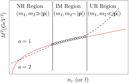
From the previous discussions, it is obvious that the meson Regge trajectories have structure and the expressions of them are complicated. If the Regge trajectories for the mesons in the intermediate region can be approximated by a simple power function, we have from Eqs. (7) and (14)

\displaystyle M^{2}{\sim}l^{\nu},\,n_{r}^{\nu},\quad\left\{\begin{array}[]{cc}\nu=\frac{2a}{a+2},&\text{NR region},\\ \frac{2a}{a+2}<\nu<\frac{2a}{a+1},&\text{IM region},\\ \nu=\frac{2a}{a+1},&\text{UR region}.\end{array}\right.

For the linear confining potential, Eq. (II.2.1) becomes

\displaystyle M^{2}{\sim}l^{\nu},\,n_{r}^{\nu},\quad\left\{\begin{array}[]{cc}\nu=\frac{2}{3},&\text{NR region},\\ \frac{2}{3}<\nu<1,&\text{IM region},\\ \nu=1,&\text{UR region}.\end{array}\right.

In Ref. MartinContreras:2020cyg, the authors associate the index $\nu$ with the average constituent quark mass. From Eq. (II.2.1), we can see that the meson Regge trajectories are concave for the linear confining potential Chen:2018bbr.

As shown in Fig. 1 and in Eq. (II.2.1), in the nonrelativistic (NR) region, the Regge trajectories are significantly nonlinear and can be well approximated by Eq. (10), see more details in Ref. Chen:2018hnx. In the ultrarelativistic (UR) region, it is well-known that the Regge trajectories become approximately linear. In the intermediate (IM) region between the nonrelativistic region and the ultrarelativistic region, the Regge trajectories remain unclear and are expected to be nonlinear. In one word, the approximated Regge trajectories range from the nonlinear form with the exponent $2/3$ to the linear form as the energy region ranges from the nonrelativistic region to the ultrarelativistic region.

The proportion between the nonrelativistic region and the ultrarelativistic region varies with the mesons. For the heavy mesons which are regarded as the nonrelativistic systems, the Regge trajectories take the form in Eq. (10) for small $l$ or $n_{r}$ and they are expected to approximate the linearity for very very large $l$ and $n_{r}$ , see III.2. For the light mesons which are taken as the relativistic systems, the Regge trajectories are linear approximately except for the first few points, see III.4. The heavy-light mesons are special and are usually regarded as the ideal heavy-light systems, see III.3.

II.2.2 Discussions

The mass of a meson can be written as

M=m_{1}+m_{2}+E,

(35)

where $E$ is the interaction energy. In the nonrelativistic limit, the interaction energy $E{\approx}t_{1n}n_{r}^{2/3},\,t_{1l}l^{2/3}$ where $t_{1n}$ and $t_{1l}$ are coefficients, see Eqs. (10) and (51). Using Eq. (35), we have

M^{2}=2t_{1x}(m_{1}+m_{2})x^{2/3}+(m_{1}+m_{2})^{2}+t_{1x}^{2}x^{4/3}\;\;(x=n_{r},l).

(36)

Comparing Eqs. (10) and (36), we have

	$\displaystyle M^{2}-c_{1}=$	$\displaystyle\beta_{x}(x+c_{0})^{2/3}{\ll}2c_{1},$
	$\displaystyle c_{1}=$	$\displaystyle(m_{1}+m_{2})^{2}+t_{1x}^{2}x^{4/3}\geq 0,$		(37)

$c_{1}$ in Eq. (II.2.2) is the modified form in Eq. (12). The formulas in Eq. (II.2.2) are two constraints on the Regge trajectories. In the ultrarelativistic limit, $E{\approx}t_{2n}\sqrt{n_{r}},\,t_{2l}\sqrt{l}$ , see Eq. (17) and Refs. Lucha:1991vn; Brau:2000st. Using Eq. (35), we have

M^{2}=t_{2x}^{2}x+2t_{2x}(m_{1}+m_{2})\sqrt{x}+(m_{1}+m_{2})^{2}\;\;(x=n_{r},l).

(38)

Comparing Eqs. (17) and (38), we have

	$\displaystyle M^{2}-c_{1}=$	$\displaystyle\beta_{x}x{\gg}0.5c_{1},$
	$\displaystyle c_{1}=$	$\displaystyle 2t_{2x}(m_{1}+m_{2})\sqrt{x}+(m_{1}+m_{2})^{2}\geq 0.$		(39)

$c_{1}$ in Eq. (II.2.2) is the modified form in Eq. (12). If the constraints in (II.2.2) are not obeyed, Eq. (17) maybe is not appropriate again.

For the ideal heavy-light systems, $E{\sim}t_{3n}\sqrt{n_{r}},$ $t_{3l}\sqrt{l}$ , see Eqs. (22) and (25). Using Eq. (35), we have

M^{2}=t_{3x}^{2}x+2t_{3x}(m_{1}+m_{2})\sqrt{x}+(m_{1}+m_{2})^{2}\;\;(x=n_{r},l).

(40)

The first term on the right side of Eq. (40) is very small compared with the second term or the third term, then we have the following formulas for the ideal heavy-light systems from Eqs. (23) and (40)

	$\displaystyle M^{2}-c_{1}=$	$\displaystyle\beta_{x}\sqrt{x+c_{0}}{\ll}2c_{1},$
	$\displaystyle c_{1}=$	$\displaystyle(m_{1}+m_{2})^{2}+t_{3x}^{2}x\geq 0.$		(41)

For the common heavy-light systems, the first term in Eq. (40), $t_{3x}^{2}x$ , is comparable with the second term and cannot be neglected, then Eq. (II.2.2) does not hold. For the common heavy-light systems, the Regge-like form (25) Veseli:1996gy; Afonin:2014nya; Afonin:2020bqc; chen2021; Chen:2017fcs; Jia:2019bkr will be better than the simple form (II.2.1).

According to Eqs. (II.2.2), (II.2.2) and (II.2.2), we define one quantity

\xi=\frac{M^{2}-c_{1}}{c_{1}}.

(42)

Then we have

\displaystyle c_{1}{\geq}0,\quad\xi\left\{\begin{array}[]{cc}\ll 2,&\text{NR region or HLS},\\ \gg 0.5,&\text{UR region},\end{array}\right.

where HLS denotes the ideal heavy-light systems. The quantity $\xi$ can be used to show the relation between the masses of the constituents and the interaction energy, similar to Eq. (62).

Physically, the nonlinear formula (10) is obtained in the nonrelativistic limit. Eq. (10) will be inappropriate for the ultrarelativistic region and the parameters $\beta_{x}$ and $c_{1}$ become physically unacceptable, see Tables 5, 6, Eqs. (II.2.1) and (12). In practice, there are limited numbers of points on one Regge trajectory. Mathematically, the parameterized formula $M^{2}=\beta_{x}(x+c_{0})^{2/3}+c_{1}$ where $x=l,\,n_{r}$ can fit one straight line very well like the linear formula $M^{2}={\beta^{\prime}}x+c$ on a finite interval if $c_{0}$ is large. Although $c_{1}$ maybe is negative, the extrapolated data can be good. As $c_{0}$ is large,

M^{2}=\beta(x+c_{0})^{2/3}+c_{1}=\frac{2}{3}\frac{\beta}{c_{0}^{1/3}}x+{\beta}c_{0}^{2/3}+c_{1}+\cdots.

(46)

There is a relation $\beta^{\prime}{\approx}2\beta/(3c_{0}^{1/3})$ . The nonlinear form can be used to fit not only the heavy mesons but also the light mesons, and can give the reasonable predictions, see III.4. The discussions on the nonlinear form in (23) and (25) can be made similarly.

II.3 Consistency of the meson Regge trajectories

II.3.1 Nonrelativistic limit

The nonrelativistic Schrödinger equation with the power law potentials reads

E\psi({\bf r})=\frac{{\bf p}^{2}}{2\mu}\psi({\bf r})+{\sigma}r^{a}\psi({\bf r}),\quad(\sigma,a>0),

(47)

where $\mu=m_{1}m_{2}/(m_{1}+m_{2})$ . The Regge trajectories obtained from Eq. (47) read Brau:2000st; FabreDeLaRipelle:1988zr; Quigg:1979vr; Hall:1984wk

	$\displaystyle E\sim$	$\displaystyle\left[\frac{\sigma^{2}}{(2\mu)^{a}}\right]^{1/(a+2)}\left[\frac{a\pi}{B(1/a,3/2)}\right]^{2a/(a+2)}n_{r}^{2a/(a+2)},$
	$\displaystyle E\sim$	$\displaystyle\frac{2+a}{2}\left[\frac{\sigma^{2}}{(2\mu)^{a}}\right]^{1/(a+2)}\left(\frac{2}{a}\right)^{a/(a+2)}l^{2a/(a+2)}.$		(48)

Although Eq. (II.3.1) is obtained in the limit $l,\,n_{r}\gg 1$ , Eq. (II.3.1) is also appropriate in case of small $l$ or $n_{r}$ FabreDeLaRipelle:1988zr; Quigg:1979vr; Hall:1984wk; Burns:2010qq; Cotugno:2009ys.

As $E/(m_{1}+m_{2})\gg 1$ , the following relations are obtained from Eqs. (35) and (II.3.1),

\displaystyle M^{2}{\sim}E^{2}{\sim}n_{r}^{{4a}/(a+2)},\,l^{{4a}/(a+2)}.

(49)

Eq. (49) is the usually mentioned form as the Regge trajectories from the Schrödinger equation are discussed. According to Eq. (49), the Schrödinger equation with the linear potential produces the Regge trajectories $M^{2}{\sim}$ $l^{4/3}$ , $n_{r}^{4/3}$ which disagree with the experimental data, see Figs. 2, 3 and 4. As $E/(m_{1}+m_{2})\ll 1$ , we obtain from Eqs. (35) and (II.3.1)

\displaystyle M^{2}{\sim}E{\sim}n_{r}^{{2a}/(a+2)},\,l^{{2a}/(a+2)}

(50)

by neglecting term $E^{2}$ . For the linear confining potential $a=1$ , Eq. (50) leads to

\displaystyle M^{2}\sim n_{r}^{{2}/{3}},\,l^{{2}/{3}},

(51)

Eq. (51) takes the same form of the Regge trajectories as Eqs. (II.2.1) and (10). Mathematically, Eq. (49) is applicable in case of $n_{r},\,l\gg 1$ . Physically, the Schrödinger equation is a nonrelativistic equation which is not applicable in the relativistic case, therefore, it is not Eq. (49) but Eq. (50) is appropriate. Eq. (51) is in good agreement with the experimental data, see Fig. 2 and Ref. Chen:2018hnx. The Schrödinger equation can produce the right Regge trajectories for the heavy mesons.

In the nonrelativistic limit, the Regge trajectories [Eqs. (II.2.1) and (10)] obtained from the QSSE are consistent with the Regge trajectories obtained from the Schrödinger equation and from the spinless Salpeter equation. They are also in agreement with the results obtained from the Holography Inspired Stringy Hadron model Sonnenschein:2018fph, the relativistic flux tube model or the loaded flux tube model Burns:2010qq; Cotugno:2009ys, the holographic AdS/QCD context MartinContreras:2020cyg and son on.

II.3.2 Ultrarelativistic limit

In the ultrarelativistic limit, the QSSE will produce the linear Regge trajectories, see Eqs. (16) and (17). It is in agreement with the spinless Salpeter equation Martin:1985hw; Lucha:1991vn; Brau:2000st, the Nambu string model Nambu:1974zg, a first principle Salpeter equation Baldicchi:1998gt, the relativistic Thompson equation Kahana:1993yd, the Holography Inspired Stringy Hadron model Sonnenschein:2018fph, the relativistic flux tube model or the loaded flux tube model Selem:2006nd, the light-front holographic QCD Brodsky:2016yod, the stringlike model Afonin:2014nya, the holographic AdS/QCD context MartinContreras:2020cyg; Karch:2006pv, the holographic model within deformed AdS₅ space metrics FolcoCapossoli:2019imm and so on.

Different dynamic equations or different approximations (appropriate for different energy regions) incorporating with different kinetic terms and different potentials lead to different results. The dynamic equations with p and $r^{a}$ give the $x^{a/(a+1)}$ ( $x=l,\,n_{r}$ ) behavior while those with ${\bf p}^{2}$ and $r^{a}$ give the $x^{2a/(a+2)}$ behavior Chen:2018bbr. Combing the obtained formulas together with masses of constituents leads to different behaviors of the Regge trajectories for different kinds of mesons. We illustrate that the Regge trajectories obtained from the QSSE and that from other approaches are consistent with each other both in the nonrelativistic limit and in the ultrarelativistic limit.

II.4 Virial theorem

In the nonrelativistic limit, by employing the generalized virial theorem chenvp; luo:1991gvt

\left\langle{\bf r}\cdot\frac{\partial{F}}{\partial{\bf r}}\right\rangle=\left\langle{\bf p}\cdot\frac{\partial{F}}{\partial{\bf p}}\right\rangle

(52)

where $F=(m_{1}+m_{2})^{2}+(m_{1}+m_{2})/{\mu}{{\bf p}}^{2}+2(m_{1}+m_{2})V-M^{2}$ to the QSSE (6), we have chenvp

2\left\langle\frac{m_{1}+m_{2}}{\mu}{\bf p}^{2}\right\rangle=a\left\langle 2(m_{1}+m_{2}){\sigma}r^{a}\right\rangle.

(53)

Using Eqs. (6) and (53), we have

M^{2}=(m_{1}+m_{2})^{2}+\frac{a+2}{a}\left\langle\frac{m_{1}+m_{2}}{\mu}{\bf p}^{2}\right\rangle.

(54)

Using Eqs. (6), (7), (35) and (54), we have

E{\sim}\left\langle\frac{{\bf p}^{2}}{\mu}\right\rangle{\sim}\left\langle{\sigma}r^{a}\right\rangle{\sim}n_{r}^{2a/(a+2)},\,l^{2a/(a+2)}.

(55)

In the ultrarelativistic limit, by applying the generalized virial theorem (52) where $F=4{\bf p}^{2}+\lambda{\sigma}^{2}r^{2a}-M^{2}$ to Eq. (13), we have

\left\langle 4{\bf p}^{2}\right\rangle=a\left\langle{\lambda\sigma}^{2}r^{2a}\right\rangle.

(56)

Using Eqs. (13), (14), (35) and (56), we have

M^{2}=4\left\langle{\bf p}^{2}\right\rangle+\left\langle\lambda{\sigma}^{2}r^{2a}\right\rangle=\frac{4a+4}{a}\left\langle{\bf p}^{2}\right\rangle.

(57)

Using Eqs. (14), (35), (56) and (57), we have

E^{2}{\sim}\left\langle{\bf p}^{2}\right\rangle{\sim}\left\langle{\lambda\sigma}^{2}r^{2a}\right\rangle{\sim}n_{r}^{2a/(a+1)},\,l^{2a/(a+1)}.

(58)

Similarly, we have for the ideal heavy-light systems by applying Eq. (52) to Eq. (19)

\left\langle{|{\bf p}|}\right\rangle=a\left\langle{\lambda\sigma}r^{a}\right\rangle.

(59)

Using Eqs. (19), (20), (35) and (59), we have

M^{2}=m_{1}^{2}+2m_{1}\frac{a+1}{a}\left\langle{|{\bf p}|}\right\rangle

(60)

and

E{\sim}\left\langle{|{\bf p}|}\right\rangle{\sim}\left\langle{\sigma}r^{a}\right\rangle{\sim}n_{r}^{a/(a+1)},\,l^{a/(a+1)}.

(61)

The results obtained from the QSSE are in accordance with the results obtained from the Schrödinger equation Quigg:1979vr and from the spinless Salpeter equation Lucha:1989jf. From Eqs. (55), (58) and (61), we can see that the interaction energy, the kinetic energy and the potential are in the same order. Therefore, the $\zeta$ in (62) and $\xi$ in (42) are reasonable and can be used to indicate the energy regions.

III Regge trajectories for mesons

In this section, the energy regions of mesons are discussed and the meson Regge trajectories are fitted individually. Both the nonlinear formula (10) and the linear formula (17) are employed. And only those Regge trajectories with three points or more than three points are presented.

Table 1: The quark masses (in GeV) used in different models. They are used in Tables 2 and 3. The relativistic quark model (RQM) Ebert:2009ub; Ebert:2009ua; Ebert:2011jc, the Godfrey-Isgur model (GIM) Godfrey:1985xj, the second order Bethe-Salpeter formalism (SOBSF) Baldicchi:2003jk and the Holography Inspired Stringy Hadron model (HISHM) Sonnenschein:2018fph are used.

	RQM	GIM	SOBSF	HISHM
$m_{u,d}$	0.33	0.22	0.01	0.060
$m_{s}$	0.5	0.419	0.2	0.400
$m_{c}$	1.55	1.628	1.394	1.490
$m_{b}$	4.88	4.977	4.763	4.700

Some of the fitted resonances could be qualified as a molecular meson-meson state, like most of the axial-vector resonances Roca:2005nm, $f_{2}(1270)$ Molina:2008jw, $f^{\prime}(1525)$ Geng:2008gx, $\rho_{3}(1690)$ , $f_{4}(2050)$ , $\rho_{5}(2350)$ , $f_{6}(2510)$ , $K^{*}_{2}(1430)$ , $K^{*}_{3}(1780)$ , $K^{*}_{4}(2045)$ , $K^{\ast}(52380)$ YamagataSekihara:2010qk; Roca:2010tf. Some of them are accepted as molecules. This possible dominance of the non- $q\bar{q}$ component can change the shape of the Regge trajectory, see for instance Pelaez’s work Pelaez:2017sit and references therein. In this work, we take these resonances as the $q\bar{q}$ states like Refs. Sonnenschein:2018fph; Chen:2018nnr; Chen:2018bbr; Ebert:2009ub; Zyla:2020zbs.

III.1 Energy region

We define a quantity $\zeta$

\zeta=\frac{E}{m_{1}+m_{2}},

(62)

where $E=M-m_{1}-m_{2}$ [Eq. (35)]. $\zeta$ can indicate the energy region of a state. If $\zeta\gg 1$ , the energy region is ultrarelativistic. If $\zeta\ll 1$ , the state is in the nonrelativistic region or is a state of the ideal heavy-light systems. $\zeta{\sim}1$ indicates the intermediate region.

When calculating $\zeta$ , we employ the relativistic quark model (RQM) Ebert:2009ub; Ebert:2009ua; Ebert:2011jc, the Godfrey-Isgur model (GIM) Godfrey:1985xj, the second order Bethe-Salpeter formalism (SOBSF) Baldicchi:2003jk and the Holography Inspired Stringy Hadron model (HISHM) Sonnenschein:2018fph. The quark masses in different models are listed in Table 1. The calculated $\zeta$ for mesons are listed in Tables 2 and 3. For $\zeta$ 1(RQM), $\zeta 2$ (GIM) and $\zeta 3$ (SOBSF), the used meson masses are the theoretical masses in these models, respectively. For $\zeta 4$ (HISHM), the used meson masses are the experimental masses in Ref. Zyla:2020zbs.

Table 2: The orbitally excited meson states used in this work.

aEb

denotes

a\times 10^{b}

. ? denotes the unwell-established states.

{\dagger}

denotes the data calculated by using the spin-averaged centroids.

\ast

means that the experimental masses are used.

Traj.	$n^{2S+1}L_{J}$	$J^{PC}$	Meson	Mass (MeV) Zyla:2020zbs	$\zeta$ 1(RQM)	$\zeta 2$ (GIM)	$\zeta 3$ (SOBSF)	$\zeta 4$ (HISHM)^∗
$\pi/b$	$1^{1}S_{0}$	$0^{-+}$	$\pi^{0}$	$134.9768\pm 0.0005$	$-$ 7.7E $-$ 1	$-$ 6.6E $-$ 1	2.3E+1	1.2E $-$ 1
	$1^{1}P_{1}$	$1^{+-}$	$b_{1}(1235)$	1229.5 ${\pm}$ 3.2	9.1E $-$ 1	1.8E+0	6.6E+1	9.2E+0
	$1^{1}D_{2}$	$2^{-+}$	$\pi_{2}(1670)$	$1670.6^{+2.9}_{-1.2}$	1.5E+0	2.8E+0	8.4E+1	1.3E+1
	$1^{1}F_{3}$	$3^{+-}$	$b_{3}(2030)$ ?	$2032\pm 12$	1.9E+0	3.6E+0	9.9E+1	1.6E+1
	$1^{1}G_{4}$	$4^{-+}$	$\pi_{4}(2250)$ ?	$2250\pm 15$	2.2E+0	4.3E+0	1.1E+2	1.8E+1
$\rho/a$	$1^{3}S_{1}$	$1^{--}$	$\rho(770)$	$775.26\pm 0.25$	1.8E $-$ 1	7.5E $-$ 1	4.1E+1	5.5E+0
	$1^{3}P_{2}$	$2^{++}$	$a_{2}(1320)$	$1316.9\pm 0.9$	1.0E+0	2.0E+0	6.6E+1^†	1.0E+1
	$1^{3}D_{3}$	$3^{--}$	$\rho_{3}(1690)$	$1688.8\pm 2.1$	1.6E+0	2.8E+0	8.4E+1^†	1.3E+1
	$1^{3}F_{4}$	$4^{++}$	$a_{4}(1970)$	$1967\pm 16$	2.1E+0	3.6E+0	9.9E+1^†	1.5E+1
	$1^{3}G_{5}$	$5^{--}$	$\rho_{5}(2350)$ ?	$2330\pm 35$	2.4E+0	4.2E+0	1.1E+2^†	1.8E+1
	$1^{3}H_{6}$	$6^{++}$	$a_{6}(2450)$ ?	$2450\pm 130$	2.8E+0		1.2E+2^†	1.9E+1
$\eta^{\prime}/h$	$1^{1}P_{1}$	$1^{+-}$	$h_{1}(1170)$	$1166\pm 6$	9.1E $-$ 1	1.8E+0		8.7E+0
	$1^{1}D_{2}$	$2^{-+}$	$\eta_{2}(1645)$	$1617\pm 5$	1.5E+0	2.8E+0		1.2E+1
	$1^{1}F_{3}$	$3^{+-}$	$h_{3}(2025)$ ?	$2025\pm 20$	1.9E+0	3.6E+0		1.6E+1
	$1^{1}G_{4}$	$4^{-+}$	$\eta_{4}(2330)$ ?	$2328\pm 38$	2.2E+0	4.3E+0		1.8E+1
$\omega/f$	$1^{3}S_{1}$	$1^{--}$	$\omega(782)$	$782.65\pm 0.12$	1.8E $-$ 1	7.7E $-$ 1		5.5E+0
	$1^{3}P_{2}$	$2^{++}$	$f_{2}(1270)$	$1275.5\pm 0.8$	1.0E+0	1.9E+0		9.6E+0
	$1^{3}D_{3}$	$3^{--}$	$\omega_{3}(1670)$	$1667\pm 4$	1.6E+0	2.8E+0		1.3E+1
	$1^{3}F_{4}$	$4^{++}$	$f_{4}(2050)$	$2018\pm 11$	2.1E+0	3.6E+0		1.6E+1
	$1^{3}G_{5}$	$5^{--}$	$\omega_{5}(2250)$ ?	$2250\pm 70$	2.4E+0	4.2E+0		1.8E+1
	$1^{3}H_{6}$	$6^{++}$	$f_{6}(2510)$ ?	$2465\pm 50$	2.8E+0			2.0E+1
$K$	$1^{1}S_{0}$	$0^{-}$	$K^{0}$	$497.611\pm 0.013$	$-$ 4.2E $-$ 1	$-$ 2.6E $-$ 1	2.1E+0	8.2E $-$ 2
	$1^{1}P_{1}$	$1^{+}$	$K_{1}(1270)$	$1253\pm 7$	5.6E $-$ 1	1.1E+0	5.7E+0	1.7E+0
	$1^{1}D_{2}$	$2^{-}$	$K_{2}(1770)$	$1773\pm 8$	1.1E+0	1.8E+0	7.4E+0	2.9E+0
$K^{*}$	$1^{3}S_{1}$	$1^{-}$	$K^{*}(892)$	$891.66\pm 0.26$	8.1E $-$ 2	4.1E $-$ 1	3.5E+0	9.4E $-$ 1
	$1^{3}P_{2}$	$2^{+}$	$K^{*}_{2}(1430)$	$1427.3\pm 1.5$	7.2E $-$ 1	1.2E+0	5.7E+0^†	2.1E+0
	$1^{3}D_{3}$	$3^{-}$	$K^{*}_{3}(1780)$	$1776\pm 7$	1.2E+0	1.8E+0	7.4E+0^†	2.9E+0
	$1^{3}F_{4}$	$4^{+}$	$K^{*}_{4}(2045)$	$2048^{+8}_{-9}$	1.5E+0	2.3E+0	8.7E+0^†	3.5E+0
	$1^{3}G_{5}$	$5^{-}$	$K^{*}_{5}(2380)$ ?	$2382\pm 24$	1.8E+0	2.7E+0	9.9E+0^†	4.2E+0
$\phi/f^{\prime}$	$1^{3}S_{1}$	$1^{--}$	$\phi(1020)$	$1019.461\pm 0.016$	3.8E $-$ 2	2.2E $-$ 1	1.6E+0	2.7E $-$ 1
	$1^{3}P_{2}$	$2^{++}$	$f_{2}^{\prime}(1525)$	$1517.4\pm 2.5$	5.3E $-$ 1	8.3E $-$ 1	2.7E+0^†	9.0E $-$ 1
	$1^{3}D_{3}$	$3^{--}$	$\phi_{3}(1850)$	$1854\pm 7$	9.5E $-$ 1	1.3E+0	3.6E+0^†	1.3E+0
	$1^{3}F_{4}$	$4^{++}$	$f_{4}(2300)$ ?	$2320\pm 60$	1.3E+0	1.6E+0	4.3E+0^†	1.9E+0
$D$	$1^{1}S_{0}$	$0^{-}$	$D^{0}$	$1864.83\pm 0.05$	$-$ 4.8E $-$ 3	1.7E $-$ 2	3.4E $-$ 1	2.0E $-$ 1
	$1^{1}P_{1}$	$1^{+}$	$D_{1}(2420)^{0}$	$2420.8\pm 0.5$	2.9E $-$ 1	3.2E $-$ 1	7.6E $-$ 1	5.6E $-$ 1
	$1^{1}D_{2}$	$2^{-}$	$D(2740)^{0}$ ?	$2737\pm 12$	4.9E $-$ 1			7.7E $-$ 1
$D^{*}$	$1^{3}S_{1}$	$1^{-}$	$D^{*}(2007)^{0}$	$2006.85\pm 0.05$	6.9E $-$ 2	1.0E $-$ 1	4.4E $-$ 1	2.9E $-$ 1
	$1^{3}P_{2}$	$2^{+}$	$D^{*}_{2}(2460)^{0}$	$2460.7\pm 0.4$	3.1E $-$ 1	3.5E $-$ 1	7.6E $-$ 1^†	5.9E $-$ 1
	$1^{3}D_{3}$	$3^{-}$	$D^{*}_{3}(2750)$ ?	$2763.5\pm 3.4$	5.2E $-$ 1	5.3E $-$ 1		7.8E $-$ 1
$D^{*}_{s}$	$1^{3}S_{1}$	$1^{-}$	$D^{*\pm}_{s}$	$2112.2\pm 0.4$	3.0E $-$ 2	4.1E $-$ 2	3.3E $-$ 1	1.2E $-$ 1
	$1^{3}P_{2}$	$2^{+}$	$D^{*}_{s2}(2573)$	$2569.1\pm 0.8$	2.5E $-$ 1	2.7E $-$ 1	6.0E $-$ 1^†	3.6E $-$ 1
	$1^{3}D_{3}$	$3^{-}$	$D^{*}_{s3}(2860)^{\pm}$ ?	$2860\pm 7$	4.5E $-$ 1	4.3E $-$ 1		5.1E $-$ 1
$\Psi$	$1^{3}S_{1}$	$1^{--}$	$J/\Psi(1S)$	$3096.900\pm 0.006$	$-$ 1.3E $-$ 3	$-$ 4.8E $-$ 2	1.1E $-$ 1	3.9E $-$ 2
	$1^{3}P_{2}$	$2^{++}$	$\chi_{c2}(1P)$	$3556.17\pm 0.07$	1.5E $-$ 1	9.0E $-$ 2	2.7E $-$ 1^†	1.9E $-$ 1
$\eta_{c}$	$1^{1}S_{0}$	$0^{-+}$	$\eta_{c}(1S)$	$2983.9\pm 0.5$	$-$ 3.8E $-$ 2	$-$ 8.8E $-$ 2	7.0E $-$ 2	1.3E $-$ 3
	$1^{1}P_{1}$	$1^{+-}$	$h_{c}(1P)$	$3525.38\pm 0.11$	1.4E $-$ 1	8.1E $-$ 2	2.7E $-$ 1	1.8E $-$ 1
$B$	$1^{1}S_{0}$	$0^{-}$	$B^{\pm}$	$5279.34\pm 0.12$	1.3E $-$ 2	2.2E $-$ 2	1.0E $-$ 1	1.1E $-$ 1
	$1^{1}P_{1}$	$1^{+}$	$B_{1}(5721)^{+}$	$5725.9^{+2.5}_{-2.7}$	9.8E $-$ 2		2.1E $-$ 1	2.0E $-$ 1
$B^{*}$	$1^{3}S_{1}$	$1^{-}$	$B^{*}$	$5324.70\pm 0.21$	2.2E $-$ 2	3.3E $-$ 2	1.2E $-$ 1	1.2E $-$ 1
	$1^{3}P_{2}$	$2^{+}$	$B^{*}_{2}(5747)^{0}$	$5737.2\pm 0.7$	1.0E $-$ 1	1.2E $-$ 1	2.1E $-$ 1^†	2.1E $-$ 1
$B_{s}$	$1^{1}S_{0}$	$0^{-}$	$B_{s}^{0}$	$5366.88\pm 0.14$	$-$ 1.5E $-$ 3	$-$ 1.1E $-$ 3	8.1E $-$ 2	5.2E $-$ 2
	$1^{1}P_{1}$	$1^{+}$	$B_{s1}(5830)^{0}$	$5828.70\pm 0.20$	8.4E $-$ 2		1.8E $-$ 1	1.4E $-$ 1
$B^{*}_{s}$	$1^{3}S_{1}$	$1^{-}$	$B^{*}_{s}$	$5415.4^{+1.8}_{-1.5}$	6.3E $-$ 3	1.0E $-$ 2	9.4E $-$ 2	6.2E $-$ 2
	$1^{3}P_{2}$	$2^{+}$	$B^{*}_{s2}(5840)^{0}$	$5839.86\pm 0.12$	8.6E $-$ 2	9.0E $-$ 2	1.8E $-$ 1^†	1.5E $-$ 1
$\Upsilon$	$1^{3}S_{1}$	$1^{--}$	$\Upsilon(1S)$	$9460.30\pm 0.26$	$-$ 3.1E $-$ 2	$-$ 5.0E $-$ 2	$-$ 6.9E $-$ 3	6.4E $-$ 3
	$1^{3}P_{2}$	$2^{++}$	$\chi_{b2}(1P)$	$9912.21\pm 0.26\pm 0.31$	1.6E $-$ 2	$-$ 5.4E $-$ 3	4.0E $-$ 2^†	5.4E $-$ 2
$\eta_{b}$	$1^{1}S_{0}$	$0^{-+}$	$\eta_{b}(1S)$	$9398.7\pm 2.0$	$-$ 3.7E $-$ 2	$-$ 5.6E $-$ 2	$-$ 1.6E $-$ 2	$-$ 1.4E $-$ 4
	$1^{1}P_{1}$	$1^{+-}$	$h_{b}(1P)$	$9899.3\pm 0.8$	1.4E $-$ 2	$-$ 7.4E $-$ 3	4.0E $-$ 2	5.3E $-$ 2

As shown in Tables 2 and 3, $\zeta>1$ for most of the light mesons. However, $\zeta$ is sometimes small for the first few states on a Regge trajectory for the light mesons. It is suggested that the first few states are neglected as fitting the Regge trajectory to avoid the nonrelativistic effect. For the light mesons, the linear form of a Regge trajectory is a good approximation, see Fig. 4. For the heavy-light mesons, $\zeta{\sim}10^{-1}$ which implies crudely the intermediate region. The fits of the nonlinear Regge trajectories (23) give small or negative $c_{1}$ which are physically meaningless, see III.3 and Fig. 3. For most of the heavy mesons, $\zeta{\sim}10^{-2}$ which indicates the nonrelativistic region. And the nonlinear form of a Regge trajectory (10) will be a good approximation, see Fig. 2.

Table 3: Same as Table 2 except for the radially excited states.

Traj.	$n^{2S+1}L_{J}$	$I(J^{PC})$	Meson	Mass (MeV) Zyla:2020zbs	$\zeta$ 1(RQM)	$\zeta$ 2(GIM)	$\zeta$ 3(SOBSF)	$\zeta$ 4(HISHM)^∗
$\pi$	$1^{1}S_{0}$	$1(0^{-+})$	$\pi^{0}$	$134.9768\pm 0.0005$	$-$ 7.7E $-$ 1	$-$ 6.6E $-$ 1	2.3E+1	1.2E $-$ 1
	$2^{1}S_{0}$		$\pi(1300)$	$1300\pm 100$	9.6E $-$ 1	2.0E+0	6.5E+1	9.8E+0
	$3^{1}S_{0}$		$\pi(1800)$	$1810^{+9}_{-11}$	1.7E+0	3.3E+0	9.0E+1	1.4E+1
	$4^{1}S_{0}$		$\pi(2070)$ ?	$2070\pm 35$	2.1E+0			1.6E+1
	$5^{1}S_{0}$		$\pi(2360)$ ?	$2360\pm 25$	2.6E+0			1.9E+1
$a_{1}$	$1^{3}P_{1}$	$1(1^{++})$	$a_{1}(1260)$	$1230\pm 40$	9.0E $-$ 1	1.8E+0	6.6E+1^†	9.3E+0
	$2^{3}P_{1}$		$a_{1}(1640)$	$1655\pm 16$	1.6E+0	3.1E+0		1.3E+1
	$3^{3}P_{1}$		$a_{1}(2095)$ ?	$2096\pm 17\pm 121$	2.1E+0			1.6E+1
	$4^{3}P_{1}$		$a_{1}(2270)$ ?	$2270^{+55}_{-40}$	2.5E+0			1.8E+1
$\pi_{2}$	$1^{1}D_{2}$	$1(2^{-+})$	$\pi_{2}(1670)$	$1670.6^{+2.9}_{-1.2}$	1.5E+0	2.8E+0	8.4E+1	1.3E+1
	$2^{1}D_{2}$		$\pi_{2}(2005)$ ?	$1963^{+17}_{-27}$	2.0E+0			1.5E+1
	$3^{1}D_{2}$		$\pi_{2}(2285)$ ?	$2285\pm 20\pm 25$	2.4E+0			1.8E+1
$h_{1}$	$1^{1}P_{1}$	$0(1^{+-})$	$h_{1}(1170)$	$1166\pm 6$	9.1E $-$ 1	1.8E+0		8.7E+0
	$2^{1}P_{1}$		$h_{1}(1595)$ ?	$1594^{+18}_{-60}$	1.6E+0	3.0E+0		1.2E+1
	$3^{1}P_{1}$		$h_{1}(1965)$ ?	$1965\pm 45$	2.0E+0			1.5E+1
	$4^{1}P_{1}$		$h_{1}(2215)$ ?	$2215\pm 40$	2.4E+0			1.7E+1
$\omega$	$1^{3}S_{1}$	$0(1^{--})$	$\omega(782)$	$782.65\pm 0.12$	1.8E $-$ 1	7.7E $-$ 1		5.5E+0
	$2^{3}S_{1}$		$\omega(1420)$	$1410\pm 60$	1.3E+0	2.3E+0		1.1E+1
	$3^{3}S_{1}$		$\omega(1650)$	$1670\pm 30$	1.9E+0			1.3E+1
	$4^{3}S_{1}$		$\omega(1960)$ ?	$1960\pm 25$	2.3E+0			1.5E+1
	$5^{3}S_{1}$		$\omega(2290)$ ?	$2290\pm 20$	2.8E+0			1.8E+1
$K$	$1^{1}S_{0}$	$0(0^{-})$	$K^{0}$	$497.611\pm 0.013$	$-$ 4.2E $-$ 1	$-$ 2.6E $-$ 1	2.1E+0	8.2E $-$ 2
	$2^{1}S_{0}$		$K(1460)$	$1482.40\pm 3.58\pm 15.22$	8.5E $-$ 1	1.3E+0	5.7E+0	2.2E+0
	$3^{1}S_{0}$		$K(1830)$ ?	$1874^{+70}_{-120}$	1.5E+0	2.2E+0	8.0E+0	3.1E+0
$\phi$	$1^{3}S_{1}$	$0(1^{--})$	$\phi(1020)$	$1019.461\pm 0.016$	3.8E $-$ 2	2.2E $-$ 1	1.6E+0	2.7E $-$ 1
	$2^{3}S_{1}$		$\phi(1680)$	$1680\pm 20$	7.0E $-$ 1	1.0E+0	3.1E+0	1.1E+0
	$3^{3}S_{1}$		$\phi(2170)$	$2160\pm 80$	1.1E+0		4.2E+0	1.7E+0
$\eta_{c}$	$1^{1}S_{0}$	$0(0^{-+})$	$\eta_{c}(1S)$	$2983.9\pm 0.5$	$-$ 3.8E $-$ 2	$-$ 8.8E $-$ 2	7.0E $-$ 2	1.3E $-$ 3
	$2^{1}S_{0}$		$\eta_{c}(2S)$	$3637.5\pm 1.1$	1.7E $-$ 1	1.1E $-$ 1	2.8E $-$ 1	2.2E $-$ 1
$\Psi$	$1^{3}S_{1}$	$0(1^{--})$	$J/\Psi(1S)$	$3096.900\pm 0.006$	$-$ 1.3E $-$ 3	$-$ 4.8E $-$ 2	1.1E $-$ 1	3.9E $-$ 2
	$2^{3}S_{1}$		$\Psi(2S)$	$3686.10\pm 0.06$	1.9E $-$ 1	1.3E $-$ 1	3.1E $-$ 1	2.4E $-$ 1
	$3^{3}S_{1}$		$\Psi(4040)$	$4039\pm 1$	3.0E $-$ 1	2.6E $-$ 1	4.4E $-$ 1	3.6E $-$ 1
	$4^{3}S_{1}$		$\Psi(4415)$	$4421\pm 4$	4.3E $-$ 1		5.6E $-$ 1	4.8E $-$ 1
$\chi_{c2}$	$1^{3}P_{2}$	$0(2^{++})$	$\chi_{c2}(1P)$	$3556.17\pm 0.07$	1.5E $-$ 1	9.0E $-$ 2	2.7E $-$ 1^†	1.9E $-$ 1
	$2^{3}P_{2}$		$\chi_{c2}(3930)$	$3922.2\pm 1.0$	2.7E $-$ 1	2.2E $-$ 1	4.1E $-$ 1^†	3.2E $-$ 1
$\Upsilon$	$1^{3}S_{1}$	$0(1^{--})$	$\Upsilon(1S)$	$9460.30\pm 0.26$	$-$ 3.1E $-$ 2	$-$ 5.0E $-$ 2	$-$ 6.9E $-$ 3	6.4E $-$ 3
	$2^{3}S_{1}$		$\Upsilon(2S)$	$10023.26\pm 0.31$	2.7E $-$ 2	4.6E $-$ 3	5.1E $-$ 2	6.6E $-$ 2
	$3^{3}S_{1}$		$\Upsilon(3S)$	$10355.2\pm 0.5$	6.1E $-$ 2	4.0E $-$ 2	8.6E $-$ 2	1.0E $-$ 1
	$4^{3}S_{1}$		$\Upsilon(4S)$	$10579.4\pm 1.2$	8.5E $-$ 2	6.8E $-$ 2	1.1E $-$ 1	1.3E $-$ 1
	$5^{3}S_{1}$		$\Upsilon(10860)$	$10885.2^{+2.6}_{-1.6}$	1.1E $-$ 1	9.3E $-$ 2	1.4E $-$ 1	1.6E $-$ 1
	$6^{3}S_{1}$		$\Upsilon(11020)$	$11000\pm 4$	1.4E $-$ 1	1.2E $-$ 1	1.6E $-$ 1	1.7E $-$ 1
$\chi_{b1}$	$1^{3}P_{1}$	$0(1^{++})$	$\chi_{b1}(1P)$	$9892.78\pm 0.26\pm 0.31$	1.4E $-$ 2	$-$ 7.4E $-$ 3	4.0E $-$ 2^†	5.2E $-$ 2
	$2^{3}P_{1}$		$\chi_{b1}(2P)$	$10255.46\pm 0.22\pm 0.50$	5.1E $-$ 2	3.0E $-$ 2	7.7E $-$ 2^†	9.1E $-$ 2
	$3^{3}P_{1}$		$\chi_{b1}(3P)$	$10513.4\pm 0.7$	8.0E $-$ 2			1.2E $-$ 1
$\chi_{b2}$	$1^{3}P_{2}$	$0(2^{++})$	$\chi_{b2}(1P)$	$9912.21\pm 0.26\pm 0.31$	1.6E $-$ 2	$-$ 5.4E $-$ 3	4.0E $-$ 2^†	5.4E $-$ 2
	$2^{3}P_{2}$		$\chi_{b2}(2P)$	$10268.65\pm 0.22\pm 0.50$	5.2E $-$ 2	3.1E $-$ 2	7.7E $-$ 2^†	9.2E $-$ 2
	$3^{3}P_{2}$		$\chi_{b2}(3P)$	$10524.0\pm 0.8$	8.1E $-$ 2			1.2E $-$ 1

III.2 Regge trajectories for the heavy mesons

For the nonlinear fit [Eq. (10)], all states on the Regge trajectories are used. For the linear fit [Eq. (17)], the last four states are used if the data points on the Regge trajectory are equal to or greater than four.

Table 4:

\Upsilon(nS)

states. The experimental masses (in GeV) and the predicted masses fitted by the nonlinear formula

M^{2}=89.55+11.01n_{r}^{2/3}

(Fit1) and by the linear formula

M^{2}=97.90+4.79n_{r}

(Fit2) are listed. When calculating the

\zeta 1

and

\zeta 2

[Eq. (62)],

m_{b}=4.88

Ebert:2009ub; Ebert:2009ua; Ebert:2011jc,

M

are obtained by Fit1 and Fit2, respectively.

	Mass Zyla:2020zbs	Fit1	Fit2	$\zeta$ 1	$\zeta$ 2	$\xi$ 1	$\xi$ 2
$1^{3}S_{1}$	9.46030	9.4631		$-$ 3.0E $-$ 2		0.0	0.0
$2^{3}S_{1}$	10.02326	10.028		2.7E $-$ 2		0.12	0.05
$3^{3}S_{1}$	10.3552	10.345	10.367	6.0E $-$ 2	6.2E $-$ 2	0.20	0.10
$4^{3}S_{1}$	10.5794	10.604	10.596	8.7E $-$ 2	8.6E $-$ 2	0.26	0.15
$5^{3}S_{1}$	10.8852	10.830	10.819	1.1E $-$ 1	1.1E $-$ 1	0.30	0.20
$6^{3}S_{1}$	11.000	11.034	11.039	1.3E $-$ 1	1.3E $-$ 1	0.36	0.24
$7^{3}S_{1}$		11.221	11.253	1.5E $-$ 1	1.5E $-$ 1	0.41	0.29
$8^{3}S_{1}$		11.395	11.464	1.7E $-$ 1	1.7E $-$ 1	0.45	0.34
$9^{3}S_{1}$		11.558	11.671	1.8E $-$ 1	2.0E $-$ 1	0.49	0.39
$10^{3}S_{1}$		11.713	11.875	2.0E $-$ 1	2.2E $-$ 1	0.53	0.44
$11^{3}S_{1}$		11.860	12.075	2.2E $-$ 1	2.4E $-$ 1	0.57	0.49
$12^{3}S_{1}$		12.000	12.272	2.3E $-$ 1	2.6E $-$ 1	0.61	0.54
$13^{3}S_{1}$		12.135	12.465	2.4E $-$ 1	2.8E $-$ 1	0.64	0.59
$14^{3}S_{1}$		12.265	12.656	2.6E $-$ 1	3.0E $-$ 1	0.68	0.64
$15^{3}S_{1}$		12.390	12.844	2.7E $-$ 1	3.2E $-$ 1	0.71	0.68

As shown in Fig. 2 and Tables 2 and 3, $\zeta$ [Eq. (62)] are small for the heavy mesons especially for the bottomonia which indicates the nonrelativistic region. The fitted nonlinear Regge trajectories agree very well with the experimental data. As the linear formula is used to fit the Regge trajectories for the heavy mesons, $c_{1}$ which should be small becomes very large. It suggests that the linear formula is not a good match for the nonrelativistic energy region.

For the heavy mesons especially for the bottomonia, $\xi 1$ [Eq. (42)] calculated by the nonlinear formula and $\xi 2$ by the linear formula are consistent with each other and obey the constraints in (II.2.2), see Tables 4, 5 and 6. As shown in Table 4, $\zeta\ll 1$ and $\xi\ll 2$ are in agreement. It is expected that all bottomonia including the observed states and the states observed in the future will be in the nonrelativistic region. The predicted masses of the highly excited states of the bottomonia are also listed in Table 4.

III.3 Regge trajectories for the heavy-light mesons

For both the nonlinear fits [Eqs. (10) and (23)] and the linear fits [Eq. (17)], all states on the Regge trajectories are used. Only the Regge trajectories with three or more points are presented.

The quantity $\zeta{\sim}10^{-1}$ for the heavy-light mesons, see Table 2 and III.1. The Regge trajectories for the heavy-light mesons are nonlinear. As the nonlinear formula (23), which is derived in case of the ideal heavy-light systems, is employed to fit the Regge trajectories for the heavy-light mesons, the fitted parameter $c_{1}$ is small or negative, see Fig. 3. It disagrees with the constraints in Eq. (II.2.2). As the nonlinear formula (10) is applied, $\xi 1$ is greater than one which does not obey the constraints in (II.2.2). $\xi 2$ calculated by the fitted linear formula in (17) neither obeys the constraints. Moreover, $\xi 1$ calculated by the nonlinear form and $\xi 2$ by the linear form contradict, see Tables 5 and 6. All these clues indicate that the heavy-light mesons are not the ideal heavy-light systems, not in the nonrelativistic region nor in the ultrarelativistic region. However, they can be regarded brute-forcely as the ideal heavy-light systems or as being in the intermediate energy region,

III.4 Regge trajectories for the light mesons

For the nonlinear fit, all states on the Regge trajectories are used. For the linear fit, the last four states on a Regge trajectory are used if the data points on the Regge trajectory are equal to or greater than four.

As shown in Tables 5 and 6, $\xi$ calculated by the linear formula is much greater than $0.5$ while $\xi$ calculated by the nonlinear formula is negative. These results are consistent and show that the light mesons are in the relativistic region. ( $c^{\prime}$ and $\xi 2$ for the linear $\eta/h$ Regge trajectory are negative, which can be adjusted if the first data point is included.)

The light mesons are the relativistic systems, see Tables 2 and 3. The Regge trajectories for the light mesons can be well described by the linear formula, see Fig. 4. As applying the nonlinear formula appropriate for the nonrelativistic region to fit the Regge trajectories for the light mesons, $c_{1}$ , which should be positive according to Eq. (II.2.2), becomes negative, see Tables 5 and 6. $c_{0}$ becomes very large and $c_{0}=100$ in this work. $\beta_{x}$ which should be small becomes large, see Tables 5, 6, Eqs. (II.2.1) and (12). These imply that the nonlinear formula (10) does not match the ultrarelativistic energy region. However, as shown in Fig. 4, the nonlinear formula (10) can give good extrapolated predictions because (10) is appropriate mathematically, see II.2.2.

According to Tables 2, 3, 5 and 6, $\pi$ mesons are in the relativistic region. However, the Regge trajectories for $\pi$ are nonlinear, see Figs. 4 and 4. The cause of the nonlinearity remains unclear. It maybe is a coincidence that the Regge trajectories for $\pi$ can be well described by the nonlinear formula (10).

III.5 Discussions on $\xi$

Both $\zeta$ [Eq. (62)] and $\xi$ [Eq. (42)] can measure the relation between the interaction energy and the masses of constituents. $\zeta$ can give a clear classification of the energy regions while there exist ambiguity sometimes for $\xi$ , see II.2.2 and III.1. Calculating the quantity $\zeta$ needs the masses of the constituents which vary with models while calculating $\xi$ does not need the masses.

For an unknown Regge trajectory, it is better to employ the linear formula and the nonlinear formula to calculate the quantity $\xi$ to check the energy region. As $\xi\ll 2$ , the mesons will be nonrelativistic and the nonlinear formula (10) is appropriate. As $\xi\gg 0.5$ or $\xi<0$ , the mesons will be relativistic and the linear formula is good. If $\xi$ calculated by two different formulas are in contradiction, the mesons will be regarded rudely as being in the intermediate region, see III.3, Tables 5 and 6.

IV Dependence of $\beta$ on mass and the string tension $\sigma$

The slope $\beta$ in the Regge trajectories is an important quantity Basdevant:1984rk. In the ultrarelativistic limit, masses of the constituents are supposed to approach zero. It agrees with the well-known knowledge that the Regge trajectories for the light mesons is approximately linear and the slope depends only on the string tension $\sigma$ , see Eqs. (17) and (18). In the nonrelativistic limit, the Regge trajectories is significantly nonlinear and $\beta$ depends not only on the string tension but also on the masses of the constituents, see Eqs. (10) and (II.2.1). In the intermediate region, it is expected that $\beta$ depends likewise both on the masses of constituents and on the string tension, but the dependence on the masses are expected to weaken as the masses decrease.

Use a linear formula

M^{2}=\beta^{\prime}x+c^{\prime}_{1}\;(x=n_{r},\,l)

(63)

to fit a nonlinear Regge trajectory which can be described by

M^{2}=\beta_{1}(x+c_{0})^{\nu}+c_{1}\;\text{or}\;M^{2}=\beta_{2a}x+\beta_{2b}x^{\nu}+c_{2},

(64)

where $\beta^{\prime}$ and $\beta_{2a}$ are independent of the masses of the constituents while $\beta_{1}$ and $\beta_{2b}$ depend on the masses. By differentiating Eqs. (63) and (64), we have

\beta^{\prime}=\nu{\beta_{1}}(x_{0}+c_{0})^{\nu-1}\;\text{or}\;\beta^{\prime}=\beta_{2a}+\nu\beta_{2b}x^{\nu-1},

(65)

where $x_{0}$ is a point on the Regge trajectory.

In case of the linear fit, Eq. (63) is employed. The fitted slopes are almost a constant for the light mesons. They increase for the heavy-light mesons and become very large for the heavy mesons. It is in agreement with Refs. Nielsen:2018ytt; Ebert:2009ub; Ebert:2009ua; Ebert:2011jc; Sonnenschein:2014jwa; Abreu:2020ttf; Abreu:2020wio; Kher:2017mky. The fitted slopes of the radial trajectories $\beta^{\prime}_{n_{r}}$ are about 1.2 for the light unflavored mesons, become 1.63 for the $K$ trajectory, 3.26 for the $\psi$ trajectory and 4.79 for the $\Upsilon$ trajectory. $\beta^{\prime}_{l}$ are about 1.1 for the light unflavored mesons, $1.45$ for the $K$ trajectory, $1.80$ for the $D^{\ast}$ trajectory, 3.06 for the $\psi$ trajectory and 8.76 for the $\Upsilon$ trajectory, see Tables 5 and 6. Eq. (65) explains why the $\beta^{\prime}$ of (63) increases with the masses of the constituents. For example, for the $\psi/\chi_{c}$ trajectory $\beta_{l}=3.53$ , $c_{0}=0.08$ and $x_{0}=0.375$ give $\beta^{\prime}_{l}=3.06$ according to Eq. (65), which is in agreement with the fitted value.

In case of the nonlinear fit, the first formula in (64) with $\nu=2/3$ is applied, which is appropriate for the heavy mesons, see Fig. 2. The fitted slopes $\beta_{l}$ and $\beta_{n_{r}}$ are in accordance with the theoretical predictions, see Ref. Chen:2018hnx. As discussed in the subsection II.2.2, the first formula in (64) can also be applied to fit the Regge trajectories for the heavy-light mesons and for the light mesons, see Figs. 3 and 4. According to Eq. (46), there is a relation between the slopes of a nonlinear fit and the slopes of a linear fit. For example, for the $\rho/a$ trajectory $\beta^{\prime}_{l}=1.15$ calculated by using Eq. (46) is in agreement with the fitted value $\beta^{\prime}_{l}=1.10$ .

V Conclusions

In this work, we investigate the structure of the meson Regge trajectories based on the quadratic form of the spinless Salpeter-type equation. The form of the meson Regge trajectories is complicated and depends on the energy region. In the nonrelativistic limit, the approximated form of the Regge trajectories is $M^{2}=\beta_{x}(x+c_{0})^{2/3}+c_{1}$ [Eq. (10)]. In the ultrarelativistic limit, it is well known that the Regge trajectories can be well described by the linear formula $M^{2}=\beta_{x}x+c_{1}$ [Eq. (17)]. In the intermediate energy region, the simple form of the Regge trajectories remains unclear and is expected to be nonlinear. We show that the Regge trajectories obtained from different approaches are consistent with each other in the nonrelativistic limit and in the ultrarelativistic limit.

By employing the nonlinear formulas and the linear formula, the Regge trajectories for different mesons are given. As a Regge trajectory formula is unsuitable for the energy region, the fitted parameters neither have explicit physical meanings nor obey the constraints [Eq. (II.2.2)], however, the fitted Regge trajectory can give the satisfactory extrapolated predictions if the employed formula is appropriate mathematically. Using a linear formula to fit the Regge trajectories for the heavy mesons, $\beta_{x}$ and $c_{1}$ become very large. Conversely, using a nonlinear formula to fit the light mesons, $c_{1}$ becomes negative.

Moreover, the slopes of the fitted linear formula will increase for the heavy-light mesons and become very large for the heavy mesons. We show that the masses of the constituents will come into the slope and explain why the slopes of the fitted linear Regge trajectories vary with the masses of the constituents as the linear formula is used to fit the Regge trajectories for the heavy-light mesons and for the heavy mesons, see Eq. (65).

Acknowledgements We are very grateful to the anonymous referees for the valuable comments and suggestions. This work is supported by the Natural Science Foundation of Shanxi Province of China under Grant no. 201901D111289.

Data Avilability Statement This manuscript has no associated data or the data will not be deposited. [Authors’ comment: All data are included in the paper.]

Table 5: The radial Regge trajectories fitted by the nonlinear formula

M^{2}=\beta_{n_{r}}(n_{r}+c_{0})^{2/3}+c_{1}

(Fit1) and by the linear formula

M^{2}=\beta^{\prime}_{n_{r}}n_{r}+c^{\prime}

c^{\prime}=\beta^{\prime}_{l}l+c^{\prime}_{1}

(Fit2).

\beta^{\prime}_{l}{\approx}1.1

for

a_{1}

\pi_{2}

and

h_{1}

\beta^{\prime}_{l}\approx 5.1

for

\chi_{b1}

and

\chi_{b2}

by fitting the data in Ref. Ebert:2011jc. For the nonlinear fit, all points are used. For the linear fit, only the last four points are used if the points on the Regge trajectory are more than four. For the nonlinear fit, the effect of

l

is absorbed into

c_{0}

, see Eq. (II.2.2). For the linear fit, the terms containing

n_{r}

and

l

should be written explicitly, see Eq. (II.2.2).

{\dagger}

denotes that

\xi 1

reads

0.48

by using the global fit Chen:2018hnx.

Traj.	Fit1	Fit2	$\xi 1$	$\xi 2$
	$(\beta_{n_{r}},c_{0},c_{1})$	$(\beta^{\prime}_{n_{r}},c^{\prime})$	$n_{r}=1$	$n_{r}=1$
$\pi$	$(2.78,\;0.80,\;-2.38)$	$(1.26,\;0.54)$	$-$ 1.73	2.33
$a_{1}$	$(3.23,\;3.59,\;-6.05)$	$(1.26,\;1.56)$	$-$ 1.47	5.13
$\pi_{2}$	$(8.49,\;100,\;-180.)$	$(1.22,\;2.74)$	$-$ 1.02	6.33
$h_{1}$	$(4.42,\;13.5,\;-23.7)$	$(1.20,\;1.37)$	$-$ 1.11	8.52
$\omega$	$(3.06,\;4.33,\;-7.52)$	$(1.08,\;0.76)$	$-$ 1.24	1.42
$K$	$(2.29,\;0.10,\;-0.25)$	$(1.63,\;0.35)$	$-$ 9.76	4.66
$\phi$	$(12.7,\;100,\;-272.)$	$(1.81,\;1.03)$	$-$ 1.01	1.76
$D$ Chen:2018nnr	$(4.05,\;0.25,\;1.85)$	$(2.68,\;3.62)$	2.54	0.74
$\psi$	$(6.19,\;0.77,\;4.39)$	$(3.26,\;9.87)$	$2.06^{{\dagger}}$	0.33
$\Upsilon$	$(11.0,\;0.0,\;89.5)$	$(4.79,\;97.9)$	0.12	0.05
$\chi_{b1}$	$(9.67,\;0.27,\;93.8)$	$(6.33,\;98.2)$	0.12	0.12
$\chi_{b2}$	$(9.59,\;0.28,\;94.1)$	$(6.25,\;98.6)$	0.12	0.12

Table 6: The orbital Regge trajectories fitted by the nonlinear formula

M^{2}=\beta_{l}(l+c_{0})^{2/3}+c_{1}

(Fit1) and by the linear formula

M^{2}=\beta^{\prime}_{l}l+c^{\prime}

(Fit2), where

c^{\prime}=\beta^{\prime}_{n_{r}}n_{r}+c^{\prime}_{1}

n_{r}=0

. For the nonlinear fit, all points are used. For the linear fit, only the last four points are used if the points on the Regge trajectory are more than four. For the nonlinear fit, the effect of

n_{r}

is absorbed into

c_{0}

, see Eq. (II.2.2). For the linear fit, the terms containing

n_{r}

and

l

should be written explicitly, see Eq. (II.2.2).

Traj.	Fit1	Fit2	$\xi 1$	$\xi 2$
	$(\beta_{l},c_{0},c_{1})$	$(\beta^{\prime}_{l},c^{\prime})$	$l=1$	$l=1$
$\pi/b$	$(2.83,\;1.52,\;-3.73)$	$(1.20,\;0.38)$	$-$ 1.41	3.16
$\rho/a$	$(5.36,\;30.3,\;-51.5)$	$(1.10,\;0.68)$	$-$ 1.03	1.62
$\eta/h$	$(9.59,\;100,\;-207)$	$(1.37,\;-0.04)$	$-$ 1.00	$-$ 34.3
$\omega/f$	$(7.81,\;100,\;-168)$	$(1.09,\;0.69)$	$-$ 1.01	1.58
$K$	$(10.1,\;100,\;-218)$	$(1.45,\;0.21)$	$-$ 1.00	6.90
$K^{\ast}$	$(8.35,\;100,\;-179)$	$(1.20,\;0.78)$	$-$ 1.01	1.54
$\phi/f^{\prime}$	$(9.91,\;100,\;-213)$	$(1.42,\;0.92)$	$-$ 1.01	1.54
$D$	$(2.85,\;0.12,\;2.78)$	$(2.01,\;3.60)$	1.11	0.56
$D^{\ast}$	$(2.97,\;0.49,\;2.18)$	$(1.80,\;4.10)$	1.78	0.44
$D^{\ast}_{s}$	$(2.86,\;0.29,\;3.21)$	$(1.86,\;4.55)$	1.06	0.41
$\psi/\chi_{c}$ Chen:2018hnx	$(3.53,\;0.08,\;8.92)$	$(3.06,\;9.59)$	0.42	0.32
$\Upsilon/\chi_{b}$ Chen:2018hnx	$(9.27,\;0.02,\;88.9)$	$(8.76,\;88.5)$	0.11	0.10

References

(1) G. F. Chew and S. C. Frautschi, Phys. Rev. Lett. 7, 394-397 (1961) doi:10.1103/PhysRevLett.7.394
(2) G. F. Chew and S. C. Frautschi, Phys. Rev. Lett. 8, 41-44 (1962) doi:10.1103/PhysRevLett.8.41
(3) P. D. B. Collins, An Introduction to Regge Theory and High-Energy Physics (Cambrige University Press, London, 1977). doi:10.1017/CBO9780511897603
(4) Y. Nambu, Phys. Rev. D 10, 4262 (1974) doi:10.1103/PhysRevD.10.4262
(5) J. Polchinski and M. J. Strassler, Phys. Rev. Lett. 88, 031601 (2002) doi:10.1103/PhysRevLett.88.031601 [arXiv:hep-th/0109174 [hep-th]].
(6) M. Nielsen, S. J. Brodsky, G. F. de Téramond, H. G. Dosch, F. S. Navarra and L. Zou, Phys. Rev. D 98, no.3, 034002 (2018) doi:10.1103/PhysRevD.98.034002 [arXiv:1805.11567 [hep-ph]].
(7) M. G. Olsson, S. Veseli and K. Williams, Phys. Rev. D 51, 5079-5089 (1995) doi:10.1103/PhysRevD.51.5079 [arXiv:hep-ph/9410405 [hep-ph]].
(8) D. E. Kahana, K. M. Maung and J. W. Norbury, Phys. Rev. D 48, 3408-3409 (1993) doi:10.1103/PhysRevD.48.3408
(9) W. Lucha, F. F. Schoberl and D. Gromes, Phys. Rept. 200, 127-240 (1991) doi:10.1016/0370-1573(91)90001-3
(10) M. Baldicchi and G. M. Prosperi, Phys. Lett. B 436, 145-152 (1998) doi:10.1016/S0370-2693(98)00830-2 [arXiv:hep-ph/9803390 [hep-ph]].
(11) A. Martin, Z. Phys. C 32 359, 315-322 (1986) doi:10.1007/BF01551832
(12) J. Sonnenschein and D. Weissman, Eur. Phys. J. C 79, no.4, 326 (2019) doi:10.1140/epjc/s10052-019-6828-y [arXiv:1812.01619 [hep-ph]].
(13) A. Inopin and G. S. Sharov, Phys. Rev. D 63, 054023 (2001) doi:10.1103/PhysRevD.63.054023 [arXiv:hep-ph/9905499 [hep-ph]].
(14) A. M. Badalian and B. L. G. Bakker, Phys. Rev. D 100, no.3, 034010 (2019) doi:10.1103/PhysRevD.100.034010 [arXiv:1901.10280 [hep-ph]].
(15) S. J. Brodsky, G. F. de Téramond, H. G. Dosch and C. Lorcé, Phys. Lett. B 759 (2016), 171-177 doi:10.1016/j.physletb.2016.05.068 [arXiv:1604.06746 [hep-ph]].
(16) A. Selem and F. Wilczek, doi:10.1142/9789812773524_0030 [arXiv:hep-ph/0602128 [hep-ph]].
(17) J. T. Londergan, J. Nebreda, J. R. Pelaez and A. Szczepaniak, Phys. Lett. B 729, 9-14 (2014) doi:10.1016/j.physletb.2013.12.061 [arXiv:1311.7552 [hep-ph]].
(18) M. M. Brisudova, L. Burakovsky and J. T. Goldman, Phys. Rev. D 61, 054013 (2000) doi:10.1103/PhysRevD.61.054013 [arXiv:hep-ph/9906293 [hep-ph]].
(19) M. N. Sergeenko, Z. Phys. C 64, 315-322 (1994) doi:10.1007/BF01557404
(20) M. N. Sergeenko, Phys. Atom. Nucl. 56, 365-371 (1993)
(21) S. Veseli and M. G. Olsson, Phys. Lett. B 383, 109-115 (1996) doi:10.1016/0370-2693(96)00721-6 [arXiv:hep-ph/9606257 [hep-ph]].
(22) S. S. Afonin and I. V. Pusenkov, Phys. Rev. D 90, no.9, 094020 (2014) doi:10.1103/PhysRevD.90.094020 [arXiv:1411.2390 [hep-ph]].
(23) S. S. Afonin, doi:10.1142/9789811219313_0018 [arXiv:2009.05378 [hep-ph]].
(24) G. Cotugno, R. Faccini, A. D. Polosa and C. Sabelli, Phys. Rev. Lett. 104, 132005 (2010) doi:10.1103/PhysRevLett.104.132005 [arXiv:0911.2178 [hep-ph]].
(25) T. J. Burns, F. Piccinini, A. D. Polosa and C. Sabelli, Phys. Rev. D 82, 074003 (2010) doi:10.1103/PhysRevD.82.074003 [arXiv:1008.0018 [hep-ph]].
(26) M. A. Martin Contreras and A. Vega, Phys. Rev. D 102 (2020) no.4, 046007 doi:10.1103/PhysRevD.102.046007 [arXiv:2004.10286 [hep-ph]].
(27) J. K. Chen (2021), in preparation.
(28) A. E. Inopin, [arXiv:hep-ph/0110160 [hep-ph]], and references therein.
(29) J. K. Chen, Eur. Phys. J. C 78, no.3, 235 (2018) doi:10.1140/epjc/s10052-018-5718-z
(30) J. K. Chen, Eur. Phys. J. C 78, no.8, 648 (2018) doi:10.1140/epjc/s10052-018-6134-0
(31) J. K. Chen, Phys. Lett. B 786, 477-484 (2018) doi:10.1016/j.physletb.2018.10.022 [arXiv:1807.11003 [hep-ph]].
(32) M. Baldicchi, A. V. Nesterenko, G. M. Prosperi, D. V. Shirkov and C. Simolo, Phys. Rev. Lett. 99 (2007), 242001 doi:10.1103/PhysRevLett.99.242001 [arXiv:0705.0329 [hep-ph]].
(33) M. Baldicchi, A. V. Nesterenko, G. M. Prosperi and C. Simolo, Phys. Rev. D 77 (2008), 034013 doi:10.1103/PhysRevD.77.034013 [arXiv:0705.1695 [hep-ph]].
(34) N. Brambilla, E. Montaldi and G. M. Prosperi, Phys. Rev. D 54 (1996), 3506-3525 doi:10.1103/PhysRevD.54.3506 [arXiv:hep-ph/9504229 [hep-ph]].
(35) J. K. Chen, Acta Phys. Pol. B 47, 1155 (2016)
(36) J. K. Chen, Rom. J. Phys. 62, 119 (2017)
(37) S. Tomonaga, Quantum Mechanics, Volume I: Old Quantum Theory (North-Holland Publishing Company, Amsterdam, 1962)
(38) F. Brau, Phys. Rev. D 62, 014005 (2000) doi:10.1103/PhysRevD.62.014005 [arXiv:hep-ph/0412170 [hep-ph]].
(39) I.S. Gradshteyn, I.M. Ryzhik, Table of Integrals, Series, and Products, corrected and, enlarged edition (Academic Press, New York, 1980)
(40) K. Chen, Y. Dong, X. Liu, Q. F. Lü and T. Matsuki, Eur. Phys. J. C 78, no.1, 20 (2018) doi:10.1140/epjc/s10052-017-5512-3 [arXiv:1709.07196 [hep-ph]].
(41) D. Jia, W. N. Liu and A. Hosaka, Phys. Rev. D 101, no.3, 034016 (2020) [arXiv:1907.04958 [hep-ph]].
(42) M. Fabre De La Ripelle, Phys. Lett. B 205 (1988), 97-102 doi:10.1016/0370-2693(88)90406-6
(43) C. Quigg and J. L. Rosner, Phys. Rept. 56 (1979), 167-235 doi:10.1016/0370-1573(79)90095-4
(44) R. L. Hall, Phys. Rev. D 30 (1984), 433-436 doi:10.1103/PhysRevD.30.433
(45) A. Karch, E. Katz, D. T. Son and M. A. Stephanov, Phys. Rev. D 74 (2006), 015005 doi:10.1103/PhysRevD.74.015005 [arXiv:hep-ph/0602229 [hep-ph]].
(46) E. Folco Capossoli, M. A. Martín Contreras, D. Li, A. Vega and H. Boschi-Filho, Chin. Phys. C 44, no.6, 064104 (2020) doi:10.1088/1674-1137/44/6/064104 [arXiv:1903.06269 [hep-ph]].
(47) Z. F. Luo and X. J. Qiu, J. Phys. G: Nucl. Part. Phys. 18, 221-224 (1992)
(48) W. Lucha and F. F. Schoberl, Phys. Rev. Lett. 64 (1990), 2733 doi:10.1103/PhysRevLett.64.2733
(49) D. Ebert, R. N. Faustov and V. O. Galkin, Phys. Rev. D 79 (2009), 114029 doi:10.1103/PhysRevD.79.114029 [arXiv:0903.5183 [hep-ph]].
(50) D. Ebert, R. N. Faustov and V. O. Galkin, Eur. Phys. J. C 66 (2010), 197-206 doi:10.1140/epjc/s10052-010-1233-6 [arXiv:0910.5612 [hep-ph]].
(51) D. Ebert, R. N. Faustov and V. O. Galkin, Eur. Phys. J. C 71 (2011), 1825 doi:10.1140/epjc/s10052-011-1825-9 [arXiv:1111.0454 [hep-ph]].
(52) S. Godfrey and N. Isgur, Phys. Rev. D 32 (1985), 189-231 doi:10.1103/PhysRevD.32.189
(53) M. Baldicchi and G. M. Prosperi, doi:10.1142/9789812702845_0014 [arXiv:hep-ph/0310213 [hep-ph]].
(54) L. Roca, E. Oset and J. Singh, Phys. Rev. D 72, 014002 (2005) doi:10.1103/PhysRevD.72.014002 [arXiv:hep-ph/0503273 [hep-ph]].
(55) R. Molina, D. Nicmorus and E. Oset, Phys. Rev. D 78, 114018 (2008) doi:10.1103/PhysRevD.78.114018 [arXiv:0809.2233 [hep-ph]].
(56) L. S. Geng and E. Oset, Phys. Rev. D 79, 074009 (2009) doi:10.1103/PhysRevD.79.074009 [arXiv:0812.1199 [hep-ph]].
(57) J. Yamagata-Sekihara, L. Roca and E. Oset, Phys. Rev. D 82, 094017 (2010) [erratum: Phys. Rev. D 85, 119905 (2012)] doi:10.1103/PhysRevD.82.094017 [arXiv:1010.0525 [hep-ph]].
(58) L. Roca and E. Oset, Phys. Rev. D 82, 054013 (2010) doi:10.1103/PhysRevD.82.054013 [arXiv:1005.0283 [hep-ph]].
(59) J. R. Pelaez and A. Rodas, Eur. Phys. J. C 77, no.6, 431 (2017) doi:10.1140/epjc/s10052-017-4994-3 [arXiv:1703.07661 [hep-ph]].
(60) P. A. Zyla et al. [Particle Data Group], PTEP 2020 (2020) no.8, 083C01 doi:10.1093/ptep/ptaa104
(61) J. L. Basdevant and S. Boukraa, Z. Phys. C 28, 413 (1985) doi:10.1007/BF01413604
(62) J. Sonnenschein and D. Weissman, JHEP 08, 013 (2014) doi:10.1007/JHEP08(2014)013 [arXiv:1402.5603 [hep-ph]].
(63) L. M. Abreu, F. M. d. Júnior and A. G. Favero, Phys. Rev. D 102, no.3, 034002 (2020) doi:10.1103/PhysRevD.102.034002 [arXiv:2007.07849 [hep-ph]].
(64) L. M. Abreu, F. M. da Costa Júnior and A. G. Favero, Phys. Rev. D 101, no.11, 116016 (2020) doi:10.1103/PhysRevD.101.116016 [arXiv:2004.10736 [hep-ph]].
(65) V. Kher, N. Devlani and A. K. Rai, Chin. Phys. C 41, no.9, 093101 (2017) doi:10.1088/1674-1137/41/9/093101 [arXiv:1705.08248 [hep-ph]].

Structure of the meson Regge trajectories

Abstract

I Introduction

II Structure of the meson Regge trajectories

II.1 QSSE

II.2 Regge trajectories obtained from the QSSE

II.2.1 Regge trajectories

II.2.2 Discussions

II.3 Consistency of the meson Regge trajectories

II.3.1 Nonrelativistic limit

II.3.2 Ultrarelativistic limit

II.4 Virial theorem

III Regge trajectories for mesons

III.1 Energy region

III.2 Regge trajectories for the heavy mesons

III.3 Regge trajectories for the heavy-light mesons

III.4 Regge trajectories for the light mesons

III.5 Discussions on ξ\xi

IV Dependence of β\beta on mass and the string tension σ\sigma

V Conclusions

References

III.5 Discussions on $\xi$

IV Dependence of $\beta$ on mass and the string tension $\sigma$