Phase-dependent fluctuations of resonance fluorescence near the coherent population trapping condition

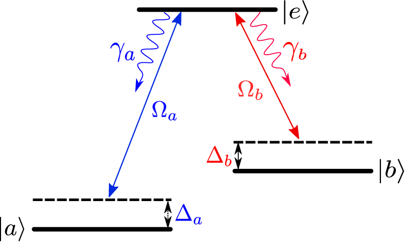
Our system, pictorially represented in Fig. 1, consists of a $\Lambda$-type three-level atom ($\Lambda$-3LA) with a single excited state $|e\rangle$ coupled by a monochromatic laser with Rabi frequency $\Omega_{a}$ to the ground state $|a\rangle$ and decay rate $\gamma_{a}$, and to a long-lived state $|b\rangle$ by a monochromatic laser with Rabi frequency $\Omega_{b}$ and decay rate $\gamma_{b}$. Decay from $|b\rangle$ to $|a\rangle$ is dipole-forbidden. Henceforth, the fields driving the $|a\rangle\to|e\rangle$ and $|b\rangle\to|e\rangle$ transitions will be referred to as the probe and control fields. We define the atomic operators as $\hat{\sigma}_{jk}=|j\rangle\langle k|$.

Under the above considerations, the system’s evolution, in free space, and in the frame rotating at the laser frequencies, $\nu_{a}$ and $\nu_{b}$, is governed by the master equation $\dot{\tilde{\rho}}(t)=-i[\hat{H},\tilde{\rho}]+\sum_{j}\frac{\gamma_{j}}{2}\mathcal{L}_{\hat{\sigma}_{je}}[\tilde{\rho}]$, in which

is the atom-laser Hamiltonian, and $\Delta_{j}=\omega_{ej}-\nu_{j}$ labels the individual atom-laser detunings. Dissipation is accounted for by the action of the Lindblad generator $\mathcal{L}_{\hat{O}}[\tilde{\rho}]=2\hat{O}\tilde{\rho}\hat{O}^{\dagger}-\hat{O}^{\dagger}\hat{O}\tilde{\rho}-\tilde{\rho}\hat{O}^{\dagger}\hat{O}$, with $\hat{O}=\hat{\sigma}_{je}$. With the help of the relationship $\hat{\sigma}_{jk}\hat{\sigma}_{lm}=\hat{\sigma}_{jm}\delta_{kl}$, the master equation can be explicitly recast as

With the relation $\langle\hat{\sigma}_{jk}\rangle=\tilde{\rho}_{kj}$, Eq. (2) allows us to arrive at the following set of linear equations for populations:

with $\gamma=\gamma_{a}+\gamma_{b}$, and coherences:

The solution to these equations (a set of nine Bloch equations) is to be obtained numerically and their structure will facilitate the assessment of the sought correlation functions via the quantum regression formula, combined with the employment of matrix methods. For later use, we define the values of the atomic operators in the steady state as

Besides, in order for our findings to be possibly put to the test in a given realization, we shall consider the decays $\gamma_{a}=14.7$ MHz and $\gamma_{b}=5.4$ MHz, observed in ${}^{138}\mathrm{Ba}^{+}$ ions GRS+09; SHG+10; DNG+15. Although a more accurate description of Barium resonance fluorescence would entail considering its multilevel structure, being composed of eight energy levels, it suffices for our purposes to deal with the simplified three-level system as a proxy for specifying the relevant allowed dipole transitions that take part in the dynamics. Parenthetically, the isolation of a single three-level configuration can be implemented through a proper optical pumping arrangement.

The $\Lambda$-type three-level atom is an archetypal system that readily fulfills the necessary conditions for coherent population trapping (CPT) to take place Arimondo; FlIM05. In such a scenario, the system is known to evolve towards the trapping state $|u\rangle=(\Omega_{b}|a\rangle-\Omega_{a}|b\rangle)/\sqrt{\Omega_{a}^{2}+\Omega_{b}^{2}}$ that turns out to be decoupled from the lasers, thereby dropping the long-term excited-state population $\alpha_{ee}$ to nearly zero. The manifestation of this effect is exemplified in the upper panel of Fig. 2, where the steady state population of the excited state is shown as a function of both the detuning and Rabi frequency of the probe laser ($e\to a$ transition); the values of the parameters associated with the control field are, henceforth, taken to be fixed and the same as those reported in SHG+10, namely, $\Omega_{b}/\gamma_{a}\approx 2.15$ and $\Delta_{b}/\gamma_{a}\approx 2.38$. In accord with the well-established prescription to determine the frequency region around which the atom is essentially transparent to the incoming probe field, the so-called Raman resonance condition, the probe detuning must be such that $\Delta_{a}\approx\Delta_{b}$ is satisfied; the role of the probe intensity $\Omega_{a}$ is that of slightly modifying the width of such a transparent frequency window. Its location is also depicted in the lower panel of Fig. 2 showing the cross sectional profile of the upper figure (black line) at $\Omega_{a}/\gamma_{a}\approx 1.12$ where, in turn, we can observe the complete depopulation of the excited state at $\Delta_{a}/\gamma_{a}\approx 2.38$ (dashed vertical line); the populations of the $|a\rangle$ and $|b\rangle$ states are also added as a supplementary view of their behavior as functions of the probe detuning.

The foregoing was not the actual condition under which the experiments SHG+10 were performed, but instead the detuning was chosen so as to fit the value of the corresponding saturation parameter, $\Omega_{j}^{2}/(\gamma_{j}^{2}+\Delta_{j}^{2})$, and taken to be $\sim 0.1$ for the $a\to e$ transition. This choice gives rise to a detuning of about $\Delta_{a}/\gamma_{a}\approx 3.4$, the location of which being also indicated in the figure (dotted-dashed vertical line); the saturation parameter associated with the control field was set to $0.8$. So, for this particular choice of probe and control detunings that drive the $a\to e$ transition out of the Raman resonance condition, the complete depopulation of the $|e\rangle$ state can be avoided or delayed, a working situation that will permit us to study the non-classical properties of the scattered light we seek to assess. It is worth commenting that if, instead, the $a\to e$ transition were driven more strongly than the $b\to e$ one, such that $\Omega_{a}>\Omega_{b}$, for general detunings, the population would end up in the $|b\rangle$ state, with $\Omega_{b}\ll\gamma_{a}$. So then, the strong transition would be turned off due to lack of recycling population to $|e\rangle$.

So, having established the present configuration of laser intensities and frequencies, we find it pertinent, at this stage, to depict the stationary power spectrum of the re-emitted light obtained by use of the Wiener-Khintchine formula

i.e., the Fourier transform of the autocorrelation function of the dipole field, $\langle\hat{\sigma}_{ea}(0)\hat{\sigma}_{ae}(\tau)\rangle_{ss}$, where $ss$ indicates that the process is stationary; the prefactor $(\pi\alpha_{ee})^{-1}$ normalizes the integral over all frequencies. For convenience, the spectrum is separated into its coherent and incoherent parts, namely, $S(\omega)=S_{coh}(\omega)+S_{inc}(\omega)$, as a result of considering the dynamics of the atomic variables to be split into their mean and fluctuations, viz. $\hat{\sigma}_{jk}(t)=\alpha_{jk}+\Delta\hat{\sigma}_{jk}(t)$, with $\langle\Delta\hat{\sigma}_{jk}(t)\rangle=0$. In doing so, we get

where $\alpha_{ea}=\langle\hat{\sigma}_{ea}\rangle_{ss}$, and

the former being the coherent constituent of the spectrum owing to elastic scattering, and the latter the incoherent part of the spectrum that is brought about by atomic fluctuations. The main features of the $\Lambda$-type three-level atom spectrum have already been studied from the weak to the strong field limit, both theoretically and experimentally SSA+96. Figure 3 shows a three dimensional view of the incoherent part of the spectrum associated with the $e\to a$ transition, the one of interest to us, as a function of the probe intensity (upper panel) and the detuning (lower panel); details of the steps involved in the calculations herein via the matrix analysis are included in Appendix A. The general spectral profile can be understood in terms of dressed-state configuration that follows from properly diagonalizing the atom-field Hamiltonian Cohen92, emphasizing the fact that, above saturation, the spectrum displays the appearance of Rabi sidebands as the intensity field increases, as one can see in the upper panel of the figure. By setting the Rabi frequency at, say, $\Omega_{a}/\gamma_{a}=1.12$, such sidebands become sufficiently conspicuous and the dependency of their profile upon the detuning is shown in the lower panel.

Resonance fluorescence is a highly non-linear process, preventing its description in terms of quasi-probability distributions, i.e., it does not admit a Fokker-Planck type of equation. The non-linearity leads to non-Gaussian fluctuations, thus giving rise to non-vanishing odd-order moments. Autocorrelation functions such as that for the spectrum, $\langle\sigma_{ea}(0)\sigma_{ae}(\tau)\rangle$; squeezing, $\langle\Delta\sigma_{\phi}(0)\Delta\sigma_{\phi}(\tau)\rangle$; and photon-photon correlation, $\langle\sigma_{ea}(0)\sigma_{ea}(\tau)\sigma_{ae}(\tau)\sigma_{ae}(0)\rangle$, are of even-order and, as such, time-symmetric DeCC02. These functions do not address the non-Gaussianity of the field’s fluctuations.

In amplitude-intensity correlations, Eq.(14), on the other hand, such a symmetry is not guaranteed: being different observables, the outcome will be dependent on the time order of measurements. For instance, the quadrature is measured (preselected) for $\tau\geq 0$ and the intensity for $\tau\leq 0$ (quadrature is post-selected), a process in which time-asymmetry is expected to be revealed. Moreover, this correlation would allow us to explore non-classical features of light beyond squeezing and antibunching.

Applying the time and normal operator orderings in Eq.(14) we arrive at the following expressions for positive and negative time intervals,

The asymmetry in time revealed by CHD, as shown in Fig. 5, is an indicative of non-Gaussian noise. The correlation (14) contains a product of three dipole operators or, more generally, three field amplitude operators. This means that $h_{\phi}(\tau)$ provides access up to third order fluctuations; since these are non-Gaussian, this third-order correlation does not vanish. To better distinguish the asymmetry and the size of these fluctuations, we proceed, as we did with the spectrum, to split the dipole dynamics into its mean plus fluctuations, $\hat{\sigma}_{jk}=\alpha_{\phi}+\Delta\hat{\sigma}_{jk}$ hmcb10,

where

and

are the components of, respectively, second- and third-order in the dipole fluctuations of $h_{\phi}(\tau)$, where $\Delta\hat{\sigma}_{\phi}=(\Delta\hat{\sigma}_{ea}e^{-i\phi}+\Delta\hat{\sigma}_{ae}e^{i\phi})/2$ is the quadrature fluctuation operator. Fluctuations are said to be Gaussian if $h_{\phi}^{(3)}(\tau)\to 0$, which can occur when the transition is weakly driven.

For positive time intervals between photon and quadrature detections, we get

We show in Fig. 6 the foregoing second- and third-order correlations. For both quadratures, the third-order constituent (blue lines) represents the main contribution, almost that of the total $h_{\phi}(\tau)$ (black lines). This is understandable from the fact that we are above the saturation threshold GCRH17, a regime where non-Gaussian fluctuations become significant. In this regime the dipole $\alpha_{ea}$, indicative of the coherence induced by the laser, is small; most of the total emission is incoherent. This observation can be quantitatively revealed from the fact that $h_{\phi}(0)=0$ (just as it occurs for photon correlations in resonance fluorescence), which leads to the relation GCRH17

For strong fields, $|\alpha_{ea}|\ll\alpha_{ee}$, $h_{\phi}^{(3)}(0)$ reaches its extremal value -2, thereby making the dipole factor in Eq.(20) small compared to the third-order term.

Even though the splitting itself cannot be directly realizable from the experimental viewpoint via the measurement scheme, it provides us with valuable theoretical information to be able to discern the actual contribution to the system’s fluctuations.

For $\tau<0$, we want to stress the fact that the outcome of CHD correlation should be taken with special care: it is to be interpreted as the measurement of the intensity after the detection of the amplitude. Thus, as previously underlined, the asymmetry results from the different fluctuations of the light’s amplitude and intensity. Time and normal operator ordering leads to

i. e., the correlation is only of second order in the dipole fluctuations, albeit with $\Delta\hat{\sigma}_{ee}$ instead of the quadrature amplitude $\Delta\hat{\sigma}_{\phi}$ fluctuation operator.

The initial motivation for CHD was to detect squeezing from weak sources, such as cavity QED CCFO00; FOCC00. Resonance fluorescence is also a producer of weakly squeezed light WaZo81; CoWZ84. In order to produce light in a squeezed state, a non-classical property of light, these sources must be weakly driven, so that the third-order fluctuations discussed above are small. As we will see later, the remaining second-order signal is related to the spectrum of squeezing. CHD, hence, gives non-classical criteria in the time domain as resulting of violation of the classical inequalities CCFO00; FOCC00

where the second relation is derived for Gaussian fluctuations. More recently, it was found that light in a coherent state obeys GCRH17

light outside these bounds violates Poissonian statistics. According to these criteria, we see in Figs. 5 and 6 that both the in-phase ($\phi=0$, continuous line) and out-of-phase ($\phi=\pi/2$, dashed line) quadratures of the field display a non-classical character, violating one or more inequalities. The fact that $h_{\phi}(0)=0$ already shows a non-classical feature, akin to antibunching in the intensity fluctuations. Also, moderately strong fields easily drive $h_{\phi}(\tau)$ out of the classical bounds.

We see, then, that CHD clearly reveals non-classicality of quadratures in the time domain. Let us now proceed to scrutinize the spectral profile of amplitude-intensity correlations in the frequency domain.

References

- (1) E. Arimondo, Progress in Optics, 35, 257 (1996).
- (2) M. Fleischhauer, A. Imamoglu and J. P. Marangos, Rev. Mod. Phys. 77 633 (2005).
- (3) L. Slodička, G. Hétet, S. Gerber, M. Hennrich, and R. Blatt, Phys. Rev. A 105 153604 (2010).
- (4) J. Hwang, M. Pototschig, R. Lettow, G. Zumofen, A. Renn, S. Götzinger, and V. Sandoghdar, Nature (London) 460, 76 (2009).
- (5) D. F. Walls and P. Zoller, Phys. Rev. Lett. 47 709 (1981).
- (6) M. J. Collett, D. F. Walls, P. Zoller, Optics Commun. 52, 145-149 (1984).
- (7) C. H. H. Schulte, J. Hansom, A. E. Jones, C. Matthiesen, C. Le Gall, and M. Atatüre, Nature 525, 222 (2015).
- (8) W. Vogel, Phys. Rev. Lett. 67, 2450-2452 (1991).
- (9) W. Vogel, Phys. Rev. A 51, 4160 (1995).
- (10) B. Kühn, W. Vogel, M. Mraz, S. Köhnke, and B. Hage, Phys. Rev. Lett. 118, 153601 (2017).
- (11) S. Gerber, D. Rotter, L. Slodička, J. Eschner, H. J. Carmichael, and R. Blatt, Phys. Rev. Lett. 102, 183601 (2009).
- (12) E. V. Shchukin and W. Vogel, Phys. Rev. A 72, 043808 (2005).
- (13) E. V. Shchukin and W. Vogel, Phys. Rev. Lett. 96, 200403 (2006).
- (14) H. J. Carmichael, H. M. Castro-Beltran, G. T. Foster, and L. A. Orozco, Phys. Rev. Lett. 85, 1855 (2000).
- (15) G. T. Foster, L. A. Orozco, H. M. Castro-Beltran, and H. J. Carmichael, Phys. Rev. Lett. 85, 3149 (2000).
- (16) For a review on CHD see H. J. Carmichael, G. T. Foster, L. A. Orozco, J. E. Reiner, and P. R. Rice, in Progress in Optics 46, E. Wolf, ed. (Elsevier, 2004).
- (17) H. M. Castro-Beltran, Opt. Commun. 283, 4680 (2010).
- (18) H. M. Castro-Beltran, L. Gutierrez, and L. Horvath, Appl. Math. Inf. Sci. 9, 2849 (2015).
- (19) A. Denisov, H. M. Castro-Beltran, and H. J. Carmichael, Phys. Rev. Lett. 88, 243601 (2002).
- (20) H. M. Castro-Beltran, R. Roman-Ancheyta, and L. Gutierrez, Phys. Rev. A, 93, 033801 (2016).
- (21) E. R. Marquina-Cruz and H. M. Castro-Beltran, Laser Phys. 18, 157 (2008).
- (22) L. Gutierrez, H. M. Castro-Beltran, R. Roman-Ancheyta, and L. Horvath, J. Opt. Soc. Am. B 34, 2301 (2017).
- (23) Q. Xu, E. Greplova, B. Julsgaard, and K. Mølmer, Phys. Scripta 90, 128004 (2015).
- (24) Q. Xu and K. Mølmer, Phys. Rev. A 92, 033830 (2015).
- (25) S. Gammelmark, B. Julsgaard, and K. Mølmer, Phys. Rev. Lett. 111, 160401 (2013).
- (26) F. Wang, X. Feng, and C. H. Oh, Laser Phys. Lett. 13, 105201 (2016).
- (27) O. de los Santos-Sánchez. Front. Phys. 14, 61601 (2019).
- (28) T. Zhao, Z.-A. Peng, G.-Q. Yang, G.-M. Huang, and G.-X. Li, Optics Express 28, 379 (2020).
- (29) E. A. M. Nuñez-Portela, A. T. Grier, K. Jungmann, A. Mohanty, N. Valappol, and L. Willmann, Phys. Rev. A, 91, 060501(R) (2015).
- (30) Y. Stalgies, I. Siemers, B. Appasamy, T. Altevogt, and P. E. Toscheck, Europhys. Lett. 35, 259 (1996).
- (31) C. Cohen-Tannoudji, J. Dupont-Roc, and G. Grynberg, Atom-Photon Interactions: Basic Processes and Applications (Wiley, New York, 1992).
- (32) H. J. Carmichael, Statistical Methods in Quantum Optics 1: Master Equations and Fokker-Planck Equations (Springer-Verlag, Berlin, 2002).
- (33) H. J. Carmichael, J. Opt. Soc. Am. B 4, 1588 (1987).