Dynamics and Control of a Flapping Wing UAV with Abdomen Undulation Inspired by Monarch Butterfly

Consider a flapping wing UAV that is composed of a body, an abdomen, and two wings attached to the body. Here, we assume that the head and thorax are combined into a single rigid body referred to as the body.

Define an inertial frame $\mathcal{F}_{I}=\{\mathbf{i}_{x},\mathbf{i}_{y},\mathbf{i}_{z}\}$, which is compatible to the NED (north-east-down) frame. The various components of this model are described below.

• •

  Body: The origin of the body-fixed frame $\mathcal{F}_{B}=\{\mathbf{b}_{x},\mathbf{b}_{y},\mathbf{b}_{z}\}$is defined at the mass center of the body. Its attitude is given by $R\in\mathsf{SO(3)}$ and the position of mass center is given by $x\in\mathbb{R}^{3}$ in $\mathcal{F}_{I}$. The kinematics of the attitude is

  $\displaystyle\dot{R}=R\hat{\Omega},$

  (1)

  where $\Omega\in\mathbb{R}^{3}$ is the angular velocity of the body resolved in $\mathcal{F}_{B}$.

• •

  Right wing: Let $\mathcal{F}_{R}=\{\mathbf{r}_{x},\mathbf{r}_{y},\mathbf{r}_{z}\}$ be the frame fixed to the right wing at its root. And let $\mathcal{F}_{S}=\{\mathbf{s}_{x},\mathbf{s}_{y},\mathbf{s}_{z}\}$ be the stroke frame obtained by translating the origin of $\mathcal{F}_{B}$ to the center of the left and the right wing roots, and rotating it about $\mathbf{b}_{y}$ by a fixed angle $\beta\in[-\pi,\pi)$. Let $\mu_{R}\in\mathbb{R}^{3}$ be the fixed vector from the origin of $\mathcal{F}_{B}$ to that of $\mathcal{F}_{R}$.

  The attitude of the right wing relative to $\mathcal{F}_{S}$, namely $Q_{R}\in\mathsf{SO(3)}$ is described by 1–3–2 Euler angles $(\phi_{R}(t),\psi_{R}(t),\theta_{R}(t))$ (Figure 1) as

  $\displaystyle Q_{R}=\exp(\beta\hat{e}_{2})\exp(\phi_{R}\hat{e}_{1})\exp(-\psi_{R}\hat{e}_{3})\exp(\theta_{R}\hat{e}_{2}),$

  and its time-derivative is $\dot{Q}_{R}=Q_{R}\hat{\Omega}_{R}$ for $\Omega_{R}\in\mathbb{R}^{3}$.

• •

  Left Wing: Similarly, for the left wing,

  $$Q_{L}=\exp(\beta\hat{e}_{2})\exp(-\phi_{L}\hat{e}_{1})\exp(\psi_{L}\hat{e}_{3})\exp(\theta_{L}\hat{e}_{2}),$$

  with the set of Euler-angles $(\phi_{L}(t),\psi_{L}(t),\theta_{L}(t))$, and $\dot{Q}_{L}=Q_{L}\hat{\Omega}_{L}$ for $\Omega_{L}\in\mathbb{R}^{3}$.

• •

  Abdomen: The abdomen is considered as a rigid body attached to the body via a spherical joint. The frame fixed to the abdomen is $\mathcal{F}_{A}=\{\mathbf{a}_{x},\mathbf{a}_{y},\mathbf{a}_{z}\}$, and its attitude relative to the body is denoted by $Q_{A}\in\mathsf{SO(3)}$ with $\dot{Q}_{A}=Q_{A}\hat{\Omega}_{A}$ for $\Omega_{A}\in\mathbb{R}^{3}$. When there is no rotation relative to the body, its orientation is identical to $\mathcal{F}_{B}$.

The motion of the wing relative to the body is referred to as wing kinematics. As described above and depicted in Figure 1, it is defined by three angles, referred to as the flapping angle, the pitch angle, and the deviation angle. Here we adopt the particular wing kinematics model presented in [12].

Let $f\in\mathbb{R}$ be the frequency of flapping in $\mathrm{Hz}$ and $T=\frac{1}{f}$ be the period in seconds. The flapping angle is given by a smoothed triangular waveform,

where $\phi_{m}\in\mathbb{R}$ is the amplitude, $\phi_{0}\in\mathbb{R}$ is the offset, and $0<\phi_{K}\leq 1$ determines waveform shape (sinusoidal when $\phi_{K}\rightarrow 0$; triangular when $\phi_{K}\rightarrow 1$). The initial pitch angle is $\phi(0)=\phi_{m}+\phi_{0}$. During $0\leq t\leq\frac{T}{2}$, it decreases to $\phi(\frac{T}{2})=-\phi_{m}+\phi_{0}$. According to the sign convention illustrated at Figure 1, it represents an upstroke when $0\leq t\leq\frac{T}{2}$, and a downstroke when $\frac{T}{2}\leq t\leq T$.

The pitch angle is given by a hyperbolic function,

where $\theta_{m}\in\mathbb{R}$ is the amplitude of pitching, $\theta_{0}\in\mathbb{R}$ is the offset, $\theta_{C}\in(0,\infty)$ determines the waveform (sinusoidal when $\theta_{C}\rightarrow 0$; step function when $\theta_{C}\rightarrow\infty$), and $\theta_{a}\in(-\pi,\pi)$ describes phase offset (advance rotation for $\theta_{a}>0$; symmetric rotation for $\theta_{a}=0$; delayed rotation for $\theta_{a}<0$). The value of $\theta_{C}$ is related to the duration of wing pitch reversal.

Finally, the deviation angle is given by

where $\psi_{m}\in\mathbb{R}$ is the amplitude, $\psi_{0}\in\mathbb{R}$ is the offset, and the parameter $\psi_{a}\in(-\pi,\pi)$ is the phase offset. The parameter $\psi_{N}$ is either 1 or 2: $\psi_{N}=1$ corresponds to one oscillation per a flapping period, and $\psi_{N}=2$ is for a figure-eight motion.

Next, we present the expressions for the aerodynamic forces and moments generated by the wings. Here, the blade-element theory [13] is utilized along with a quasi-steady aerodynamics assumption. More explicitly, it implies that the aerodynamic force generated by an infinitesimal chord is independent of the span-wise velocity component, and that the force and moment generated are equivalent to those for steady motion at the same instantaneous velocity and angle of attack.

Since the expression for the left wing can be similarly obtained, only the right wing is discussed below. Consider an infinitesimal segment on the right wing at a distance $r$ from the wing root. In $\mathcal{F}_{R}$, the relative velocity of the aerodynamic center of this chord element ($c(r)$), projected to avoid span-wise components is

where $v_{\mathrm{wind}}\in\mathbb{R}^{3}$ is the uniform wind velocity in $\mathcal{F}_{I}$. From this, the angle of attack $\alpha_{R}(r)\in[0,\frac{\pi}{2}]$ is

Let $\rho\in\mathbb{R}$ be the atmospheric density, and let $C_{L},C_{D}\in\mathbb{R}$ as the lift and drag coefficients, respectively. The corresponding aerodynamic forces and moment generated by the infinitesimal wing segment are

The total lift, drag, and moment of the right wing are obtained by integrating above span-wise for $r\in[0,l]$, for the right wing span $l\in\mathbb{R}^{3}$. Compared with the other models considering the uniform force over the wing, the above expression captures the span-wide variations of the angle of attack and the aerodynamic forces, which are critical for FWUAVs with relative large wings flapping at a low frequency.

The configuration of the above flapping wing UAV model is described by $g=(x,R,Q_{R},Q_{L},Q_{A})$, and as such, it is a mechanical system evolving on the Lie group $\mathsf{G}=\mathbb{R}^{3}\times\mathsf{SO(3)}^{4}$, whose Lie algebra is simply $\mathfrak{g}=\mathbb{R}^{3}\times\mathfrak{so}(3)^{4}\simeq\mathbb{R}^{3}\times(\mathbb{R}^{3})^{4}$. Therefore, its equation of motion can be formulated by Lagrangian mechanics on a manifold [14].

The kinematics equation on $\mathsf{G}$ is given by

for $\xi=(\dot{x},\Omega,\Omega_{R},\Omega_{L},\Omega_{A})\in\mathfrak{g}$. Let $\mathbf{J}:\mathsf{G}\times\mathfrak{g}\rightarrow\mathfrak{g}^{*}$ be a symmetric, positive-definite inertia tensor. And define $(\mathbf{K}_{g}(\xi))(\cdot):\mathsf{G}\times\mathfrak{g}\rightarrow\mathfrak{g}^{*}$ such that $\mathsf{T}_{e}^{*}\mathsf{L}_{g}\cdot\mathbf{D}_{g}\mathbf{J}_{g}(\xi)\cdot\chi=(\mathbf{K}_{g}(\xi))(\chi)=\mathbf{K}_{g}(\xi)\chi$. Consider a Lagrangian $L:\mathsf{G}\times\mathfrak{g}\rightarrow\mathbb{R}$ given by $L(g,\xi)=\frac{1}{2}\langle\mathbf{J}_{g}(\xi),\xi\rangle-U(g)$ for a potential $U:\mathsf{SO(3)}\rightarrow\mathbb{R}$. The corresponding Euler–Lagrange equations [14] are written as

where $\mathbf{f}\in\mathbb{R}^{15}$ represents the effects of the aerodynamic forces and the internal torques at the joint. The explicit expressions for each term of the above equation are available in [11].

The above equation is driven by the control torque acting on each joint. Instead, it is assumed that the motion of the wings, abdomen, and body are prescribed, i.e., $(R(t),Q_{R}(t),Q_{L}(t),Q_{A}(t))$ are given as functions of time. This is common in the literature, as the inertia of the wings are relatively small. Substituting these, the reduced equation of motion for the position is

where $F_{i}=L_{i}+D_{i}\in\mathbb{R}^{3}$ denotes the resultant aerodynamic force at each component, $m\in\mathbb{R}$ is the total mass, and $g\in\mathbb{R}$ is the gravitational acceleration.

In short, (12) describes how the position of FWUAV evolves over time for a given wing kinematics and abdomen undulation, while capturing the dynamic coupling between components, and the aerodynamic forces and moments.

For numerical analyses presented in the remainder of this paper, the wing morphological parameters and the mass properties are chosen to be similar with those of Monarch, and the specific values are summarized in [11]. For the aerodynamic coefficients, we adopt the experimental results presented in [15, 16] as summarized below.

where $\alpha^{\circ}=\alpha\frac{180}{\pi}$. Next, the aerodynamic force generated by the body and the abdomen is ignored, i.e., $F_{A}=0$. This is reasonable as the projected surface area of the body and the abdomen is negligible compared with the wings.

When generating a periodic motion, the body and the abdomen are assumed to undulate. This is motivated by the flight characteristics of live Monarch butterfly exhibiting a nontrivial pitching motion of the body and the abdomen [11]. Specifically, the attitude of the body is defined as $R(t)=\exp(\theta_{B}(t)\hat{e}_{2})$, where the body pitch angle is

for fixed parameters $\theta_{B_{m}}$, $\theta_{B_{a}}$, and $\theta_{B_{0}}\in\mathbb{R}$.

Similarly, the attitude of the abdomen relative to the body is $Q_{A}(t)=\exp(\theta_{A}(t)\hat{e}_{2})$, where

for $\theta_{A_{m}},\theta_{A_{a}},\theta_{A_{0}}\in\mathbb{R}$.

An optimization problem to generate this motion is formulated as follows,

• •

  The objective function is the absolute amount of energy input into the system and corresponding power required:

  $$J=w_{1}\int_{0}^{T}|E(t)|dt+w_{2}\int_{0}^{T}|\dot{E}(t)|dt,$$

  (15)

  where $w_{1},w_{2}\in\mathbb{R}$ are positive weighting factors, and $E(t)\in\mathbb{R}$ is composed of the kinetic energy and the gravitational potential energy:

  $$E(t)=\frac{1}{2}m\left\|\dot{x}(t)\right\|^{2}-mge_{3}^{T}x(t).$$

  (16)

• •

  The optimization parameters are

  • –

    flapping frequency: $f$

  • –

    stroke plane angle: $\beta$

  • –

    wing kinematics: $(\phi_{m},\phi_{K},\phi_{0})$, $(\theta_{m},\theta_{C},\theta_{0},\theta_{a})$, $(\psi_{m},\psi_{0},\psi_{a})$

  • –

    body undulation: $(\theta_{B_{m}},\theta_{B_{0}},\theta_{B_{a}})$

  • –

    abdomen undulation $(\theta_{A_{m}},\theta_{A_{0}},\theta_{A_{a}})$

  • –

    initial velocity: $\dot{x}(0)$

• •

  There are equality constraints to ensure periodicity:

  $$x(0)=x(T),\quad\dot{x}(0)=\dot{x}(T).$$

  (17)

  There is an inequality constraint for feasibly flapping:

  $$|\phi_{m}|+|\phi_{0}|<\pi/2.$$

  (18)

  All of the optimization parameters are bounded by prescribed limits.

It is considered that the motion of the left wing is always symmetric to the right wing. The above parameter optimization problem is solved via MATLAB global optimization tools, such as multistart or particleswarm. The optimized parameters are summarized at Table I, and the corresponding periodic maneuver is illustrated at Figure 2.

To further study the effects of abdomen, another optimization is carried out while assuming that the abdomen does not undulate relative to the body, i.e., $\theta_{A}(t)=\theta_{A_{0}}$ for a fixed parameter $\theta_{A_{0}}$. The resulting optimized parameters are summarized at the second column of Table I, where the optimal value of the objective function is increased by $23\%$ when the abdomen is fixed. The corresponding variation of $E$ and $\dot{E}$ are presented at Figure 3.(a). It is shown that the abdomen undulation reduces the variation of the total energy and its time-derivatives.

Next, the torque required at the joint of the wing $(\tau_{R},\tau_{L})$ and the torque at the joint connecting the body and the abdomen $\tau_{A}$ are reconstructed from (11). The corresponding power at the joints are computed as $P_{R}=\tau_{R}^{T}(Q_{R}\Omega_{R})$, $P_{A}=\tau_{A}^{T}(Q_{A}\Omega_{A})$. The change of power over a flapping period is illustrated at Figure 3.(b), which shows $1.8\%$ reduction of the power with abdomen undulation.

The torque at abdomen for the case with relative abdomen undulation can be modeled by a torsional spring/ damper at the joint. Considering $\tau_{A}(t)=-k\theta_{A}(t)-c\dot{\theta}_{A}(t)+\tau_{0}$ and using a least squares fit for the data, we obtain $k=$9.4262\text{\times}{10}^{-05}$,\ c=$7.6634\text{\times}{10}^{-07}$,\ \tau_{0}=$4.1641\text{\times}{10}^{-05}$$ (see the subfigure (d)). These show that the abdomen undulation may reduce the total energy and the power consumption required for hovering. Interestingly, such beneficial effects may be achieved by allowing the abdomen to passively undulate after the muscle connecting the body and the abdomen is modeled as a torsional spring/damper.

Let $\mathbf{x}\in\mathbb{R}^{6}$ be the congregated state of the position and the velocity, i.e., $\mathbf{x}=(x,\dot{x})\in\mathbb{R}^{6}$. Also, let $\mathbf{x}_{d}=(x_{d},\dot{x}_{d})\in\mathbb{R}^{6}$ be the periodic orbit for hovering constructed in the preceding subsection, satisfying $\mathbf{x}_{d}(t+T)=\mathbf{x}_{d}(t)$ for any $t>0$.

The perturbation of the state $\mathbf{x}$ from the periodic orbit $\mathbf{x}_{d}$ is denoted by $\delta\mathbf{x}=\mathbf{x}-\mathbf{x}_{d}=(\delta x,\delta\dot{x})\in\mathbb{R}^{6}$. Ignoring the higher-order terms, the evolution of the perturbation is described by the equation of motion, namely (12) linearized about $\mathbf{x}_{d}$ as

where $R(t),Q_{R}(t),Q_{L}(t)$ corresponds to the body undulation and the wing kinematics for the periodic orbit, and $\delta F_{R},\delta F_{L}$ represent the variation of the aerodynamic force due to the perturbation of the velocity. For example,

where $\delta L_{R},\delta D_{R}$ can be computed from (7), (8) and

Utilizing these, the linearized equations of motion, (19), (20) can be rearranged into the following matrix form:

where the matrix $\mathbf{A}(t)\in\mathbb{R}^{6\times 6}$ is periodic with the period $T$. While the solution of (22), namely $\delta\mathbf{x}(t)$ is not periodic in general, it can be written as a linear combination of a set of periodic solutions multiplied by so-called characteristic multiplier [17].

More specifically, let $\Psi(t)\in\mathbb{R}^{6\times 6}$ be the solution of the matrix differential equation $\dot{\Psi}=\mathbf{A}\Psi$, starting from a nonsigular $\Psi(0)\in\mathbb{R}^{6\times 6}$. The matrix $\Psi(t)$ is referred to as the fundamental matrix of (22). Using the fact that $\mathbf{A}(t)$ is periodic, one can show that $\Psi(t+T)$ is also a fundamental matrix, and there exists a non-singular constant matrix $\mathbf{M}\in\mathbb{R}^{6\times 6}$, referred to as the monodromy matrix, such that $\Psi(t+T)=\Psi(t)\mathbf{M}$ for all $t$. One of the simplest way to compute the monodromy matrix is $\mathbf{M}=\Psi(T)$ with $\Psi(0)=I_{6\times 6}$. In the subsequent development, it is assumed that $\Phi(0)=I_{6\times 6}$ for simplicity.

Let the $i$-th pair of the eigenvalue and the eigenvector of the monodromy matrix$\mathbf{M}$ be $(\rho_{i},\mathbf{v_{i}})\in\mathbb{R}\times\mathbb{R}^{6}$, and suppose they are real. The eigenvalues $\rho_{i}$ of the monodromy matrix is referred to as the characteristic multiplier of (22). Define $\delta\mathbf{x}_{i}(t)\in\mathbb{R}^{6}$ be the solution of (22) starting from $\delta\mathbf{x}(0)=\mathbf{v}_{i}$, i.e., $\delta\mathbf{x}_{i}(t)=\Psi(t)\mathbf{v}_{i}$. Then, we have

In other words, the solution of (22) starting from the eigenvector of the monodromy matrix is scaled by the corresponding eigenvalue after each period. As the general solution of $\delta\mathbf{x}(t)$ starting from an arbitrary initial condition can be written as a linear combination of $\{\delta\mathbf{x}(t)\}_{i=1}^{6}$, the periodic orbit is attractive if $|\rho_{i}|<1$ for all $i$.

This further provides the shape of the characteristic mode. Let $\mu_{i}\in\mathbb{R}$ be defined such that $\rho_{i}=e^{\mu_{i}T}$, and $\{\mu_{i}\}_{i=1}^{6}$ is referred to as the characteristic exponent of (22). Define $\mathbf{p}_{i}(t)=\delta\mathbf{x}_{i}(t)e^{-\mu_{i}t}$. It is straightforward to show $\mathbf{p}_{i}(t)$ is periodic, as $\mathbf{p}_{i}(t+T)=\rho_{i}\delta\mathbf{x}_{i}(t)e^{-\mu_{i}T}e^{-\mu_{i}t}=\mathbf{p}_{i}(t)$. Therefore,

which states that the solution of (22) is composed of a set of periodic orbits exponentially scaled by the exponential of the characteristic exponent multiplied by the time. These are readily generalized for complex eigenvalues and vectors, using the fact that they appear in a complex conjugate pair.

The characteristic multiplier of the hovering flight constructed in Section III are as follows.

and the corresponding eigenvectors are

Since $|\rho_{i}|\leq 1$, the periodic orbit of hovering is stable. The first three characteristic mode with $\rho=1$ corresponds to the perturbation of the position. Since the aerodynamic forces are not altered by $\delta x$ in (21), it is not surprising that the characteristic modes for position displacements have the characteristic multiplier of one.

On the other hands, the perturbation along the velocity diminishes asymptotically. As the last three components of $(\mathbf{v}_{4},\mathbf{v}_{5},\mathbf{v}_{6})$ span $\mathbb{R}^{3}$, any velocity perturbation can be written as a linear combination of those three asymptotically stable modes with $|\rho_{4}|,|\rho_{5}|,|\rho_{6}|<1$. The fourth mode and the fifth mode have the velocity perturbation within the longitudinal plane, along the forward direction $\delta\dot{x}_{1}$ and along the vertical direction $\delta\dot{x}_{3}$, where the fourth mode is dominated by the velocity perturbation along the forward direction. The last mode is along the lateral direction. These results are consistent with [11], where it is reported that the velocity trajectory of the forward climbing flight of Monarch is asymptotically stable. The asymptotic stability in velocity can be deduced from the fact that the aerodynamic forces are proportional to the angle of attack and the velocity squared. For example, if the FWUAV is pulled downward, it increases the effective angle of attack and the velocity at the wing, thereby generating an additional lift to push it back.

Next, we design a feedback control system to asymptotically stabilize the periodic orbit of hovering. The objective is to stabilize the position modes and to improve the stability properties of the velocity modes. The control input corresponds to the wing kinematics parameters and the abdomen undulation, which are adjusted to the current position and the velocity that are assumed to be available.

First, we study the relation between these wing kinematic angles, as modeled in (2), (3), (4), and the aerodynamic forces acting on the body. Let the resultant aerodynamic force and the coupling effects of the abdomen undulation be $f_{a}\in\mathbb{R}^{3}$,

We choose the following four control parameters:

• •

  $\Delta\phi_{m_{s}}=(\Delta\phi_{m,R}+\Delta\phi_{m,L})/2$: the mean of the flapping amplitude of the right wing and the left wing for overall magnitude of the aerodynamic force

• •

  $\Delta\phi_{m_{k}}=(\Delta\phi_{m,R}-\Delta\phi_{m,L})/2$: the difference of the flapping amplitude to generate a lateral force

• •

  $\Delta\theta_{0}$: the shifts in the pitching angle of both wings to rotate the direction of the aerodynamic force in the longitudinal plane

• •

  $\Delta\theta_{A_{m}}$: the amplitude of the abdomen undulation

Figure 4 illustrates the variation of $f_{a}$ averaged over a flapping frequency, namely $\bar{f}_{a}\in\mathbb{R}^{3}$ with respect to the variations of the above parameters. We take the average of the positive values of $f_{a}$, separately from the negative values. For example, the mean of the positive values of the first element of $f_{a}$ is constructed as follows. Let $T_{p}=\left\{t\in[0,T]\ |\ f_{a_{1}}(t)>0\right\}$. We have

The mean of the negative values $\bar{f}_{a_{1},n}$ are defined similarly. The reason is that the variation of the control parameters affects $f_{a_{1}}$ in the opposite way, depending on the sign of $f_{a_{1}}$. These are summarized at Figure 4, with the corresponding slope for the positive values, namely $m_{p}$, and the slope $m_{n}$ for the negative values.

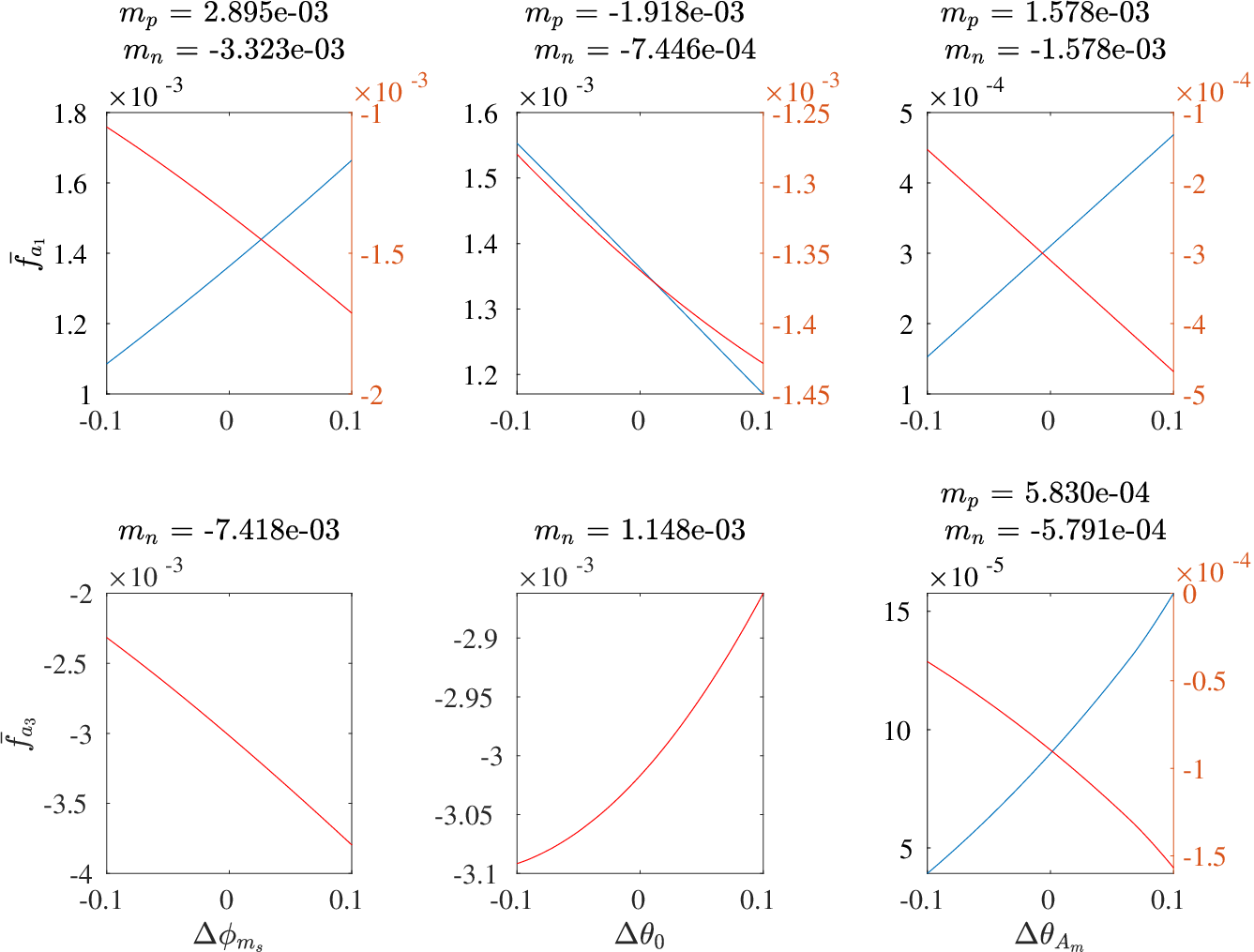
Employing these relations, we choose the wing kinematics parameters such that the variation of the averaged force $\Delta\bar{f}_{a}$ matches with a PID controller as follows.

where $K_{P},K_{D},K_{I}>0$ are the controller gains. After decomposing the longitudinal motion from the lateral motion, the wing kinematics parameters are computed from the following linear approximation. For the longitudinal forces, we have

where the matrix $S\in\mathbb{R}^{3\times 3}$ is defined as

When calculating $S$, the value of the sensitivity is chosen according to the sign of $\bar{f}_{a_{i}}$ as discussed above. For example, when $f_{a_{1}}>0$, we use $\dfrac{\partial\bar{f}_{a_{1}}}{\partial\phi_{m_{s}}}=\dfrac{\partial\bar{f}_{a_{1,p}}}{\partial\phi_{m_{s}}}$. As (27) is underdetermined, the control parameters are obtained by the minimum norm solution as

For a comparison, we consider another case when the abdomen is not actively controlled, i.e., $\Delta\theta_{A_{m}}=0$. The corresponding active control parameters $\Delta\phi_{m_{s}},\Delta\theta_{0}$ are computed by inverting the square matrix composed of the first two columns of (28). These ensure that the resultant aerodynamic forces in the longitudinal plane match with (26).

Next, for the lateral force,

In this subsection, we present simulation results with active abdomen control. The controller gains are chosen as $K_{P}=421.88,K_{D}=15.60,K_{I}=1.26$. Corresponding roots of the characteristic equation $\lambda^{3}+K_{D}\lambda^{2}+K_{P}\lambda+K_{I}$ are $-7.8+19i,-7.8-19i,-0.003$. Figure 5 illustrates the position and the velocity trajectory over the controlled dynamics starting from a perturbed initial condition, and it is shown that the states asymptotically converge to the desired periodic orbit.

Next, we verify the stability of the periodic orbit of the controlled dynamics via Floquet theory. Define an additional state $\delta I_{x}\in\mathbb{R}^{3}$ for the integral term as $\delta I_{x}=\int_{0}^{t}\delta x(\tau)d\tau$. And, the controlled dynamics of (12), where $Q_{i},\Omega_{i}$ are dependent of $\delta x$ and $\delta\dot{x}$, are numerically linearized. This yields the system matrix $\mathbf{A}(t)\in\mathbb{R}^{9\times 9}$ in (22), from which the monodromy matrix is computed. The corresponding characteristic multipliers are complex numbers with the following magnitudes:

Since the magnitude of all of the characteristic multipliers is less than or equal 1, the periodic orbit for the proposed controlled dynamics is stable. Moreover, the characteristic modes for the first three with $\rho=1$ predominantly consist of the integral term. Next, the modes with $|\rho|=\left\{0.1186,0.2835\right\}$ correspond to the longitudinal dynamics and they are much smaller than those of uncontrolled ones, namely $|\rho|=\left\{0.3763,0.6234\right\}$ in (24), thereby illustrating an improvement in stability. Finally, $|\rho|=\left\{0.6326\right\}$ corresponding to the lateral mode is greater than $\rho=\left\{0.5023\right\}$ of (24). However, it guarantees asymptotic stability of both of the position and the velocity dynamics.

Finally, we study the effects of the abdomen in the stability of the controlled dynamics. We consider two cases depending on the abdomen is actively controlled or not, and for each case we estimate the region of attraction with respect to the initial position error in the longitudinal plane. More specifically, we select $10,000$ random initial position errors of the form $\delta x(0)=[e_{x},0,e_{z}]$, where $(e_{x},e_{z})$ are sampled from the uniform distribution on the circle represented by $\{(r\cos{\theta},r\sin{\theta})\ |\ (r,\theta)\in(0,3)\times(0,2\pi)\}$. Each random initial point is propagated through the controlled dynamics, and it is determined to be converged if the position and the velocity error from the desired periodic orbit becomes less than $1\text{\times}{10}^{-4}$ within 100 periods. Figure 6 represents the set of initial conditions from which the controlled trajectory converged, and it is illustrated that the active abdomen undulation increases the region of attraction substantially.

Next, for the initial conditions that yield convergence for both cases, we compare the rate of convergence. It is observed that the number of flapping cycles required for convergence is smaller when the abdomen is actively controlled. The corresponding reduction of the flapping cycles cased by active abdomen control is illustrated at Figure 7, with respect to the varying magnitude of the initial error. For a wide variety of perturbations, it is found that there is a significant reduction.

In summary, the abdomen undulation can be actively controlled to improve the controller performance both by enlarging the region of attraction and by improving the rate of convergence.

References

- [1] M. Sun, J. Wang, and Y. Xiong, “Dynamic flight stability of hovering insects,” Acta Mechanica Sinica, vol. 23, no. 3, pp. 231–246, 2007.
- [2] H. E. Taha, M. R. Hajj, and A. H. Nayfeh, “Flight dynamics and control of flapping-wing mavs: a review,” Nonlinear Dynamics, vol. 70, no. 2, pp. 907–939, 2012.
- [3] M. Sun, “Insect flight dynamics: stability and control,” Reviews of Modern Physics, vol. 86, no. 2, p. 615, 2014.
- [4] D. B. Doman, M. W. Oppenheimer, and D. O. Sigthorsson, “Wingbeat shape modulation for flapping-wing micro-air-vehicle control during hover,” Journal of guidance, control, and dynamics, vol. 33, no. 3, pp. 724–739, 2010.
- [5] Z. A. Khan and S. K. Agrawal, “Control of longitudinal flight dynamics of a flapping-wing micro air vehicle using time-averaged model and differential flatness based controller,” in 2007 American Control Conference, pp. 5284–5289, IEEE, 2007.
- [6] W. He, Z. Yan, C. Sun, and Y. Chen, “Adaptive neural network control of a flapping wing micro aerial vehicle with disturbance observer,” IEEE transactions on cybernetics, vol. 47, no. 10, pp. 3452–3465, 2017.
- [7] J. Lee, S. Ryu, T. Kim, W. Kim, and H. J. Kim, “Learning-based path tracking control of a flapping-wing micro air vehicle,” in 2018 IEEE/RSJ International Conference on Intelligent Robots and Systems (IROS), pp. 7096–7102, IEEE, 2018.
- [8] M. Sridhar, C.-K. Kang, and D. B. Landrum, “Beneficial effect of the coupled wing-body dynamics on power consumption in butterflies,” in AIAA Scitech 2019 Forum, p. 0566, 2019.
- [9] J. Jayakumar, K. Senda, and N. Yokoyama, “Control of pitch attitude by abdomen during forward flight of two-dimensional butterfly,” Journal of Aircraft, vol. 55, no. 6, pp. 2327–2337, 2018.
- [10] J. P. Dyhr, K. A. Morgansen, T. L. Daniel, and N. J. Cowan, “Flexible strategies for flight control: an active role for the abdomen,” Journal of Experimental Biology, vol. 216, no. 9, pp. 1523–1536, 2013.
- [11] M. Sridhar, C.-K. Kang, and T. Lee, “Geometric formulation for the dynamics of monarch butterfly with the effects of abdomen undulation,” in AIAA Scitech 2020 Forum, p. 1962, 2020.
- [12] G. J. Berman and Z. J. Wang, “Energy-minimizing kinematics in hovering insect flight,” Journal of Fluid Mechanics, vol. 582, pp. 153–168, 2007.
- [13] C. P. Ellington, “The aerodynamics of hovering insect flight. i. the quasi-steady analysis,” Philosophical Transactions of the Royal Society of London. B, Biological Sciences, vol. 305, no. 1122, pp. 1–15, 1984.
- [14] T. Lee, M. Leok, and N. McClamroch, Global Formulation of Lagrangian and Hamiltonian Dynamics on Manifolds. Springer, 2018.
- [15] M. H. Dickinson, F.-O. Lehmann, and S. P. Sane, “Wing rotation and the aerodynamic basis of insect flight,” Science, vol. 284, no. 5422, pp. 1954–1960, 1999.
- [16] S. P. Sane and M. H. Dickinson, “The control of flight force by a flapping wing: lift and drag production,” Journal of experimental biology, vol. 204, no. 15, pp. 2607–2626, 2001.
- [17] G. Teschl, Ordinary differential equations and dynamical systems, vol. 140. American Mathematical Soc., 2012.