Solving the electron and muon anomalies in modelsPreprint: ULB-TH/21-01
Abstract
We consider simultaneous explanations of the electron and muon anomalies through a single of a extension to the Standard Model (SM). We first perform a model-independent analysis of the viable flavour-dependent couplings to leptons, which are subject to various strict experimental constraints. We show that only a narrow region of parameter space with an MeV-scale can account for the two anomalies. Following the conclusions of this analysis, we then explore the ability of different classes of models to realise these couplings, including the SM, the -Higgs Doublet Model, and a Froggatt-Nielsen style scenario. In each case, the necessary combination of couplings cannot be obtained, owing to additional relations between the couplings to charged leptons and neutrinos induced by the gauge structure, and to the stringency of neutrino scattering bounds. Hence, we conclude that no extension can resolve both anomalies unless other new fields are also introduced. While most of our study assumes the Caesium measurement, our findings in fact also hold in the case of the Rubidium measurement, despite the tension between the two.
I Introduction
The excellent agreement between the Standard Model (SM) and experimental observations makes the persisting anomalies all the more interesting. One long-standing discrepancy between theory and experiment is that of the anomalous magnetic dipole moment of the muon, , which has recently been updated to a tension with the SM Bennett:2006fi; Aoyama:2020ynm; Abi:2021gix11 1 We note that the significance of this anomaly has been questioned by a lattice QCD calculation of the leading-order hadronic vacuum polarisation contribution to Borsanyi:2020mff. ,
| (1) |
Further data from the ongoing Muon g-2 experiment at Fermilab is expected to reduce the uncertainty by a factor of four Grange:2015fou, and the future J-PARC experiment forecasts similar precision Abe:2019thb, both of which should clarify the status of this disagreement. To add to the puzzle, an anomaly emerged in the electron sector due to a) an improved measurement of fine-structure constant, , using Caesium atoms Parker:2018vye, from which the value of may be extracted, and b) an updated theoretical calculation Aoyama:2017uqe. This yielded a discrepancy in the electron anomalous magnetic moment of
| (2) |
which constitutes a tension with the SM Davoudiasl:2018fbb. Notably, this has the opposite sign to the muon anomaly, Eq. (1). Recently, however, a new measurement of the fine-structure constant using Rubidium atoms gave Morel:2020dww
| (3) |
This is a milder anomaly, the discrepancy between experiment and SM being only 1.6, and it is in the same direction as the muon anomaly. Remarkably, the Caesium and Rubidium measurements of disagree by more than , therefore it is difficult to obtain a consistent picture of .
Given this uncertain status quo, in this paper we choose to focus predominantly on the earlier Caesium result, Eq. (2), and only discuss the Rubidium result in section V (which, however, is the first analysis of this new experimental situation, to the best of our knowledge). The presence of dual anomalies in the electron and muon sectors motivates an exploration of new physics models that could simultaneously explain both. Moreover, the relative size and sign of these anomalies poses an interesting theoretical challenge.
Let us consider these issues. Firstly, the opposite signs of and (from now on we will drop the superscript) immediately excludes all new physics models whose contribution to the magnetic dipole moment of charged leptons has a fixed sign. The dark photon Holdom:1985ag, for instance, generates , and therefore cannot satisfy the dual anomalies. Secondly, the contribution from flavour-universal new physics to is generally expected to be proportional to the mass or mass squared of the lepton (see e.g. Freitas:2014pua; Dorsner:2016wpm), whereas from Eqs. (1) and (2) we find
| (4) |
These considerations, along with numerous low scale constraints discussed below, lead to significant model-building obstacles. So far, various attempts have been made to explain the anomalies, with different solutions relying on the introduction of new scalars, SUSY, leptoquarks, vector-like fermions, or other BSM mechanisms, see e.g. Crivellin:2018qmi; Endo:2019bcj; Badziak:2019gaf; Hiller:2019mou; Bauer:2019gfk; Endo:2020mev; Giudice:2012ms; Davoudiasl:2018fbb; Liu:2018xkx; Dutta:2018fge; Gardner:2019mcl; Cornella:2019uxs; Dutta:2020scq; Yang:2020bmh; Crivellin:2019mvj; Bigaran:2020jil; Dorsner:2020aaz; Botella:2020xzf; Jana:2020pxx; Han:2018znu; Abdullah:2019ofw; CarcamoHernandez:2020pxw; Haba:2020gkr; Calibbi:2020emz; Arbelaez:2020rbq; Chen:2020jvl; Hati:2020fzp; Jana:2020joi; Chen:2020tfr; Chun:2020uzw; Li:2020dbg; Banerjee:2020zvi; Hernandez:2021tii; Darme:2020sjf. In this paper, we study a rather unexplored possibility that a (light) boson with flavour-dependent lepton couplings accounts for both anomalies.
A new gauge boson of a symmetry is a well-motivated candidate for many BSM models. It has long been considered a possible explanation of the anomaly Pospelov:2008zw (see also e.g. Davoudiasl:2014kua; 1511.07447; 1712.09360; 1901.09552; 1906.11297), thus it seems important to investigate if a extension of the SM can at the same time also resolve the anomaly. One immediate advantage of models is that it is possible to generate positive or negative contributions to the magnetic moment simply by adjusting the relative size of its vector and axial couplings to fermions, as will be shown below.
We focus on the in mass range , which is a natural consequence of various experimental bounds (more on this in Sections II.2 and III). A in the MeV mass range has been of interest (see e.g. Feng:2016ysn; Kozaczuk:2016nma; Lindner:2018kjo; Bauer:2018onh; DelleRose:2018eic; Smolkovic:2019jow) due to hints of a new MeV boson to explain anomalies in nuclear transitions observed by the Atomki collaboration, both in Beryllium Krasznahorkay:2015iga, and more recently Helium Krasznahorkay:2019lyl. Models with MeV-scale also have the capacity to generate in the early Universe Escudero:2019gzq, thereby somewhat ameliorating the Hubble tension Bernal:2016gxb. The question then is whether the scenario survives the wealth of sensitive experiments, in particular for . To answer this, we first perform a model-independent analysis to identify regions in the parameter space of models that can successfully explain both the anomalies. This to our knowledge is the first study of this scenario in such a general and model-independent way, although a specific model was previously studied in the context of the dual anomalies and found not to work CarcamoHernandez:2019ydc. Note that we are focusing on the minimal scenario where the additional contribution to the anomalous magnetic moments comes solely from the , which is different from some of the other models studied in literature that include a plus other new fields (e.q. Hati:2020fzp; Banerjee:2020zvi; CarcamoHernandez:2019ydc). The conclusions from our model-independent analysis serve as a powerful tool in checking the viability of various specific models, and we hope that it will be useful for more complex model-building.
The layout is as follows: Section II introduces our conventions for the effective couplings and potential origins of these couplings. We study experimental constraints on these couplings in Section III, summarising our findings in Figs. 2 and 3. In light of the array of experiments probing light vector bosons in the near future, we discuss the discovery potential of such a in Section III.3. Equipped with the model-independent analysis, in Section IV we consider several models and the challenges they face. We demonstrate that some of the simplest and most common classes of extensions of the SM cannot explain the two anomalies simultaneously. Finally, in Section V we address the Rubidium anomaly and study the capacity of a model to explain it in conjunction with the anomaly.
II Formalism of a light
II.1 Effective couplings
In the most general framework, a new with family-dependent charged lepton couplings leads to flavour violation. However, in this paper we assume that the charged lepton Yukawa matrix and the matrix of charged lepton couplings are simultaneously diagonalisable and therefore the has only lepton-flavour conserving couplings. Various flavour models predict such scenarios (see, for instance, Criado:2019tzk) and in this way we avoid stringent limits on flavour-violation, such as from TheMEG:2016wtm. Flavour-conserving couplings of fermions to the can be described through , with gauge current,
| (5) |
Rewriting the charged lepton interactions in terms of vector and axial couplings, , gives
| (6) |
It is typically a simple exercise to derive these effective couplings for a given model. For now we assume that the different effective couplings are unrelated. In models with no extra fermions, there are three different contributions to the couplings of SM fermions to the arising from a gauge group. These are:
- •
Charge assignment of the fermion under the (flavour dependent).
- •
Gauge-Kinetic Mixing (GKM) arising from the Lagrangian term , where and are the field strength tensors of hypercharge and , respectively (flavour universal).
- •
mass mixing, which is generated if the SM Higgs sector is charged under the (flavour universal).
The combination of these three contributions can generate variety of vector and axial couplings. As explained in the introduction, in this work we are concerned with exploring the possibility that a single accounts for the discrepancies. We will firstly survey the parameter space in a model-independent way in terms of the effective lepton- couplings defined in Eq. (6). The conclusions from this analysis are then used in Sections IV and V to study whether these couplings can be realised in a few specific classes of models.

II.2 Contribution to the charged lepton anomalous magnetic moment
The modifies the magnetic moment of a charged lepton via the one-loop diagram in Fig. 1. In the notation of Eq. (6), the contribution for a charged lepton of flavour is Leveille:1977rc
| (7) |
In the limits and , this simplifies to
| (8) |
We see that the way to achieve correct signs for the contributions to muon and electron anomalies ( and ) is with a non-zero axial coupling for the electron () and vector coupling for the muon ().
We remark that it is impossible to satisfy both the anomalies simultaneously if we demand flavour universality, i.e. and . This is straightforward to see from Eq. (8) when or . For the remaining case of , solving the anomalies demands and , which is inconsistent with flavour universality.22 2 It is interesting to note that if the anomalies had the opposite sign, i.e. had the experimental data required and , then and could have given a viable solution. Thus, neither the different sign nor the unusual ratio of the anomalies necessarily implies that flavour non-universal physics must be present. This is precisely why we consider models with flavour-dependent couplings in this paper.
We may now make some broad arguments about preferred values. In the case of a light with , even the smallest effective couplings required to explain the anomalies, accomplished by setting , lead to orders of magnitude between and , which could only be accounted for by either an orders of magnitude difference in their charges under the or a very fine-tuned cancellation of the flavour-dependent part of against the flavour-universal contribution. We will see in Section III that such a light with couplings sufficiently large that it satisfies the anomalies is in any case excluded by cosmological constraints. Therefore, we will focus on .
For the heavy regime, i.e. , two arguments follow. Firstly, considering the muon sector, in the region , the new vector boson is excluded by BaBar from its decay into two muons BaBar:2016sci, while for GeV GeV it is similarly excluded by CMS CMS:2018yxg. Turning to the electron sector, we note that for GeV, the axial coupling to electrons required to satisfy the anomaly in electron sector is . With such large couplings to electrons, any GeV-scale object would have likely showed a signal at previous colliders, such as SLAC RF linac, LEP and LHC runs. A heavy solution to the anomalies therefore seems improbable given these considerations. Finally, in the intermediate range, , the values of and required to explain the two anomalies are of a similar order of magnitude, which lends this mass range to potentially more natural, i.e. less fine-tuned, solutions and so we will focus on this regime in the remainder of this paper.
III Model-independent analysis of Constraints on couplings
The effective couplings introduced in Eq. (6) are subject to a wide variety of constraints, which we shall now discuss. In general, the could couple to all SM fermions, and indeed there are some rather stringent bounds on couplings to quarks. However, we will focus on interactions with electrons and muons, those being the critical ones for the explanation of the anomalies. Since lepton doublets contain both charged leptons and neutrinos, non-zero effective couplings to charged leptons generally imply effective couplings to neutrinos, which have their own experimental constraints. This will be borne out in the example models considered in Section IV.33 3 The dark photon is a notable counter-example, with interactions solely generated through gauge-kinetic mixing, where while . However, the dark photon does not successfully explain the anomalies because, as is easily seen from Eq. (7), implies .
For a given explicit model, there may be many additional constraints. These can arise in several different ways. Firstly, as mentioned just above, the may also couple to the tau or to quarks. Bounds on couplings to light quarks are discussed for instance in Feng:2016ysn; Kozaczuk:2016nma; Bauer:2018onh; DelleRose:2018eic; Smolkovic:2019jow. Secondly, mixing leads to a shift in boson couplings, which have been very precisely measured at LEP ALEPH:2005ab, as well as other electroweak-scale parameters.
While there may be such model-dependent bounds, the goal of this section is to study the viability or otherwise of a solution to the two anomalies based on leptonic couplings alone. The plethora of experimental constraints are described below, with our results summarised in Figs. 2 and 3.
III.1 Couplings to electrons
We first outline the most important limits on the effective couplings of the to electrons (, ) and electron neutrinos ().
III.1.1 Cosmological and astrophysical bounds
MeV-scale states with even very small interactions with electrons or neutrinos (effective couplings as tiny as ) can remain in thermal contact with the SM plasma during Big Bang Nucleosynthesis (BBN) and thereby significantly alter early universe cosmology. Bounds on the masses of electrophilic and neutrinophilic vector bosons from various cosmological probes were calculated in Sabti:2019mhn. Combining BBN and Planck data, they found at 95.4% C.L. that an electrophilic , i.e. , is constrained to have a mass of at least 9.8 MeV. From Eqs. (2) and (8), we see that for MeV, the effective electron- coupling should be , so the BBN bounds do apply here. The limit is slightly weakened for larger , therefore we take MeV as a conservative lower bound on our mass.44 4 This bound can in principle be avoided by sufficiently light . When eV, the anomaly can be explained with . However, we will see in Sec. III.2 that such a light solution to the discrepancy is ruled out by similar cosmological considerations.
The also affects various aspects of stellar evolution. The most critical of these for a MeV-scale is white dwarf cooling Dreiner:2013tja. The mediates an additional source of cooling, via . Since the mass under consideration is much larger than white dwarf temperatures, keV, this can be treated as an effective four-fermion interaction at the scale with the integrated out. Motivated by the good agreement between predictions and observations of white dwarf cooling, the benchmark set by Dreiner:2013tja is that new sources of cooling should not exceed SM ones. We therefore impose
| (9) |
as an approximate bound. When plotting this constraint in Fig. 2, we assume that only , and are non-zero.
Finally, we note that a which couples to neutrinos can also be an additional source of energy loss for supernovae, if it is able to escape the supernova core. We followed the formalism in Appendix B of Escudero:2019gzq and enforced that the additional energy loss due to the is no greater than the energy loss in the SM during the first ten seconds of the supernova explosion. However, for a roughly MeV-scale this observation only constrains a band of effective couplings , which is much too small to be relevant for the anomalies.
III.1.2 Collider and beam dump bounds
A stringent limit on interactions with electrons comes from the BaBar experiment, which searched for a dark photon, , via with . The results are reported in Lees:2014xha and probe masses from 20 MeV up to 10.2 GeV. The bound on , the kinetic mixing parameter in the dark photon model arising from the gauge-kinetic term can be converted into a limit on . We neglect the statistical fluctuations in the BaBar bound (cf. Fig. 4 of Lees:2014xha), opting conservatively to extrapolate from the most constraining points of the 90% confidence exclusion region and obtain our bound by interpolating between these. This constraint becomes mildly stronger with mass, with for instance
| (10) |
for MeV. For , the is sufficiently light that it decays only to electrons and neutrinos. We will see that the couplings to electrons should generically be much larger than couplings to neutrinos, thus .
The BaBar result alone rules out a vast region of parameter space. The smallest axial coupling required to satisfy the discrepancy is given by , as can be seen from Eq. (8) by setting . Then the BaBar bound for MeV rules out all solutions (notwithstanding some statistical fluctuations) with a heavier than 40 MeV up to the largest mass probed by the experiment, 10.2 GeV. This limit only strengthens for , since a larger is then required to explain , while at the same time is more constrained because BaBar bounds the combination .
The KLOE experiment also constrains the coupling to electrons Anastasi:2015qla. Although generally weaker than BaBar’s limit, its exclusion region covers additional parameter space since the experiment probes masses as small as 5 MeV. For these low masses, the bound is around
| (11) |
Beam dump experiments probe the couplings to electrons, since the may be produced and detected via , see e.g. Bjorken:2009mm. The produced s should therefore decay in the dump before they reach the detector. The best bound comes from NA64 Banerjee:2019hmi, which sets limits on a with masses between 1 MeV and 24 MeV.
A further stringent bound on the parameter space comes from the precise measurement of parity-violating Møller scattering at SLAC Anthony:2005pm. For masses below around 100 MeV, the bound is independent of and yields Kahn:2016vjr
| (12) |
As indicated above, a tiny is ideal for explaining the anomaly while avoiding collider constraints with as small a value of as possible. Taking close to zero is clearly also an efficient way to evade this Møller scattering limit.
III.1.3 Neutrino scattering bounds
Very strong restrictions on the effective couplings come from measurements of neutrino-charged lepton scattering Lindner:2018kjo. There have been many experiments testing neutrino interactions. Here we study the most relevant ones: TEXONO Deniz:2009mu Borexino Bellini:2011rx, and CHARM-II Vilain:1993kd. These experiments are known to be among the most constraining in general (see e.g. Feng:2016ysn; Lindner:2018kjo; Bauer:2018onh; Smolkovic:2019jow), they cover a range of energies and different neutrino flavours. Let us first consider TEXONO. The typical energy transfer in a scattering event is , where MeV is the electron recoil energy. With MeV (as enforced by the limits from cosmology), we may safely make the assumption . The correction to the SM cross-section of anti-neutrino scattering is then
| (13) |
following Ref. Lindner:2018kjo. Comparing this with the TEXONO measurement, Deniz:2009mu puts extremely stringent bounds on the effective couplings.
Borexino measures the scattering of solar neutrinos. The electron neutrino survival probability is measured as , while the experiment cannot distinguish muon and tau neutrinos. For simplicity, we therefore assume that 50% of the scattered neutrinos are electron neutrinos, with 25% each of muon and tau neutrinos.55 5 This assumption has negligible bearing on our main results since is specifically probed by CHARM-II, as outlined below, and we are not concerned with . Then the scattering rate induced by the is
| (14) |
The cross-section including new physics should not deviate from the SM cross-section by more than about 10 Bellini:2011rx; Harnik:2012ni, and this restriction sets a strong limit on the parameter space. Note from Eqs. (13) and (14) that and can both be large as long as the are sufficiently small.


III.1.4 Analysis of constraints in the electron sector
We now combine all the constraints discussed above to analyse viable parameter space for the explanation of . Our results are summarised in Fig. 2. In the plots, effective couplings to muons and taus are set to zero, which is relevant for the bounds from White Dwarfs and Borexino, cf. Eqs. (9) and (14) respectively. We first set the neutrino coupling, , to zero in Figs. 2 (a,b) to analyse limits solely on the electron couplings, and plot constraints on the axial electron coupling, , against the vector boson mass, . We focus on the axial coupling for two reasons. Firstly, generates the required by experiment. Secondly, axial couplings provide various model-building challenges, see Section IV.
For each value of and , in Figs. 2 (a,b) we choose such that the loop induces a correction to that is respectively less than and greater than the discrepancy of Eq. (2), i.e. in Fig. 2 (a) and in Fig. 2 (b). This therefore displays the full range of masses and axial couplings which can reduce the anomaly to less than . Note that the signs of and are irrelevant for Figs. 2 (a,b) since all constraints in these plots bound only their absolute values. The blue triangular regions in the lower right half of Figs. 2 (a,b) correspond to values of and such that it is impossible to generate the desired deviation in , regardless of the value of . The other shaded regions are excluded by the experimental constraints discussed above. In both plots there is a thin white strip, bounded between the blue and yellow Møller exclusion regions, which represents the allowed parameter space. The smallness of these allowed regions shows that even before any model-building considerations are taken into account, it is rather difficult to satisfy the anomaly while obeying the copious experimental constraints we have mentioned. In the white strips, . Indeed, since the parity-violating Møller scattering bound is , we find that since is needed to explain the anomalies, we therefore have . As the vector coupling of to electron is required to be smaller than the axial coupling, Eq. 8 for electron is well approximated by
| (15) |
Following this conclusion, we set in Figs. 2 (c,d) to explore the maximum allowed parameter space for the neutrino coupling, , against the mass . Similar to before, in the left plot, Fig. 2 (c), we set such that is below its experimental value, while in the right plot, Fig. 2 (d), we set to above it. These values of can be taken from Eq. (15). We take here: if instead , Figs. 2 (c,d) look the same but reflected about the -axis, since all bounds are invariant under and when . The Texono and White Dwarf bounds become apparent in these two plots, however we note that both Møller scattering and KLOE constraints are satisfied when and therefore do not appear. A key conclusion from Figs. 2 (c,d) is that NA64 and BaBar effectively restrict the mass range of a which can satisfy the anomaly to within to be . In both cases, Borexino gives the strongest constraint on neutrino coupling, , more than an order of magnitude smaller than the required axial coupling.
In summary, it is clear that a solution to just the anomaly alone requires some specific ingredients. In particular, should be larger than and at least an order of magnitude larger than , while the mass of is constrained to a small window MeV MeV.
III.2 Couplings to muons
Now we turn to the bounds on the effective couplings of the to muons and the muon neutrino, namely , , and . There are fewer bounds on these than on the couplings to electrons for a few reasons. One is that electrons, being stable, are far easier to handle experimentally. Another reason is that we are led to probe masses sufficiently light that they don’t decay into muons. Then, as we have seen, various experiments constrain from the absence of but cannot similarly constrain from the absence of the decays as these are already kinematically forbidden. Despite this, there remain various strict limits on interactions with muons and muon neutrinos.
III.2.1 Cosmological and astrophysical bounds
When , bounds from BBN and Planck studied by Sabti:2019mhn set a lower limit on the mass, MeV. This is similar to the limit on new electrophilic species outlined at the start of Section III.1. For , however, it may seem that lower masses are in principle allowed. For a light (), a minimum vector coupling to muons of is required to reduce the tension to within . This coupling ensures that the was in thermal equilibrium with the SM at earlier times. After decoupling (at temperature ), a very light would constitute an extra relativistic species contributing to the expansion rate of the Universe during neutrino decoupling and BBN, which took place between . In general, we therefore consider MeV to avoid constraints from measurements of and primordial element abundances.
Additionally, we note that a study of energy loss in supernovae due to interactions by Croon:2020lrf rules out a with coupling for masses less than eV.66 6 In the models studied in Croon:2020lrf, the has interactions with both muons and muon neutrinos. However, at low masses MeV) it is the interactions with dominate the bounds, while the interaction plays a negligible role. Recall, however, that for eV, the effective coupling required to explain the anomaly must be greater than . With an interaction of this size, the BBN bound on a new electrophilic species dictates that must be at least in the MeV range.
We can therefore rule out the possibility of an extremely light (i.e. MeV) being able to explain the two anomalies. Its mass must consequently be at least 16 MeV, as we showed from the analysis of constraints on couplings to the electron sector in the previous section.
III.2.2 Neutrino scattering bounds
Several neutrino scattering experiments bound couplings to muons and muon neutrinos. The most stringent of these are Borexino and CHARM-II, introduced above. The Borexino result was given in Eq. (14). The mean (anti)neutrino energy in the CHARM-II experiment is much larger than the masses we consider, with GeV and GeV Vilain:1993kd, therefore the approximation which we used to obtain Eqs. (13) and (14) cannot be used. We apply the formalism in Harnik:2012ni; Lindner:2018kjo to obtain numerical results, which enter into Fig. 3 by enforcing that the shift in the neutrino scattering cross-section induced by the is no greater than Lindner:2018kjo. We mention that some doubts on the CHARM-II analysis were presented in Bauer:2018onh, however we do not enter into this discussion.
A with couplings to muons and muon neutrinos also modifies the neutrino trident process, Altmannshofer:2014pba. Neglecting the coupling , since is necessary to explain the anomaly when (see Eq. (8)), the trident cross-section including the contribution is Altmannshofer:2014pba
| (16) |
This can be compared with the CCFR measurement, Mishra:1991bv, to give a constraint.


III.2.3 Analysis of constraints in the muon sector
We combine the results of the above constraints in Fig. 3. In Fig. 3 (a) we plot the allowed regions for the effective vector coupling of the to the muon, , against the mass, with relevant constraints overlaid, while setting and fixing such that is satisfied. The large white-space shows the parameter space which can explain the anomaly and is not excluded. It reflects the fact that when a light couples only to muons, there are few relevant constraints. can be as large as in the mass region of interest, MeV MeV. In purple on the left of Fig. 3 (a), (c) and (d) is the mass bound MeV from BBN and Planck data. The pink bounds at the top and bottom of (a) come from the CCFR neutrino trident measurement, see Eq. (16). The thin blue line for gives the region for which is too small to reduce the tension to within , even if . Then (b) shows contours of the necessary values of to exactly satisfy the anomaly, given and . This can be as large as , but must always be at least factor of a few smaller than .
The bounds on the interaction with muon neutrinos are significantly stronger. Fig. 3 (c) and (d) show bounds on neutrino couplings from various experiments (we take ). We must invoke couplings to electrons, since modifications to both neutrino scattering on electrons and white dwarf cooling necessarily depend on the coupling to electrons, as does detection at beam dumps. To be as minimal as possible, we take only non-zero , assuming . In (c) is set (as a function of ) such that is below its experimental value, while in (d) it is set such that is instead above. This allows us to see the full range of allowed . Clearly, its absolute value cannot be much larger than , which justifies the choice of in plot (a). Taking instead would only flip (c) and (d) about the -axis, since the neutrino scattering and white dwarf constraints are invariant under and when those are the only non-zero couplings.
III.3 Future Discovery Potential
Having surveyed the current limits, in this section we will discuss future experiments which could discover (or preclude) the low scale explanation of by closing the allowed parameter space given in Figs. 2 and 3 (keeping in mind that these were generated assuming the Caesium result). The place to start is with the magnetic dipole moment anomalies themselves. The two highly inconsistent measurements of (from which the value of is derived) made in Caesium Parker:2018vye and Rubidium Morel:2020dww atoms demand a third independent experiment to resolve the situation. It is indeed not even clear whether an anomaly exists. On top of this, the Muon g-2 and J-PARC experiments Grange:2015fou; Abe:2019thb are expected to provide improved measurements of , which is particularly important given the recent debate about the SM prediction Borsanyi:2020mff. Beyond this, there are several future experiments which are expected to test the allowed couplings to charged leptons.
We note first of all that an improved measurement of parity-violating Møller scattering can never close the parameter space, as this bounds the combination , which can always be satisfied by taking one of or to zero while the other (depending on the sign of the anomaly) explains the discrepancy. Thus, we will not discuss future experiments in this area.
To fully probe the available space, we require other bounds to be strengthened. Currently, the lower bound on the mass, MeV, is fixed from NA64’s visible decay limits. Future NA64 results after the LHC’s Long Shutdown 2 (LS2) should probe masses up to around 20 MeV 2003.07257.
For higher masses, the most sensitive future experiment will be Belle-II 1808.10567, from the visible dark photon search mode . With 50 ab-1 luminosity (expected in 2025), the projected sensitivity is Ferber:2015jzj
| (17) |
An alternative experiment with similar sensitivity is MAGIX at MESA 1809.07168, which is also currently under construction and expecting results in the next few years. The combination of NA64 and Belle-II (or MAGIX) could entirely rule out or discover low scale explanations of the current Caesium result. Beam dumps (e.g. FASER 1811.12522 and SHiP 1504.04855) are also expected to play a role. This provides hope that a firm conclusion could be reached within the next few years.
The MUonE experiment Banerjee:2020tdt will probe the product of couplings to electrons and to muons. In this way it is a unique test of a which explains both anomalies, because it is required to have significant couplings to both leptons. The experiment is expected to cover a significant portion of the parameter space which remains open, see Dev:2020drf; Masiero:2020vxk.
Finally, we point out that while there are many dark photon experiments beyond those listed above, many do not directly test our framework. There are two reasons for this. Firstly, we are concerned with the lepton- couplings only, so experiments which involve production of the though quarks are not applicable. This includes electron-proton scattering (such as DarkLight 1412.4717), proton-proton scattering and pion decays (e.g. NA62 CortinaGil:2019nuo). Secondly, we require visible () decays of the , which excludes the invisible-only experiments such as PADME KozhuharovonbehalfofthePADMECollaboration:2018exf, VEPP-3 Wojtsekhowski:2017ijn, BDX Battaglieri:2019nok and LDMX 1808.05219. Consequently, the available parameter space in Figs. 2 and 3, and hence the discovery potential, may only be fully reached by the small number of experiments which focus on vector bosons produced by leptons and which decay to .
IV Viability of specific models
Having completed our model-independent analysis in Section III, we now turn to specific realisations of models. The ingredients for the simultaneous explanation of the anomalies with a single are:
- 1.
A light in the mass range .
- 2.
Axial coupling of the to electrons larger than the vector coupling: .
- 3.
Large vector coupling to muons, , and an axial coupling that is smaller by at least a factor of a few.
- 4.
Tiny couplings to neutrinos: .
We now attempt to realise this hierarchy of couplings in various classes of models, each of which inevitably introduces additional relations between effective couplings. We will begin with the simplest case of just the SM extended by a . We will then move onto a scenario with additional Higgs doublets, and finally discuss the viability of a Froggatt-Nielsen style model, in which the gauge invariance of the charged lepton Yukawa interactions is relaxed. Note that in each case the dominant contribution to the shift in comes solely from the .
Before commencing, we also remark that the cancellation of gauge anomalies is crucial for constructing a consistent theory. The and anomalies can always be satisfied by introducing additional chiral fermions which are charged under the but sterile with respect to the SM (in fact one needs at most five Allanach:2019uuu). The anomaly cancellation conditions involving SM groups are typically more challenging to satisfy. However, this section addresses the primary question of whether it is possible to generate the desired effective couplings, without delving into how to do so in an anomaly-free way.
IV.1 SM+
First consider a minimal model, in which the SM is extended by a gauge and also add a scalar, , charged under the , whose non-zero VEV, , spontaneously breaks the symmetry. We note here that this unspecified covers in particular the case of gauging combinations of electron, muon and tau number, i.e. for some . Let us establish the formalism, which will also be useful for the subsequent models.
In general there is mixing between and , and the kinetic terms for the pair of s can be written as
| (18) |
where is the gauge field associated with and is the corresponding field strength tensor.
An appropriate rotation and rescaling of fields removes the mixing (see e.g. Coriano:2015sea),
| (19) |
and leaves the couplings in the covariant derivative in the form,
| (20) |
where and are the respective and gauge couplings, and and are the respective charges of the field under and . In the above, we have only kept terms that are leading order in the kinetic mixing parameter , which is taken to be small. This gives . Breaking the EW and symmetries and diagonalising the gauge boson mass matrix, we move into the basis of mass eigenstates, , , and , using
| (21) |
where is the weak-mixing angle, is the mixing angle, and () denotes sine (cosine). This gauge boson mixing is given by
| (22) |
where , () is the charge of the Higgs . Finally, after outlining this procedure, we can write the effective couplings of SM fermions to the gauge boson mass eigenstates. We find that the effective couplings for charged leptons at leading order in are
| (23) | ||||
| (24) |
where () is the charge of the lepton doublet (singlet), ().
Here we see from the invariance of the SM charged lepton Yukawa couplings, , we have that . Consequently, at leading order in , and therefore . Under this condition, the with always induces a positive shift in , cf. Eq. (8), which is the wrong direction for explaining the Caesium anomaly. The simplest extension of the SM can therefore be ruled out as a possibility of resolving both and discrepancies.
IV.2 NHDM
We have seen that extending the SM by just a gauge and a scalar does not give us enough freedom to arrange . There are several options to circumvent this problem, including a) introducing new fermions which mix with the SM ones, b) extending the Higgs sector, or c) removing the gauge invariance of the Yukawas via a Froggatt-Nielsen Froggatt:1978nt type set-up. In the case of option (a), our analysis is not valid because loops involving the new fermions could also contribute to .77 7 An attempt to explain both anomalies by introducing a heavy vector-like fourth family of leptons was made in CarcamoHernandez:2019ydc but was ultimately unsuccessful. Here we consider option (b). This was previously explored e.g. in the context of the Atomki anomaly DelleRose:2017xil. In Section IV.3 we will consider option (c).
Let us take the type-I 2HDM, wherein all SM fermions couple to the same Higgs doublet, . This choice will not be important for the following discussion, since we are concerned only with the lepton couplings, thus our discussion is general. We can also generalise to the case of many Higgs doublets, see for instance Appendix A of Lindner:2018kjo. The key point is that this set-up modifies Eq. (24) and therefore permits non-negligible axial couplings.
The kinetic mixing between and and the subsequent modification of covariant derivatives is as described in Eqs. (18)-(20). The neutral gauge boson mass mixing is modified by the presence of two Higgs fields, , with charges and VEVs , where and . Then the mixing angle is given by
| (25) |
where
| (26) |
with for . Note that in the limit , i.e. when only () is non-zero, we recover the result of Eq. (22) up to . Accounting for the kinetic and mass mixing, the effective couplings for charged leptons and neutrinos at leading order in in are
| (27) | ||||
| (28) | ||||
| (29) |
using that the -invariance of the charged lepton Yukawa couplings demands . We see that can be non-zero when , and that it is flavour-universal. and , on the other hand, are flavour-dependent. However, both depend linearly on , so that
| (30) |
Consequently, there are not six independent effective couplings for , but rather only four are independent. Given this, it is in fact simple to argue that this class of models cannot simultaneously explain the anomalies. Our model-independent analysis in Section III established that due to the stringency of the bounds from neutrino scattering experiments, the effective neutrino couplings must be tiny: , cf. Figs. 2 and 3. From Eq. (30), this implies that we need . However, it is apparent from points 2 and 3 of the summary list at the beginning of this section that . Clearly, this framework is not successful.
In the simplest extension of the SM, only the anomaly could be resolved as it was impossible to generate significant axial couplings of the . Introducing additional Higgs fields enables large axial couplings, so that either the or the anomaly may be explained. However, the correlations between different effective couplings and the strength of the bounds on neutrino couplings conspire to preclude an explanation of both anomalies at the same time.
IV.3 Froggatt-Nielsen model
A second way to generate sizeable axial couplings, as is necessary to explain the Caesium anomaly, is by considering a Froggatt-Nielsen type model Froggatt:1978nt. In this set-up, we modify the charged lepton Yukawa interactions to some effective interactions of the form,
| (31) |
Here is a diagonal matrix of couplings (in the charged lepton mass basis), is a flavon, is a diagonal matrix whose entries are determined by the charges of the flavon and the SM leptons, and is the scale of some unspecified UV physics. Then the SM charged lepton Yukawa couplings are recovered at the non-zero VEV of the flavon, i.e. . More complicated set-ups can also be written down (e.g. the clockwork model of Smolkovic:2019jow), and there may be more than one flavon.
The introduction of flavons removes the relation between the charges of the SM leptons and the Higgs. This permits non-vanishing axial couplings at leading order in , unlike in the standard SM scenario, (recall Eq. (24)). From Eq. (31) we have , and we have the freedom to treat as a free, family-dependent parameter.88 8 In this framework we will not attempt to generate the observed charged lepton Yukawa couplings, but rather focus on whether the anomalies can be simultaneously explained In all other respects, the formalism of this model follows that of the extension outlined in Section IV.1. Eqs. (22)-(24) still hold, while the effective neutrino couplings are given by
| (32) |
at leading order in . This model was previously studied in DelleRose:2018eic to explain the Atomki Beryllium anomaly Krasznahorkay:2015iga, another instance in which unsuppressed is required.
Combining Eqs. (23), (24) and (32) gives
| (33) |
This is a generalisation of Eq. (30) to the case of non-universal . However, we see from Fig. 2 (a) and Eq. (7) that in order to reduce the anomalies to while satisfying all experimental constraints, we require and , given MeV, the lower bound on the mass obtained in Section III. However, we have established that , while the Møller scattering bound gives for . Finally, a sizeable demands an even larger , since to a good approximation, see Eqs. (7) and (8). Thus, , while in the mass range of interest, and hence there is no combination of effective couplings fulfilling Eq. (33) such that both anomalies are satisfied to within and all experimental constraints are satisfied. It is notable that even in such a general theoretical setting, the explanation is unsuccessful.
V solutions considering the Rubidium measurement
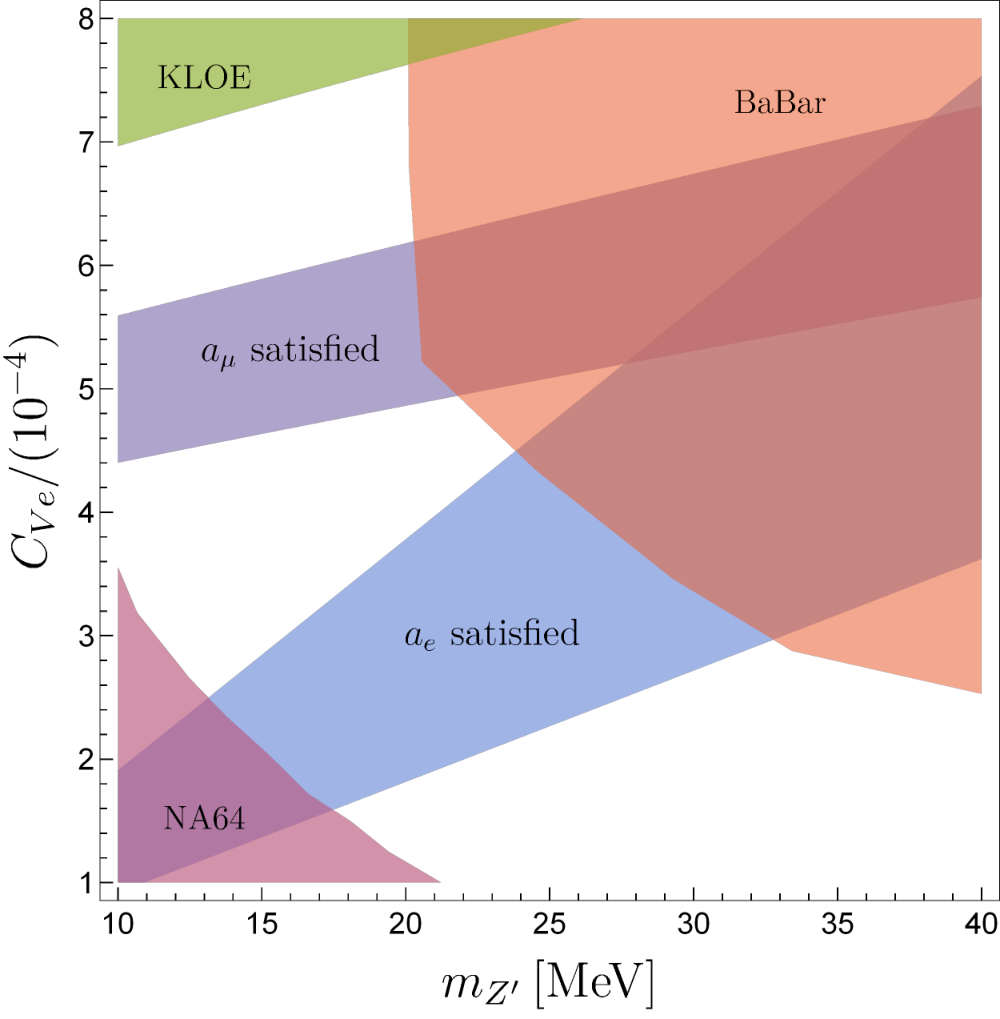
We have thus far considered only the anomaly from the Caesium measurement, Eq. (2). Significantly, this has the opposite sign to the muon anomaly. In Section IV, it was shown that the combination of the different signs and sizes of the anomalies, along with the copious experimental constraints, makes it impossible to construct a model which can satisfy both at the same time. One might suppose that it is easier to explain two anomalies which have the same sign, which is exactly the situation if one considers instead the recent Rubidium result for , cf. Eq. (3). Here we consider this possibility. This has not, to the best of our knowledge, previously been studied. Our model-independent analysis of muon sector constraints in section III.2 still applies. The conclusions of the study of bounds on electron and electron neutrino couplings in section III.1 are no longer valid, however Eqs. (9)-(14) all still hold.
Let us immediately turn to the most general class of models considered in the previous section, the Froggatt-Nielsen scenario. The SM and NHDM models are indeed specific cases of this set-up. The key feature of this model is the relation between electron and muon couplings given in Eq. (33), which is itself a consequence of gauge invariance. We note that the magnitude of the Rubidium anomaly is similar to that of the Caesium anomaly, with , and therefore the former demands , just as the latter had required . Moreover, the electron neutrino couplings are still constrained to be , with the bounds of Figs. 2 (c,d) modified by an order-one factor because the relevant bounds are similar or identical under , see Eqs. (9), (13) and (14).
The most minimal case is non-zero and only, in which case Eq. (33) dictates . Such a only satisfies both anomalies to within for MeV and , which however is excluded by BaBar.99 9 The BaBar and NA64 bounds on in Fig. 2 (a,b) for (i.e. along the diagonal) can be reinterpreted here as a bound on , since the experiments bound the combination . For smaller , keeping the same effective coupling causes either too small a shift in or too great a shift in .
Generalising to include and , the former is restricted by the Møller scattering bound, . In Fig. 4, we plot 1 regions which explain the two anomalies individually along with the various constraints, setting to saturate the Møller scattering limit, and . Eq. (33) dictates that . As can be seen, while either anomaly can be satisfied by itself, the pair cannot simultaneously be explained. Various alternatives do not ameliorate the problem. Smaller would in turn require that is smaller in order to satisfy , thereby lowering the blue bland in Fig. 4. Making would decrease as a function of , thus raising the purple band. Finally, larger would mean a larger is needed to explain , this also raises the purple band. For this reason, the general Froggatt-Nielsen scenario cannot solve the anomalies. Since this set-up covers the SM and NHDM models, those scenarios are similarly unsuccessful.
We see that three main challenges in explaining both and —namely i) the relative magnitudes of the anomalies, ii) the stringent experimental limits on the different effective couplings, particularly and , and iii) the relations between the effective couplings due to gauge invariance—are also present in the attempt to explain and simultaneously. Thus, although the different signs of the muon and Caesium electron anomalies is an interesting feature, it therefore seems that this is not the main obstacle for model-building. Since the sizes of the anomalies is fixed by experiment and the limits on effective couplings will only get stronger with time (see the summary in section III.3), in order to solve both anomalies one must find ways to get around Eq. (33) in particular. Possible ways to do this, such as introducing extra fermions, are beyond the scope of this paper.
VI Conclusion
There is a mixed experimental picture for the anomalous magnetic moment of charged leptons. While the status of has been solidified by the recent Fermilab measurement, there is considerably more uncertainty surrounding . We have explored in detail the possibility of simultaneously explaining both the (Caesium) and anomalies with a single low scale . After introducing the formalism in Section II, in Section III we found the experimentally allowed region which can explain the anomalies to within . The permitted mass range is , and one requires some sizeable effective couplings, , and some smaller ones, , while can be anywhere between 0 and depending on the size of . The key findings are summarised in Figs. 2 and 3. Our survey of the parameter space was very general, in particular allowing for both vector and axial couplings and for flavour non-universality. Turning to the range of experiments planned for the near future, we argued in Section III.3 that the entirety of the allowed parameter space for solving the anomaly could be tested soon, in particular by NA64, Belle-II and MAGIX.
This analysis provides a very specific target for model-building. In Section IV we explored three classes of models of increasing complexity with the aim of generating a combination of couplings which lies within the allowed parameter space. In the simplest extension, a SM+ model, the gauge invariance of the Yukawa couplings prevented the significant required to resolve the anomaly. Going further to a 2HDM+ (which can be generalised to a NHDM+ scenario), we showed that the smallness of the neutrino couplings required to evade constraints from neutrino scattering experiments demands nearly universal effective vector couplings, and that this, in addition to the universal effective axial couplings of the model, does not permit an explanation of both the anomalies at the same time. Finally, we turned to a Froggatt-Nielsen inspired scenario which permitted greater freedom by removing the gauge invariance of the Yukawas. The relation between the couplings to left-handed charged leptons and their respective neutrinos imposed by the gauge structure, in conjunction with the very stringent bounds on the neutrino couplings in particular, again conspired to forbid a solution to the two anomalies.
We then demonstrated in Section V that such models also cannot simultaneously satisfy the and Rubidium anomalies. This was notable since those two anomalies have the same sign. Thus, factors such as the strong individual limits on couplings (studied in Section III) and the relative size of the two anomalies are more challenging to overcome in models than their relative sign. To our knowledge, this was the first study of a explanation for the muon anomaly with the newest result. The conclusion of our analysis is that -only explanations of the dual and anomalies are ruled out. Additional new fields must be introduced in order to explain the two discrepancies. This is true both for the Caesium and Rubidium values of .
If the anomaly, measured both at Brookhaven and Fermilab, is borne out by the future J-PARC experiment, and (either) discrepancy persists, the SM will be faced by two disagreements between theory and experiment of a similar nature but a different magnitude and possibly sign.
In principle, a MeV-scale vector boson can have couplings to leptons which resolve both while satisfying the plethora of existing experimental constraints.
It appears, however, that additional fields contributing to leptonic magnetic moment(s) are also required.
Given the promising experimental outlook over the next decade, we should know soon whether or not there does exist such a , and associated dark sector, with the ability to resolve the anomalies.
Acknowledgements
We thank Stefano Moretti and Raman Sundrum for their very helpful comments on the manuscript. A.B. and R.C. thank the organisers of the 2019 SLAC Summer Institute, ‘Menu of Flavors’, where this project was conceived and initiated. In particular, we thank Thomas G. Rizzo for the encouragement to pursue this work, and also Felix Kress, Elisabeth Niel, Peilong Wang and Jennifer Rittenhouse West for interesting discussions.
A.B. is supported by the NSF grant PHY-1914731 and by the Maryland Center for Fundamental Physics (MCFP). R.C. is supported by the IISN convention 4.4503.15.
R.C. thanks the UNSW School of Physics, where he is a Visiting Fellow, for their hospitality during part of this project.
References
- (1) Muon g-2 Collaboration, G. W. Bennett et al., Final Report of the Muon E821 Anomalous Magnetic Moment Measurement at BNL, Phys. Rev. D 73 (2006) 072003, [hep-ex/0602035].
- (2) T. Aoyama et al., The anomalous magnetic moment of the muon in the Standard Model, Phys. Rept. 887 (2020) 1–166, [arXiv:2006.04822].
- (3) Muon g-2 Collaboration, B. Abi et al., Measurement of the Positive Muon Anomalous Magnetic Moment to 0.46 ppm, Phys. Rev. Lett. 126 (2021), no. 14 141801, [arXiv:2104.03281].
- (4) S. Borsanyi et al., Leading-order hadronic vacuum polarization contribution to the muon magnetic moment from lattice QCD, arXiv:2002.12347.
- (5) Muon g-2 Collaboration, J. Grange et al., Muon (g-2) Technical Design Report, arXiv:1501.06858.
- (6) M. Abe et al., A New Approach for Measuring the Muon Anomalous Magnetic Moment and Electric Dipole Moment, PTEP 2019 (2019), no. 5 053C02, [arXiv:1901.03047].
- (7) R. H. Parker, C. Yu, W. Zhong, B. Estey, and H. Müller, Measurement of the fine-structure constant as a test of the Standard Model, Science 360 (2018) 191, [arXiv:1812.04130].
- (8) T. Aoyama, T. Kinoshita, and M. Nio, Revised and Improved Value of the QED Tenth-Order Electron Anomalous Magnetic Moment, Phys. Rev. D 97 (2018), no. 3 036001, [arXiv:1712.06060].
- (9) H. Davoudiasl and W. J. Marciano, Tale of two anomalies, Phys. Rev. D 98 (2018), no. 7 075011, [arXiv:1806.10252].
- (10) L. Morel, Z. Yao, P. Cladé, and S. Guellati-Khélifa, Determination of the fine-structure constant with an accuracy of 81 parts per trillion, Nature 588 (2020), no. 7836 61–65.
- (11) B. Holdom, Two U(1)’s and Epsilon Charge Shifts, Phys. Lett. B 166 (1986) 196–198.
- (12) A. Freitas, J. Lykken, S. Kell, and S. Westhoff, Testing the Muon g-2 Anomaly at the LHC, JHEP 05 (2014) 145, [arXiv:1402.7065]. [Erratum: JHEP 09, 155 (2014)].
- (13) I. Doršner, S. Fajfer, A. Greljo, J. F. Kamenik, and N. Košnik, Physics of leptoquarks in precision experiments and at particle colliders, Phys. Rept. 641 (2016) 1–68, [arXiv:1603.04993].
- (14) A. Crivellin, M. Hoferichter, and P. Schmidt-Wellenburg, Combined explanations of and implications for a large muon EDM, Phys. Rev. D 98 (2018), no. 11 113002, [arXiv:1807.11484].
- (15) M. Endo and W. Yin, Explaining electron and muon anomaly in SUSY without lepton-flavor mixings, JHEP 08 (2019) 122, [arXiv:1906.08768].
- (16) M. Badziak and K. Sakurai, Explanation of electron and muon g 2 anomalies in the MSSM, JHEP 10 (2019) 024, [arXiv:1908.03607].
- (17) G. Hiller, C. Hormigos-Feliu, D. F. Litim, and T. Steudtner, Anomalous magnetic moments from asymptotic safety, Phys. Rev. D 102 (2020), no. 7 071901, [arXiv:1910.14062].
- (18) M. Bauer, M. Neubert, S. Renner, M. Schnubel, and A. Thamm, Axionlike Particles, Lepton-Flavor Violation, and a New Explanation of and , Phys. Rev. Lett. 124 (2020), no. 21 211803, [arXiv:1908.00008].
- (19) M. Endo, S. Iguro, and T. Kitahara, Probing flavor-violating ALP at Belle II, JHEP 06 (2020) 040, [arXiv:2002.05948].
- (20) G. F. Giudice, P. Paradisi, and M. Passera, Testing new physics with the electron g-2, JHEP 11 (2012) 113, [arXiv:1208.6583].
- (21) J. Liu, C. E. M. Wagner, and X.-P. Wang, A light complex scalar for the electron and muon anomalous magnetic moments, JHEP 03 (2019) 008, [arXiv:1810.11028].
- (22) B. Dutta and Y. Mimura, Electron with flavor violation in MSSM, Phys. Lett. B 790 (2019) 563–567, [arXiv:1811.10209].
- (23) S. Gardner and X. Yan, Light scalars with lepton number to solve the anomaly, Phys. Rev. D 102 (2020), no. 7 075016, [arXiv:1907.12571].
- (24) C. Cornella, P. Paradisi, and O. Sumensari, Hunting for ALPs with Lepton Flavor Violation, JHEP 01 (2020) 158, [arXiv:1911.06279].
- (25) B. Dutta, S. Ghosh, and T. Li, Explaining , the KOTO anomaly and the MiniBooNE excess in an extended Higgs model with sterile neutrinos, Phys. Rev. D 102 (2020), no. 5 055017, [arXiv:2006.01319].
- (26) J.-L. Yang, T.-F. Feng, and H.-B. Zhang, Electron and muon in the B-LSSM, J. Phys. G 47 (2020), no. 5 055004, [arXiv:2003.09781].
- (27) A. Crivellin and M. Hoferichter, Combined explanations of , and implications for a large muon EDM, in An Alpine LHC Physics Summit 2019, pp. 29–34, SISSA, 2019. arXiv:1905.03789.
- (28) I. Bigaran and R. R. Volkas, Getting chirality right: Single scalar leptoquark solutions to the puzzle, Phys. Rev. D 102 (2020), no. 7 075037, [arXiv:2002.12544].
- (29) I. Doršner, S. Fajfer, and S. Saad, selecting scalar leptoquark solutions for the puzzles, Phys. Rev. D 102 (2020), no. 7 075007, [arXiv:2006.11624].
- (30) F. J. Botella, F. Cornet-Gomez, and M. Nebot, Electron and muon anomalies in general flavour conserving two Higgs doublets models, Phys. Rev. D 102 (2020), no. 3 035023, [arXiv:2006.01934].
- (31) S. Jana, V. P. K., and S. Saad, Resolving electron and muon within the 2HDM, Phys. Rev. D 101 (2020), no. 11 115037, [arXiv:2003.03386].
- (32) X.-F. Han, T. Li, L. Wang, and Y. Zhang, Simple interpretations of lepton anomalies in the lepton-specific inert two-Higgs-doublet model, Phys. Rev. D 99 (2019), no. 9 095034, [arXiv:1812.02449].
- (33) M. Abdullah, B. Dutta, S. Ghosh, and T. Li, and the ANITA anomalous events in a three-loop neutrino mass model, Phys. Rev. D 100 (2019), no. 11 115006, [arXiv:1907.08109].
- (34) A. E. Cárcamo Hernández, Y. Hidalgo Velásquez, S. Kovalenko, H. N. Long, N. A. Pérez-Julve, and V. V. Vien, Fermion spectrum and anomalies in a low scale 3-3-1 model, arXiv:2002.07347.
- (35) N. Haba, Y. Shimizu, and T. Yamada, Muon and electron and the origin of the fermion mass hierarchy, PTEP 2020 (2020), no. 9 093B05, [arXiv:2002.10230].
- (36) L. Calibbi, M. L. López-Ibáñez, A. Melis, and O. Vives, Muon and electron and lepton masses in flavor models, JHEP 06 (2020) 087, [arXiv:2003.06633].
- (37) C. Arbeláez, R. Cepedello, R. M. Fonseca, and M. Hirsch, anomalies and neutrino mass, Phys. Rev. D 102 (2020), no. 7 075005, [arXiv:2007.11007].
- (38) C.-H. Chen and T. Nomura, Electron and muon , radiative neutrino mass, and in a model, Nucl. Phys. B 964 (2021) 115314, [arXiv:2003.07638].
- (39) C. Hati, J. Kriewald, J. Orloff, and A. M. Teixeira, Anomalies in 8Be nuclear transitions and : towards a minimal combined explanation, JHEP 07 (2020) 235, [arXiv:2005.00028].
- (40) S. Jana, P. K. Vishnu, W. Rodejohann, and S. Saad, Dark matter assisted lepton anomalous magnetic moments and neutrino masses, Phys. Rev. D 102 (2020), no. 7 075003, [arXiv:2008.02377].
- (41) K.-F. Chen, C.-W. Chiang, and K. Yagyu, An explanation for the muon and electron anomalies and dark matter, JHEP 09 (2020) 119, [arXiv:2006.07929].
- (42) E. J. Chun and T. Mondal, Explaining anomalies in two Higgs doublet model with vector-like leptons, JHEP 11 (2020) 077, [arXiv:2009.08314].
- (43) S.-P. Li, X.-Q. Li, Y.-Y. Li, Y.-D. Yang, and X. Zhang, Power-aligned 2HDM: a correlative perspective on , JHEP 01 (2021) 034, [arXiv:2010.02799].
- (44) H. Banerjee, B. Dutta, and S. Roy, Supersymmetric gauged U(1) model for electron and muon anomaly, arXiv preprint arXiv:2011.05083 (11, 2020) [arXiv:2011.05083].
- (45) A. E. C. Hernández, S. F. King, and H. Lee, Fermion mass hierarchies from vector-like families with an extended 2HDM and a possible explanation for the electron and muon anomalous magnetic moments, arXiv:2101.05819.
- (46) L. Darmé, F. Giacchino, E. Nardi, and M. Raggi, Invisible decays of axion-like particles: constraints and prospects, arXiv preprint arXiv:2012.07894 (12, 2020) [arXiv:2012.07894].
- (47) M. Pospelov, Secluded U(1) below the weak scale, Phys. Rev. D 80 (2009) 095002, [arXiv:0811.1030].
- (48) H. Davoudiasl, H.-S. Lee, and W. J. Marciano, Muon , rare kaon decays, and parity violation from dark bosons, Phys. Rev. D 89 (2014), no. 9 095006, [arXiv:1402.3620].
- (49) B. Allanach, F. S. Queiroz, A. Strumia, and S. Sun, models for the LHCb and muon anomalies, Phys. Rev. D 93 (2016), no. 5 055045, [arXiv:1511.07447]. [Erratum: Phys.Rev.D 95, 119902 (2017)].
- (50) S. Raby and A. Trautner, Vectorlike chiral fourth family to explain muon anomalies, Phys. Rev. D 97 (2018), no. 9 095006, [arXiv:1712.09360].
- (51) A. E. Cárcamo Hernández, S. Kovalenko, R. Pasechnik, and I. Schmidt, Phenomenology of an extended IDM with loop-generated fermion mass hierarchies, Eur. Phys. J. C 79 (2019), no. 7 610, [arXiv:1901.09552].
- (52) J. Kawamura, S. Raby, and A. Trautner, Complete vectorlike fourth family and new U(1)’ for muon anomalies, Phys. Rev. D 100 (2019), no. 5 055030, [arXiv:1906.11297].
- (53) J. L. Feng, B. Fornal, I. Galon, S. Gardner, J. Smolinsky, T. M. P. Tait, and P. Tanedo, Particle physics models for the 17 MeV anomaly in beryllium nuclear decays, Phys. Rev. D 95 (2017), no. 3 035017, [arXiv:1608.03591].
- (54) J. Kozaczuk, D. E. Morrissey, and S. R. Stroberg, Light axial vector bosons, nuclear transitions, and the 8Be anomaly, Phys. Rev. D 95 (2017), no. 11 115024, [arXiv:1612.01525].
- (55) M. Lindner, F. S. Queiroz, W. Rodejohann, and X.-J. Xu, Neutrino-electron scattering: general constraints on Z and dark photon models, JHEP 05 (2018) 098, [arXiv:1803.00060].
- (56) M. Bauer, P. Foldenauer, and J. Jaeckel, Hunting All the Hidden Photons, JHEP 18 (2020) 094, [arXiv:1803.05466].
- (57) L. Delle Rose, S. Khalil, S. J. D. King, S. Moretti, and A. M. Thabt, Atomki Anomaly in Family-Dependent Extension of the Standard Model, Phys. Rev. D 99 (2019), no. 5 055022, [arXiv:1811.07953].
- (58) A. Smolkovič, M. Tammaro, and J. Zupan, Anomaly free Froggatt-Nielsen models of flavor, JHEP 10 (2019) 188, [arXiv:1907.10063].
- (59) A. J. Krasznahorkay et al., Observation of Anomalous Internal Pair Creation in Be8 : A Possible Indication of a Light, Neutral Boson, Phys. Rev. Lett. 116 (2016), no. 4 042501, [arXiv:1504.01527].
- (60) A. J. Krasznahorkay et al., New evidence supporting the existence of the hypothetic X17 particle, arXiv:1910.10459.
- (61) M. Escudero, D. Hooper, G. Krnjaic, and M. Pierre, Cosmology with A Very Light Lμ Lτ Gauge Boson, JHEP 03 (2019) 071, [arXiv:1901.02010].
- (62) J. L. Bernal, L. Verde, and A. G. Riess, The trouble with , JCAP 10 (2016) 019, [arXiv:1607.05617].
- (63) A. E. Cárcamo Hernández, S. F. King, H. Lee, and S. J. Rowley, Is it possible to explain the muon and electron in a model?, Phys. Rev. D 101 (2020), no. 11 115016, [arXiv:1910.10734].
- (64) J. C. Criado, F. Feruglio, and S. J. D. King, Modular Invariant Models of Lepton Masses at Levels 4 and 5, JHEP 02 (2020) 001, [arXiv:1908.11867].
- (65) MEG Collaboration, A. M. Baldini et al., Search for the lepton flavour violating decay with the full dataset of the MEG experiment, Eur. Phys. J. C 76 (2016), no. 8 434, [arXiv:1605.05081].
- (66) J. P. Leveille, The Second Order Weak Correction to (G-2) of the Muon in Arbitrary Gauge Models, Nucl. Phys. B 137 (1978) 63–76.
- (67) BaBar Collaboration, J. P. Lees et al., Search for a muonic dark force at BABAR, Phys. Rev. D 94 (2016), no. 1 011102, [arXiv:1606.03501].
- (68) CMS Collaboration, A. M. Sirunyan et al., Search for an gauge boson using Z events in proton-proton collisions at 13 TeV, Phys. Lett. B 792 (2019) 345–368, [arXiv:1808.03684].
- (69) ALEPH, DELPHI, L3, OPAL, SLD, LEP Electroweak Working Group, SLD Electroweak Group, SLD Heavy Flavour Group Collaboration, S. Schael et al., Precision electroweak measurements on the resonance, Phys. Rept. 427 (2006) 257–454, [hep-ex/0509008].
- (70) N. Sabti, J. Alvey, M. Escudero, M. Fairbairn, and D. Blas, Refined Bounds on MeV-scale Thermal Dark Sectors from BBN and the CMB, JCAP 01 (2020) 004, [arXiv:1910.01649].
- (71) H. K. Dreiner, J.-F. Fortin, J. Isern, and L. Ubaldi, White Dwarfs constrain Dark Forces, Phys. Rev. D 88 (2013) 043517, [arXiv:1303.7232].
- (72) BaBar Collaboration, J. P. Lees et al., Search for a Dark Photon in Collisions at BaBar, Phys. Rev. Lett. 113 (2014), no. 20 201801, [arXiv:1406.2980].
- (73) A. Anastasi et al., Limit on the production of a low-mass vector boson in , with the KLOE experiment, Phys. Lett. B 750 (2015) 633–637, [arXiv:1509.00740].
- (74) J. D. Bjorken, R. Essig, P. Schuster, and N. Toro, New Fixed-Target Experiments to Search for Dark Gauge Forces, Phys. Rev. D 80 (2009) 075018, [arXiv:0906.0580].
- (75) NA64 Collaboration, D. Banerjee et al., Improved limits on a hypothetical X(16.7) boson and a dark photon decaying into pairs, Phys. Rev. D 101 (2020), no. 7 071101, [arXiv:1912.11389].
- (76) SLAC E158 Collaboration, P. L. Anthony et al., Precision measurement of the weak mixing angle in Moller scattering, Phys. Rev. Lett. 95 (2005) 081601, [hep-ex/0504049].
- (77) Y. Kahn, G. Krnjaic, S. Mishra-Sharma, and T. M. P. Tait, Light Weakly Coupled Axial Forces: Models, Constraints, and Projections, JHEP 05 (2017) 002, [arXiv:1609.09072].
- (78) TEXONO Collaboration, M. Deniz et al., Measurement of Nu(e)-bar-Electron Scattering Cross-Section with a CsI(Tl) Scintillating Crystal Array at the Kuo-Sheng Nuclear Power Reactor, Phys. Rev. D 81 (2010) 072001, [arXiv:0911.1597].
- (79) G. Bellini et al., Precision measurement of the 7Be solar neutrino interaction rate in Borexino, Phys. Rev. Lett. 107 (2011) 141302, [arXiv:1104.1816].
- (80) CHARM-II Collaboration, P. Vilain et al., Measurement of differential cross-sections for muon-neutrino electron scattering, Phys. Lett. B 302 (1993) 351–355.
- (81) R. Harnik, J. Kopp, and P. A. N. Machado, Exploring nu Signals in Dark Matter Detectors, JCAP 07 (2012) 026, [arXiv:1202.6073].
- (82) D. Croon, G. Elor, R. K. Leane, and S. D. McDermott, Supernova Muons: New Constraints on ’ Bosons, Axions and ALPs, JHEP 01 (2021) 107, [arXiv:2006.13942].
- (83) W. Altmannshofer, S. Gori, M. Pospelov, and I. Yavin, Neutrino Trident Production: A Powerful Probe of New Physics with Neutrino Beams, Phys. Rev. Lett. 113 (2014) 091801, [arXiv:1406.2332].
- (84) CCFR Collaboration, S. R. Mishra et al., Neutrino tridents and W Z interference, Phys. Rev. Lett. 66 (1991) 3117–3120.
- (85) S. N. Gninenko, N. V. Krasnikov, and V. A. Matveev, Search for dark sector physics with NA64, Phys. Part. Nucl. 51 (2020), no. 5 829–858, [arXiv:2003.07257].
- (86) Belle-II Collaboration, W. Altmannshofer et al., The Belle II Physics Book, PTEP 2019 (2019), no. 12 123C01, [arXiv:1808.10567]. [Erratum: PTEP 2020, 029201 (2020)].
- (87) T. Ferber, Towards First Physics at Belle II, Acta Phys. Polon. B 46 (2015), no. 11 2285.
- (88) L. Doria, P. Achenbach, M. Christmann, A. Denig, P. Gülker, and H. Merkel, Search for light dark matter with the MESA accelerator, in 13th Conference on the Intersections of Particle and Nuclear Physics, 9, 2018. arXiv:1809.07168.
- (89) FASER Collaboration, A. Ariga et al., FASER’s physics reach for long-lived particles, Phys. Rev. D 99 (2019), no. 9 095011, [arXiv:1811.12522].
- (90) S. Alekhin et al., A facility to Search for Hidden Particles at the CERN SPS: the SHiP physics case, Rept. Prog. Phys. 79 (2016), no. 12 124201, [arXiv:1504.04855].
- (91) P. Banerjee et al., Theory for muon-electron scattering @ 10 ppm: A report of the MUonE theory initiative, Eur. Phys. J. C 80 (2020), no. 6 591, [arXiv:2004.13663].
- (92) P. S. B. Dev, W. Rodejohann, X.-J. Xu, and Y. Zhang, MUonE sensitivity to new physics explanations of the muon anomalous magnetic moment, JHEP 05 (2020) 053, [arXiv:2002.04822].
- (93) A. Masiero, P. Paradisi, and M. Passera, New physics at the MUonE experiment at CERN, Phys. Rev. D 102 (2020), no. 7 075013, [arXiv:2002.05418].
- (94) J. Balewski et al., The DarkLight Experiment: A Precision Search for New Physics at Low Energies, 12, 2014. arXiv:1412.4717.
- (95) NA62 Collaboration, E. Cortina Gil et al., Search for production of an invisible dark photon in decays, JHEP 05 (2019) 182, [arXiv:1903.08767].
- (96) PADME Collaboration, V. Kozhuharov, PADME: Searching for dark mediator at the Frascati BTF, Nuovo Cim. C 40 (2017), no. 5 192.
- (97) B. Wojtsekhowski et al., Searching for a dark photon: Project of the experiment at VEPP-3, JINST 13 (2018), no. 02 P02021, [arXiv:1708.07901].
- (98) BDX Collaboration, M. Battaglieri et al., Dark Matter Search in a Beam-Dump EXperiment (BDX) at Jefferson Lab – 2018 Update to PR12-16-001, arXiv:1910.03532.
- (99) LDMX Collaboration, T. Åkesson et al., Light Dark Matter eXperiment (LDMX), arXiv:1808.05219.
- (100) B. C. Allanach, B. Gripaios, and J. Tooby-Smith, Solving local anomaly equations in gauge-rank extensions of the Standard Model, Phys. Rev. D 101 (2020), no. 7 075015, [arXiv:1912.10022].
- (101) C. Coriano, L. Delle Rose, and C. Marzo, Constraints on abelian extensions of the Standard Model from two-loop vacuum stability and , JHEP 02 (2016) 135, [arXiv:1510.02379].
- (102) C. D. Froggatt and H. B. Nielsen, Hierarchy of Quark Masses, Cabibbo Angles and CP Violation, Nucl. Phys. B 147 (1979) 277–298.
- (103) L. Delle Rose, S. Khalil, and S. Moretti, Explanation of the 17 MeV Atomki anomaly in a U(1)’-extended two Higgs doublet model, Phys. Rev. D 96 (2017), no. 11 115024, [arXiv:1704.03436].