跳到论文正文
W Papers独立论文阅读器 arXiv:2102.07501 论文正文 计算阅读时间 · 0%
引用这篇论文根据当前论文元数据生成,正式投稿前建议核对。


License: arXiv.org perpetual non-exclusive license
arXiv:2102.07501v2 [stat.ML] 09 Jul 2021

Annealed Flow Transport Monte Carlo

Michael Arbel Affiliation: Gatsby Computational Neuroscience Unit, University College London Correspondence to: michael.n.arbel@gmail.com    Alexander G. D. G. Matthews Affiliation: DeepMind Correspondence to: alexmatthews@google.com    Arnaud Doucet Affiliation: DeepMind Correspondence to: arnauddoucet@google.com
Abstract

Annealed Importance Sampling (AIS) and its Sequential Monte Carlo (SMC) extensions are state-of-the-art methods for estimating normalizing constants of probability distributions. We propose here a novel Monte Carlo algorithm, Annealed Flow Transport (AFT), that builds upon AIS and SMC and combines them with normalizing flows (NFs) for improved performance. This method transports a set of particles using not only importance sampling (IS), Markov chain Monte Carlo (MCMC) and resampling steps - as in SMC, but also relies on NFs which are learned sequentially to push particles towards the successive annealed targets. We provide limit theorems for the resulting Monte Carlo estimates of the normalizing constant and expectations with respect to the target distribution. Additionally, we show that a continuous-time scaling limit of the population version of AFT is given by a Feynman–Kac measure which simplifies to the law of a controlled diffusion for expressive NFs. We demonstrate experimentally the benefits and limitations of our methodology on a variety of applications.

Keywords:
Machine Learning, ICML
††affiliationnotice: Equal contribution

1 Introduction

Let π\pi be a target density on 𝒳⊆ℝd\mathcal{X}\subseteq\mathbb{R}^{d} w.r.t. the Lebesgue measure known up to a normalizing constant ZZ. We want to estimate ZZ and approximate expectations with respect to π\pi. This has applications in Bayesian statistics but also variational inference (VI) (Mnih and Rezende, 2016) and compression (Li and Chen, 2019; Huang et al., 2020) among others. AIS (Neal, 2001) and its SMC extensions (Del Moral et al., 2006) are state-of-the art Monte Carlo methods addressing this problem which rely on a sequence of annealed targets πk∝π01−βk​πKβk\pi_{k}\propto\pi_{0}^{1-\beta_{k}}\pi_{K}^{\beta_{k}} bridging smoothly an easy-to-sample distribution π0\pi_{0} to πK:=π\pi_{K}:=\pi for 0=β0<β1<⋯<βK=10=\beta_{0}<\beta_{1}<\cdots<\beta_{K}=1 and MCMC kernels of invariant distributions πk\pi_{k} (Zhou et al., 2016; Llorente et al., 2020). In their simplest instance, SMC samplers propagate NN particles approximating πk\pi_{k} at time kk. These particles are reweighted according to weights proportional to πk+1/πk\pi_{k+1}/\pi_{k} at time k+1k+1 to build an IS approximation of πk+1\pi_{k+1}, then one resamples NN times from this approximation and finally mutate the resampled particles according to MCMC steps of invariant distribution πk+1\pi_{k+1}. This procedure can provide high-variance estimators if the discrepancy between πk\pi_{k} and πk+1\pi_{k+1} is significant as the resulting IS weights then have a large variance and/or if the MCMC kernels mix poorly. This can be reduced by increasing KK and the number of MCMC steps at each temperature but comes at an increasing computational cost.

An alternative approach is to build a transport map T:𝒳→𝒳T:\mathcal{X}\rightarrow\mathcal{X} to ensure that if X∼π0X\sim\pi_{0} then the distribution of X′=T⁡(X)X^{\prime}=T(X) denoted T#​π0T_{\#}\pi_{0} is approximately equal to π\pi. In (El Moselhy and Marzouk, 2012), this map is parameterized using a polynomial chaos expansion and learned by minimizing a regularized Kullback-Leibler (KL) divergence between T#​π0T_{\#}\pi_{0} and π\pi; see also (Marzouk et al., 2016). Taghvaei et al., 2020 and Olmez et al., 2020 obtain transport maps by solving a Poisson equation. However, they do not correct for the discrepancy between T#​π0T_{\#}\pi_{0} and π\pi using IS. Doing so would incur a O⁡(d3)O(d^{3}) cost when computing the Jacobian. Normalizing Flows (NFs) are an alternative flexible class of diffeomorphisms with easy-to-compute Jacobians (Rezende and Mohamed, 2015). These can be used to parameterize TT and are also typically learned by minimizing KL(T#π0||π)\textup{KL}(T_{\#}\pi_{0}||\pi) or a regularized version of it. This approach has been investigated in many recent work; see e.g. (Gao et al., 2020; Nicoli et al., 2020; Noé et al., 2019; Wirnsberger et al., 2020). Although it is attractive, it is also well-known that optimizing this ‘mode-seeking’ KL can lead to an approximation of the target T#​π0T_{\#}\pi_{0} which has thinner tails than the target π\pi and ignore some of its modes; see e.g. (Domke and Sheldon, 2018).

In this paper, our contributions are as follows.

  • •

    We propose Annealed Flow Transport (AFT), a methodology that takes advantages of the strengths of both SMC and NFs. Given particles approximating πk\pi_{k} at time kk, we learn a NF Tk+1T_{k+1} minimizing the KL between (Tk+1)#​πk(T_{k+1})_{\#}\pi_{k} and πk+1\pi_{k+1}. As πk\pi_{k} is closer to πk+1\pi_{k+1} than π0\pi_{0} is from πK=π\pi_{K}=\pi, learning such a NF is easier and less prone to mode collapse. Additionally the use of MCMC steps in SMC samplers allows the particles to diffuse and further prevent such collapse. Having obtained Tk+1T_{k+1}, we then apply this mapping to the particles before building an IS approximation of πk+1\pi_{k+1} and then use resampling and MCMC steps.

  • •

    We establish a weak law of large numbers and a Central Limit Theorem (CLT) for the resulting Monte Carlo estimates of ZZ and expectations w.r.t. π\pi. Available CLT results for SMC (Chopin, 2004; Del Moral, 2004; Künsch, 2005; Beskos et al., 2016) do not apply here as the transport maps are learned from particles.

  • •

    When one relies on Unadjusted Langevin algorithm (ULA) kernels to mutate particles, a time-rescaled population version of AFT without resampling is shown to converge as K→∞K\rightarrow\infty towards a Feynman–Kac measure. For NFs expressive enough to include exact transport maps between successive distributions, this measure corresponds to the measure induced by a controlled Langevin diffusion.

  • •

    We demonstrate the performance of AFT on a variety of benchmarks, showing that it can improve over SMC for a given number of temperatures.

Related Work. The use of deterministic maps with AIS (Vaikuntanathan and Jarzynski, 2011) and SMC (Akyildiz and Míguez, 2020; Everitt et al., 2020; Heng et al., 2021) has already been explored. However, Everitt et al., 2020 and Vaikuntanathan and Jarzynski, 2011 do not propose a generic methodology to build such maps while Akyildiz and Míguez, 2020 introduce mode-seeking maps and do not correct for the incurred bias. Heng et al., 2021 rely on quadrature and a system of time-discretized nonlinear ordinary differential equations: this can be computationally cheaper than learning NFs but is application specific. NFs benefit from easy-to-compute Jacobians and a large and quickly expanding literature (Papamakarios et al., 2019); e.g., as both MCMC and NFs on manifolds have been developed, our algorithm can be directly extended to such settings.

Evidence Lower Bounds (ELBOs) based on unbiased estimators of ZZ have also been mentioned in (Salimans et al., 2015; Goyal et al., 2017; Caterini et al., 2018; Huang et al., 2018; Wu et al., 2020; Thin et al., 2021). These estimators generalize AIS, and are obtained using sequential IS, transport maps and MCMC. However, when MCMC kernels such as Metropolis–Hastings (MH) or Hamiltonian Monte Carlo (HMC) are used, accept/reject steps lead to high variance estimates of ELBO gradients (Thin et al., 2021). Moreover, while SMC (i.e. combining sequential IS and resampling) can also be used to define an ELBO, resampling steps correspond to sampling discrete distributions and lead to high variance gradient estimates; see e.g. (Maddison et al., 2017; Le et al., 2018; Naesseth et al., 2018) in the context of state-space models. The algorithm proposed here does not rely on the ELBO, so it can use arbitrary MCMC kernels and exploit the benefits of resampling. Moreover, it only requires a single pass through the K+1K+1 annealed distributions: there is no need to iteratively run sequential IS or SMC for estimating ZZ and an ELBO gradient estimate.

Optimal control ideas have also been proposed to improve SMC by introducing an additive drift to a time-inhomogeneous ULA to improve sampling; see Richard and Zhang, 2007; Kappen and Ruiz, 2016; Guarniero et al., 2017; Heng et al., 2020. The proposed iterative algorithms require estimating value functions but, to be implementable, the approximating function class has to be severely restricted. The algorithm proposed here is much more widely applicable and can use sophisticated MCMC kernels.

Finally, alternative particle methods based on gradient flows in the space of probability measures have been proposed to provide an approximation of π\pi, such as Stein Variational Gradient Descent (SVGD) (Liu and Wang, 2016; Liu et al., 2019; Wang and Li, 2019; Zhu et al., 2020; Reich and Weissmann, 2021). However, their consistency results require both KK, the number of time steps, and NN, the number of particles, to go to infinity. In contrast, AFT only needs N→∞N\rightarrow\infty. Moreover, they require specifying a suitable Reproducing Kernel Hilbert Space or performing kernel density estimation, which can be challenging in high dimension. Additionally, contrary to AFT, these methods do not provide an estimate of ZZ. One recent exception is the work of Han and Liu, 2017 which combines SVGD with IS to estimate ZZ but this requires computing Jacobians of computational cost O⁡(d3)O(d^{3}).

2 Sequential Monte Carlo samplers

We provide here a brief overview of SMC samplers and their connections to AIS. More details can be found in (Del Moral et al., 2006; Dai et al., 2020).

We will rely on the following notation for the annealed densities (πk)0≤k≤K(\pi_{k})_{0\leq k\leq K} targeted by SMC:

πk​(x)=γk​(x)Zk=exp⁡(−Vk​(x)CLOSEZk,\displaystyle\pi_{k}(x)=\frac{\gamma_{k}(x)}{Z_{k}}=\frac{\exp(-V_{k}(x)}{Z_{k}}, (2)

where Z0=1Z_{0}=1 so π0​(x)=γ0​(x)\pi_{0}(x)=\gamma_{0}(x) and Vk​(x)=(1−βk)​V0+βk​VKV_{k}(x)=(1-\beta_{k})V_{0}+\beta_{k}V_{K} for 0=β0<β1<⋯<βK=10=\beta_{0}<\beta_{1}<\cdots<\beta_{K}=1. However, we could use more generally any sequence of distributions bridging smoothly π0\pi_{0} to πK=π\pi_{K}=\pi.

2.1 Sequential importance sampling

Let us first ignore the key resampling steps used by SMC. In this case, SMC boils down to a sequential IS technique where one approximates πk\pi_{k} at time kk. We first sample X0∼π0X_{0}\sim\pi_{0} at time k=0k=0, then at time k≥1k\geq 1, obtain a a new sample Xk∼Mk​(Xk−1,⋅)X_{k}\sim M_{k}(X_{k-1},\cdot) using a Markov kernel MkM_{k}. For the distribution of XkX_{k} to be closer to πk\pi_{k} than the one of Xk−1X_{k-1}, MkM_{k} is typically selected as a MCMC kernel of invariant density πk\pi_{k} such as MH or HMC, or of approximate invariant density πk\pi_{k} such as ULA. Hence, by construction, the joint density of X0:kX_{0:k} is

η¯k(x0:k)=π0(x0)∏l=1kMl(xl−1,xl).\textstyle{\bar{\eta}_{k}(x_{0:k})=\pi_{0}(x_{0})\prod_{l=1}^{k}M_{l}(x_{l-1},x_{l}).} (3)

The resulting marginal ηk\eta_{k} of XkX_{k} under η¯k\bar{\eta}_{k} usually differs from πk\pi_{k}. If one could evaluate ηk\eta_{k} pointwise, then IS could be used to correct for the discrepancy between ηk\eta_{k} and πk\pi_{k} using the IS weight wk​(xk)=γk​(xk)/ηk​(xk)w_{k}(x_{k})=\gamma_{k}(x_{k})/\eta_{k}(x_{k}). Unfortunately, ηk\eta_{k} is intractable in all but toy scenarios. Instead, SMC samplers introduce joint target densities π¯k(x0:k)\bar{\pi}_{k}(x_{0:k}) to compute tractable IS weights wk(x0:k)w_{k}(x_{0:k}) over the whole path X0:kX_{0:k} defined by

π¯k(x0:k)=πk(xk)∏l=0k−1Ll(xl+1,xl),\displaystyle\textstyle{\bar{\pi}_{k}(x_{0:k})=\pi_{k}(x_{k})\prod_{l=0}^{k-1}L_{l}(x_{l+1},x_{l}),} (4)

here LlL_{l} are “backward” Markov kernels moving each sample Xl+1X_{l+1} into a sample XlX_{l} starting from a virtual sample XkX_{k} from πk\pi_{k}11 1 As in (Crooks, 1998; Neal, 2001; Del Moral et al., 2006; Dai et al., 2020), we do not use measure-theoretic notation here but it should be kept in mind that the kernels MlM_{l} do not necessarily admit a density w.r.t. Lebesgue measure; e.g. a MH kernel admits an atomic component. For completeness, a formal measure-theoretic presentation of the results of this section is given in Appendix A.. Hence by construction πk\pi_{k} is the marginal of π¯k\bar{\pi}_{k} at time kk. The backward kernels Lk−1L_{k-1} are chosen so that the following incremental IS weights are well-defined

Gk​(xk−1,xk)=γk​(xk)​Lk−1​(xk,xk−1)γk−1​(xk−1)​Mk​(xk−1,xk),G_{k}(x_{k-1},x_{k})=\frac{\gamma_{k}(x_{k})L_{k-1}(x_{k},x_{k-1})}{\gamma_{k-1}(x_{k-1})M_{k}(x_{k-1},x_{k})}, (5)

and, from (3) and (4), one obtains

wk(x0:k)\displaystyle w_{k}(x_{0:k}) :=γ¯k(x0:k)η¯k(x0:k)=∏l=1kGl(xl−1,xl),\displaystyle:=\frac{\bar{\gamma}_{k}(x_{0:k})}{\bar{\eta}_{k}(x_{0:k})}=\prod_{l=1}^{k}G_{l}(x_{l-1},x_{l}), (6)

where γ¯k(x0:k)=Zkπ¯k(x0:k)\bar{\gamma}_{k}(x_{0:k})=Z_{k}\bar{\pi}_{k}(x_{0:k}) is the unnormalized joint target. Using IS, it is thus straightforward to check that

Zk\displaystyle Z_{k} =η¯k​[wk],π¯k​[f]=η¯k​[wk​f]η¯k​[wk],\displaystyle={\bar{\eta}_{k}[w_{k}]},\quad\bar{\pi}_{k}[f]=\frac{\bar{\eta}_{k}[w_{k}f]}{\bar{\eta}_{k}[w_{k}]}, (7)

where f(x0:k)f(x_{0:k}) is a function of the whole trajectory x0:kx_{0:k} and μ⁡[g]\mu[g] is a shorthand notation for the expectation 𝔼X∼μ​[g​(X)]\mathbb{E}_{X\sim\mu}[g(X)]. As πk\pi_{k} is a marginal of π¯k\bar{\pi}_{k}, we can also estimate expectations w.r.t. to πk\pi_{k} using π¯k​[f]=πk​[f]\bar{\pi}_{k}[f]=\pi_{k}[f] for f(x0:k)=f(xk)f(x_{0:k})=f(x_{k}). From Equation 7, it is thus possible to derive consistent estimators of ZkZ_{k} and πk​[f]\pi_{k}[f] by sampling NN ‘particles’ Xi0:k∼η¯kX^{i}_{0:k}\sim\bar{\eta}_{k} where i=1,…,Ni=1,...,N and using

ZkN=1N∑i=1Nwk(X0:ki),πkN[f]=∑i=1NWkif(Xki),Z_{k}^{N}=\frac{1}{N}\sum_{i=1}^{N}w_{k}(X^{i}_{0:k}),\quad\pi^{N}_{k}[f]=\sum_{i=1}^{N}W_{k}^{i}f(X_{k}^{i}),\vskip-8.5359pt (8)

where Wki∝wk(X0:ki)W_{k}^{i}\propto w_{k}(X^{i}_{0:k}), ∑i=1NWki=1\sum_{i=1}^{N}W_{k}^{i}=1.

When the kernels MkM_{k} are πk\pi_{k}-invariant and we select Lk−1L_{k-1} as the reversal of MkM_{k}, i.e. πk​(x)​Mk​(x,x′)=πk​(x′)​Lk−1​(x′,x)\pi_{k}(x)M_{k}(x,x^{\prime})=\pi_{k}(x^{\prime})L_{k-1}(x^{\prime},x), it is easy to check that Gl​(xl−1,xl)=γl​(xl−1)/γl−1​(xl−1)G_{l}(x_{l-1},x_{l})=\gamma_{l}(x_{l-1})/\gamma_{l-1}(x_{l-1}). In that case, Equation 7 corresponds to AIS (Neal, 2001) and is also known as the Jarzynski–Crooks identity (Jarzynski, 1997; Crooks, 1998). When πk\pi_{k} is a sequence of posterior densities, a similar construction was also used in (MacEachern et al., 1999; Gilks and Berzuini, 2001; Chopin, 2002). The generalized identity Equation 7 allows the use of more general dynamics, including deterministic maps which will be exploited by our algorithm.

In practice, the choice of the backward transition kernels has a large impact on the variance of the estimates (8). (Del Moral et al., 2006) identified the backward kernels minimizing the variance of the IS weights (5)-(6) and proposed various approximations to them.

2.2 Sequential Monte Carlo

To reduce the variance of the IS estimators (8), SMC samplers combine sequential IS steps with resampling steps. Given an IS approximation πk−1N=∑i=1NWk−1i​δXk−1i\pi^{N}_{k-1}=\sum_{i=1}^{N}W_{k-1}^{i}\delta_{X_{k-1}^{i}} of πk−1\pi_{k-1} at time k−1k-1, one resamples NN times from πk−1N\pi^{N}_{k-1} to obtain particles approximately distributed according to πk−1\pi_{k-1}. This has for effect of discarding particles with low weights and replicating particles with high weights, this helps focusing subsequent computation on “promising” regions of the space. Empirically, resampling usually provides lower variance unbiased estimates of normalizing constants and is computationally very cheap; see e.g. (Chopin, 2002; Hukushima and Iba, 2003; Del Moral et al., 2006; Rousset and Stoltz, 2006; Zhou et al., 2016; Barash et al., 2017). The resampled particles are then evolved according to MkM_{k}, weighted according to GkG_{k} and resampled again.

3 Annealed Flow Transport Monte Carlo

We now introduce AFT, a new flexible adaptive Monte Carlo method that leverages NFs. Given the particle approximations πk−1N:=∑i=1NWk−1i​δXk−1i\pi_{k-1}^{N}:=\sum_{i=1}^{N}W_{k-1}^{i}\delta_{X_{k-1}^{i}} and Zk−1NZ_{k-1}^{N} at time k−1k-1, AFT computes an approximation πkN\pi_{k}^{N} and ZkNZ_{k}^{N} by performing four main sub-steps: Transport, Importance Sampling, Resampling and Mutation, as summarized in Algorithm 1. Whenever the index ii is used in the algorithm, we mean ‘for all i∈{1,…,N}i\in\{1,...,N\}’. These four sub-steps are now detailed below.

Algorithm 1 Annealed Flow Transport
1:  Input: number of particles NN, unnormalized annealed targets {γk}k=0K\{\gamma_{k}\}_{k=0}^{K} such that γ0=π0\gamma_{0}=\pi_{0} and γK=γ\gamma_{K}=\gamma, resampling threshold A∈[1/N,1)A\in\left[1/N,1\right).
2:  Ouput: Approximations πKN\pi^{N}_{K} and ZKNZ_{K}^{N} of π\pi and ZZ.
3:  Sample X0i∼π0X^{i}_{0}\sim\pi_{0} and set W0i=1NW_{0}^{i}=\frac{1}{N} and Z0N=1Z_{0}^{N}=1.
4:  for k=1,…,Kk=1,\dots,K do
5:   Compute ℒkN​(T)\mathcal{L}^{N}_{k}(T) using Equation 10.
6:   Solve Tk←argminT∈𝒯​ℒkN​(T)T_{k}\leftarrow\text{argmin}_{T\in\mathcal{T}}\penalty\ \mathcal{L}^{N}_{k}(T) using e.g. SGD.
7:   Transport particles: X~ki=Tk​(Xk−1i)\widetilde{X}^{i}_{k}=T_{k}(X^{i}_{k-1}).
8:   Estimate normalizing constant ZkZ_{k}: ZkN←Zk−1N​(∑i=1NWk−1i​Gk,Tk​(Xk−1i))Z_{k}^{N}\leftarrow Z_{k-1}^{N}{\left(\sum_{i=1}^{N}W_{k-1}^{i}G_{k,T_{k}}(X_{k-1}^{i})\right)}.
9:   Compute IS weights: wki←Wk−1i​Gk,Tk​(Xk−1i)w^{i}_{k}\leftarrow W_{k-1}^{i}G_{k,T_{k}}(X_{k-1}^{i}) // unnormalizedWki←wki∑j=1NwkjW^{i}_{k}\leftarrow\frac{w_{k}^{i}}{\sum_{j=1}^{N}w_{k}^{j}} // normalized
10:   Compute effective sample size ESSkN\textup{ESS}_{k}^{N} using Equation 12.
11:   if ESSkN/N≤A\textup{ESS}^{N}_{k}/N\leq A then
12:    Resample NN particles denoted abusively also X~ki\widetilde{X}^{i}_{k} according to the weights WkiW_{k}^{i}, then set Wki=1NW_{k}^{i}=\frac{1}{N}.
13:   end if
14:   Sample Xki∼Kk​(X~ki,⋅)X_{k}^{i}\sim K_{k}(\widetilde{X}_{k}^{i},\cdot). // MCMC
15:  end for

3.1 Transport map estimation

In this step, we learn a NF TkT_{k} that moves each sample Xk−1X_{k-1} from πk−1\pi_{k-1} to a sample X~k=Tk​(Xk−1)\widetilde{X}_{k}=T_{k}(X_{k-1}) as close as possible to πk\pi_{k} by minimizing an estimate of KL(T#πk−1||πk)\textup{KL}(T_{\#}\pi_{k-1}||\pi_{k}) over a set 𝒯\mathcal{T} of NFs. This KL can be decomposed as a sum of a loss term ℒk​(T)\mathcal{L}_{k}(T) and a term log⁡ZkZk−1\log\frac{Z_{k}}{Z_{k-1}} that can be ignored as it is independent of the NF TT. A simple change of variables allows us to express the loss term ℒk​(T)\mathcal{L}_{k}(T) as an expectation under πk−1\pi_{k-1} of some tractable function x↦hT​(x)x\mapsto h_{T}(x):

ℒk​(T):=πk−1​[hT],hT​(x):=Vk​(T⁡(x))−Vk−1​(x)−log⁡|∇T​(x)|.\displaystyle\begin{aligned} \mathcal{L}_{k}(T):=&\pi_{k-1}{\left[h_{T}\right]},\\ h_{T}(x):=&V_{k}{\left(T(x)\right)}-V_{k-1}{\left(x\right)}-\log{\left\lvert\nabla T(x)\right\rvert}.\end{aligned} (9)

The Jacobian determinant of TT in Equation 9 can be evaluated efficiently for NFs while the expectation under πk−1\pi_{k-1} can be estimated using πk−1N\pi_{k-1}^{N} thus yielding the empirical loss:

ℒkN​(T):=∑i=1NWk−1i​hT​(Xk−1i).\displaystyle\textstyle{\mathcal{L}^{N}_{k}(T):=\sum_{i=1}^{N}W_{k-1}^{i}h_{T}(X_{k-1}^{i}).} (10)

In practice, Equation 10 is optimized over the NF parameters using gradient descent. The resulting NF TkT_{k} is then used to transport each particle Xk−1iX_{k-1}^{i} to X~ki=Tk​(Xk−1i)\widetilde{X}_{k}^{i}=T_{k}(X_{k-1}^{i})22 2 We should write TkNT^{N}_{k} to indicate the dependence of our estimate of NN but do not to simplify notation.. However, the loss Equation 10 being not necessarily convex, the solution TkT_{k} is likely to be sub-optimal. This is not an issue, since IS is used to correct for such approximation error as we will see next. We also emphasize that the convergence results for this scheme presented in Section 4 do not require finding a global minimizer of this non-convex optimization problem.

3.2 Importance Sampling, Resampling and Mutation

Importance Sampling.

This step corrects for the NF TkT_{k} being only an approximate transport between πk−1\pi_{k-1} and πk\pi_{k}. In this case, we have Mktrans​(x,x′)=δTk​(x)​(x′)M^{\textup{trans}}_{k}(x,x^{\prime})=\delta_{T_{k}(x)}(x^{\prime}) and by selecting Lk−1trans​(x,x′)=δTk−1​(x′)​(x)L^{\textup{trans}}_{k-1}(x,x^{\prime})=\delta_{T^{-1}_{k}(x^{\prime})}(x) then the incremental IS weight Equation 5 is given by a simple change-of-variables formula

Gk,Tk​(xk−1)=γk​(Tk​(xk−1))​|∇Tk​(xk−1)|γk−1​(xk−1).\displaystyle G_{k,T_{k}}(x_{k-1})=\frac{\gamma_{k}(T_{k}(x_{k-1})){\left\lvert\nabla T_{k}(x_{k-1})\right\rvert}}{\gamma_{k-1}(x_{k-1})}. (11)

Using Equation 11, we can update the weights wki=Wk−1i​Gk,Tk​(Xk−1i)w_{k}^{i}=W_{k-1}^{i}G_{k,T_{k}}(X_{k-1}^{i}) to account for the errors introduced by TkT_{k}. When TkT_{k} are exact transport maps from πk−1\pi_{k-1} to πk\pi_{k}, the incremental weight in Equation 11 becomes constant and equal to the ratio Zk/Zk−1Z_{k}/Z_{k-1}. Thus, introducing the NF TkT_{k} can be seen as a way to reduce the variance of the IS weights in the SMC sampler.

Resampling.

As discussed in Section 2.2, resampling can be very beneficial but it should only be performed when the variance of the IS weights is too high (Liu and Chen, 1995) as measured by the Effective Sample Size (ESS)

ESSkN=(∑i=1N(Wki)2)−1,\textup{ESS}^{N}_{k}=\left(\sum_{i=1}^{N}{\left(W_{k}^{i}\right)}^{2}\right)^{-1}, (12)

which is such that ESSkN∈[1,N]\textup{ESS}^{N}_{k}\in\left[1,N\right]. When ESSkN/N\textup{ESS}^{N}_{k}/N is smaller than some prescribed threshold A∈[1/N,1)A\in\left[1/N,1\right) (we use A=0.3A=0.3), resampling is triggered and each particle X~ki\widetilde{X}_{k}^{i} is then resampled without replacement from the set of NN available particles {X~ki}i∈[1:N]\{\widetilde{X}_{k}^{i}\}_{i\in[1:N]} according to a multinomial distribution with weights {Wki}i∈[1:N]\{W_{k}^{i}\}_{i\in[1:N]}. The weights are then reset to uniform ones; i.e. Wki=1NW_{k}^{i}=\frac{1}{N}. More sophisticated lower variance resampling schemes have also been proposed; see e.g. (Kitagawa, 1996; Chopin, 2004).

Mutation.

The final step consists in mutating the particles using a πk−\pi_{k}-invariant MCMC kernel KkK_{k} , i.e. using Xki∼Kk​(X~ki,⋅)X_{k}^{i}\sim K_{k}(\widetilde{X}_{k}^{i},\cdot). This allows particles to better explore the space.

Note that if the transport maps TkT_{k} were known, Algorithm 1 could be reinterpreted as a specific instance of a SMC as detailed in Section 2 where at each time k≥1k\geq 1 we perform two time steps of a standard SMC sampler by applying first a transport step Mktrans​(x,x′)=δTk​(x)​(x′)M^{\textup{trans}}_{k}(x,x^{\prime})=\delta_{T_{k}(x)}(x^{\prime}) then a mutation step Mkmut​(x,x′)=Kk​(x,x′)M^{\textup{mut}}_{k}(x,x^{\prime})=K_{k}(x,x^{\prime}); see Appendix B.1 for details.

3.3 Variants and Extensions

Contrary to standard SMC, the estimates ZkNZ_{k}^{N} returned by Algorithm 1 are biased because of the dependence of the NF TkT_{k} on the particles. To obtain unbiased estimates of ZkZ_{k} and to avoid over-fitting of the NF to the NN particles, a variant of Algorithm 1 described in Algorithm 2 (see Appendix F) is used in the experimental evaluation. This variant employs three sets of particles: the training set is used to evaluate the loss Equation 10, the validation set is used in a stopping criterion when learning the NF and the test set is independent from the rest and is computed sequentially using the learned NFs. It would also be possible to combine AFT with various extensions to SMC that were already proposed in the literature. For example, we can select adaptively the annealing parameters βk\beta_{k} to ensure the ESS only decreases by a pre-determined percentage (Jasra et al., 2011; Schäfer and Chopin, 2013; Beskos et al., 2016; Zhou et al., 2016) or use the approximation of πk\pi_{k} obtained at step 13 of Algorithm 1 to determine the parameters of the MCMC kernel KkK_{k} (Del Moral et al., 2012a; Buchholz et al., 2021).

4 Asymptotic analysis

We establish here a law of large numbers and a CLT for the particle estimates πkN​[f]\pi_{k}^{N}[f] and ZkNZ_{k}^{N} of πk​[f]\pi_{k}[f] and ZkZ_{k}. We denote by →𝑃\xrightarrow{P} convergence in probability and by →𝒟\xrightarrow{\mathcal{D}} convergence in distribution.

4.1 Weak law of large numbers

1 shows that πkN​[f]\pi_{k}^{N}[f] and ZkNZ_{k}^{N} are consistent estimators of πk​[f]\pi_{k}[f] and ZkZ_{k}, hence of π⁡[f]\pi[f] and ZZ at time k=Kk=K.

Theorem 1 (weak law of large numbers).

Let ff be a function s.t. |f⁡(x)|≤C⁡(1+‖x‖4)|f(x)|\leq C(1+\|x\|^{4}) for all x∈𝒳x\in\mathcal{X} and for some C>0C>0. Under (A), (C), (B) and (D) and for any k∈0,…,Kk\in{0,...,K}:

(ℛk):πkN​[f]→𝑃πk​[f],ZkN→𝑃Zk.(\mathcal{R}_{k}):\qquad\pi_{k}^{N}[f]\xrightarrow{P}\pi_{k}[f],\quad Z_{k}^{N}\xrightarrow{P}Z_{k}. (13)

The result is proven in Section C.3 and relies on four assumptions stated in Section C.1: (A) on the smoothness of the Markov kernels KkK_{k}, (B) on the moments of πk\pi_{k}, (C) on the smoothness of the family of NFs and (D) on the boundedness of the incremental IS weight Gk,T​(x)G_{k,T}(x). Perhaps surprisingly, 1 does not require the NFs to converge as N→∞N\rightarrow\infty. This is a consequence of 9 in Section C.3 which ensures uniform consistency of the particle approximation regardless of the choice of the NFs. However, convergence of the NFs is required to obtain a CLT result as we see next. 4 of Section C.3 states a similar result for Algorithm 2 of Appendix F.

4.2 Central Limit theorem

Besides assumptions (A) to (D), we make five assumptions stated in Section C.1: (E) on the Markov kernels KkK_{k} strengthens (A) and is satisfied by many commonly used Markov kernels as shown in C.2. The smoothness assumptions (F) and (G) on the family 𝒯\mathcal{T} of NFs and potentials VkV_{k} are also standard. Finally, (H) and (I) describe the asymptotic behavior of TkT_{k}. We do not require TkT_{k} to be a global minimizer of the loss ℒkN\mathcal{L}^{N}_{k}, neither do we assume it to be an exact local minimum of ℒkN\mathcal{L}^{N}_{k}. Instead, (H) only needs TkT_{k} to be an approximate local minimum of ℒkN\mathcal{L}^{N}_{k} and (I) implies that TkT_{k} converges in probability towards a strict local minimizer Tk⋆T_{k}^{\star} of ℒk\mathcal{L}_{k} as N→∞N\rightarrow\infty.

Before stating the CLT result, we need to introduce the asymptotic incremental variance 𝕍kinc​[f]\mathbb{V}_{k}^{\textup{inc}}[f] at iteration kk. To this end, consider the set of limiting re-sampling times 𝒦opt:={k0,…​kP}⊂{0,…,K}\mathcal{K}_{\textup{opt}}:=\{k_{0},...k_{P}\}\subset\{0,...,K\} defined recursively by kp+1:=inf{kp<k:nESSk≤A}k_{p+1}:=\inf\{k_{p}<k:\textup{nESS}_{k}\leq A\} and kP+1:=K+1k_{P+1}:=K+1 where ESSkN/N​→N→∞​nESSk\textup{ESS}_{k}^{N}/N\overset{N\rightarrow\infty}{\rightarrow}\textup{nESS}_{k} with

nESSk=πkp​[𝔼⁡[wk⋆|Xkp]]2πkp​[𝔼⁡[(wk⋆)2|Xkp]],\displaystyle\textup{nESS}_{k}=\frac{\pi_{k_{p}}{\left[\mathbb{E}{\left[w^{\star}_{k}\middle|X_{k_{p}}\right]}\right]}^{2}}{\pi_{k_{p}}{\left[\mathbb{E}{\left[{\left(w^{\star}_{k}\right)}^{2}\middle|X_{k_{p}}\right]}\right]}}, (14)

the expectation being w.r.t. to Xs∼Ks​(Ts⋆​(Xs−1),⋅)X_{s}\sim K_{s}(T^{\star}_{s}(X_{s-1}),\cdot) for kp+1≤s≤kk_{p}+1\leq s\leq k, while Xkp∼πkpX_{k_{p}}\sim\pi_{k_{p}} and wk⋆=∏s=kp+1kGs,Ts⋆​(Xs−1)w^{\star}_{k}=\prod_{s=k_{p}+1}^{k}G_{s,T^{\star}_{s}}{\left(X_{s-1}\right)} is the product of the incremental IS weights using the locally optimal NFs Ts⋆T^{\star}_{s}. The variance 𝕍kinc​[f]\mathbb{V}_{k}^{\textup{inc}}[f] at time kk is given by:

𝕍kinc​[f]={Zk2​Varπk​[f],k∈𝒦,Zkp2​πkp​[𝔼⁡[(wk⋆)2​𝒢k​[f]|Xkp]],kp<k<kp+1,\displaystyle\mathbb{V}_{k}^{\textup{inc}}[f]=\begin{cases}Z_{k}^{2}\textup{Var}_{\pi_{k}}[f],&\hskip-8.5359ptk\in\mathcal{K},\\ Z_{k_{p}}^{2}\pi_{k_{p}}{\left[\mathbb{E}{\left[{\left(w^{\star}_{k}\right)}^{2}\mathcal{G}_{k}{\left[f\right]}\middle|X_{k_{p}}\right]}\right]},&\hskip-8.5359ptk_{p}<k<k_{p+1},\end{cases} (15)

with 𝒢k​[f]:=Kk​[f2]​(Tk⋆​(Xk−1))−Kk​[f]2​(Tk⋆​(Xk−1))\mathcal{G}_{k}{\left[f\right]}:=K_{k}{\left[f^{2}\right]}{\left(T_{k}^{\star}(X_{k-1})\right)}-K_{k}{\left[f\right]}^{2}{\left(T_{k}^{\star}(X_{k-1})\right)}.

Theorem 2 (Central limit theorem).

Let ff be a real valued function s.t., for some C>0C>0, f⁡(x)≤C⁡(1+‖x‖2)f(x)\leq C(1+\|x\|^{2}) and

‖f⁡(x)−f⁡(x′)‖≤C⁡(1+‖x‖3+‖x′‖3)​‖x−x′‖.\displaystyle{\left\lVert f(x)-f(x^{\prime})\right\rVert}\leq C{\left(1+{\left\lVert x\right\rVert}^{3}+{\left\lVert x^{\prime}\right\rVert}^{3}\right)}{\left\lVert x-x^{\prime}\right\rVert}. (16)

Then, under (A), (G), (E), (G), (C), (B), (F), (D), (H) and (I) and for 0≤k≤K0\leq k\leq K:

(CLTk):{N​(πkN​[f]−πk​[f])→𝒟𝒩⁡(0,𝕍kπ​[f]),N​(ZkN−Zk)→𝒟𝒩⁡(0,𝕍kγ​[1]).\displaystyle(CLT_{k}):\quad\begin{cases}\sqrt{N}{\left(\pi_{k}^{N}[f]-\pi_{k}[f]\right)}&\xrightarrow{\mathcal{D}}\mathcal{N}(0,\mathbb{V}^{\pi}_{k}[f]),\\ \sqrt{N}{\left(Z_{k}^{N}-Z_{k}\right)}&\xrightarrow{\mathcal{D}}\mathcal{N}(0,\mathbb{V}^{\gamma}_{k}[1]).\end{cases} (17)

𝕍kγ​[f]\mathbb{V}^{\gamma}_{k}[f] and 𝕍kπ​[f]\mathbb{V}^{\pi}_{k}[f] are defined recursively with 𝕍0γ​[f]=Varπ0​[f]\mathbb{V}^{\gamma}_{0}[f]=\textup{Var}_{\pi_{0}}[f] and

𝕍kγ​[f]\displaystyle\mathbb{V}^{\gamma}_{k}{\left[f\right]} =𝕍kinc​[f]+𝕍k−1γ​[Qk,Tk⋆​[f]],\displaystyle=\mathbb{V}_{k}^{\textup{inc}}{\left[f\right]}+\mathbb{V}^{\gamma}_{k-1}{\left[Q_{k,T_{k}^{\star}}[f]\right]}, (18)
𝕍kπ​[f]\displaystyle\mathbb{V}^{\pi}_{k}{\left[f\right]} =Zk−2​𝕍kγ​[f−πk​[f]],\displaystyle=Z_{k}^{-2}\mathbb{V}^{\gamma}_{k}{\left[f-\pi_{k}[f]\right]}, (19)

where Qk,T​(x,⁡d​y):=Gk,T​(x)​Kk​(T⁡(x),⁡d​y)Q_{k,T}(x,\mathop{}\!\mathrm{d}y):=G_{k,T}(x)K_{k}(T(x),\mathop{}\!\mathrm{d}y).

The asymptotic variances 𝕍kγ\mathbb{V}^{\gamma}_{k} and 𝕍kπ\mathbb{V}^{\pi}_{k} depend only on the maps Tk∗T_{k}^{*} and not on the local variations of the family 𝒯\mathcal{T} around Tk∗T_{k}^{*}. This is a consequence of the particular form of the IS weights which provide an exact correction regardless of the NF selected as summarized by the following identity:

πk​[f]=πk−1​[Qk,T​[f]]πk−1​[Gk,T],∀T∈𝒯.\displaystyle\pi_{k}{\left[f\right]}=\frac{\pi_{k-1}{\left[Q_{k,T}{\left[f\right]}\right]}}{\pi_{k-1}{\left[G_{k,T}\right]}},\qquad\forall T\in\mathcal{T}. (20)

In the ideal case when Tk⋆T^{\star}_{k} are exact transport maps from πk−1\pi_{k-1} to πk\pi_{k}, the ESS resampling criterion ESSkN/N\textup{ESS}_{k}^{N}/N is always equal to 11 and thus resampling is never triggered. Moreover, a direct computation shows that the asymptotic variance 𝕍kπ​[f]\mathbb{V}_{k}^{\pi}[f] is exactly equal to Varπk​[f]\textup{Var}_{\pi_{k}}[f]. This illustrates the benefit of introducing NFs to improve SMC. A proof is provided in Section C.4 along with a similar result (5) for Algorithm 2.

5 Continuous-time scaling limit

We consider the setting where πk\pi_{k} arise from the time-discretization of a continuous-time path (Πt)[0,1](\Pi_{t})_{[0,1]} of densities connecting π0\pi_{0} to π\pi; i.e. πk\pi_{k} is of the form πk=Πtk\pi_{k}=\Pi_{t_{k}} with tk=k​λt_{k}=k\lambda and λ=1K\lambda=\frac{1}{K}. We write Vt​(x)V_{t}(x) and ZtZ_{t} to denote the potential and unknown normalizing constant of Πt\Pi_{t} and Γt​(x)=exp⁡(−Vt​(x))\Gamma_{t}(x)=\exp(-V_{t}(x)). We are here interested in identifying the “population” behavior of AFT (i.e. N→∞N\rightarrow\infty) as λ→0\lambda\rightarrow 0 when ULA kernels are used and no resampling is performed as in AIS. To simplify the analysis, we further consider in this Section the ideal situation where TkT_{k} is an exact minimizer of the population loss ℒk\mathcal{L}_{k}. Rigorous proofs of the results discussed here can be found in Appendix E.

5.1 Settings

Without resampling, the population version of AFT behaves as a sequential IS algorithm as defined in Section 2.1 where it is possible to collapse the transport step and mutation step into one single Markov kernel Mk​(x,x′)=Kk​(Tk​(x),x′)M_{k}(x,x^{\prime})=K_{k}(T_{k}(x),x^{\prime}). Similarly we can collapse the corresponding backward kernels and the resulting extended target distributions π¯k\bar{\pi}_{k} are still given by (7) with modified IS weights

wk(x0:k)=∏l=1kγl​(xl)γl​Kl​(xl)⏟rk(x1:k)∏l=1kGl,Tl(xl−1),\displaystyle w_{k}(x_{0:k})=\underbrace{\prod_{l=1}^{k}\frac{\gamma_{l}(x_{l})}{\gamma_{l}K_{l}(x_{l})}}_{\text{$r_{k}(x_{1:k})$}}\prod_{l=1}^{k}G_{l,T_{l}}(x_{l-1}), (21)

where rk(x1:k)=1r_{k}(x_{1:k})=1 for πl\pi_{l}-invariant MCMC kernels KlK_{l} as used in Algorithm 1; see Section B.2 for a derivation. To ensure that the laws η¯k\bar{\eta}_{k} and π¯k\bar{\pi}_{k} of the Markov chain X0:kX_{0:k} converge to some continuous-time limits, KkK_{k} are chosen to be ULA kernels33 3 The random walk MH algorithm also admits a Langevin diffusion as scaling limit when λ→0\lambda\rightarrow 0 (Gelfand and Mitter, 1991; Choi, 2019) but the technical analysis is much more involved.; i.e. Kk​(x,x′)K_{k}(x,x^{\prime}) is a Gaussian density in x′x^{\prime} with mean x−λ​Vk​(x)x-\lambda V_{k}(x) and covariance 2​λ​I2\lambda I. In this case, γk​Kk​(x)=∫γk​(y)​Kk​(y,x)​⁡𝑑y\gamma_{k}K_{k}(x)=\int\gamma_{k}(y)K_{k}(y,x)\mathop{}\!\mathrm{d}y is intractable and so is rk(x1:k)r_{k}(x_{1:k}). This is not an issue as we are only interested here in identifying the theoretical scaling limit. To ensure η¯k\bar{\eta}_{k} and π¯k\bar{\pi}_{k} admit a limit, we also consider NFs of the form:

T⁡(x)=x+λ​Aθ​(x),\displaystyle T(x)=x+\lambda A_{\theta}(x), (22)

where (θ,x)↦Aθ​(x)(\theta,x)\mapsto A_{\theta}(x) is from Θ×𝒳\Theta\times\mathcal{X} to 𝒳\mathcal{X} and Θ\Theta is a compact parameter space. The continuous-time analogues of NFs sequences (Tk)k∈{1,…,K}(T_{k})_{k\in\{1,...,K\}} are represented by a set 𝒜\mathcal{A} of time-dependent controls of the form αt​(x)=Aθt​(x)\alpha_{t}(x)=A_{\theta_{t}}(x), where t↦θtt\mapsto\theta_{t} is a 1-Lipschitz trajectory in Θ\Theta. To any control α\alpha corresponds an NFs sequence (Tk)k∈{1,…,K}(T_{k})_{k\in\{1,...,K\}} defined by Tk​(x)=x+λ​αtk​(x)T_{k}(x)=x+\lambda\alpha_{t_{k}}(x).

5.2 Continuous-time limits

Limiting forward process.

Using a similar approach to (Dalalyan, 2017), the Markov chain X0:KX_{0:K} under η¯K\bar{\eta}_{K} converges towards a stochastic process X[0,1]X_{[0,1]} defined by the following Stochastic Differential Equation (SDE)

⁡d​Xt=(αt​(Xt)−∇Vt​(Xt))​⁡d​t+2​⁡d​Bt,\displaystyle\mathop{}\!\mathrm{d}X_{t}={\left(\alpha_{t}(X_{t})-\nabla V_{t}(X_{t})\right)}\mathop{}\!\mathrm{d}t+\sqrt{2}\mathop{}\!\mathrm{d}B_{t}, (23)

where X0∼π0X_{0}\sim\pi_{0} and (Bt)t≥0(B_{t})_{t\geq 0} is a standard Brownian motion. We denote by Λ¯tα\bar{\Lambda}^{\alpha}_{t} the joint distribution of this process up to time tt and by Λtα\Lambda^{\alpha}_{t} its marginal at time tt.

Limiting weights.

The weight wK(X0:K)w_{K}(X_{0:K}) in (21) is such that rK(X1:K)→1r_{K}(X_{1:K})\rightarrow 1 as the invariant distribution of the ULA kernel KkK_{k} converges to πk\pi_{k} when λ→0\lambda\rightarrow 0 while the logarithm of the product of Gl,Tl​(Xl−1)G_{l,T_{l}}(X_{l-1}) is a Riemann sum whose limiting value is the following integral:

∑l=1Klog⁡(Gl,Tl​(Xl−1))→λ→0∫01gsα​(Xs)​⁡𝑑s,\displaystyle\sum_{l=1}^{K}\log(G_{l,T_{l}}(X_{l-1}))\xrightarrow[\lambda\rightarrow 0]{}\int_{0}^{1}g_{s}^{\alpha}(X_{s})\mathop{}\!\mathrm{d}s, (24)

with X[0,1]X_{[0,1]} defined in Equation 23 and gtα​(x)g^{\alpha}_{t}(x) being the dominating term in the Taylor expansion of log⁡(Gl,Tl​(x))\log(G_{l,T_{l}}(x)) w.r.t. time:

gtα​(x)=∇⋅αt​(x)−∇xVt​(x)⊤​αt​(x)−∂tVt​(x).\displaystyle g^{\alpha}_{t}(x)=\nabla\cdot\alpha_{t}(x)-\nabla_{x}V_{t}(x)^{\top}\alpha_{t}(x)-\partial_{t}V_{t}(x). (25)

The limit of IS weights wk(X0:k)w_{k}(X_{0:k}) is thus identified as

wtα​(X[0,t])=exp⁡(∫0tgsα​(Xs)​⁡𝑑s).\displaystyle w^{\alpha}_{t}(X_{\left[0,t\right]})=\exp{\left(\int_{0}^{t}g^{\alpha}_{s}(X_{s})\mathop{}\!\mathrm{d}s\right)}. (26)

In the context of non-equilibrium dynamics, gtα​(x)g^{\alpha}_{t}(x) is known as instantaneous work (Rousset and Stoltz, 2006) and is constant in the ideal case where Πt=Λtα\Pi_{t}=\Lambda^{\alpha}_{t}.

Limiting objective.

To identify a non-trivial limiting loss, we consider the following aggregation of all ℒk​(Tk)\mathcal{L}_{k}(T_{k})

ℒλt​o​t​(α):=λ−1​∑k=1Kℒk​(Tk).\displaystyle\mathcal{L}^{tot}_{\lambda}(\alpha):=\lambda^{-1}\sum_{k=1}^{K}\mathcal{L}_{k}(T_{k}). (27)

The next result shows that Equation 27 converges towards a non-trivial loss ℳ⁡(α)\mathcal{M}(\alpha) as λ→0\lambda\rightarrow 0 under three assumptions stated in Section E.2: (a) and (b) on the smoothness of Vt​(x)V_{t}(x) and Aθ​(x)A_{\theta}(x) and (c) on the moments of Πt\Pi_{t}.

Proposition 1.

Under (a), (b) and (c), for λ\lambda small enough, it holds that for all α∈𝒜\alpha\in\mathcal{A}

|ℒλt​o​t​(α)−ℳ⁡(α)|≤λ​C,\displaystyle{\left\lvert\mathcal{L}^{tot}_{\lambda}(\alpha)-\mathcal{M}(\alpha)\right\rvert}\leq\lambda C, (28)

where CC is independent of λ\lambda and

ℳ⁡(α)=12​∫01(Πt​[(gtα)2]−Πt​[gtα]2)​⁡𝑑t.\displaystyle\mathcal{M}(\alpha)=\frac{1}{2}\int_{0}^{1}{\left(\Pi_{t}{\left[{\left(g_{t}^{\alpha}\right)}^{2}\right]}-\Pi_{t}{\left[g_{t}^{\alpha}\right]}^{2}\right)}\mathop{}\!\mathrm{d}t. (29)

The optimal NFs (Tk)1:K(T_{k})_{1:K} are thus expected to converge towards some α⋆\alpha^{\star} minimizing ℳ⁡(α)\mathcal{M}(\alpha) over 𝒜\mathcal{A} as made precise in 29 of Section E.6. Moreover when the class of NFs is expressive, i.e. 𝒜\mathcal{A} is rich enough, then ℳ⁡(α⋆)=0\mathcal{M}(\alpha^{\star})=0 and thus gtαg^{\alpha}_{t} are constant and α⋆\alpha^{\star} satisfies the Partial Differential Equation (PDE)

0=∇⋅αt⋆​(x)−∇xVt​(x)⊤​αt⋆​(x)−∂tVt​(x)+Πt​[∂tVt].\displaystyle 0=\nabla\cdot\alpha^{\star}_{t}(x)-\nabla_{x}V_{t}(x)^{\top}\alpha^{\star}_{t}(x)-\partial_{t}V_{t}(x)+\Pi_{t}{\left[\partial_{t}V_{t}\right]}. (30)

This PDE has appeared, among others, in Lelièvre et al., 2010 and (Vaikuntanathan and Jarzynski, 2008; Reich, 2011; Heng et al., 2021). Its solution defines a deterministic flow αt⋆\alpha^{\star}_{t} that transports mass along the path (Πtα)[0,1](\Pi^{\alpha}_{t})_{[0,1]}; i.e. if XtX_{t} is a solution to an ODE of the form Xt˙=αt⋆​(Xt)\dot{X_{t}}=\alpha^{\star}_{t}(X_{t}) with initial values X0∼Π0X_{0}\sim\Pi_{0}, then Xt∼ΠtX_{t}\sim\Pi_{t}.

Feynman–Kac measure.

Given a control α\alpha, we consider the Feynman–Kac measure Π¯t\overline{\Pi}_{t} defined for any bounded continuous functional ff of the process X[0,t]X_{[0,t]} in Equation 23

Π¯tα​[f]=Λ¯tα​[wtα​f]Λ¯tα​[wtα].\displaystyle\overline{\Pi}^{\alpha}_{t}[f]=\frac{\overline{\Lambda}^{\alpha}_{t}{\left[w^{\alpha}_{t}f\right]}}{\overline{\Lambda}^{\alpha}_{t}{\left[w^{\alpha}_{t}\right]}}. (31)

By a similar argument as in (Rousset and Stoltz, 2006), we show in 22 of Section E.3 that Π¯tα\overline{\Pi}^{\alpha}_{t} admits Πt\Pi_{t} as a marginal at time tt regardless of the choice of α\alpha. Using the optimal control α⋆\alpha^{\star} in Equations 23 and 31 gives rise to Λ¯⋆\overline{\Lambda}^{\star} and Π¯t⋆\overline{\Pi}^{\star}_{t} which are equal when ℳ⁡(α⋆)=0\mathcal{M}(\alpha^{\star})=0. Next, we show that Π¯t⋆\overline{\Pi}^{\star}_{t} is the scaling limit of π¯k\overline{\pi}_{k}.

5.3 Convergence to the continuous-time limit

As the measures π¯k\overline{\pi}_{k} and Π¯t⋆\overline{\Pi}^{\star}_{t} are defined on different spaces, we construct a sequence of interpolating measures Π¯tλ\bar{\Pi}^{\lambda}_{t} defined over the same space as Π¯t⋆\bar{\Pi}^{\star}_{t} and whose marginal at the joint times {t0,…,tK}\{t_{0},...,t_{K}\} is exactly equal to π¯k\bar{\pi}_{k}; see Section E.1 for details. 3 provides a convergence rate for the interpolating measures Π¯tλ\bar{\Pi}^{\lambda}_{t} towards Π¯t⋆\overline{\Pi}^{\star}_{t} as λ→0\lambda\rightarrow 0, thus establishing Π¯t⋆\overline{\Pi}^{\star}_{t} as the scaling limit of π¯k\overline{\pi}_{k}; see Section E.6 for the proof.

Theorem 3.

Under (a), (b), (c), (d), (e), (f) and (g), then for λ\lambda small enough there exists a finite CC such that for any t∈[0,1]t\in[0,1]:

KL(Π¯t⋆||Π¯tλ)≤Cλ.\displaystyle\textup{KL}(\bar{\Pi}^{\star}_{t}||\bar{\Pi}^{\lambda}_{t})\leq C\sqrt{\lambda}. (32)

This result relies on (d), (e), (f) and (g) in addition to (a), (b) and (c) which are also stated in Section E.2. (d) strengthens assumption (c) on the moments of Πt\Pi_{t}. (e) guarantees the existence of a solution α⋆\alpha^{\star} in 𝒜\mathcal{A} minimizing ℳ\mathcal{M} and controls the local behavior of ℳ\mathcal{M} near α⋆\alpha^{\star}. (f) guarantees the existence of solutions αλ\alpha^{\lambda} in 𝒜\mathcal{A} minimizing ℒλt​o​t​(α)\mathcal{L}^{tot}_{\lambda}(\alpha) for any λ=1K\lambda=\frac{1}{K}. Finally, (g) ensures the optimal control α⋆\alpha^{\star} induces bounded IS weights.

6 Applications

In this section we detail the practical implementation of AFT and empirically investigate performance against relevant baselines.

As discussed in Section 3.3, we use three sets of particles-‘train, test and validation’ which improves robustness, avoids overfitting the flow to the particles and gives unbiased estimates of ZZ when using the test set. We initialize our flows to the identity for the optimization at each time step. Algorithm 2, in the supplement gives a summary.

We concentrate our empirical value evaluation on the learnt flow, which is equivalent to using the test set particles. The learnt flow is of interest in deploying an efficient sampler on large scale distributed parallel compute resources. It is also of interest for inclusion as a subroutine in a larger system. Since modern hardware enables us to do large computations in parallel, the computation is dominated by algorithmic steps that are necessarily done serially, particularly repeat applications of the Markov kernel (Lee et al., 2010).

As our primary, strong, baseline for AFT, we use a standard instance of SMC samplers (Del Moral et al., 2006; Zhou et al., 2016) which corresponds to AIS with adaptive resampling and is also known as population annealing in physics (Hukushima and Iba, 2003; Barash et al., 2017). As observed many times in the literature and in our experiments, SMC estimates are of lower variance than AIS estimates. This SMC baseline is closely related to AFT since it corresponds to using AFT with an identity transformation Tk​(x)=xT_{k}(x)=x instead of a learnt flow.

We largely use the number of transitions KK as a proxy for compute time. This is valid when the cost of evaluating the flow is modest relative to that of the other algorithmic steps, as it is for the trained flows in all non-trivial cases we consider. We only consider flows of no more than a few layers per transition, but deeper flows could start to form an appreciable part of the serial computation. In some cases, we use variational inference (VI) as a measure of behaviour without MCMC. In this case, evaluation time is not comparable and faster. Since we concentrate on trained flows, we do not evaluate training time in the benchmarks considered, though fast training of AFT could be of interest in further work. Both SMC and AFT use the same Markov kernels KkK_{k}, using HMC except where otherwise stated. We tune the step size to have a reasonable acceptance probability based on preliminary runs of SMC using a modest KK. Then for larger KK experiments, we linearly interpolate the step sizes chosen on the preliminary runs. We always use a linearly spaced geometric schedule and the initial distribution is always a multivariate standard normal. We repeat experiments 100 times. Further experimental details may be found in Appendix G. We plan to make the code available within https://github.com/deepmind.

6.1 Illustrative example

We start with an easily visualized two dimensional target density as shown in Figure 1. All sensible methods should work in such a low dimensional case but it can still be informative. We investigate two families of flows based on rational quadratic splines (Durkan et al., 2019). The first (termed AFTmf for mean field) operates on the two dimensions separately. The second family (denoted AFT in Figure 1) adds dependence to the splines using inverse autoregressive flows (Kingma et al., 2016). Figure 1 shows weighted samples from AFT as we anneal from a standard normal distribution. Figure 2 (a) shows that AFT reduces the variance of the normalizing constant estimator relative to SMC. Conversely, we see that AFTmf actually increases the variance relative to SMC for small numbers of transitions. Since the factorized approximation cannot model the dependence of variables the optimum of the KL underestimates the variance of the target. Later, in Sections 6.3 and 6.4, we discuss examples where even a simple NF leads to an improvement for a modest number of transitions.

Refer to caption

Figure 1: Weighted samples for a 2-D target density with AFT. The colours show the normalized weights which are clipped at the 95th percentile for clarity. The final samples are visually indistinguishable from the target.

Refer to caption

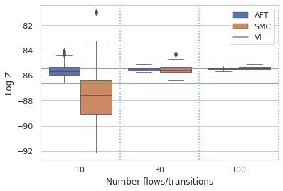
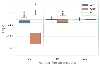
Figure 2: Results from the four different examples. Cyan lines denote gold standard values of the log normalizing constant. In (c) and (d) green horizontal lines denote the median value for an importance sampling estimate based on variational inference. Note that in (d) the small AFT error bars can make it difficult to see - it can be found next to the gold standard value in each case.

6.2 Funnel distribution

We next evaluate the performance of the method on Neal’s ten-dimensional ‘funnel’ distribution (Neal, 2003):

x0\displaystyle x_{0} ∼𝒩(0,σf2),x1:9|x0\displaystyle\sim\mathcal{N}(0,\sigma_{f}^{2}),\quad x_{1:9}|x_{0} ∼𝒩⁡(𝟎,exp⁡(x0)​𝐈).\displaystyle\sim\mathcal{N}(\mathbf{0},\exp(x_{0})\mathbf{I}). (33)

Here, σf2=9\sigma_{f}^{2}=9. Many MCMC methods find this example challenging because there is a variety of length scales depending on the value of x0x_{0} and because marginally x1:9x_{1:9} has heavy tails. We use here slice sampling instead of HMC for the Markov kernels as recommended in (Neal, 2003). For each flow we use an affine inverse autoregressive flow (Kingma et al., 2016). In this example, we also compare against VI (Rezende et al., 2014) which uses the same number of flows. We then apply a simple importance correction to the VI samples to give an unbiased estimate of the normalizing constant. Figure 2 (b) shows the results. We see that for small number of flows/transitions VI performs best, followed by AFT. However, VI shows little further improvement with additional flows and in this regime AFT, SMC and VI perform similarly.

6.3 Variational Autoencoder latent space

For our next example, we trained a variational autoencoder (Kingma and Welling, 2014; Rezende et al., 2014) with convolution on the binarized MNIST dataset (Salakhutdinov and Murray, 2008) and a normal encoder distribution with diagonal covariance. Using the fixed, trained, generative decoder network we investigated the quality of normalizing constant estimation which in this case corresponds to the likelihood of a data point with the distribution over the 30 latent variables marginalized out (Wu et al., 2017).

Using long run SMC on the 10000 point test set we estimate that the hold out log-likelihood per data point for the network is -86.3. For each data point we also found the optimal variational normal approximation with diagonal covariance rather than using the amortized variational approximation. Using this optimal normal approximation we investigated its variance when used as an importance proposal for the likelihood. We estimate the mean absolute error for the estimator across the test set was 0.6 nats per data point which indicates that the VI is often performing well. There was a tail of digits where VI performed relatively worse. Since these ‘difficult’ digits constituted a more challenging inference problem, we used one of these, with a VI/SMC error of 1.5 nats, to comparatively benchmark AFT in the detailed manner used in our other examples.

For the AFT flow we used an affine transformation with diagonal linear transformation matrix. The baseline VI approximation can be thought of the pushforward of a standard normal through this ‘diagonal affine’ flow. Note that since diagonal affine transformations are closed under composition there would obtain no additional expressiveness in the baseline VI approximation from adding more of them.

Figure 2 (c) shows the results for this example. Both AFT and SMC reduce in variance as the number of temperatures increases and exceed the performance of the variational baseline. AFT has a notably lower variance than SMC for 10 and 30 temperatures- which shows the incorporation of the flows is beneficial in this case. Results for other difficult digits are shown in the appendix where the qualitative trend is similar.

6.4 Log Gaussian Cox process

We evaluate here the performance of AFT for estimating the normalizing constant of a log Gaussian Cox process applied to modelling the positions of pine saplings in Finland (Møller et al., 1998). We consider points on a discretized d=M×M=1600d=M\times M=1600 grid. This results in the target density

γ(x)=𝒩(x;μ,K)∏i∈[1:M]2exp(xiyi−aexp(xi)).\gamma(x)=\mathcal{N}(x;\mu,K)\prod_{i\in[1:M]^{2}}\exp(x_{i}y_{i}-a\exp(x_{i})). (34)

This challenging high-dimensional problem is a commonly used benchmark in the SMC literature (Heng et al., 2020; Buchholz et al., 2021). The mean and covariance function match those estimated by (Møller et al., 1998) and are detailed in the Appendix. The supplement also discusses the effect of pre-conditioners on the mixing of the Markov kernel. For the NF we again used the diagonal affine transformation. The approximating family is the push forward of the previous target distribution and thus even a simple flow can result in a good approximation. It is also fast to evaluate. Figure 2 (d) shows that the baseline VI approximation is unable to capture the posterior correlation and that AFT gives significantly more accurate results than SMC for a given number of transitions. As such, the Markov kernel and flow complement each other in this case.

7 Conclusion

We proposed Annealed Flow Transport which combines SMC samplers and normalizing flows. We studied its asymptotic behavior and showed the benefit of introducing learned flows to reduce the asymptotic variance. We identified the scaling limit of AFT as a controlled Feynman–Kac measure whose optimal control solved a flow transport problem in an idealized setting. Empirically we found multiple cases where trained AFT gave lower variance estimates than SMC for the same number of transitions, showing that we can combine the advantages of both SMC and normalizing flows. We believe AFT will be particularly useful in scenarios where it is both difficult to design fast mixing MCMC kernels and very good flows so that neither SMC nor VI provide low variance estimates.

8 Acknowledgements

The authors would like to thank Danilo Rezende, Arthur Gretton and Taylan Cemgil.

References

  • Akyildiz and Míguez, (2020) Akyildiz, Ö. D. and Míguez, J. (2020). Nudging the particle filter. Statistics and Computing, 30(2):305–330.
  • Barash et al., (2017) Barash, L. Y., Weigel, M., Borovskỳ, M., Janke, W., and Shchur, L. N. (2017). GPU accelerated population annealing algorithm. Computer Physics Communications, 220:341–350.
  • Beskos et al., (2016) Beskos, A., Jasra, A., Kantas, N., and Thiery, A. (2016). On the convergence of adaptive sequential Monte Carlo methods. The Annals of Applied Probability, 26(2):1111–1146.
  • Beskos et al., (2011) Beskos, A., Pinski, F., Sanz-Serna, J., and Stuart, A. (2011). Hybrid Monte Carlo on Hilbert spaces. Stochastic Processes and their Applications, 121(10):2201 – 2230.
  • Bradbury et al., (2018) Bradbury, J., Frostig, R., Hawkins, P., Johnson, M. J., Leary, C., Maclaurin, D., Necula, G., Paszke, A., VanderPlas, J., Wanderman-Milne, S., and Zhang, Q. (2018). JAX: composable transformations of Python+NumPy programs.
  • Buchholz et al., (2021) Buchholz, A., Chopin, N., and Jacob, P. E. (2021). Adaptive tuning of Hamiltonian Monte Carlo within sequential Monte Carlo. Bayesian Analysis to appear - arXiv preprint arXiv:1808.07730.
  • Caterini et al., (2018) Caterini, A. L., Doucet, A., and Sejdinovic, D. (2018). Hamiltonian variational auto-encoder. In Advances in Neural Information Processing Systems, pages 8167–8177.
  • Choi, (2019) Choi, M. C. (2019). Universality of the Langevin diffusion as scaling limit of a family of Metropolis–Hastings processes i: fixed dimension. arXiv preprint arXiv:1907.10318.
  • Chopin, (2002) Chopin, N. (2002). A sequential particle filter method for static models. Biometrika, 89(3):539–552.
  • Chopin, (2004) Chopin, N. (2004). Central limit theorem for sequential Monte Carlo methods and its application to Bayesian inference. The Annals of Statistics, 32(6):2385–2411.
  • Crooks, (1998) Crooks, G. E. (1998). Nonequilibrium measurements of free energy differences for microscopically reversible Markovian systems. Journal of Statistical Physics, 90(5-6):1481–1487.
  • Dai et al., (2020) Dai, C., Heng, J., Jacob, P. E., and Whiteley, N. (2020). An invitation to sequential Monte Carlo samplers. arXiv preprint arXiv:2007.11936.
  • Dalalyan, (2017) Dalalyan, A. S. (2017). Theoretical guarantees for approximate sampling from smooth and log-concave densities. Journal of the Royal Statistical Society: Series B, 3(79):651–676.
  • Del Moral, (2004) Del Moral, P. (2004). Feynman-Kac Formulae: Genealogical and Interacting Particle Approximations. Springer.
  • Del Moral et al., (2006) Del Moral, P., Doucet, A., and Jasra, A. (2006). Sequential Monte Carlo samplers. Journal of the Royal Statistical Society: Series B, 68(3):411–436.
  • (16) Del Moral, P., Doucet, A., and Jasra, A. (2012a). An adaptive sequential Monte Carlo method for approximate Bayesian computation. Statistics and Computing, 22(5):1009–1020.
  • (17) Del Moral, P., Doucet, A., and Jasra, A. (2012b). On adaptive resampling strategies for sequential Monte Carlo methods. Bernoulli, 18(1):252–278.
  • Dillon et al., (2017) Dillon, J. V., Langmore, I., Tran, D., Brevdo, E., Vasudevan, S., Moore, D., Patton, B., Alemi, A., Hoffman, M., and Saurous, R. A. (2017). TensorFlow Distributions. arXiv preprint arXiv:1711.10604.
  • Domke and Sheldon, (2018) Domke, J. and Sheldon, D. R. (2018). Importance weighting and variational inference. In Advances in Neural Information Processing Systems, pages 4470–4479.
  • Douc and Moulines, (2008) Douc, R. and Moulines, E. (2008). Limit theorems for weighted samples with applications to sequential Monte Carlo methods. The Annals of Statistics, 36(5):2344–2376.
  • Dudley, (2018) Dudley, R. M. (2018). Real analysis and Probability. CRC Press.
  • Durkan et al., (2019) Durkan, C., Bekasov, A., Murray, I., and Papamakarios, G. (2019). Neural spline flows. In Advances in Neural Information Processing Systems.
  • El Moselhy and Marzouk, (2012) El Moselhy, T. A. and Marzouk, Y. M. (2012). Bayesian inference with optimal maps. Journal of Computational Physics, 231(23):7815–7850.
  • Everitt et al., (2020) Everitt, R. G., Culliford, R., Medina-Aguayo, F., and Wilson, D. J. (2020). Sequential Monte Carlo with transformations. Statistics and Computing, 30(3):663–676.
  • Gao et al., (2020) Gao, C., Isaacson, J., and Krause, C. (2020). i-flow: High-dimensional Integration and Sampling with normalizing flows. arXiv preprint arXiv:2001.05486.
  • Gelfand and Mitter, (1991) Gelfand, S. B. and Mitter, S. K. (1991). Weak convergence of Markov chain sampling methods and annealing algorithms to diffusions. Journal of Optimization Theory and Applications, 68(3):483–498.
  • Germain et al., (2015) Germain, M., Gregor, K., Murray, I., and Larochelle, H. (2015). Made: Masked autoencoder for distribution estimation. In Bach, F. and Blei, D., editors, Proceedings of the 32nd International Conference on Machine Learning, volume 37 of Proceedings of Machine Learning Research, pages 881–889, Lille, France. PMLR.
  • Gilks and Berzuini, (2001) Gilks, W. R. and Berzuini, C. (2001). Following a moving target - Monte Carlo inference for dynamic Bayesian models. Journal of the Royal Statistical Society: Series B, 63(1):127–146.
  • Goyal et al., (2017) Goyal, A. G. A. P., Ke, N. R., Ganguli, S., and Bengio, Y. (2017). Variational walkback: Learning a transition operator as a stochastic recurrent net. In Advances in Neural Information Processing Systems, pages 4392–4402.
  • Guarniero et al., (2017) Guarniero, P., Johansen, A. M., and Lee, A. (2017). The iterated auxiliary particle filter. Journal of the American Statistical Association, 112(520):1636–1647.
  • Han and Liu, (2017) Han, J. and Liu, Q. (2017). Stein variational adaptive importance sampling. Uncertainty in Artificial Intelligence.
  • Heng et al., (2020) Heng, J., Bishop, A. N., Deligiannidis, G., and Doucet, A. (2020). Controlled sequential Monte Carlo. The Annals of Statistics, 48(5):2904–2929.
  • Heng et al., (2021) Heng, J., Doucet, A., and Pokern, Y. (2021). Gibbs flow for approximate transport with applications to Bayesian computation. Journal of the Royal Statistical Society Series B, 83(1):156–187.
  • Hennigan et al., (2020) Hennigan, T., Cai, T., Norman, T., and Babuschkin, I. (2020). Haiku: Sonnet for JAX.
  • Hessel et al., (2020) Hessel, M., Budden, D., Viola, F., Rosca, M., Sezener, E., and Hennigan, T. (2020). Optax: composable gradient transformation and optimisation, in jax.
  • Hoffman, (2017) Hoffman, M. D. (2017). Learning deep latent Gaussian models with Markov chain Monte Carlo. In Precup, D. and Teh, Y. W., editors, Proceedings of the 34th International Conference on Machine Learning, volume 70 of Proceedings of Machine Learning Research, pages 1510–1519. PMLR.
  • Huang et al., (2018) Huang, C.-W., Tan, S., Lacoste, A., and Courville, A. C. (2018). Improving explorability in variational inference with annealed variational objectives. In Advances in Neural Information Processing Systems, pages 9701–9711.
  • Huang et al., (2020) Huang, S., Makhzani, A., Cao, Y., and Grosse, R. (2020). Evaluating lossy compression rates of deep generative models. In International Conference on Machine Learning, pages 4444–4454. PMLR.
  • Hukushima and Iba, (2003) Hukushima, K. and Iba, Y. (2003). Population annealing and its application to a spin glass. In AIP Conference Proceedings, volume 690, pages 200–206. American Institute of Physics.
  • Jarzynski, (1997) Jarzynski, C. (1997). Nonequilibrium equality for free energy differences. Physical Review Letters, 78(14):2690–2963.
  • Jasra et al., (2011) Jasra, A., Stephens, D. A., Doucet, A., and Tsagaris, T. (2011). Inference for Lévy-driven stochastic volatility models via adaptive sequential Monte Carlo. Scandinavian Journal of Statistics, 38(1):1–22.
  • Kappen and Ruiz, (2016) Kappen, H. J. and Ruiz, H. C. (2016). Adaptive importance sampling for control and inference. Journal of Statistical Physics, 162(5):1244–1266.
  • Kingma and Ba, (2014) Kingma, D. P. and Ba, J. (2014). Adam: A method for stochastic optimization. arXiv preprint arXiv:1412.6980.
  • Kingma et al., (2016) Kingma, D. P., Salimans, T., Jozefowicz, R., Chen, X., Sutskever, I., and Welling, M. (2016). Improved variational inference with inverse autoregressive flow. In Lee, D., Sugiyama, M., Luxburg, U., Guyon, I., and Garnett, R., editors, Advances in Neural Information Processing Systems, volume 29. Curran Associates, Inc.
  • Kingma and Welling, (2014) Kingma, D. P. and Welling, M. (2014). Auto-encoding variational Bayes. ICLR.
  • Kitagawa, (1996) Kitagawa, G. (1996). Monte Carlo filter and smoother for non-Gaussian nonlinear state space models. Journal of Computational and Graphical Statistics, 5(1):1–25.
  • Künsch, (2005) Künsch, H. R. (2005). Recursive Monte Carlo filters: algorithms and theoretical analysis. The Annals of Statistics, 33(5):1983–2021.
  • Le et al., (2018) Le, T. A., Igl, M., Rainforth, T., Jin, T., and Wood, F. (2018). Auto-encoding sequential Monte Carlo. In ICLR.
  • Lee et al., (2010) Lee, A., Yau, C., Giles, M. B., Doucet, A., and Holmes, C. C. (2010). On the utility of graphics cards to perform massively parallel simulation of advanced monte carlo methods. Journal of Computational and Graphical Statistics, 19(4):769–789.
  • Lei Ba et al., (2016) Lei Ba, J., Kiros, J. R., and Hinton, G. E. (2016). Layer Normalization. arXiv e-prints.
  • Lelièvre et al., (2010) Lelièvre, T., Rousset, M., and Stoltz, G. (2010). Free Energy Computations: A Mathematical Perspective. World Scientific.
  • Li and Chen, (2019) Li, Q. and Chen, Y. (2019). Rate distortion via deep learning. IEEE Transactions on Communications, 68(1):456–465.
  • Liu et al., (2019) Liu, C., Zhuo, J., Cheng, P., Zhang, R., and Zhu, J. (2019). Understanding and accelerating particle-based variational inference. In International Conference on Machine Learning, pages 4082–4092.
  • Liu and Chen, (1995) Liu, J. S. and Chen, R. (1995). Blind deconvolution via sequential imputations. Journal of the American Statistical Association, 90(430):567–576.
  • Liu and Wang, (2016) Liu, Q. and Wang, D. (2016). Stein variational gradient descent: a general purpose Bayesian inference algorithm. In Advances in Neural Information Processing Systems.
  • Llorente et al., (2020) Llorente, F., Martino, L., Delgado, D., and Lopez-Santiago, J. (2020). Marginal likelihood computation for model selection and hypothesis testing: an extensive review. arXiv preprint arXiv:2005.08334.
  • MacEachern et al., (1999) MacEachern, S. N., Clyde, M., and Liu, J. S. (1999). Sequential importance sampling for nonparametric Bayes models: The next generation. Canadian Journal of Statistics, 27(2):251–267.
  • Maddison et al., (2017) Maddison, C. J., Lawson, J., Tucker, G., Heess, N., Norouzi, M., Mnih, A., Doucet, A., and Teh, Y. (2017). Filtering variational objectives. In Advances in Neural Information Processing Systems, pages 6573–6583.
  • Marzouk et al., (2016) Marzouk, Y., Moselhy, T., Parno, M., and Spantini, A. (2016). Sampling via measure transport: An introduction. Handbook of Uncertainty Quantification, pages 1–41.
  • Mnih and Rezende, (2016) Mnih, A. and Rezende, D. (2016). Variational inference for Monte Carlo objectives. In International Conference on Machine Learning, pages 2188–2196. PMLR.
  • Møller et al., (1998) Møller, J., Syversveen, A. R., and Waagepetersen, R. P. (1998). Log Gaussian Cox processes. Scandinavian Journal of Statistics, 25(3):451–482.
  • Naesseth et al., (2018) Naesseth, C. A., Linderman, S. W., Ranganath, R., and Blei, D. M. (2018). Variational sequential Monte Carlo. In AISTATS.
  • Neal, (2011) Neal, R. (2011). MCMC using Hamiltonian dynamics. Handbook of Markov chain Monte Carlo.
  • Neal, (2001) Neal, R. M. (2001). Annealed importance sampling. Statistics and Computing, 11(2):125–139.
  • Neal, (2003) Neal, R. M. (2003). Slice sampling. The Annals of Statistics, 31(3):705–767.
  • Nicoli et al., (2020) Nicoli, K. A., Nakajima, S., Strodthoff, N., Samek, W., Müller, K.-R., and Kessel, P. (2020). Asymptotically unbiased estimation of physical observables with neural samplers. Physical Review E, 101(2):023304.
  • Noé et al., (2019) Noé, F., Olsson, S., Köhler, J., and Wu, H. (2019). Boltzmann generators: Sampling equilibrium states of many-body systems with deep learning. Science, 365(6457):eaaw1147.
  • Olmez et al., (2020) Olmez, S. Y., Taghvaei, A., and Mehta, P. G. (2020). Deep fpf: Gain function approximation in high-dimensional setting. In 59th IEEE Conference on Decision and Control (CDC), pages 4790–4795. IEEE.
  • Papamakarios et al., (2019) Papamakarios, G., Nalisnick, E., Rezende, D. J., Mohamed, S., and Lakshminarayanan, B. (2019). Normalizing flows for probabilistic modeling and inference. arXiv preprint arXiv:1912.02762.
  • Reich, (2011) Reich, S. (2011). A dynamical systems framework for intermittent data assimilation. BIT Numerical Mathematics, 51(1):235–249.
  • Reich and Weissmann, (2021) Reich, S. and Weissmann, S. (2021). Fokker–Planck particle systems for Bayesian inference: Computational approaches. SIAM/ASA Journal on Uncertainty Quantification, 9(2):446–482.
  • Rezende and Mohamed, (2015) Rezende, D. J. and Mohamed, S. (2015). Variational inference with normalizing flows. In Proceedings of the 32nd International Conference on Machine Learning - Volume 37, ICML’15, pages 1530–1538. JMLR.org.
  • Rezende et al., (2014) Rezende, D. J., Mohamed, S., and Wierstra, D. (2014). Stochastic backpropagation and approximate inference in deep generative models. In ICML, pages 1278–1286.
  • Richard and Zhang, (2007) Richard, J.-F. and Zhang, W. (2007). Efficient high-dimensional importance sampling. Journal of Econometrics, 141(2):1385–1411.
  • Rousset and Stoltz, (2006) Rousset, M. and Stoltz, G. (2006). Equilibrium sampling from nonequilibrium dynamics. Journal of Statistical Physics, 123(6):1251–1272.
  • Salakhutdinov and Murray, (2008) Salakhutdinov, R. and Murray, I. (2008). On the quantitative analysis of Deep Belief Networks. In Proceedings of the 25th Annual International Conference on Machine Learning (ICML 2008), pages 872–879.
  • Salimans et al., (2015) Salimans, T., Kingma, D., and Welling, M. (2015). Markov chain Monte Carlo and variational inference: Bridging the gap. In International Conference on Machine Learning, pages 1218–1226.
  • Schäfer and Chopin, (2013) Schäfer, C. and Chopin, N. (2013). Sequential Monte Carlo on large binary sampling spaces. Statistics and Computing, 23(2):163–184.
  • Sen, (2018) Sen, B. (2018). A gentle introduction to empirical process theory and applications. Lecture Notes, Columbia University.
  • Taghvaei et al., (2020) Taghvaei, A., Mehta, P. G., and Meyn, S. P. (2020). Diffusion map-based algorithm for gain function approximation in the feedback particle filter. SIAM/ASA Journal on Uncertainty Quantification, 8(3):1090–1117.
  • Thin et al., (2021) Thin, A., Kotelevskii, N., Durmus, A., Panov, M., Moulines, E., and Doucet, A. (2021). Monte Carlo variational auto-encoders. International Conference on Machine Learning.
  • Turner and Sahani, (2011) Turner, R. E. and Sahani, M. (2011). Two problems with variational expectation maximisation for time-series models. In Barber, D., Cemgil, T., and Chiappa, S., editors, Bayesian Time Series Models, chapter 5, pages 109–130. Cambridge University Press.
  • Vaikuntanathan and Jarzynski, (2008) Vaikuntanathan, S. and Jarzynski, C. (2008). Escorted free energy simulations: Improving convergence by reducing dissipation. Physical Review Letters, 100(19):190601.
  • Vaikuntanathan and Jarzynski, (2011) Vaikuntanathan, S. and Jarzynski, C. (2011). Escorted free energy simulations. The Journal of Chemical Physics, 134(5):054107.
  • Van der Vaart, (2000) Van der Vaart, A. W. (2000). Asymptotic Statistics. Cambridge University Press.
  • Wang and Li, (2019) Wang, Y. and Li, W. (2019). Accelerated information gradient flow. arXiv preprint arXiv:1909.02102.
  • Wirnsberger et al., (2020) Wirnsberger, P., Ballard, A. J., Papamakarios, G., Abercrombie, S., Racanière, S., Pritzel, A., Rezende, D., and Blundell, C. (2020). Targeted free energy estimation via learned mappings. The Journal of Chemical Physics, 153(14):144112.
  • Wu et al., (2020) Wu, H., Köhler, J., and Noé, F. (2020). Stochastic normalizing flows. In Advances in Neural Information Processing Systems.
  • Wu et al., (2017) Wu, Y., Burda, Y., Salakhutdinov, R., and Grosse, R. B. (2017). On the quantitative analysis of decoder-based generative models. In 5th International Conference on Learning Representations, ICLR 2017, Toulon, France, April 24-26, 2017, Conference Track Proceedings.
  • Zhou et al., (2016) Zhou, Y., Johansen, A. M., and Aston, J. A. (2016). Toward automatic model comparison: An adaptive sequential Monte Carlo approach. Journal of Computational and Graphical Statistics, 25(3):701–726.
  • Zhu et al., (2020) Zhu, M., Liu, C., and Zhu, J. (2020). Variance reduction and quasi-Newton for particle-based variational inference. In International Conference on Machine Learning, pages 11576–11587.

Appendix A Using measure-theoretic notation

The Markov transition kernel MkM_{k} is defined as a map Mk:𝒳×ℬ⁡(𝒳)→[0,1]M_{k}:\mathcal{X}\times\mathcal{B}(\mathcal{X})\rightarrow[0,1] where ℬ⁡(𝒳)\mathcal{B}(\mathcal{X}) are the Borel sets, Lk−1L_{k-1} is defined similarly. The joint distribution of the non-homogeneous Markov chain of initial distribution X0∼π0X_{0}\sim\pi_{0} and Markov transition kernel Xl∼Ml​(Xl−1,⋅)X_{l}\sim M_{l}(X_{l-1},\cdot) at time ll is given at time kk by

η¯k(dx0:k)=π0(dx0)∏l=1kMl(xl−1,dxl).\displaystyle\bar{\eta}_{k}(\mathop{}\!\mathrm{d}x_{0:k})=\pi_{0}(\mathop{}\!\mathrm{d}x_{0})\prod_{l=1}^{k}M_{l}(x_{l-1},\mathop{}\!\mathrm{d}x_{l}). (35)

SMC samplers rely on the following target distribution of the form

π¯k(dx0:k)=πk(dxk)∏l=0k−1Ll(xl+1,dxl),\displaystyle\bar{\pi}_{k}(\mathop{}\!\mathrm{d}x_{0:k})=\pi_{k}(\mathop{}\!\mathrm{d}x_{k})\prod_{l=0}^{k-1}L_{l}(x_{l+1},\mathop{}\!\mathrm{d}x_{l}), (36)

and γk(dx0:k)=Zkπ¯k(dx0:k)\gamma_{k}(\mathop{}\!\mathrm{d}x_{0:k})=Z_{k}\bar{\pi}_{k}(\mathop{}\!\mathrm{d}x_{0:k}). When πl​(⁡d​x′)​Ll−1​(x′,⁡d​x)\pi_{l}(\mathop{}\!\mathrm{d}x^{\prime})L_{l-1}(x^{\prime},\mathop{}\!\mathrm{d}x) is absolutely continuous w.r.t. πl​(⁡d​x)​Ml​(x,⁡d​x′)\pi_{l}(\mathop{}\!\mathrm{d}x)M_{l}(x,\mathop{}\!\mathrm{d}x^{\prime}), then we can define its Radon-Nikodym derivative and the incremental importance weight GlG_{l} through

Gl​(xl−1,xl)=ZlZl−1​πl​(⁡d​xl)​Ll−1​(xl,⁡d​xl−1)πl−1​(⁡d​xl−1)​Ml​(xl−1,⁡d​xl)=γl​(⁡d​xl)​Ll−1​(xl,⁡d​xl−1)γl−1​(⁡d​xl−1)​Ml​(xl−1,⁡d​xl).\displaystyle G_{l}(x_{l-1},x_{l})=\frac{Z_{l}}{Z_{l-1}}\frac{\pi_{l}(\mathop{}\!\mathrm{d}x_{l})L_{l-1}(x_{l},\mathop{}\!\mathrm{d}x_{l-1})}{\pi_{l-1}(\mathop{}\!\mathrm{d}x_{l-1})M_{l}(x_{l-1},\mathop{}\!\mathrm{d}x_{l})}=\frac{\gamma_{l}(\mathop{}\!\mathrm{d}x_{l})L_{l-1}(x_{l},\mathop{}\!\mathrm{d}x_{l-1})}{\gamma_{l-1}(\mathop{}\!\mathrm{d}x_{l-1})M_{l}(x_{l-1},\mathop{}\!\mathrm{d}x_{l})}. (37)

If GlG_{l} is defined for l=1,…,kl=1,...,k, then π¯k\bar{\pi}_{k} is absolutely continuous w.r.t. η¯k\bar{\eta}_{k} so we can write

π¯k[f]=η¯k​[wk​f]η¯k​[wk],wherewk(x0:k)=Zk⁡d​π¯k⁡d​η¯k(x0:k)=⁡d​γ¯k⁡d​η¯k(x0:k)=∏l=1kGl(xl−1,xl).\displaystyle\quad\bar{\pi}_{k}[f]=\frac{\bar{\eta}_{k}[w_{k}f]}{\bar{\eta}_{k}[w_{k}]},\quad\text{where}\quad w_{k}(x_{0:k})=Z_{k}\frac{\mathop{}\!\mathrm{d}\bar{\pi}_{k}}{\mathop{}\!\mathrm{d}\bar{\eta}_{k}}(x_{0:k})=\frac{\mathop{}\!\mathrm{d}\bar{\gamma}_{k}}{\mathop{}\!\mathrm{d}\bar{\eta}_{k}}(x_{0:k})=\prod_{l=1}^{k}G_{l}(x_{l-1},x_{l}). (38)

If MkM_{k} is πk\pi_{k}-invariant then (Crooks, 1998; Neal, 2001) select Lk−1L_{k-1} at the reversal of MkM_{k}, that is the kernel satisfying πk​(⁡d​x)​Mk​(x,⁡d​x′)=πk​(⁡d​x′)​Lk−1​(x′,⁡d​x)\pi_{k}(\mathop{}\!\mathrm{d}x)M_{k}(x,\mathop{}\!\mathrm{d}x^{\prime})=\pi_{k}(\mathop{}\!\mathrm{d}x^{\prime})L_{k-1}(x^{\prime},\mathop{}\!\mathrm{d}x) and in this case

Gl​(xl−1,xl)=ZlZl−1​⁡d​πl⁡d​πl−1​(xl−1)=⁡d​γl⁡d​γl−1​(xl−1).G_{l}(x_{l-1},x_{l})=\frac{Z_{l}}{Z_{l-1}}\frac{\mathop{}\!\mathrm{d}\pi_{l}}{\mathop{}\!\mathrm{d}\pi_{l-1}}(x_{l-1})=\frac{\mathop{}\!\mathrm{d}\gamma_{l}}{\mathop{}\!\mathrm{d}\gamma_{l-1}}(x_{l-1}). (39)

Appendix B Extended proposal and target of AFT algorithm

In this section, assuming the transport maps TkT_{k} are here fixed, we write explicitly the extended proposal and target distributions used implicitly by the AFT algorithm if no resampling was used.

B.1 Non-collapsed version

In this case, we sample X0∼π0​(⋅)X_{0}\sim\pi_{0}(\cdot) at k=0k=0 then use X~k=Tk​(Xk−1)\tilde{X}_{k}=T_{k}(X_{k-1}) followed by Xk=Kk​(X~k,⋅)X_{k}=K_{k}(\tilde{X}_{k},\cdot) at time k≥1k\geq 1. Hence, using the notation Mltrans​(x,x′)=δTl​(x)​(x′)M^{\textup{trans}}_{l}(x,x^{\prime})=\delta_{T_{l}(x)}(x^{\prime}) and Mlmut​(x,x′)=Kl​(x,x′)M^{\textup{mut}}_{l}(x,x^{\prime})=K_{l}(x,x^{\prime}), the proposal at time kk after the transport step is of the form

η¯k(x0:k−1,x~1:k)=π0(x0)(∏l=1k−1Mltrans(xl−1,x~l)Mlmut(x~l,xl))Mktrans(xk−1,x~k),\bar{\eta}_{k}(x_{0:k-1},\tilde{x}_{1:k})=\pi_{0}(x_{0})\left(\prod_{l=1}^{k-1}M^{\textup{trans}}_{l}(x_{l-1},\tilde{x}_{l})M^{\textup{mut}}_{l}(\tilde{x}_{l},x_{l})\right)M^{\textup{trans}}_{k}(x_{k-1},\tilde{x}_{k}), (40)

and the target is

π¯k(x0:k−1,x~1:k)=πk(x~k)Lk−1trans(x~k,xk−1)(∏l=0k−2Llmut(xl+1,x~l+1)Lltrans(x~l+1,xl)),\bar{\pi}_{k}(x_{0:k-1},\tilde{x}_{1:k})=\pi_{k}(\tilde{x}_{k})L^{\textup{trans}}_{k-1}(\tilde{x}_{k},x_{k-1})\left(\prod_{l=0}^{k-2}L^{\textup{mut}}_{l}(x_{l+1},\tilde{x}_{l+1})L^{\textup{trans}}_{l}(\tilde{x}_{l+1},x_{l})\right), (41)

where Ll−1trans​(x,x′)=δTl−1​(x)​(x′)L^{\textup{trans}}_{l-1}(x,x^{\prime})=\delta_{T^{-1}_{l}(x)}(x^{\prime}) and Ll−1mul​(x,x′)=πl​(x′)​Mlmul​(x′,x)/πl​(x)L^{\textup{mul}}_{l-1}(x,x^{\prime})=\pi_{l}(x^{\prime})M^{\textup{mul}}_{l}(x^{\prime},x)/\pi_{l}(x). After the mutation step at time kk, the proposal is

η¯k(x0:k,x~1:k)=η¯k(x0:k−1,x~1:k)Mkmut(x~k,xk)=π0(x0)(∏l=1kMltrans(xl−1,x~l)Mlmut(x~l,xl)).\bar{\eta}_{k}(x_{0:k},\tilde{x}_{1:k})=\bar{\eta}_{k}(x_{0:k-1},\tilde{x}_{1:k})M^{\textup{mut}}_{k}(\tilde{x}_{k},x_{k})=\pi_{0}(x_{0})\left(\prod_{l=1}^{k}M^{\textup{trans}}_{l}(x_{l-1},\tilde{x}_{l})M^{\textup{mut}}_{l}(\tilde{x}_{l},x_{l})\right). (42)

and the target is

π¯k(x0:k,x~1:k)=πk(xk)(∏l=0k−1Llmut(xl+1,x~l+1)Lltrans(x~l+1,xl)).\bar{\pi}_{k}(x_{0:k},\tilde{x}_{1:k})=\pi_{k}(x_{k})\left(\prod_{l=0}^{k-1}L^{\textup{mut}}_{l}(x_{l+1},\tilde{x}_{l+1})L^{\textup{trans}}_{l}(\tilde{x}_{l+1},x_{l})\right). (43)

Hence the incremental weight after a transport term at time kk is of the form

π¯k(x0:k−1,x~1:k)η¯k(x0:k−1,x~1:k)=π¯k−1(x0:k−1,x~1:k−1)η¯k−1(x0:k−1,x~1:k−1)πk​(x~k)​Lk−1trans​(x~k,xk−1)πk−1​(x~k−1)​Mktrans​(xk−1,x~k)⏟incremental weight=Zk−1Zk​Gk,Tk​(xk−1),\frac{\bar{\pi}_{k}(x_{0:k-1},\tilde{x}_{1:k})}{\bar{\eta}_{k}(x_{0:k-1},\tilde{x}_{1:k})}=\frac{\bar{\pi}_{k-1}(x_{0:k-1},\tilde{x}_{1:k-1})}{\bar{\eta}_{k-1}(x_{0:k-1},\tilde{x}_{1:k-1})}\underbrace{\frac{\pi_{k}(\tilde{x}_{k})L^{\textup{trans}}_{k-1}(\tilde{x}_{k},x_{k-1})}{\pi_{k-1}(\tilde{x}_{k-1})M^{\textup{trans}}_{k}(x_{k-1},\tilde{x}_{k})}}_{\textup{incremental weight}=\frac{Z_{k-1}}{Z_{k}}G_{k,T_{k}}(x_{k-1})}, (44)

while after the mutation step it is of the form

π¯k(x0:k,x~1:k)η¯k(x0:k,x~1:k)=π¯k(x0:k−1,x~1:k)η¯k(x0:k−1,x~1:k)πk​(xk)​Lk−1mul​(xk,x~k)πk​(x~k)​Mkmul​(x~k,xk)⏟incremental weight=1.\frac{\bar{\pi}_{k}(x_{0:k},\tilde{x}_{1:k})}{\bar{\eta}_{k}(x_{0:k},\tilde{x}_{1:k})}=\frac{\bar{\pi}_{k}(x_{0:k-1},\tilde{x}_{1:k})}{\bar{\eta}_{k}(x_{0:k-1},\tilde{x}_{1:k})}\underbrace{\frac{\pi_{k}(x_{k})L^{\textup{mul}}_{k-1}(x_{k},\tilde{x}_{k})}{\pi_{k}(\tilde{x}_{k})M^{\textup{mul}}_{k}(\tilde{x}_{k},x_{k})}}_{\textup{incremental weight}=1}. (45)

B.2 Collapsed version

When no resampling is used, there is no use for the introduction of the random variables X~1:k\tilde{X}_{1:k} in the previous derivation and they can be integrated out. In this case, we collapse the transport step and mutation step into one single Markov kernel

Mkcol​(x,x′)\displaystyle M_{k}^{\textup{col}}(x,x^{\prime}) =∫Mktrans​(x,x~)​Mkmut​(x~,x′)​⁡𝑑x~\displaystyle=\int M^{\textup{trans}}_{k}(x,\tilde{x})M^{\textup{mut}}_{k}(\tilde{x},x^{\prime})\mathop{}\!\mathrm{d}\tilde{x} (46)
=∫δTk​(x)​(x~)​Kk​(x~,x′)​⁡𝑑x~\displaystyle=\int\delta_{T_{k}(x)}(\tilde{x})K_{k}(\tilde{x},x^{\prime})\mathop{}\!\mathrm{d}\tilde{x} (47)
=Kk​(Tk​(x),x′).\displaystyle=K_{k}(T_{k}(x),x^{\prime}). (48)

Similarly we collapse the backward kernels used to defined the extended target distributions π¯k\bar{\pi}_{k}

Lk−1col​(x,x′)\displaystyle L_{k-1}^{\textup{col}}(x,x^{\prime}) =∫πk​(x~)​Kk​(x~,x)πk​Kk​(x)​δTk−1​(x~)​(x′)​⁡𝑑x~\displaystyle=\int\frac{\pi_{k}(\tilde{x})K_{k}(\tilde{x},x)}{\pi_{k}K_{k}(x)}\delta_{T^{-1}_{k}(\tilde{x})}(x^{\prime})\mathop{}\!\mathrm{d}\tilde{x} (49)
=πk​(Tk​(x′))​|∇Tk​(x′)|​Kk​(Tk​(x′),x)πk​Kk​(x).\displaystyle=\frac{\pi_{k}(T_{k}(x^{\prime}))|\nabla T_{k}(x^{\prime})|K_{k}(T_{k}(x^{\prime}),x)}{\pi_{k}K_{k}(x)}. (50)

Contrary to Section B.1, we consider the more general scenario here where KkK_{k} might not be πk\pi_{k} invariant discussed in Section 5. From Equation 46 and Equation 49, π¯k\bar{\pi}_{k} is thus given by (7) for

wk(x0:k)\displaystyle w_{k}(x_{0:k}) =∏l=1kγl​(xl)γl​Kl​(xl)⏟rk(x1:k)∏l=1kGl,Tl(xl−1),\displaystyle=\underbrace{\prod_{l=1}^{k}\frac{\gamma_{l}(x_{l})}{\gamma_{l}K_{l}(x_{l})}}_{\text{$r_{k}(x_{1:k})$}}\prod_{l=1}^{k}G_{l,T_{l}}(x_{l-1}), (52)

where rk(x1:k)=1r_{k}(x_{1:k})=1 for πl\pi_{l}-invariant MCMC kernels KlK_{l} as used in Algorithm 1.

Appendix C Proof of the asymptotic results

We consider the unnormalized empirical measure γkN\gamma_{k}^{N} defined as:

γkN=ZkN​πkN.\displaystyle\gamma_{k}^{N}=Z_{k}^{N}\pi_{k}^{N}. (54)

We will provide the consistency and CLT results for both γkN​[f]\gamma_{k}^{N}[f] and πkN​[f]\pi_{k}^{N}[f] which imply the results on the normalizing constant ZkNZ_{k}^{N} as ZkN=γkN​[1]Z_{k}^{N}=\gamma_{k}^{N}[1]. We denote by ℱkN\mathcal{F}_{k}^{N} the filtration generated by the particles XkiX^{i}_{k} and the NFs Tk+1T_{k+1} up to time kk and write 𝔼k​[f]=𝔼⁡[f|ℱkN]\mathbb{E}_{k}[f]=\mathbb{E}[f|\mathcal{F}_{k}^{N}]. This accounts for possible randomness coming from the optimization of the NFs. We also consider 𝒞p\mathcal{C}_{p} the class of continuous functions ff on 𝒳\mathcal{X} with growth in xx of at most pp, for some non-negative integer pp, i.e.

𝒞p(C)={f:𝒳→ℝ|f is continuous and ∀x∈𝒳:‖f(x)‖≤C(1+‖x‖p)}.\displaystyle\mathcal{C}_{p}(C)=\{f:\mathcal{X}\rightarrow\mathbb{R}\penalty\ |\penalty\ f\text{ is continuous and }\forall x\in\mathcal{X}:{\left\lVert f(x)\right\rVert}\leq C{\left(1+{\left\lVert x\right\rVert}^{p}\right)}\}. (55)

In addition, we denote by ℒ​𝒞p\mathcal{L}\mathcal{C}_{p} the class of functions in 𝒞p\mathcal{C}_{p} that are locally Lipschitz and with local Lipschitz constant satisfying a growth condition:

ℒ𝒞p(C)={f∈𝒞p(C)|∀x,x′∈𝒳:‖f(x)−f(x′)‖≤C(1+‖x‖p+1+‖x′‖p+1)‖x−x′‖}.\displaystyle\mathcal{LC}_{p}(C)={\left\{f\in\mathcal{C}_{p}(C)\penalty\ |\penalty\ \forall x,x^{\prime}\in\mathcal{X}:{\left\lVert f(x)-f(x^{\prime})\right\rVert}\leq C{\left(1+{\left\lVert x\right\rVert}^{p+1}+{\left\lVert x^{\prime}\right\rVert}^{p+1}\right)}{\left\lVert x-x^{\prime}\right\rVert}\right\}}. (56)

For ease of notation we also introduce the unnormalized transition kernel Qk,TQ_{k,T} which acts on functions ff by:

Qk,T​[f]​(x):=Gk,T​(x)​∫f⁡(y)​Kk​(T⁡(x),⁡𝑑y).\displaystyle Q_{k,T}[f](x):=G_{k,T}(x)\int f(y)K_{k}(T(x),\mathop{}\!\mathrm{d}y). (57)

Moreover, we overload the notation and write ℒk​(θ):=ℒk​(τθ)\mathcal{L}_{k}(\theta):=\mathcal{L}_{k}(\tau_{\theta}) and ℒkN​(θ):=ℒkN​(τθ)\mathcal{L}^{N}_{k}(\theta):=\mathcal{L}^{N}_{k}(\tau_{\theta}).

C.1 Assumptions

The following assumptions are needed for both 1 and 2.

  1. (A)

    The Markov kernel KkK_{k} preserves the class 𝒞p\mathcal{C}_{p} for any pp, meaning that Kk​(f)∈𝒞pK_{k}(f)\in\mathcal{C}_{p} whenever ff in 𝒞p\mathcal{C}_{p}.

  2. (B)

    πk\pi_{k} admits 88th order moments.

  3. (C)

    The normalizing flows in 𝒯\mathcal{T} are of the form T​(x)=τθ​(x)T(x)=\tau_{\theta}(x) where θ\theta is a finite dimensional vector in a compact convex set Θ\Theta. Moreover, the maps x↦τθ​(x)x\mapsto\tau_{\theta}(x) are LL-Lipschitz and jointly continuous in xx and θ\theta.

  4. (D)

    The importance weights Gk,T​(x)G_{k,T}(x) are uniformly bounded over xx and TT.

In addition to the previous assumptions, we will need additional assumptions for the CLT result in 2. First, we strengthen (A)

  1. (E)

    The Markov kernel KkK_{k} preserves the class ℒ​𝒞p\mathcal{LC}_{p} for any pp, i.e. Kk​(f)∈𝒞pK_{k}(f)\in\mathcal{C}_{p} for any ff in ℒ​𝒞p\mathcal{LC}_{p}.

We then make additional assumptions on the smoothness of the potentials VkV_{k} and the parameterization of the normalizing flows τθ\tau_{\theta}:

  1. (F)

    The flow (θ,x)↦τθ​(x)(\theta,x)\mapsto\tau_{\theta}(x) admits derivatives ∇θτθ​(x)\nabla_{\theta}\tau_{\theta}(x), ∂θi∂xlτθ​(x)\partial_{\theta_{i}}\partial_{x_{l}}\tau_{\theta}(x) and ∂θi∂θj∂xlτθ​(x)\partial_{\theta_{i}}\partial_{\theta_{j}}\partial_{x_{l}}\tau_{\theta}(x), Hx​τθ​(x)H_{x}\tau_{\theta}(x) with at most linear growth in xx uniformly in θ\theta. Moreover, all singular values of ∇xτθ​(x)\nabla_{x}\tau_{\theta}(x) are lower-bounded by a positive constant c>0c>0 uniformly in xx and θ\theta.

  2. (G)

    The potentials are twice continuously differentiable and their gradients are LL-Lipchitz, i.e. ‖∇Vk​(x)−∇Vk​(x′)‖≤L​‖x−x′‖\|\nabla V_{k}(x)-\nabla V_{k}(x^{\prime})\|\leq L\|x-x^{\prime}\|.

Finally, we make two assumptions on the algorithm used to find θkN\theta^{N}_{k}. We denote by Θk⋆\Theta^{\star}_{k} the set of local minimizers of the population loss θ↦ℒk​(θ)\theta\mapsto\mathcal{L}_{k}(\theta).

  1. (H)

    The estimator θkN\theta_{k}^{N} satisfies:

    ∇ℒkN​(θkN)\displaystyle\nabla\mathcal{L}^{N}_{k}(\theta^{N}_{k}) =oℙ​(1),\displaystyle=o_{\mathbb{P}}(1), (58)
    H​ℒkN​(θkN)\displaystyle H\mathcal{L}^{N}_{k}(\theta^{N}_{k}) ≥oℙ​(1).\displaystyle\geq o_{\mathbb{P}}(1). (59)
  2. (I)

    There exists a local minimizer θk⋆∈Θk⋆\theta^{\star}_{k}\in\Theta^{\star}_{k} of the population loss ℒk​(θ)\mathcal{L}_{k}(\theta) such that

    ℙ[θk⋆∈argminθ∈Θk⋆‖θkN−θ‖]→1.\displaystyle\mathbb{P}{\left[\theta^{\star}_{k}\in\arg\min_{\theta\in\Theta^{\star}_{k}}{\left\lVert\theta^{N}_{k}-\theta\right\rVert}\right]}\rightarrow 1. (61)

(H) states that the algorithm finds an approximate local minimizer of the empirical loss ℒkN​(θ)\mathcal{L}^{N}_{k}(\theta). This condition depends only on how well the algorithm is able to find a local optimum of the empirical loss accurately. In the ideal case where θkN\theta^{N}_{k} is an exact local minimizer of ℒkN​(θ)\mathcal{L}^{N}_{k}(\theta), then the condition holds by definition. (I) states that as NN increases θkN\theta_{k}^{N} remains within the basin of attraction of a single local optimum θk⋆\theta^{\star}_{k} and does not jump between different solutions. For instance, in the case of gradient descent, this assumption can be satisfied if the algorithm starts from the same initial (θk)0(\theta_{k})_{0} for all values of NN and is iterated to obtain an estimator θkN\theta_{k}^{N}. Hence, as NN increases the empirical loss will have the same basins of attraction as the population loss and the choice of the solution θk⋆\theta_{k}^{\star} is determined only by the initial condition (θk)0(\theta_{k})_{0}.

C.2 Kernels satisfying (A) and (E)

Here we provide examples of generic transition kernels KkK_{k} that satisfy (A) and (E). In Section C.2.1, we show that the kernel used in the Unadjusted Langevin Algorithm (ULA kernel) satisfies (A) and (E) under mild assumptions on πk\pi_{k}. While this kernel is not exactly invariant w.r.t. πk\pi_{k}, we will use it in Section C.2.2 to construct a kernel invariant w.r.t. πk\pi_{k} and satisfying (A) and (E).

C.2.1 Unadjusted Langevin Kernel

We consider a slightly generalized version of the ULA kernel whose density g⁡(x,y)g(x,y) is given by:

g(x,y)∝exp(−14​τ‖y−x−ατ∇logπk(x)‖2),\displaystyle g(x,y)\propto\exp{\left(-\frac{1}{4\tau}{\left\lVert y-x-\alpha\tau\nabla\log\pi_{k}(x)\right\rVert}^{2}\right)}, (62)

with 0≤α≤10\leq\alpha\leq 1 and τ>0\tau>0. When α=0\alpha=0, one recovers the random walk kernel, while setting α=1\alpha=1 gives back the ULA kernel with discretization step-size τ\tau.

Proposition 2.

Under (G), the density g⁡(x,y)g(x,y) in Equation 62 satisfies

‖∇x​log​g​(x,y)‖≲(1+‖y‖+‖x‖),‖∇y​log​g​(x,y)‖≲(1+‖y‖+‖x‖).\displaystyle{\left\lVert\nabla_{x}\log g(x,y)\right\rVert}\lesssim{\left(1+{\left\lVert y\right\rVert}+{\left\lVert x\right\rVert}\right)},\qquad{\left\lVert\nabla_{y}\log g(x,y)\right\rVert}\lesssim{\left(1+{\left\lVert y\right\rVert}+{\left\lVert x\right\rVert}\right)}. (63)

Moreover, the ULA kernel with density g⁡(x,y)g(x,y) satisfies (A) and (E).

Proof.

The estimate in Equation 73 is obtained by direct computation of the gradient of the logarithm of g⁡(x,y)g(x,y)

‖∇xg​(x,y)‖\displaystyle{\left\lVert\nabla_{x}g(x,y)\right\rVert} =1τ‖(y−x+τα∇Vk(x))⊤(−I+ταHxVk(x))‖\displaystyle=\frac{1}{\tau}{\left\lVert{\left(y-x+\tau\alpha\nabla V_{k}(x)\right)}^{\top}{\left(-I+\tau\alpha H_{x}V_{k}(x)\right)}\right\rVert} (64)
≲(1+‖x‖+‖y‖),\displaystyle\lesssim{\left(1+{\left\lVert x\right\rVert}+{\left\lVert y\right\rVert}\right)}, (65)

where we used that ∇Vk​(x)\nabla V_{k}(x) has at most a linear growth in xx and Hx​Vk​(x)H_{x}V_{k}(x) is bounded by (G). The second assertion is obtained similarly by directly computing the gradient w.r.t yy.

To show that the ULA kernel satisfies (A), consider a function ff in 𝒞p\mathcal{C}_{p}, we can then write after a change of variables:

Kk​(f)​(x)\displaystyle K_{k}(f)(x) =∫f(y+x−τα∇Vk(x))𝒩(y,0,2τI)dy\displaystyle=\int f{\left(y+x-\tau\alpha\nabla V_{k}(x)\right)}\mathcal{N}(y,0,2\tau I)\mathop{}\!\mathrm{d}y (66)
≲∫‖y‖p​𝒩​(y,0,2​τ​I)​⁡𝑑y+‖x‖p+(τ​α)p​‖∇Vk​(x)‖≲(1+‖x‖p),\displaystyle\lesssim\int{\left\lVert y\right\rVert}^{p}\mathcal{N}(y,0,2\tau I)\mathop{}\!\mathrm{d}y+{\left\lVert x\right\rVert}^{p}+(\tau\alpha)^{p}{\left\lVert\nabla V_{k}(x)\right\rVert}\lesssim{\left(1+{\left\lVert x\right\rVert}^{p}\right)}, (67)

where we get the last inequality by (G). It is easy to see that x↦K​(f)​(x)x\mapsto K(f)(x) is continuous by smoothing with a Gaussian and recalling that ∇Vk​(x)\nabla V_{k}(x) is continuous. Hence, we can conclude that K⁡(f)∈𝒞pK(f)\in\mathcal{C}_{p}. To show that (E) holds, we consider a function ff in ℒ​𝒞p\mathcal{LC}_{p} and control the difference |Kk​(f)​(x)−Kk​(f)​(x′)|{\left\lvert K_{k}(f)(x)-K_{k}(f)(x^{\prime})\right\rvert}. For concision, we introduce r(x,y)=y+x−τα∇Vk(x)r(x,y)=y+x-\tau\alpha\nabla V_{k}(x) and write:

|Kk​(f)​(x)−Kk​(f)​(x′)|\displaystyle{\left\lvert K_{k}(f)(x)-K_{k}(f)(x^{\prime})\right\rvert} ≤∫|f⁡(r⁡(x,y))−f⁡(r⁡(x′,y))|​𝒩​(y,0,2​τ​I)​⁡𝑑y\displaystyle\leq\int{\left\lvert f{\left(r(x,y)\right)}-f{\left(r(x^{\prime},y)\right)}\right\rvert}\mathcal{N}(y,0,2\tau I)\mathop{}\!\mathrm{d}y (68)
≲∫‖r⁡(x,y)−r⁡(x′,y)‖​(‖r⁡(x,y)‖p+1+‖r⁡(x′,y)‖p+1)​𝒩​(y,0,2​τ​I)​⁡𝑑y.\displaystyle\lesssim\int{\left\lVert r(x,y)-r(x^{\prime},y)\right\rVert}{\left({\left\lVert r(x,y)\right\rVert}^{p+1}+{\left\lVert r(x^{\prime},y)\right\rVert}^{p+1}\right)}\mathcal{N}(y,0,2\tau I)\mathop{}\!\mathrm{d}y. (69)

Using (G), we clearly have:

‖r⁡(x,y)‖≲(1+‖x‖+‖y‖),‖r⁡(x,y)−r⁡(x′,y)‖≲(x−x′).\displaystyle{\left\lVert r(x,y)\right\rVert}\lesssim{\left(1+{\left\lVert x\right\rVert}+{\left\lVert y\right\rVert}\right)},\qquad{\left\lVert r(x,y)-r(x^{\prime},y)\right\rVert}\lesssim{\left(x-x^{\prime}\right)}. (70)

We get the desired result by using the previous bounds in Equation 68 and using the convexity of the power function. ∎

C.2.2 Metropolis–Hastings kernel

For a target density πk\pi_{k}, we consider a Metropolis–Hasting kernel Kk​(x,⁡d​y)K_{k}(x,\mathop{}\!\mathrm{d}y) of the form:

Kk​(x,⁡𝑑y)=g⁡(x,y)​α​(x,y)​⁡𝑑y+δx​(⁡𝑑y)​∫(1−α⁡(x,u))​g​(x,u)​⁡𝑑u,\displaystyle K_{k}(x,\mathop{}\!\mathrm{d}y)=g(x,y)\alpha(x,y)\mathop{}\!\mathrm{d}y+\delta_{x}(\mathop{}\!\mathrm{d}y)\int{\left(1-\alpha(x,u)\right)}g(x,u)\mathop{}\!\mathrm{d}u, (71)

where g⁡(x,y)g(x,y) is the density of a proposal kernel and α⁡(x,y)\alpha(x,y) is the acceptance ratio:

α⁡(x,y)=min⁡(1,πk​(y)​g​(y,x)πk​(x)​g​(x,y)).\displaystyle\alpha(x,y)=\min{\left(1,\frac{\pi_{k}(y)g(y,x)}{\pi_{k}(x)g(x,y)}\right)}. (72)

We are in particular interested in proposals gg that satisfy the growth condition:

‖∇x​log​g​(x,y)‖≲(1+‖x‖+‖y‖).\displaystyle{\left\lVert\nabla_{x}\log g(x,y)\right\rVert}\lesssim{\left(1+{\left\lVert x\right\rVert}+{\left\lVert y\right\rVert}\right)}. (73)

By 2, the above condition is satisfied if gg is a ULA kernel and if the potential VkV_{k} satisfies (G).

In the next proposition, we show that (A) and (E) hold under mild assumptions on πk\pi_{k} and when the proposal gg satisfies Equation 73.

Proposition 3.

Assume that Assumptions (B) and (G) hold for πk\pi_{k} and that gg satisfies (A) then the MH kernel in Equation 71 satisfies (A).

If, in addition, gg satisfies the growth condition in Equation 73, then the MH kernel in Equation 71 satisfies (E).

Proof.

For the first part of the proof, we consider a function ff in 𝒞p\mathcal{C}_{p} and write:

|Kk​[f]​(x)|\displaystyle{\left\lvert K_{k}{\left[f\right]}(x)\right\rvert} =|f⁡(x)​∫(1−α⁡(x,u))​g​(x,u)​⁡𝑑u+∫f⁡(y)​α​(x,y)​g​(x,y)​⁡𝑑y|\displaystyle={\left\lvert f(x)\int{\left(1-\alpha(x,u)\right)}g(x,u)\mathop{}\!\mathrm{d}u+\int f(y)\alpha(x,y)g(x,y)\mathop{}\!\mathrm{d}y\right\rvert} (74)
≤|f⁡(x)|+|∫f⁡(y)​g​(x,y)​⁡𝑑y|,\displaystyle\leq{\left\lvert f(x)\right\rvert}+{\left\lvert\int f(y)g(x,y)\mathop{}\!\mathrm{d}y\right\rvert}, (75)

where we used that 0≤α⁡(x,y)≤10\leq\alpha(x,y)\leq 1 to get the inequality. Since gg satisfies (A) and f∈𝒞pf\in\mathcal{C}_{p} we directly conclude that:

|Kk​[f]|≲1+‖x‖p.\displaystyle{\left\lvert K_{k}{\left[f\right]}\right\rvert}\lesssim 1+{\left\lVert x\right\rVert}^{p}. (76)

To prove the second part, consider a function ff in ℒ​𝒞p\mathcal{LC}_{p}. We need to control the difference |Kk​[f]​(x)−Kk​[f]​(x′)|{\left\lvert K_{k}{\left[f\right]}(x)-K_{k}{\left[f\right]}(x^{\prime})\right\rvert}:

Kk​[f]​(x)−Kk​[f]​(x′)=\displaystyle K_{k}{\left[f\right]}(x)-K_{k}{\left[f\right]}(x^{\prime})= f⁡(x)−f⁡(x′)+∫(f⁡(y)−f⁡(x))​g​(x,y)​α​(x,y)​⁡𝑑y−∫(f⁡(y)−f⁡(x′))​g​(x′,y)​α​(x′,y)​⁡𝑑y\displaystyle f(x)-f(x^{\prime})+\int{\left(f(y)-f(x)\right)}g(x,y)\alpha(x,y)\mathop{}\!\mathrm{d}y-\int{\left(f(y)-f(x^{\prime})\right)}g(x^{\prime},y)\alpha(x^{\prime},y)\mathop{}\!\mathrm{d}y (77)
=\displaystyle= (f⁡(x)−f⁡(x′))​∫g⁡(x,y)​α​(x,y)​⁡dy⏟A\displaystyle\underbrace{{\left(f(x)-f(x^{\prime})\right)}\int g(x,y)\alpha(x,y)\mathop{}\!\mathrm{d}y}_{A} (78)
+∫(f⁡(y)−f⁡(x′))​(g⁡(x,y)−g⁡(x′,y))​α​(x,y)​⁡dy⏟B\displaystyle+\underbrace{\int{\left(f(y)-f(x^{\prime})\right)}{\left(g(x,y)-g(x^{\prime},y)\right)}\alpha(x,y)\mathop{}\!\mathrm{d}y}_{B} (79)
+∫(f⁡(y)−f⁡(x′))​g​(x′,y)​(α⁡(x,y)−α⁡(x′,y))​⁡dy⏟C.\displaystyle+\underbrace{\int{\left(f(y)-f(x^{\prime})\right)}g(x^{\prime},y){\left(\alpha(x,y)-\alpha(x^{\prime},y)\right)}\mathop{}\!\mathrm{d}y}_{C}. (80)

We will control each term AA, BB and CC independently. Since 0≤α≤10\leq\alpha\leq 1, and f∈ℒ​𝒞pf\in\mathcal{LC}_{p}, we directly have |A|≲(1+‖x‖p+1+‖x′‖p+1)​‖x−x′‖{\left\lvert A\right\rvert}\lesssim{\left(1+{\left\lVert x\right\rVert}^{p+1}+{\left\lVert x^{\prime}\right\rVert}^{p+1}\right)}{\left\lVert x-x^{\prime}\right\rVert}. To control the second term BB, we use the fundamental theorem of calculus which yields

|g⁡(x,y)−g⁡(x′,y)|=|∫01g⁡(xt,y)​∇x​log⁡g​(xt,y)⊤​(x−x′)|,\displaystyle{\left\lvert g(x,y)-g(x^{\prime},y)\right\rvert}={\left\lvert\int_{0}^{1}g(x_{t},y)\nabla_{x}\log g(x_{t},y)^{\top}{\left(x-x^{\prime}\right)}\right\rvert}, (81)

where xt:=(1−t)​x+t​x′x_{t}:=(1-t)x+tx^{\prime}. Since gg satisfies Equation 73 by assumption, we can directly write:

|g⁡(x,y)−g⁡(x′,y)|≤‖x−x′‖​∫01g⁡(xt,y)​(1+‖y‖+‖xt‖)​⁡𝑑t.\displaystyle{\left\lvert g(x,y)-g(x^{\prime},y)\right\rvert}\leq{\left\lVert x-x^{\prime}\right\rVert}\int_{0}^{1}g(x_{t},y){\left(1+{\left\lVert y\right\rVert}+{\left\lVert x_{t}\right\rVert}\right)}\mathop{}\!\mathrm{d}t. (82)

Plugging the above inequality in BB and using that f∈𝒞pf\in\mathcal{C}_{p} yields:

|B|≲‖x−x′‖​∫01∫(1+‖y‖p+‖x′‖p)​(1+‖y‖+‖xt‖)​g​(xt,y)​⁡𝑑t.\displaystyle{\left\lvert B\right\rvert}\lesssim{\left\lVert x-x^{\prime}\right\rVert}\int_{0}^{1}\int{\left(1+{\left\lVert y\right\rVert}^{p}+{\left\lVert x^{\prime}\right\rVert}^{p}\right)}(1+{\left\lVert y\right\rVert}+{\left\lVert x_{t}\right\rVert})g(x_{t},y)\mathop{}\!\mathrm{d}t. (83)

Since gg satisfies (A), we can directly conclude that |B|≲(1+‖x‖p+1+‖x′‖p+1)​‖x−x′‖{\left\lvert B\right\rvert}\lesssim{\left(1+{\left\lVert x\right\rVert}^{p+1}+{\left\lVert x^{\prime}\right\rVert}^{p+1}\right)}{\left\lVert x-x^{\prime}\right\rVert}. Finally, to control CC, we first define the function b⁡(x,y)=Vk​(x)−Vk​(y)+log⁡g⁡(y,x)g⁡(x,y)b(x,y)=V_{k}(x)-V_{k}(y)+\log\frac{g(y,x)}{g(x,y)} so that the acceptance ratio can be written as α⁡(x,y)=min⁡(1,eb⁡(x,y))\alpha(x,y)=\min{\left(1,e^{b(x,y)}\right)}. Using 1, we directly have:

|α⁡(x,y)−α⁡(x′,y)|\displaystyle{\left\lvert\alpha(x,y)-\alpha(x^{\prime},y)\right\rvert} ≤|b⁡(x,y)−b⁡(x′,y)|\displaystyle\leq{\left\lvert b(x,y)-b(x^{\prime},y)\right\rvert} (84)
≤|Vk​(x)−Vk​(x′)+log⁡g⁡(y,x)−log⁡g⁡(y,x′)+log⁡g⁡(x′,y)−log⁡g⁡(x,y)|\displaystyle\leq{\left\lvert V_{k}(x)-V_{k}(x^{\prime})+\log g(y,x)-\log g(y,x^{\prime})+\log g(x^{\prime},y)-\log g(x,y)\right\rvert} (85)
≤|∫01(∇Vk​(xt)+∇y​log​g​(y,xt)−∇x​log​g​(xt,y))⊤​(x−x′)​⁡𝑑t|\displaystyle\leq{\left\lvert\int_{0}^{1}{\left(\nabla V_{k}(x_{t})+\nabla_{y}\log g(y,x_{t})-\nabla_{x}\log g(x_{t},y)\right)}^{\top}{\left(x-x^{\prime}\right)}\mathop{}\!\mathrm{d}t\right\rvert} (86)
≲‖x−x′‖​∫01(1+‖xt‖+‖y‖)​⁡𝑑t≲‖x−x′‖​(1+‖x‖+‖x′‖+‖y‖).\displaystyle\lesssim{\left\lVert x-x^{\prime}\right\rVert}\int_{0}^{1}{\left(1+{\left\lVert x_{t}\right\rVert}+{\left\lVert y\right\rVert}\right)}\mathop{}\!\mathrm{d}t\lesssim{\left\lVert x-x^{\prime}\right\rVert}{\left(1+{\left\lVert x\right\rVert}+{\left\lVert x^{\prime}\right\rVert}+{\left\lVert y\right\rVert}\right)}. (87)

We can therefore use the above inequality to upper-bound |C|{\left\lvert C\right\rvert} as follows

|C|\displaystyle{\left\lvert C\right\rvert} ≲‖x−x′‖​∫(|f⁡(x′)|+|f⁡(y)|)​(1+‖x‖+‖x′‖+‖y‖)​g​(x′,y)​⁡𝑑y\displaystyle\lesssim{\left\lVert x-x^{\prime}\right\rVert}\int{\left({\left\lvert f(x^{\prime})\right\rvert}+{\left\lvert f(y)\right\rvert}\right)}{\left(1+{\left\lVert x\right\rVert}+{\left\lVert x^{\prime}\right\rVert}+{\left\lVert y\right\rVert}\right)}g(x^{\prime},y)\mathop{}\!\mathrm{d}y (88)
≲‖x−x′‖​(1+‖x‖+‖x′‖),\displaystyle\lesssim{\left\lVert x-x^{\prime}\right\rVert}{\left(1+{\left\lVert x\right\rVert}+{\left\lVert x^{\prime}\right\rVert}\right)}, (89)

where we used that ff belongs to ℒ​𝒞p\mathcal{LC}_{p} and thus to 𝒞p\mathcal{C}_{p}. ∎

Lemma 1.

The following holds for any aa, a′a^{\prime} in ℝ\mathbb{R}:

|min⁡(1,ea)−min⁡(1,ea′)|≤|a−a′|\displaystyle{\left\lvert\min{\left(1,e^{a}\right)}-\min{\left(1,e^{a^{\prime}}\right)}\right\rvert}\leq{\left\lvert a-a^{\prime}\right\rvert} (90)
Proof.

Fix aa and a′a^{\prime} in ℝ\mathbb{R}. We distinguish 44 cases:

Case 11: a≤0a\leq 0 and a′≤0a^{\prime}\leq 0.

|min⁡(1,ea)−min⁡(1,ea′)|\displaystyle{\left\lvert\min{\left(1,e^{a}\right)}-\min{\left(1,e^{a^{\prime}}\right)}\right\rvert} =|ea−ea′|=|a−a′|​∫01e(1−t)​a+t​a′​⁡𝑑t\displaystyle={\left\lvert e^{a}-e^{a^{\prime}}\right\rvert}={\left\lvert a-a^{\prime}\right\rvert}\int_{0}^{1}e^{(1-t)a+ta^{\prime}}\mathop{}\!\mathrm{d}t (91)
≤max⁡(ea,ea′)​|a−a′|≤|a−a′|\displaystyle\leq\max{\left(e^{a},e^{a^{\prime}}\right)}{\left\lvert a-a^{\prime}\right\rvert}\leq{\left\lvert a-a^{\prime}\right\rvert} (92)

where we used that ea≤1e^{a}\leq 1 and ea′≤1e^{a^{\prime}}\leq 1.

  • •

    Case 22: a≥0a\geq 0 and a′≥0a^{\prime}\geq 0

We directly have |min⁡(1,ea)−min⁡(1,ea′)|=|1−1|=0≤|a−a′|{\left\lvert\min{\left(1,e^{a}\right)}-\min{\left(1,e^{a^{\prime}}\right)}\right\rvert}={\left\lvert 1-1\right\rvert}=0\leq{\left\lvert a-a^{\prime}\right\rvert}.

Case 33: a≤0a\leq 0 and a′≥0a^{\prime}\geq 0.

|min⁡(1,ea)−min⁡(1,ea′)|=|ea−1|=|a|​∫01et​a​⁡𝑑t\displaystyle{\left\lvert\min{\left(1,e^{a}\right)}-\min{\left(1,e^{a^{\prime}}\right)}\right\rvert}={\left\lvert e^{a}-1\right\rvert}={\left\lvert a\right\rvert}\int_{0}^{1}e^{ta}\mathop{}\!\mathrm{d}t (93)

Recalling that a≤0a\leq 0 we have et​a≤1e^{ta}\leq 1 and |a|=−a{\left\lvert a\right\rvert}=-a. Moreover, since a′≥0a^{\prime}\geq 0 we can write

|min⁡(1,ea)−min⁡(1,ea′)|≤−a≤a′−a=|a′−a|\displaystyle{\left\lvert\min{\left(1,e^{a}\right)}-\min{\left(1,e^{a^{\prime}}\right)}\right\rvert}\leq-a\leq a^{\prime}-a={\left\lvert a^{\prime}-a\right\rvert} (94)

Case 44: a′≤0a^{\prime}\leq 0 and a≥0a\geq 0. This case is the same as case 33 by switching the roles of aa and a′a^{\prime}.

∎

C.3 Weak law of large numbers

For simplicity, we provide a proof of Section C.3 when resampling is performed at each step. This can easily be extended to adaptive resampling using techniques from (Douc and Moulines, 2008; Del Moral et al., 2012b). We denote by →𝑃\xrightarrow{P} convergence in probability.

Proof.

of 1. We proceed by induction. The result clearly holds for k=0k=0 by the regular law of large numbers. By induction, we assume ℛl\mathcal{R}_{l} holds for 0≤l≤k−10\leq l\leq k-1 and we will prove that ℛk\mathcal{R}_{k} holds as well. Let ff be a function in 𝒞4\mathcal{C}_{4}. We use the decomposition πkN​[f]−πk​[f]=AN+BN\pi_{k}^{N}[f]-\pi_{k}[f]=A_{N}+B_{N} with:

AN\displaystyle A_{N} =πkN​[f]−𝔼k−1​[πkN​[f]],\displaystyle=\pi_{k}^{N}[f]-\mathbb{E}_{k-1}[\pi_{k}^{N}[f]], (95)
BN\displaystyle B_{N} =𝔼k−1​[πkN​[f]]−πk​[f].\displaystyle=\mathbb{E}_{k-1}[\pi_{k}^{N}[f]]-\pi_{k}[f]. (96)

4 and 5 show that both ANA_{N} and BNB_{N} converge in probability to 00 and imply that πkN​[f]−πk​[f]→𝑃0\pi_{k}^{N}[f]-\pi_{k}[f]\xrightarrow{P}0. It remains to show that γkN​[f]−γk​[f]→𝑃0\gamma_{k}^{N}[f]-\gamma_{k}[f]\xrightarrow{P}0. We recall that γkN​[f]=γkN​[1]​πkN​[f]\gamma_{k}^{N}[f]=\gamma_{k}^{N}[1]\pi_{k}^{N}[f] and γk​[f]=γk​[1]​πk​[f]\gamma_{k}[f]=\gamma_{k}[1]\pi_{k}[f]. Thus we only need to show that γkN​[1]−γk​[1]→𝑃0\gamma_{k}^{N}[1]-\gamma_{k}[1]\xrightarrow{P}0. Recall that γkN​[1]=∏l=1kπl−1N​[Gl,Tl]\gamma_{k}^{N}[1]=\prod_{l=1}^{k}\pi_{l-1}^{N}[G_{l,T_{l}}] and by 4 we know that πl−1N​[Gl,Tl]→𝑃ZlZl−1\pi_{l-1}^{N}[G_{l,T_{l}}]\xrightarrow{P}\frac{Z_{l}}{Z_{l-1}}, thus we directly have γkN​[1]→𝑃∏l=1kZlZl−1=ZkZ0\gamma_{k}^{N}[1]\xrightarrow{P}\prod_{l=1}^{k}\frac{Z_{l}}{Z_{l-1}}=\frac{Z_{k}}{Z_{0}}. This directly implies γkN​[1]→𝑃ZkZ0=γk​[1]\gamma_{k}^{N}[1]\xrightarrow{P}\frac{Z_{k}}{Z_{0}}=\gamma_{k}[1] since Z0=1Z_{0}=1 by construction. Finally, we conclude that γkN​[f]−γk​[f]→𝑃0\gamma_{k}^{N}[f]-\gamma_{k}[f]\xrightarrow{P}0 using Slutsky’s lemma. ∎

Theorem 4 (Weak law of large numbers for Algorithm 2).

Let ff be a function s.t. |f⁡(x)|≤C⁡(1+‖x‖4)|f(x)|\leq C(1+\|x\|^{4}) for all x∈𝒳x\in\mathcal{X} and for some C>0C>0. Under (A), (C), (B) and (D) and for any k∈0,…,Kk\in{0,...,K}:

(ℛk):πkNtest​[f]→𝑃πk​[f],ZkNtest,test→𝑃Zk,(\mathcal{R}_{k}):\qquad\pi_{k}^{N_{\textup{test}}}[f]\xrightarrow{P}\pi_{k}[f],\quad Z_{k}^{N_{\textup{test}},\textup{test}}\xrightarrow{P}Z_{k}, (97)

where πkNtest\pi_{k}^{N_{\textup{test}}} and ZkNtest,testZ_{k}^{N_{\textup{test}},\textup{test}} are given by Algorithm 2.

Proof.

The proof is a direct consequence of consistency of SMC samplers (Chopin, 2004; Del Moral, 2004). Indeed, the test particles {Xki,test}1:N{\left\{X_{k}^{i,\textup{test}}\right\}}_{1:N} are independent from the train and validation particles {Xki,train}1:N{\left\{X_{k}^{i,\textup{train}}\right\}}_{1:N} and {Xki,val}1:N{\left\{X_{k}^{i,\textup{val}}\right\}}_{1:N} used to learn the flows TkT_{k}. Moreover, by 6, the importance weights wki,testw_{k}^{i,\textup{test}} correct exactly for the discrepancy between πk\pi_{k} and (Tk)#​πk−1{\left(T_{k}\right)}_{\#}\pi_{k-1}. Hence, knowing the train and validation particles, Algorithm 2 is a standard SMC sampler with Markov transition kernel given by Mk(x,.)=(Tk)#Kk(x,.)M_{k}(x,.)={\left(T_{k}\right)}_{\#}K_{k}(x,.). Therefore consistency holds and ZkNtest,testZ_{k}^{N_{\textup{test}},\textup{test}} is an unbiased estimator of ZkZ_{k}. ∎

Proposition 4.

Under (A), (C), (B) and (D) and whenever the recursion assumption ℛk−1\mathcal{R}_{k-1} holds for a given k>0k>0, it also holds that

BN:=𝔼k−1​[πkN​[f]]−πk​[f]→𝑃0,πk−1N​[Gk,Tk]→𝑃ZkZk−1,\displaystyle B_{N}:=\mathbb{E}_{k-1}{\left[\pi_{k}^{N}[f]\right]}-\pi_{k}[f]\xrightarrow{P}0,\quad\quad\pi_{k-1}^{N}{\left[G_{k,T_{k}}\right]}\xrightarrow{P}\frac{Z_{k}}{Z_{k-1}}, (98)

for all functions ff in 𝒞4\mathcal{C}_{4}.

Proof.

We use the following decomposition for BN=BN(1)+BN(2)+BN(3)+BN(4)B_{N}=B^{(1)}_{N}+B^{(2)}_{N}+B^{(3)}_{N}+B^{(4)}_{N}:

BN(1)\displaystyle B^{(1)}_{N} :=1πk−1N​[Gk,Tk]​(πk−1​[Qk,Tk​[f]]−πk−1​[Qk,Tk⋆​[f]]),\displaystyle:=\frac{1}{\pi^{N}_{k-1}{\left[G_{k,T_{k}}\right]}}{\left(\pi_{k-1}{\left[Q_{k,T_{k}}{\left[f\right]}\right]}-\pi_{k-1}{\left[Q_{k,T^{\star}_{k}}{\left[f\right]}\right]}\right)}, (99)
BN(2)\displaystyle B^{(2)}_{N} :=πk−1​[Qk,Tk⋆​[f]]πk−1N​[Gk,Tk]​πk−1​[Gk,Tk⋆]​(πk−1​[Gk,Tk⋆]−πk−1​[Gk,Tk]),\displaystyle:=\frac{\pi_{k-1}{\left[Q_{k,T^{\star}_{k}}{\left[f\right]}\right]}}{\pi^{N}_{k-1}{\left[G_{k,T_{k}}\right]}\pi_{k-1}{\left[G_{k,T^{\star}_{k}}\right]}}{\left(\pi_{k-1}{\left[G_{k,T^{\star}_{k}}\right]}-\pi_{k-1}{\left[G_{k,T_{k}}\right]}\right)}, (100)
BN(3)\displaystyle B^{(3)}_{N} :=1πk−1N​[Gk,Tk]​(πk−1N​[Qk,Tk​[f]]−πk−1​[Qk,Tk​[f]]),\displaystyle:=\frac{1}{\pi^{N}_{k-1}{\left[G_{k,T_{k}}\right]}}{\left(\pi^{N}_{k-1}{\left[Q_{k,T_{k}}{\left[f\right]}\right]}-\pi_{k-1}{\left[Q_{k,T_{k}}{\left[f\right]}\right]}\right)}, (101)
BN(4)\displaystyle B^{(4)}_{N} :=πk−1​[Qk,Tk⋆​[f]]πk−1N​[Gk,Tk]​πk−1​[Gk,Tk⋆]​(πk−1​[Gk,Tk]−πk−1N​[Gk,Tk]).\displaystyle:=\frac{\pi_{k-1}{\left[Q_{k,T^{\star}_{k}}{\left[f\right]}\right]}}{\pi^{N}_{k-1}{\left[G_{k,T_{k}}\right]}\pi_{k-1}{\left[G_{k,T^{\star}_{k}}\right]}}{\left(\pi_{k-1}{\left[G_{k,T_{k}}\right]}-\pi^{N}_{k-1}{\left[G_{k,T_{k}}\right]}\right)}. (102)

6 states that πk−1​[Qk,T​[f]]\pi_{k-1}[Q_{k,T}[f]] is independent of the choice of TT. Thus, the first two terms BN(1)B^{(1)}_{N} and BN(2)B^{(2)}_{N} are exactly 00.

We know by 7 that Qk,T​[f]​(x)Q_{k,T}[f](x) belongs to 𝒞4\mathcal{C}_{4}, uniformly over 𝒯\mathcal{T}. Moreover, the family ℱ=(Qk,τθ​[f]​(x))θ∈Θ\mathcal{F}=(Q_{k,\tau_{\theta}}[f](x))_{\theta\in\Theta} is continuously indexed by the compact set Θ\Theta. We can therefore apply 9 under the recursion assumption ℛk−1\mathcal{R}_{k-1} to the family ℱ\mathcal{F}. This ensures that

supT∈𝒯|πk−1N​[Qk,T​[f]]−πk−1​[Qk,T​[f]]|→𝑃0.\displaystyle\sup_{T\in\mathcal{T}}{\left\lvert\pi^{N}_{k-1}[Q_{k,T}[f]]-\pi_{k-1}[Q_{k,T}[f]]\right\rvert}\xrightarrow{P}0. (103)

In particular, we have

πk−1N​[Qk,Tk​[f]]−πk−1​[Qk,Tk​[f]]\displaystyle\pi^{N}_{k-1}{\left[Q_{k,T_{k}}{\left[f\right]}\right]}-\pi_{k-1}{\left[Q_{k,T_{k}}{\left[f\right]}\right]} →𝑃0,\displaystyle\xrightarrow{P}0, (104)
πk−1N​[Gk,Tk]−πk−1​[Gk,Tk]\displaystyle\pi_{k-1}^{N}{\left[G_{k,T_{k}}\right]}-\pi_{k-1}{\left[G_{k,T_{k}}\right]} →𝑃0,\displaystyle\xrightarrow{P}0, (105)

where the last equation is obtained simply by choosing f=1f=1. This directly implies that BN(3)B^{(3)}_{N} and BN(4)B^{(4)}_{N} converge to 00 in probability using Slutsky’s lemma. ∎

Proposition 5.

Under (A), (C), (B) and (D) and whenever the recursion assumption ℛk−1\mathcal{R}_{k-1} holds for a given k>0k>0, it holds that:

AN:=πkN​[f]−𝔼k−1​[πkN​[f]]→𝑃0,\displaystyle A_{N}:=\pi_{k}^{N}[f]-\mathbb{E}_{k-1}[\pi_{k}^{N}[f]]\xrightarrow{P}0, (106)

for all measurable functions ff in 𝒞p\mathcal{C}_{p}.

Proof.

We will show that the characteristic function of ANA_{N} denoted ϕAN​(t)\phi_{A_{N}}(t) converges towards 11 for all t∈ℝt\in\mathbb{R}. It is easy to see that ANA_{N} can be expressed as:

AN=1N​(∑i=1NUN,i),UN,i=f⁡(Xki)−𝔼k−1​[f⁡(Xki)],\displaystyle A_{N}=\frac{1}{N}{\left(\sum_{i=1}^{N}U_{N,i}\right)},\qquad U_{N,i}=f(X_{k}^{i})-\mathbb{E}_{k-1}[f(X_{k}^{i})], (107)

where, conditionally on ℱk−1N\mathcal{F}_{k-1}^{N}, the variables XkiX_{k}^{i} are independent and identically distributed according to:

ℙ⁡(Xk∈⁡d​x|ℱk−1N)=∑i=1NGk,Tk​(Xk−1i)∑j=1NGk,Tk​(Xk−1j)​Kk​(Tk​(Xk−1i),⁡d​x).\displaystyle\mathbb{P}{\left(X_{k}\in\mathop{}\!\mathrm{d}x\middle|\mathcal{F}^{N}_{k-1}\right)}=\sum_{i=1}^{N}\frac{G_{k,T_{k}}{\left(X_{k-1}^{i}\right)}}{\sum_{j=1}^{N}G_{k,T_{k}}{\left(X_{k-1}^{j}\right)}}K_{k}{\left(T_{k}{\left(X_{k-1}^{i}\right)},\mathop{}\!\mathrm{d}x\right)}. (108)

Let us introduce the conditional characteristic function ϕ^UN,1​(t)\hat{\phi}_{U_{N,1}}(t) knowing ℱk−1N\mathcal{F}^{N}_{k-1} defined by:

ϕ^UN,1​(t)=𝔼k−1​[ei​t​UN,1].\displaystyle\hat{\phi}_{U_{N,1}}(t)=\mathbb{E}_{k-1}{\left[e^{itU_{N,1}}\right]}. (109)

This allows to express ϕAN​(t)\phi_{A_{N}}(t) in terms of ϕ^UN,1​(t)\hat{\phi}_{U_{N,1}}(t) as ϕAN​(t)=𝔼⁡[ϕ^UN,1​(tN)N]\phi_{A_{N}}(t)=\mathbb{E}[\hat{\phi}_{U_{N,1}}(\frac{t}{N})^{N}]. Thus, we only need to prove that ϕ^UN,1​(tN)N→𝑃1\hat{\phi}_{U_{N,1}}(\frac{t}{N})^{N}\xrightarrow{P}1.

We will rely on the following expression ϕ^UN,1​(tN)=1+tN​EN​(tN)\hat{\phi}_{U_{N,1}}(\frac{t}{N})=1+\frac{t}{N}E_{N}(\frac{t}{N}) with EN​(u):=∫01ϕ^UN,1′​(s​u)​⁡𝑑sE_{N}(u):=\int_{0}^{1}\hat{\phi}_{U_{N,1}}^{\prime}(su)\mathop{}\!\mathrm{d}s. We only need to prove that EN​(tN)→𝑃0E_{N}(\frac{t}{N})\xrightarrow{P}0 as N→∞N\rightarrow\infty. Let us introduce the families of functions indexed by u∈[−|t|,|t|]u\in[-|t|,|t|]:

gu​(x)=∫01ei​s​u​f​(x)​⁡𝑑s,g^u=∫01e−i​s​u​𝔼k−1​[f⁡(Xk)]​⁡𝑑s,fu​(x)=f⁡(x)​gu​(x).\displaystyle g_{u}(x)=\int_{0}^{1}e^{isuf(x)}\mathop{}\!\mathrm{d}s,\qquad\widehat{g}_{u}=\int_{0}^{1}e^{-isu\mathbb{E}_{k-1}[f(X_{k})]}\mathop{}\!\mathrm{d}s,\qquad f_{u}(x)=f(x)g_{u}(x). (110)

Using the dominated convergence theorem, we can further express EN​(u)E_{N}(u) as follows:

EN​(u)\displaystyle E_{N}(u) =i​𝔼k−1​[UN,1​∫01ei​s​u​UN,1​⁡𝑑s]\displaystyle=i\mathbb{E}_{k-1}{\left[U_{N,1}\int_{0}^{1}e^{isuU_{N,1}}\mathop{}\!\mathrm{d}s\right]} (111)
=i​𝔼k−1​[fu​(Xk)]​g^u−i​𝔼k−1​[f⁡(Xk)]​𝔼k−1​[gu​(Xk)]​g^u.\displaystyle=i\mathbb{E}_{k-1}{\left[f_{u}(X_{k})\right]}\widehat{g}_{u}-i\mathbb{E}_{k-1}{\left[f(X_{k})\right]}\mathbb{E}_{k-1}{\left[g_{u}(X_{k})\right]}\widehat{g}_{u}. (112)

Each expectation is of the form 𝔼k−1​[h⁡(Xk)]=πk−1N​[Qk,Tk​[h]]πk−1N​[Gk,Tk]\mathbb{E}_{k-1}[h(X_{k})]=\frac{\pi_{k-1}^{N}[Q_{k,T_{k}}[h]]}{\pi_{k-1}^{N}[G_{k,T_{k}}]}. Using the induction hypothesis ℛk−1\mathcal{R}_{k-1}, and recalling that each function fuf_{u}, ff and gug_{u} belongs to 𝒞4\mathcal{C}_{4}, it follows that each conditional expectation converges in probability towards πk​[fu]\pi_{k}[f_{u}], πk​[f]\pi_{k}[f] and πk​[gu]\pi_{k}[g_{u}] while g^u→𝑃∫01e−i​s​u​πk​[f]​⁡𝑑s\widehat{g}_{u}\xrightarrow{P}\int_{0}^{1}e^{-isu\pi_{k}[f]}\mathop{}\!\mathrm{d}s. Moreover, using the fact that the functions gug_{u} and fuf_{u} are continuously indexed by uu over the compact set [−|t|,|t|][-|t|,|t|], we can apply 9 to ensure that convergence is uniform over this set. This allows us to prove in particular that EN​(tN)→𝑃0E_{N}(\frac{t}{N})\xrightarrow{P}0. We have shown so far that ϕ^UN,1​(tN)=1+oℙ​(tN)\hat{\phi}_{U_{N,1}}(\frac{t}{N})=1+o_{\mathbb{P}}(\frac{t}{N}) which allows to conclude that ϕ^UN,1​(tN)N→𝑃1\hat{\phi}_{U_{N,1}}(\frac{t}{N})^{N}\xrightarrow{P}1 as N→∞N\rightarrow\infty and thus AN→𝑃0A_{N}\xrightarrow{P}0. ∎

Proposition 6.

The following holds for any admissible TT in 𝒯\mathcal{T} and function ff such that Kk​[f]​(x)<∞K_{k}[f](x)<\infty and πk​[f]<∞\pi_{k}[f]<\infty:

πk−1​[Qk,T​[f]]=ZkZk−1​πk​[f].\displaystyle\pi_{k-1}{\left[Q_{k,T}{\left[f\right]}\right]}=\frac{Z_{k}}{Z_{k-1}}\pi_{k}[f]. (113)

In particular, we have πk−1​[Gk,T]=ZkZk−1\pi_{k-1}[G_{k,T}]=\frac{Z_{k}}{Z_{k-1}}.

Proof.

For any admissible map TT we have that:

πk−1​[Qk−1,T​[f]]\displaystyle\pi_{k-1}{\left[Q_{k-1,T}{\left[f\right]}\right]} =ZkZk−1​∫πk​(T​(x))πk−1​(x)​|∇T​(x)|​(∫f⁡(y)​Kk​(T⁡(x),⁡𝑑y))​πk−1​(x)​⁡𝑑x\displaystyle=\frac{Z_{k}}{Z_{k-1}}\int\frac{\pi_{k}(T(x))}{\pi_{k-1}(x)}|\nabla T(x)|\left(\int f(y)K_{k}(T(x),\mathop{}\!\mathrm{d}y)\right)\pi_{k-1}(x)\mathop{}\!\mathrm{d}x (114)
=ZkZk−1​∫∫πk​(z)​f​(y)​Kk​(z,⁡𝑑y)​⁡𝑑z\displaystyle=\frac{Z_{k}}{Z_{k-1}}\int\int\pi_{k}(z)f(y)K_{k}(z,\mathop{}\!\mathrm{d}y)\mathop{}\!\mathrm{d}z (115)
=ZkZk−1​πk​[f].\displaystyle=\frac{Z_{k}}{Z_{k-1}}\pi_{k}[f]. (116)

The second line is obtained by a change of variables z=T⁡(x)z=T(x) and using that KkK_{k} is invariant w.r.t πk\pi_{k}. The last inequality is obtained by choosing f=1f=1. ∎

Proposition 7.

Let ff be a measurable function in 𝒞p\mathcal{C}_{p} for 0≤p≤40\leq p\leq 4. Then, under (A), (C) and (D), the function x↦Qk,T​[f]​(x)x\mapsto Q_{k,T}[f](x) belongs to 𝒞p\mathcal{C}_{p} uniformly over 𝒯\mathcal{T}. In other words, there exists a positive constant C>0C>0 such that:

|Qk,T​[f]​(x)|≤C⁡(1+‖x‖p),∀x∈𝒳,∀T∈𝒯.\displaystyle|Q_{k,T}[f](x)|\leq C(1+\|x\|^{p}),\qquad\forall x\in\mathcal{X},\forall T\in\mathcal{T}. (117)
Proof.

By (A), we have that |Kk​[f]​(x)|≤C⁡(1+‖x‖p)|K_{k}[f](x)|\leq C(1+\|x\|^{p}). Moreover, using (C) we know that T⁡(x)T(x) has a linear growth in xx, ‖T⁡(x)‖≤C′​(1+‖x‖)\|T(x)\|\leq C^{\prime}(1+\|x\|) with the same constant C′C^{\prime} for all T∈𝒯T\in\mathcal{T}. Therefore, there exists a positive constant M>0M>0, such that |Kk​[f]​(T⁡(x))|≤M⁡(1+‖x‖p)|K_{k}[f](T(x))|\leq M(1+\|x\|^{p}) for any T∈𝒯T\in\mathcal{T} and x∈𝒳x\in\mathcal{X}. Finally, we know by (D) that Gk,T​(x)G_{k,T}(x) is bounded uniformly over xx and TT. This allows us to conclude that Qk,T​[f]Q_{k,T}[f] has the desired growth in xx which is uniform over T∈𝒯T\in\mathcal{T}. ∎

Proposition 8.

Let 1≤p≤41\leq p\leq 4, C>0C>0 and ℱ\mathcal{F} be a class of measurable functions in 𝒞p​(C)\mathcal{C}_{p}(C) such that the bracketing number 𝒩[]​(ϵ,ℱ,L2​(πk))\mathcal{N}_{[]}(\epsilon,\mathcal{F},L_{2}(\pi_{k})) is finite for any ϵ>0\epsilon>0. Then under (B) and the recursion assumption ℛk\mathcal{R}_{k} the following uniform convergence holds in probability

supf∈F|πkN​[f]−πk​[f]|→𝑃0.\displaystyle\sup_{f\in F}|\pi_{k}^{N}[f]-\pi_{k}[f]|\xrightarrow{P}0. (118)
Proof.

First consider the envelope F⁡(x):=sups∈S|f⁡(x)|F(x):=\sup_{s\in S}|f(x)| which has a growth of at most pp in xx by assumption on ℱ\mathcal{F}. Moreover, FF is πk\pi_{k}-integrable by (B). Fix ϵ>0\epsilon>0. Since the bracketing number N[]​(ϵ,ℱ,L1​(πk))N_{[]}(\epsilon,\mathcal{F},L_{1}(\pi_{k})) is finite, there exists finitely many ϵ\epsilon-brackets ([li,ui])1≤i≤I([l_{i},u_{i}])_{1\leq i\leq I} whose union contains ℱ\mathcal{F} and such that πk​(ui−li)<ϵ\pi_{k}(u_{i}-l_{i})<\epsilon for every i∈{1,I}i\in{\left\{1,I\right\}}. Moreover, the functions lil_{i} and uiu_{i} can be chosen to have a growth of at most pp in xx, since ℱ\mathcal{F} belongs to 𝒞p​(C)\mathcal{C}_{p}(C). Hence, for every f∈ℱf\in\mathcal{F}, there is a bracket [li,ui][l_{i},u_{i}] such that:

(πkN−πk)​[f]≤(πkN−πk)​[ui]+πk​[ui−f]≤(πkN−πk)​[ui]+ϵ.\displaystyle{\left(\pi_{k}^{N}-\pi_{k}\right)}[f]\leq{\left(\pi_{k}^{N}-\pi_{k}\right)}{\left[u_{i}\right]}+\pi_{k}{\left[u_{i}-f\right]}\leq{\left(\pi_{k}^{N}-\pi_{k}\right)}{\left[u_{i}\right]}+\epsilon. (119)

Hence, we have:

supf∈ℱ(πkN−πk)​[f]≤maxi⁡(πkN−πk)​[ui]+ϵ.\displaystyle\sup_{f\in\mathcal{F}}{\left(\pi_{k}^{N}-\pi_{k}\right)}{\left[f\right]}\leq\max_{i}{\left(\pi_{k}^{N}-\pi_{k}\right)}{\left[u_{i}\right]}+\epsilon. (120)

Since ℛk\mathcal{R}_{k} holds and ui∈𝒞p​(C)u_{i}\in\mathcal{C}_{p}(C), the right hand side converges in probability towards ϵ\epsilon. Similarly, it is possible to show that:

inff∈ℱ(πkN−πk)​[f]≥mini⁡(πkN−πk)​[li]−ϵ.\displaystyle\inf_{f\in\mathcal{F}}{\left(\pi_{k}^{N}-\pi_{k}\right)}{\left[f\right]}\geq\min_{i}{\left(\pi_{k}^{N}-\pi_{k}\right)}{\left[l_{i}\right]}-\epsilon. (121)

with r.h.s. converging towards −ϵ-\epsilon in probability. This allows us to conclude. ∎

Proposition 9.

Let ℱ\mathcal{F} be a class of measurable functions in 𝒞4​(C)\mathcal{C}_{4}(C) for some C>0C>0:

|f⁡(x)|≤C⁡(1+‖x‖4),∀x∈𝒳,∀f∈ℱ.\displaystyle{\left\lvert f(x)\right\rvert}\leq C(1+\|x\|^{4}),\qquad\forall x\in\mathcal{X},\penalty\ \forall f\in\mathcal{F}. (122)

Assume that ℱ\mathcal{F} is continuously indexed by a compact set SS, i.e. s↦fs​(x)s\mapsto f_{s}(x) is continuous for any x∈𝒳x\in\mathcal{X}, where fsf_{s} is an element in ℱ\mathcal{F} indexed by s∈Ss\in S. Then under (B) and the recursion assumption ℛk\mathcal{R}_{k} the following uniform convergence holds in probability

supf∈F|πkN​[f]−πk​[f]|→𝑃0.\displaystyle\sup_{f\in F}|\pi_{k}^{N}[f]-\pi_{k}[f]|\xrightarrow{P}0. (123)
Proof.

First consider the envelope F⁡(x):=sups∈S|fs​(x)|F(x):=\sup_{s\in S}|f_{s}(x)| which has a growth of at most 44 in xx by assumption over the class ℱ\mathcal{F}. Moreover, FF is πk\pi_{k}-integrable by (B). Since ℱ\mathcal{F} is continuously indexed by a compact set and has an integrable envelope FF w.r.t. πk\pi_{k}, this implies that its bracketing number N[]​(ϵ,ℱ,L1​(πk))N_{[]}(\epsilon,\mathcal{F},L_{1}(\pi_{k})) is finite for every ϵ>0\epsilon>0 (Van der Vaart, 2000, Example 19.8). We can directly apply 8 to get the desired result. ∎

C.4 Proof of the central limit theorem

As shown in (Douc and Moulines, 2008, Theorem 10) and (Del Moral et al., 2012b, Section 6), the fluctuations of the SMC sampler with adaptive resampling admit the same asymptotic variance as the ideal SMC sampler with resampling at the optimal times in 𝒦opt\mathcal{K}_{\textup{opt}}. Therefore, it is enough to prove this result for the case when resampling is triggered exactly at times kk in 𝒦\mathcal{K}.

Proof.

of 2. We will proceed by induction. For k=0k=0, the samples (X0i)1≤i≤N(X_{0}^{i})_{1\leq i\leq N} are i.i.d. thus one can directly apply the standard central limit theorem to show that the result holds at k=0k=0, i.e. we write C​L​T0CLT_{0} holds. By induction, let us assume that C​L​Tk−1CLT_{k-1} holds for some k>0k>0, we will then show that C​L​TkCLT_{k} holds as well. Let ff be a measurable real-valued function over 𝒳\mathcal{X} with at most quadratic growth in xx. For conciseness, we first define ENE_{N} and FNF_{N}

EN=N​(γkN​[f]−γk​[f]),FN=N​(πkN​[f]−πk​[f]).\displaystyle E_{N}=\sqrt{N}{\left(\gamma_{k}^{N}[f]-\gamma_{k}[f]\right)},\qquad F_{N}=\sqrt{N}{\left(\pi_{k}^{N}[f]-\pi_{k}[f]\right)}. (124)

We need to show that ENE_{N} and FNF_{N} converge to centered Gaussians with variances 𝕍kγ​[f]\mathbb{V}^{\gamma}_{k}[f] and 𝕍kπ​[f]\mathbb{V}^{\pi}_{k}[f]. Starting with ENE_{N}, we use the decomposition EN=RN+PNE_{N}=R_{N}+P_{N} with

PN:=𝔼k−1​[EN],RN:=EN−𝔼k−1​[EN].\displaystyle P_{N}:=\mathbb{E}_{k-1}{\left[E_{N}\right]},\qquad R_{N}:=E_{N}-\mathbb{E}_{k-1}{\left[E_{N}\right]}. (125)

Using the recursion assumption and 10, we can show that PNP_{N} converges in distribution towards a centered Gaussian with variance 𝕍k−1γ​[Qk,T⋆​[f]]\mathbb{V}_{k-1}^{\gamma}[Q_{k,T^{\star}}[f]]. Moreover, by 13 and 12, we know that 𝔼k−1​[ei​t​RN]→𝑃exp⁡(−t22​𝕍ki​n​c​[f])\mathbb{E}_{k-1}[e^{itR_{N}}]\xrightarrow{P}\exp(-\frac{t^{2}}{2}\mathbb{V}_{k}^{inc}{\left[f\right]}). This allows us to conclude that the characteristic function of ENE_{N} converges pointwise to the characteristic function of a centered Gaussian distribution with variance 𝕍kγ​[f]\mathbb{V}^{\gamma}_{k}[f]:

ϕEN​(t)=𝔼⁡[ei​t​PN​𝔼k−1​[ei​t​RN]]→exp⁡(−t22​𝕍kγ​[f]),\displaystyle\phi_{E_{N}}(t)=\mathbb{E}{\left[e^{itP_{N}}\mathbb{E}_{k-1}{\left[e^{itR_{N}}\right]}\right]}\rightarrow\exp{\left(-\frac{t^{2}}{2}\mathbb{V}^{\gamma}_{k}[f]\right)}, (126)

where by definition 𝕍kγ​[f]=𝕍kinc​[f]+𝕍k−1γ​[Qk,T⋆​[f]]\mathbb{V}^{\gamma}_{k}[f]=\mathbb{V}_{k}^{\textup{inc}}{\left[f\right]}+\mathbb{V}_{k-1}^{\gamma}[Q_{k,T^{\star}}[f]]. We can then conclude using Lévy continuity theorem that ENE_{N} converges in distribution towards a centered Gaussian with variance 𝕍kγ​[f]\mathbb{V}^{\gamma}_{k}[f] for any ff with at most quadratic growth. For FNF_{N}, we can use the following identity:

FN=NγkN​[1]​(γkN−γk)​[f−πk​[f]].\displaystyle F_{N}=\frac{\sqrt{N}}{\gamma_{k}^{N}[1]}{\left(\gamma_{k}^{N}-\gamma_{k}\right)}{\left[f-\pi_{k}[f]\right]}. (127)

Recalling that γkN​[1]→𝑃γk​[1]\gamma_{k}^{N}[1]\xrightarrow{P}\gamma_{k}[1] by 1, we can directly conclude using Slutsky’s lemma that

FN→𝒟𝒩⁡(0,𝕍kπ​[f])\displaystyle F_{N}\xrightarrow{\mathcal{D}}\mathcal{N}(0,\mathbb{V}_{k}^{\pi}[f]) (128)

where convergence is in distribution and where, by definition, 𝕍kπ​[f]=𝕍kγ​[f−πk​[f]]γk​[1]2\mathbb{V}_{k}^{\pi}[f]=\frac{\mathbb{V}_{k}^{\gamma}[f-\pi_{k}[f]]}{\gamma_{k}[1]^{2}}. This concludes the proof. ∎

Theorem 5 (Central limit theorem for Algorithm 2 ).

Let ff be a real valued function s.t. f⁡(x)≤C⁡(1+‖x‖2)f(x)\leq C(1+\|x\|^{2}) for some C>0C>0. Then, under (G), (A), (E), (G), (C), (B), (F) and (D) and for any k∈0,…,Kk\in{0,...,K} the same CLT result as in 2 holds when using the particles produced by Algorithm 2 instead of Algorithm 1.

Proof.

The proof proceeds by recursion exactly as in 2. The only difference is that the flow is estimated using the training and validation particles instead of the test ones. This does not affect the proof by recursion since we condition w.r.t. the sigma algebra ℱk−1\mathcal{F}_{k-1} generated by both test particles and by the flow at time kk. We only need to make sure that θkN\theta_{k}^{N} produced by Algorithm 3 satisfies (I) and (H).

First, the validation criterion ℒkNv​a​l​(θ)\mathcal{L}_{k}^{N_{val}}(\theta) converges uniformly in θ\theta in probability towards ℒk\mathcal{L}_{k} and so does the training criterion ℒkNt​r​a​i​n​(θ)\mathcal{L}_{k}^{N_{train}}(\theta) by 9 . Hence, returning the flow with smallest validation error is asymptotically equivalent to returning the flow with smallest training error as Nv​a​lN_{val} and Nt​r​a​i​nN_{train} increase. Moreover, since θkN\theta_{k}^{N} is obtained by performing gradient descent over ℒkNt​r​a​i​n\mathcal{L}_{k}^{N_{train}}, the final iterate will be the one that minimizes ℒkNt​r​a​i​n\mathcal{L}_{k}^{N_{train}}. Recalling now that gradient descent converges to a local minimizer, it follows that (H) holds provided that the number of iterations JJ is large enough as Nt​r​a​i​nN_{train} and Nv​a​lN_{val} increase.

Second, since the flows are all initialized to the identity for any number of particles and since both the training loss and its gradient are uniformly converging in probability towards ℒk​(θ)\mathcal{L}_{k}(\theta) and ∇θℒk​(θ)\nabla_{\theta}\mathcal{L}_{k}(\theta) then the optimization trajectories obtained using ∇θℒkN​(θ)\nabla_{\theta}\mathcal{L}^{N}_{k}(\theta) also converge uniformly to the one obtained using ∇θℒk​(θ)\nabla_{\theta}\mathcal{L}_{k}(\theta). Hence, for NN large enough, θN\theta^{N} is approaching a single local minimizer θ⋆\theta^{\star}. Therefore (I) also holds. ∎

Proposition 10.

Let ff be a function in 𝒞2\mathcal{C}_{2}. Under the induction assumption C​L​Tk−1CLT_{k-1}, we have that:

PN→𝒟𝒩⁡(0,𝕍k−1γ​[Qk,T⋆​[f]]),\displaystyle P_{N}\xrightarrow{\mathcal{D}}\mathcal{N}{\left(0,\mathbb{V}_{k-1}^{\gamma}{\left[Q_{k,T^{\star}}[f]\right]}\right)}, (129)

where PNP_{N} is defined in Equation 125.

We defer the proof of 10 to Section D.3 as it relies on asymptotic stochastic equicontinuity of a suitable pocess which will be proven later in Appendix D.

Proposition 11.

Assume that resampling is only performed at the ideal resampling times in 𝒦\mathcal{K}. For k∉𝒦k\notin\mathcal{K}, denote by kpk_{p} the largest integer in 𝒦\mathcal{K} such that kp<kk_{p}<k. Then, the importance weights WkiW_{k}^{i} are given by:

Wki=1N​ZkpNZkN​wki,\displaystyle W_{k}^{i}=\frac{1}{N}\frac{Z_{k_{p}}^{N}}{Z_{k}^{N}}w_{k}^{i}, (130)

with wkiw_{k}^{i} given by:

wki=∏s=kp+1kGs,Ts​(Xs−1i).\displaystyle w_{k}^{i}=\prod_{s=k_{p}+1}^{k}G_{s,T_{s}}{\left(X^{i}_{s-1}\right)}. (131)
Proof.

This is a simple consequence of the recursion expression of the IS weights and normalizing constants for k>kpk>k_{p}:

Wki\displaystyle W_{k}^{i} =Wk−1iπk−1N​[Gk,Tk]​Gk,Tk​(Xk−1i),\displaystyle=\frac{W_{k-1}^{i}}{\pi_{k-1}^{N}{\left[G_{k,T_{k}}\right]}}G_{k,T_{k}}(X_{k-1}^{i}), (132)
ZkN\displaystyle Z_{k}^{N} =Zk−1N​πk−1N​[Gk,Tk],\displaystyle=Z_{k-1}^{N}\pi_{k-1}^{N}{\left[G_{k,T_{k}}\right]}, (133)

with Wkpi=1NW^{i}_{k_{p}}=\frac{1}{N}. ∎

Proposition 12.

Let ff be a function in 𝒞2\mathcal{C}_{2} and RNR_{N} is defined in Equation 125 and consider the conditional characteristic function

ϕ^RN​(t)=𝔼k−1​[ei​t​RN].\displaystyle\hat{\phi}_{R_{N}}(t)=\mathbb{E}_{k-1}[e^{itR_{N}}]. (134)

Assume that resampling is not performed at iteration kk and let kpk_{p} be the largest integer in 𝒦\mathcal{K} such that resampling is performed at time kpk_{p} and kp<kk_{p}<k. Recall the expression of the asymptotic incremental variance 𝕍ki​n​c\mathbb{V}^{inc}_{k} when k∉𝒦k\not\in\mathcal{K}:

𝕍kinc​[f]=Zkp2​πkp​[𝔼⁡[𝒢k​[f]|Xkp]],\displaystyle\mathbb{V}^{\textup{inc}}_{k}{\left[f\right]}=Z_{k_{p}}^{2}\pi_{k_{p}}{\left[\mathbb{E}{\left[\mathcal{G}_{k}{\left[f\right]}\middle|X_{k_{p}}\right]}\right]}, (135)

with 𝒢k​[f]:=Kk​[f2]​(Tk⋆​(Xk−1))−Kk​[f]2​(Tk⋆​(Xk−1))\mathcal{G}_{k}{\left[f\right]}:=K_{k}{\left[f^{2}\right]}{\left(T_{k}^{\star}(X_{k-1})\right)}-K_{k}{\left[f\right]}^{2}{\left(T_{k}^{\star}(X_{k-1})\right)}. Then, under the recursion assumption C​L​Tk−1CLT_{k-1}, we have:

ϕ^RN​(t)→𝑃exp⁡(−t22​𝕍kinc​[f]).\displaystyle\hat{\phi}_{R_{N}}(t)\xrightarrow{P}\exp{\left(-\frac{t^{2}}{2}\mathbb{V}^{\textup{inc}}_{k}{\left[f\right]}\right)}. (136)
Proof.

First, define UN,i:=N​ZkN​Wki​f​(Xki)U_{N,i}:=\sqrt{N}Z_{k}^{N}W_{k}^{i}f(X_{k}^{i}) and note that RNR_{N} is expressed in term of UN,iU_{N,i} as:

RN=∑i=1NUN,i−𝔼k−1​[UN,i].\displaystyle R_{N}=\sum_{i=1}^{N}U_{N,i}-\mathbb{E}_{k-1}{\left[U_{N,i}\right]}. (137)

We will use the same approach as in the proof of (Douc and Moulines, 2008, Theorem 2). For that purpose, we will show the following equations hold

∑i=1N𝔼k−1​[UN,i2]−(𝔼k−1​[UN,i])2→𝑃𝕍kinc​[f],\displaystyle\sum_{i=1}^{N}\mathbb{E}_{k-1}{\left[U_{N,i}^{2}\right]}-{\left(\mathbb{E}_{k-1}{\left[U_{N,i}\right]}\right)}^{2}\xrightarrow{P}\mathbb{V}^{\textup{inc}}_{k}{\left[f\right]}, (138)
∑i=1N𝔼k−1[UN,i2𝟙{|UN,i|≥ϵ}]→𝑃0,for any ϵ>0.\displaystyle\sum_{i=1}^{N}\mathbb{E}_{k-1}{\left[U_{N,i}^{2}\mathds{1}_{{\left\{{\left\lvert U_{N,i}\right\rvert}\geq\epsilon\right\}}}\right]}\xrightarrow{P}0,\qquad\text{for any\penalty\ }\epsilon>0. (139)

The result will follow directly by application of (Douc and Moulines, 2008, Theorem A.3). Using the expression of WkiW_{k}^{i} given by 11, we have that:

∑i=1N𝔼k−1​[UN,i2]=(ZkpN)2​1N​∑i=1N(wki)2​Kk​[f2]​(Tk​(Xk−1i))\displaystyle\sum_{i=1}^{N}\mathbb{E}_{k-1}{\left[U_{N,i}^{2}\right]}={\left(Z_{k_{p}}^{N}\right)}^{2}\frac{1}{N}\sum_{i=1}^{N}{\left(w^{i}_{k}\right)}^{2}K_{k}{\left[f^{2}\right]}{\left(T_{k}{\left(X_{k-1}^{i}\right)}\right)} →𝑃Zkp2​πkp​[𝔼⁡[(wk⋆)2​Kk​[f2]∘Tk⋆]]\displaystyle\xrightarrow{P}Z_{k_{p}}^{2}\pi_{k_{p}}{\left[\mathbb{E}{\left[{\left(w^{\star}_{k}\right)}^{2}K_{k}{\left[f^{2}\right]}\circ T_{k}^{\star}\right]}\right]} (140)
∑i=1N𝔼k−1​[UN,i]2=(ZkpN)2​1N​∑i=1N(wki)2​(Kk​[f]​(Tk​(Xk−1i)))2\displaystyle\sum_{i=1}^{N}\mathbb{E}_{k-1}{\left[U_{N,i}\right]}^{2}={\left(Z_{k_{p}}^{N}\right)}^{2}\frac{1}{N}\sum_{i=1}^{N}{\left(w^{i}_{k}\right)}^{2}{\left(K_{k}{\left[f\right]}{\left(T_{k}{\left(X_{k-1}^{i}\right)}\right)}\right)}^{2} →𝑃Zkp2​πkp​[𝔼⁡[(wk⋆)2​(Kk​[f]∘Tk⋆)2]].\displaystyle\xrightarrow{P}Z_{k_{p}}^{2}\pi_{k_{p}}{\left[\mathbb{E}{\left[{\left(w^{\star}_{k}\right)}^{2}{\left(K_{k}{\left[f\right]}\circ T_{k}^{\star}\right)}^{2}\right]}\right]}. (141)

The above expressions are a result of the consistency of the particles trajectories Xikp:k−1X^{i}_{k_{p}:k-1} by the recursion assumption. This shows Equation 138. The proof of Equation 139 is the same as in (Douc and Moulines, 2008, Theorem 2). ∎

Proposition 13.

Let ff be a function in 𝒞2\mathcal{C}_{2} and RNR_{N} is defined in Equation 125 and consider the conditional characteristic function

ϕ^RN​(t)=𝔼k−1​[ei​t​RN].\displaystyle\hat{\phi}_{R_{N}}(t)=\mathbb{E}_{k-1}[e^{itR_{N}}]. (142)

Under the recursion assumption C​L​Tk−1CLT_{k-1}, and if resampling is performed at iteration kk we have:

ϕ^RN​(t)→𝑃exp⁡(−t22​γk​[1]2​Varπk​[f]).\displaystyle\hat{\phi}_{R_{N}}(t)\xrightarrow{P}\exp{\left(-\frac{t^{2}}{2}\gamma_{k}[1]^{2}\textup{Var}_{\pi_{k}}[f]\right)}. (143)
Proof.

First note that RNR_{N} is expressed as a sum of the form:

RN=1N​∑i=1NBN,i,BN,i=γkN​[1]​(UN,i−𝔼k−1​[UN,i]),\displaystyle R_{N}=\frac{1}{\sqrt{N}}\sum_{i=1}^{N}B_{N,i},\qquad B_{N,i}=\gamma_{k}^{N}[1]{\left(U_{N,i}-\mathbb{E}_{k-1}[U_{N,i}]\right)}, (144)

where, conditionally on ℱk−1N\mathcal{F}_{k-1}^{N}, the variables (UN,i)1≤i≤N(U_{N,i})_{1\leq i\leq N} are independent and identically distributed as f⁡(Xk)f(X_{k}) with:

P⁡(Xk∈⁡d​x|ℱk−1N)=∑i=1NGk,Tk​(Xk−1i)∑j=1NGk,Tk​(Xk−1j)​Kk​(Tk​(Xk−1i),⁡d​x).\displaystyle P(X_{k}\in\mathop{}\!\mathrm{d}x|\mathcal{F}^{N}_{k-1})=\sum_{i=1}^{N}\frac{G_{k,T_{k}}(X_{k-1}^{i})}{\sum_{j=1}^{N}G_{k,T_{k}}(X_{k-1}^{j})}K_{k}{\left(T_{k}{\left(X_{k-1}^{i}\right)},\mathop{}\!\mathrm{d}x\right)}. (145)

Hence, we have that ϕ^RN​(t)=(ϕ^BN,1​(tN))N\hat{\phi}_{R_{N}}(t)=(\hat{\phi}_{B_{N,1}}(\frac{t}{\sqrt{N}}))^{N}. We will start by proving the following asymptotic decomposition for ϕ^BN,1\hat{\phi}_{B_{N,1}}:

ϕ^BN,1​(tN)=1−t22​N​γk2​[1]​Varπk​[f]+t2N​oℙ​(1).\displaystyle\hat{\phi}_{B_{N,1}}{\left(\frac{t}{\sqrt{N}}\right)}=1-\frac{t^{2}}{2N}\gamma_{k}^{2}[1]\textup{Var}_{\pi_{k}}{\left[f\right]}+\frac{t^{2}}{N}o_{\mathbb{P}}(1). (146)

Since BN,1B_{N,1} is centered conditionally on ℱk−1N\mathcal{F}_{k-1}^{N} and admits a finite second-order moment, the function s↦ϕ^BN,1​(s)s\mapsto\hat{\phi}_{B_{N,1}}(s) is twice differentiable and satisfies ϕ^BN,1​(0)=1\hat{\phi}_{B_{N,1}}(0)=1 and ϕ^BN,1′(0)=0\hat{\phi}_{B_{N,1}}^{{}^{\prime}}(0)=0. Moreover, by application of the dominated convergence theorem, we have that (ϕ^BN,1)′′(s)=−𝔼k−1[BN,12ei​s​BN,1]{\left(\hat{\phi}_{B_{N,1}}\right)}^{{}^{\prime\prime}}(s)=-\mathbb{E}_{k-1}{\left[B^{2}_{N,1}e^{isB_{N,1}}\right]}. We can therefore apply 2 to s↦ϕ^BN,1​(s)s\mapsto\hat{\phi}_{B_{N,1}}(s) which yields the identity:

ϕ^BN,1​(s)\displaystyle\hat{\phi}_{B_{N,1}}(s) =1+s2∫01∫01u(ϕ^BN,1)′′(suv)dudv\displaystyle=1+s^{2}\int_{0}^{1}\int_{0}^{1}u{\left(\hat{\phi}_{B_{N,1}}\right)}^{{}^{\prime\prime}}(suv)\mathop{}\!\mathrm{d}u\mathop{}\!\mathrm{d}v (147)
=1−s2​∫01∫01u​𝔼k−1​[BN,12​ei​s​u​v​BN,1]​⁡d​u​⁡𝑑v.\displaystyle=1-s^{2}\int_{0}^{1}\int_{0}^{1}u\mathbb{E}_{k-1}{\left[B^{2}_{N,1}e^{isuvB_{N,1}}\right]}\mathop{}\!\mathrm{d}u\mathop{}\!\mathrm{d}v. (148)

Choosing s=tNs=\frac{t}{\sqrt{N}} for a fixed t∈ℝt\in\mathbb{R}, we have:

ϕ^BN,1​(s)\displaystyle\hat{\phi}_{B_{N,1}}(s) =1−t2N​∫01∫01u​𝔼k−1​[BN,12​ei​tN​u​v​BN,1]​⁡d​u​⁡𝑑v.\displaystyle=1-\frac{t^{2}}{N}\int_{0}^{1}\int_{0}^{1}u\mathbb{E}_{k-1}{\left[B^{2}_{N,1}e^{i\frac{t}{\sqrt{N}}uvB_{N,1}}\right]}\mathop{}\!\mathrm{d}u\mathop{}\!\mathrm{d}v. (149)

By 3 and for any s∈ℝs\in\mathbb{R}, we know that 𝔼k−1​[BN,12​ei​s​BN,1]\mathbb{E}_{k-1}{\left[B^{2}_{N,1}e^{isB_{N,1}}\right]} converges in probability towards A∞​(s)A_{\infty}(s) defined as:

A∞​(s):=γk2​[1]​πk​[(f−πk​[f])2​ei​s​γk​[1]​(f−πk​[f])].\displaystyle A_{\infty}(s):=\gamma_{k}^{2}{\left[1\right]}\pi_{k}{\left[{\left(f-\pi_{k}{\left[f\right]}\right)}^{2}e^{is\gamma_{k}{\left[1\right]}{\left(f-\pi_{k}{\left[f\right]}\right)}}\right]}. (150)

Moreover, 3 also ensures this convergence to be uniform in ss over the interval [−|t|,|t|][-{\left\lvert t\right\rvert},{\left\lvert t\right\rvert}]. Hence, we can write:

ϕ^BN,1​(s)=1−t2N​∫01∫01u​A∞​(tN​u​v)​⁡d​u​⁡𝑑v+t2N​oℙ​(1).\displaystyle\hat{\phi}_{B_{N,1}}(s)=1-\frac{t^{2}}{N}\int_{0}^{1}\int_{0}^{1}uA_{\infty}(\frac{t}{\sqrt{N}}uv)\mathop{}\!\mathrm{d}u\mathop{}\!\mathrm{d}v+\frac{t^{2}}{N}o_{\mathbb{P}}(1). (151)

By the dominated convergence theorem we know that A∞​(tN​u​v)→𝑁A∞​(0)A_{\infty}(\frac{t}{\sqrt{N}}uv)\xrightarrow[N]{}A_{\infty}(0) for any fixed tt, uu and vv. Moreover, since A∞A_{\infty} is bounded, we can apply the dominated convergence theorem a second time to conclude that:

∫01∫01u​A∞​(tN​u​v)​⁡d​u​⁡𝑑v→𝑁∫01∫01u​A∞​(0)​⁡d​u​⁡𝑑v=12​γk2​[1]​πk​[(f2−πk​[f]2)].\displaystyle\int_{0}^{1}\int_{0}^{1}uA_{\infty}(\frac{t}{\sqrt{N}}uv)\mathop{}\!\mathrm{d}u\mathop{}\!\mathrm{d}v\xrightarrow[N]{}\int_{0}^{1}\int_{0}^{1}uA_{\infty}(0)\mathop{}\!\mathrm{d}u\mathop{}\!\mathrm{d}v=\frac{1}{2}\gamma_{k}^{2}{\left[1\right]}\pi_{k}{\left[{\left(f^{2}-\pi_{k}{\left[f\right]}^{2}\right)}\right]}. (152)

Using Equation 152 in Equation 151, we have shown so far that:

ϕ^BN,1​(s)=1−t22​N​γk2​[1]​Varπk​[f]+t2N​oℙ​(1).\displaystyle\hat{\phi}_{B_{N,1}}(s)=1-\frac{t^{2}}{2N}\gamma_{k}^{2}{\left[1\right]}\textup{Var}_{\pi_{k}}{\left[f\right]}+\frac{t^{2}}{N}o_{\mathbb{P}}(1). (153)

Recalling that (1+xN+xN​o​(1))N→ex(1+\frac{x}{N}+\frac{x}{N}o(1))^{N}\rightarrow e^{x} as N→∞N\rightarrow\infty, we can therefore conclude that:

ϕ^RN​(t)=(ϕ^BN,1​(tN))N→𝑃exp⁡(−t22​γk​[1]2​Varπk​[f]).\displaystyle\hat{\phi}_{R_{N}}(t)=(\hat{\phi}_{B_{N,1}}(\frac{t}{\sqrt{N}}))^{N}\xrightarrow{P}\exp{\left(-\frac{t^{2}}{2}\gamma_{k}[1]^{2}\textup{Var}_{\pi_{k}}[f]\right)}. (154)

which is the desired result.

∎

Lemma 2.

Let f:ℝ→ℂf:\mathbb{R}\rightarrow\mathbb{C} be a function that is twice differentiable and that f⁡(0)=0f(0)=0 and f′​(0)=0f^{\prime}(0)=0. Then the following identity holds:

f(s)=1+s2∫01∫01uf′′(suv)dudv.\displaystyle f(s)=1+s^{2}\int_{0}^{1}\int_{0}^{1}uf^{{}^{\prime\prime}}(suv)\mathop{}\!\mathrm{d}u\mathop{}\!\mathrm{d}v. (155)
Proof.

The identity follows by direct integration. ∎

Lemma 3.

Let ff be a function in 𝒞2\mathcal{C}_{2} and define:

BN,i=γkN​[1]​(UN,i−𝔼k−1​[UN,i]),\displaystyle B_{N,i}=\gamma_{k}^{N}[1]{\left(U_{N,i}-\mathbb{E}_{k-1}[U_{N,i}]\right)}, (156)

where, conditionally on ℱk−1N\mathcal{F}_{k-1}^{N}, the variables (UN,i)1≤i≤N(U_{N,i})_{1\leq i\leq N} are independent and identically distributed as f⁡(Xk)f(X_{k}) with:

P⁡(Xk∈⁡d​x|ℱk−1N)=∑i=1NGk,Tk​(Xk−1i)∑j=1NGk,Tk​(Xk−1j)​Kk​(Tk​(Xk−1i),⁡d​x).\displaystyle P(X_{k}\in\mathop{}\!\mathrm{d}x|\mathcal{F}^{N}_{k-1})=\sum_{i=1}^{N}\frac{G_{k,T_{k}}(X_{k-1}^{i})}{\sum_{j=1}^{N}G_{k,T_{k}}(X_{k-1}^{j})}K_{k}{\left(T_{k}{\left(X_{k-1}^{i}\right)},\mathop{}\!\mathrm{d}x\right)}. (157)

Define the limiting function

A∞​(s):=γk2​[1]​πk​[(f−πk​[f])2​ei​s​γk​[1]​(f−πk​[f])]\displaystyle A_{\infty}(s):=\gamma_{k}^{2}{\left[1\right]}\pi_{k}{\left[{\left(f-\pi_{k}{\left[f\right]}\right)}^{2}e^{is\gamma_{k}{\left[1\right]}{\left(f-\pi_{k}{\left[f\right]}\right)}}\right]} (158)

then

𝔼k−1​[BN,12​ei​s​BN,1]→𝑃A∞​(s),\displaystyle\mathbb{E}_{k-1}{\left[B^{2}_{N,1}e^{isB_{N,1}}\right]}\xrightarrow{P}A_{\infty}(s), (159)

where convergence is in probability and is uniform in ss over any compact interval.

Proof.

By definition of UN,1U_{N,1}, we have

𝔼k−1​[UN,1]=πk−1N​[Qk,Tk​[f]]πk−1N​[Gk,Tk]:=f¯N,\displaystyle\mathbb{E}_{k-1}{\left[U_{N,1}\right]}=\frac{\pi_{k-1}^{N}{\left[Q_{k,T_{k}}{\left[f\right]}\right]}}{\pi_{k-1}^{N}[G_{k,T_{k}}]}:=\bar{f}^{N}, (160)

where we introduced f¯N\bar{f}^{N} as a shorthand notation. Since ff belongs to 𝒞2\mathcal{C}_{2} we can apply the weak law of large numbers in 1 which implies that

f¯N→𝑃πk−1​[Qk,Tk​[f]]πk−1​[Gk,Tk]=πk​[f],\displaystyle\bar{f}^{N}\xrightarrow{P}\frac{\pi_{k-1}{\left[Q_{k,T_{k}}{\left[f\right]}\right]}}{\pi_{k-1}[G_{k,T_{k}}]}=\pi_{k}[f], (161)

where we used 6 to get the last equality. We also have γkN​[1]→𝑃γk​[1]\gamma^{N}_{k}[1]\xrightarrow{P}\gamma_{k}[1] by 1. Furthermore, by definition of BN,1B_{N,1} and UN,1U_{N,1}, we can write

𝔼k−1​[BN,12​ei​s​BN,1]=(γkN​[1])2​πk−1N​[Qk,Tk​[(f−f¯N)2​ei​s​γkN​[1]​(f−f¯N)]]πk−1N​[Gk,Tk].\displaystyle\mathbb{E}_{k-1}{\left[B^{2}_{N,1}e^{isB_{N,1}}\right]}={\left(\gamma^{N}_{k}[1]\right)}^{2}\frac{\pi_{k-1}^{N}{\left[Q_{k,T_{k}}{\left[{\left(f-\bar{f}^{N}\right)}^{2}e^{is\gamma_{k}^{N}[1]{\left(f-\bar{f}^{N}\right)}}\right]}\right]}}{\pi_{k-1}^{N}{\left[G_{k,T_{k}}\right]}}. (162)

Recalling that f2f^{2} belongs to 𝒞4\mathcal{C}_{4}, we can again apply the weak law of large numbers in 1 along with the continuous mapping theorem to conclude that

𝔼k−1​[BN,12​ei​s​BN,1]\displaystyle\mathbb{E}_{k-1}{\left[B^{2}_{N,1}e^{isB_{N,1}}\right]} →𝑃γk​[1]2​πk−1​[Qk,Tk​[(f−πk​[f])2​ei​s​γk​[1]​(f−πk​[f])]]πk−1​[Gk,Tk]\displaystyle\xrightarrow{P}\gamma_{k}[1]^{2}\frac{\pi_{k-1}{\left[Q_{k,T_{k}}{\left[{\left(f-\pi_{k}{\left[f\right]}\right)}^{2}e^{is\gamma_{k}[1]{\left(f-\pi_{k}{\left[f\right]}\right)}}\right]}\right]}}{\pi_{k-1}{\left[G_{k,T_{k}}\right]}} (163)
=γk​[1]2​πk​[(f−πk​[f])2​ei​s​γk​[1]​(f−πk​[f])]=A∞​(s),\displaystyle=\gamma_{k}[1]^{2}\pi_{k}{\left[{\left(f-\pi_{k}{\left[f\right]}\right)}^{2}e^{is\gamma_{k}[1]{\left(f-\pi_{k}{\left[f\right]}\right)}}\right]}=A_{\infty}(s), (164)

where the second line is obtained by application of 6. Moreover, using 9 (as in the proof of 5), we can conclude that convergence is uniform over s∈[−|t|,|t|]s\in[-{\left\lvert t\right\rvert},{\left\lvert t\right\rvert}]. ∎

C.5 Convergence of the flow transport

Proposition 14.

Under (A), (B), (D), (I), (G), (F), (C) and (H), it holds that:

θkN→𝑃θk⋆\displaystyle\theta_{k}^{N}\xrightarrow{P}\theta_{k}^{\star} (165)
Proof.

To simplify notations, we write d⁡(θ,Θ⋆)=infθ′∈Θ⋆‖θ−θ′‖d(\theta,\Theta^{\star})=\inf_{\theta^{\prime}\in\Theta^{\star}}{\left\lVert\theta-\theta^{\prime}\right\rVert}. We will first show that θkN\theta_{k}^{N} approaches the set of critical points Θ⋆\Theta^{\star}, i.e. d⁡(θkN,Θ⋆)→𝑃0d{\left(\theta^{N}_{k},\Theta^{\star}\right)}\xrightarrow{P}0. We assume by contradiction that d⁡(θkN,Θ⋆)d{\left(\theta^{N}_{k},\Theta^{\star}\right)} does not converge to 00 in probability. Hence, there exist ϵ>0\epsilon>0 and η>0\eta>0 as well as a subsequence of θkϕN\theta^{\phi_{N}}_{k} with ϕN→+∞\phi_{N}\rightarrow+\infty such that:

ℙ[d(θkϕN,Θ⋆)≥ϵ]≥η,∀N∈ℕ\displaystyle\mathbb{P}{\left[d{\left(\theta^{\phi_{N}}_{k},\Theta^{\star}\right)}\geq\epsilon\right]}\geq\eta,\forall N\in\mathbb{N} (166)

However, we also know that the sequence θϕN\theta^{\phi_{N}} is tight as it is supported on Θ\Theta which is compact by (C). Hence, it admits a subsequence that converges in distribution towards a r.v. θk∞\theta^{\infty}_{k}. Without loss of generality, we assume θϕN\theta^{\phi_{N}} to be such convergent subsequence. Since θ↦d⁡(θ,Θ⋆)\theta\mapsto d(\theta,\Theta^{\star}) is continuous we have by the continuous mapping theorem that

d⁡(θkϕN,Θ⋆)→𝑑d⁡(θk∞,Θ⋆)\displaystyle d(\theta^{\phi_{N}}_{k},\Theta^{\star})\xrightarrow{d}d(\theta^{\infty}_{k},\Theta^{\star}) (167)

We will now show that θk∞\theta^{\infty}_{k} must be supported on Θ⋆\Theta^{\star}, the set of local minima of θ↦ℒθ\theta\mapsto\mathcal{L}_{\theta}. This would imply d⁡(θk∞,Θ⋆)=0d(\theta^{\infty}_{k},\Theta^{\star})=0.

We know by (G) and (F) that θ↦∇ℒ​(θ)\theta\mapsto\nabla\mathcal{L}(\theta) and θ↦H​ℒ​(θ)\theta\mapsto H\mathcal{L}(\theta) are continuous functions, hence using the continuous mapping theorem, it holds that

∇ℒ​(θkϕN)→𝑑∇ℒ​(θk∞),\displaystyle\nabla\mathcal{L}(\theta_{k}^{\phi_{N}})\xrightarrow{d}\nabla\mathcal{L}(\theta^{\infty}_{k}), (168)
H​ℒ​(θkϕN)→𝑑H​ℒ​(θk∞).\displaystyle H\mathcal{L}(\theta_{k}^{\phi_{N}})\xrightarrow{d}H\mathcal{L}(\theta^{\infty}_{k}). (169)

Moreover, by 4 we can express the approximate local optimality assumption (H) in terms of the population loss θ↦ℒk​(θ)\theta\mapsto\mathcal{L}_{k}(\theta) instead of the empirical loss θ↦ℒkN​(θ)\theta\mapsto\mathcal{L}^{N}_{k}(\theta):

∇ℒ​(θϕN)\displaystyle\nabla\mathcal{L}(\theta^{\phi_{N}}) =oℙ​(1),\displaystyle=o_{\mathbb{P}}(1), (170)
H​ℒ​(θϕN)\displaystyle H\mathcal{L}(\theta^{\phi_{N}}) ≥oℙ​(1).\displaystyle\geq o_{\mathbb{P}}(1). (171)

Combining Equations 168 and 170 if follows that ∇ℒ​(θk∞)=0\nabla\mathcal{L}(\theta_{k}^{\infty})=0 and H​ℒ​(θk∞)≥0H\mathcal{L}(\theta_{k}^{\infty})\geq 0. This precisely means that θk∞\theta_{k}^{\infty} is supported on the set of local minimizers Θ⋆\Theta^{\star} so that d⁡(θk∞,Θ⋆)=0d(\theta^{\infty}_{k},\Theta^{\star})=0. Hence, Equation 167 implies that d⁡(θkϕN,Θ⋆)d(\theta^{\phi_{N}}_{k},\Theta^{\star}) converges in distribution to a deterministic value 00. This, in turn, means convergence in probability

d⁡(θkϕN,Θ⋆)→𝑃0.\displaystyle d(\theta^{\phi_{N}}_{k},\Theta^{\star})\xrightarrow{P}0. (172)

We have extracted a subsequence that satisfies both Equations 166 and 172, which is contradictory. We can therefore conclude that d⁡(θkN,Θ⋆)→𝑃0d{\left(\theta^{N}_{k},\Theta^{\star}\right)}\xrightarrow{P}0. We introduce now the decomposition

‖θkN−θk⋆‖=(‖θkN−θk⋆‖−d⁡(θkN,Θ⋆))+d⁡(θkN,Θ⋆).\displaystyle{\left\lVert\theta^{N}_{k}-\theta_{k}^{\star}\right\rVert}={\left({\left\lVert\theta^{N}_{k}-\theta_{k}^{\star}\right\rVert}-d{\left(\theta^{N}_{k},\Theta^{\star}\right)}\right)}+d{\left(\theta^{N}_{k},\Theta^{\star}\right)}. (173)

We already know that the second term in Equation 173 converges to 00 in probability. Moreover, we know by (I) that θk⋆\theta_{k}^{\star} is asymptotically the closest point in Θ⋆\Theta^{\star} to θkN\theta_{k}^{N}, hence, the first term also converges to 00 in probability, concluding the proof.

∎

Lemma 4.

Under (A), (B), (D), (C), (F), (G) and (H) It holds that:

∇ℒ​(θN)\displaystyle\nabla\mathcal{L}(\theta^{N}) =oℙ​(1),\displaystyle=o_{\mathbb{P}}(1), (174)
H​ℒ​(θN)\displaystyle H\mathcal{L}(\theta^{N}) ≥oℙ​(1).\displaystyle\geq o_{\mathbb{P}}(1). (175)
Proof.

For simplicity, we introduce the function:

lθ​(x)=Vk​(τθ​(x))−Vk−1​(x)−log⁡|∇xτθ​(x)|+log⁡(ZkZk−1).\displaystyle l_{\theta}(x)=V_{k}(\tau_{\theta}(x))-V_{k-1}(x)-\log|\nabla_{x}\tau_{\theta}(x)|+\log(\frac{Z_{k}}{Z_{k-1}}). (177)

Hence, by definition of ℒ⁡(θ)\mathcal{L}(\theta) and ℒN​(θ)\mathcal{L}^{N}(\theta), we have ℒ⁡(θ)=πk−1​[lθ]\mathcal{L}(\theta)=\pi_{k-1}{\left[l_{\theta}\right]} and ℒN​(θ)=πk−1N​[lθ]\mathcal{L}^{N}(\theta)=\pi_{k-1}^{N}{\left[l_{\theta}\right]}. Under (G) and (F) the gradient ∇θlθ​(x)\nabla_{\theta}l_{\theta}(x) and Hessian Hθ​lθ​(x)H_{\theta}l_{\theta}(x) are well defined and admit a growth of at most 22 in xx uniformly in θ\theta. Since, πk−1\pi_{k-1} admit a finite second order moment by (B), we can apply the dominated convergence theorem to write

(πk−1N−πk−1)​[∇θlθ]\displaystyle{\left(\pi_{k-1}^{N}-\pi_{k-1}\right)}{\left[\nabla_{\theta}l_{\theta}\right]} =∇θℒN​(θ)−∇θℒ​(θ),\displaystyle=\nabla_{\theta}\mathcal{L}^{N}(\theta)-\nabla_{\theta}\mathcal{L}(\theta), (178)
(πk−1N−πk−1)​[Hθ​lθ]\displaystyle{\left(\pi_{k-1}^{N}-\pi_{k-1}\right)}{\left[H_{\theta}l_{\theta}\right]} =Hθ​ℒN​(θ)−Hθ​ℒ​(θ).\displaystyle=H_{\theta}\mathcal{L}^{N}(\theta)-H_{\theta}\mathcal{L}(\theta). (179)

Moreover, recalling that, under (A), (B), (D) and (C), the particle estimator πkN\pi^{N}_{k} is consistent by 1 and the families of functions (∇θlθ​(x))θ∈Θ{\left(\nabla_{\theta}l_{\theta}(x)\right)}_{\theta\in\Theta} and (Hθ​lθ​(x))θ∈Θ{\left(H_{\theta}l_{\theta}(x)\right)}_{\theta\in\Theta} are indexed by a compact set Θ\Theta by (C) and admit a quadratic growth in xx, we can apply 9 to both families of functions to get a uniform convergence in probability

supθ|(πk−1N−πk−1)​[∇θlθ]|\displaystyle\sup_{\theta}{\left\lvert{\left(\pi_{k-1}^{N}-\pi_{k-1}\right)}{\left[\nabla_{\theta}l_{\theta}\right]}\right\rvert} →𝑃0,\displaystyle\xrightarrow{P}0, (180)
supθ|(πk−1N−πk−1)​[Hθ​lθ]|\displaystyle\sup_{\theta}{\left\lvert{\left(\pi_{k-1}^{N}-\pi_{k-1}\right)}{\left[H_{\theta}l_{\theta}\right]}\right\rvert} →𝑃0.\displaystyle\xrightarrow{P}0. (181)

Therefore, combining Equations 180 and 178 it follows that:

supθ∇θℒN​(θ)−∇θℒ​(θ)\displaystyle\sup_{\theta}\nabla_{\theta}\mathcal{L}^{N}(\theta)-\nabla_{\theta}\mathcal{L}(\theta) →𝑃0,\displaystyle\xrightarrow{P}0, (182)
supθHθ​ℒN​(θ)−Hθ​ℒ​(θ)\displaystyle\sup_{\theta}H_{\theta}\mathcal{L}^{N}(\theta)-H_{\theta}\mathcal{L}(\theta) →𝑃0.\displaystyle\xrightarrow{P}0. (183)

We can rely on (H) to directly write

∇ℒ​(θkN)=(∇ℒ​(θkN)−∇ℒN​(θkN))+oℙ​(1)=oℙ​(1),\displaystyle\nabla\mathcal{L}(\theta_{k}^{N})={\left(\nabla\mathcal{L}(\theta_{k}^{N})-\nabla\mathcal{L}^{N}(\theta_{k}^{N})\right)}+o_{\mathbb{P}}(1)=o_{\mathbb{P}}(1), (184)
H​ℒ​(θkN)≥(H​ℒ​(θkN)−H​ℒN​(θkN))+oℙ​(1)=oℙ​(1).\displaystyle H\mathcal{L}(\theta_{k}^{N})\geq{\left(H\mathcal{L}(\theta_{k}^{N})-H\mathcal{L}^{N}(\theta_{k}^{N})\right)}+o_{\mathbb{P}}(1)=o_{\mathbb{P}}(1). (185)

∎

Appendix D Asymptotic stochastic equi-continuity

In this section, we establish asymptotic stochastic equi-continuity (ASEC) of a process defined by the fluctuations of the particle approximation when applied to a suitable class of functions 𝒢\mathcal{G}. More precisely, we would like to establish ASEC for the empirical process ENE^{N} indexed by a class of functions 𝒢\mathcal{G} and defined as follows:

EkN:\displaystyle E_{k}^{N}: 𝒢→ℝ\displaystyle\mathcal{G}\rightarrow\mathbb{R} f↦EkN​[f]=N​(πkN​[f]−πk​[f]).\displaystyle f\mapsto E_{k}^{N}{\left[f\right]}=\sqrt{N}{\left(\pi_{k}^{N}{\left[f\right]}-\pi_{k}{\left[f\right]}\right)}. (186)

This property will be be useful for proving the CLT result in 2. We start by introducing some notions used in this section.

D.1 Class of functions with finite locally uniform entropy

For some positive constant CC, we consider 𝒢\mathcal{G} a subset of ℒ​𝒞p​(C)\mathcal{LC}_{p}(C) or 𝒞p​(C)\mathcal{C}_{p}(C) with a measurable envelope function F⁡(x):=supf∈𝒢|f⁡(x)|F(x):=\sup_{f\in\mathcal{G}}{\left\lvert f(x)\right\rvert}. For ϵ>0\epsilon>0 and a probability distribution ℙ\mathbb{P}, we denote by 𝒩​(ϵ,𝒢,L2​(P))\mathcal{N}{\left(\epsilon,\mathcal{G},L_{2}(P)\right)} the covering number of 𝒢\mathcal{G} w.r.t. L2​(P)L_{2}(P) , meaning the smallest number pp of L2​(P)L_{2}(P)-balls centered on functions f1,…,fpf_{1},...,f_{p} and of radius smaller than ϵ\epsilon needed to cover 𝒢\mathcal{G}. The uniform covering number defined by taking the supremum of 𝒩​(ϵ,𝒢,L2​(P))\mathcal{N}{\left(\epsilon,\mathcal{G},L_{2}(P)\right)} over all probability distributions PP. Unlike in (Del Moral, 2004, Lemma 9.6.1.), we will not use the uniform covering number as this quantity will be infinite in our setting. Instead we will consider local version of it, which we define next. We first consider the functions H2​(x)=1+‖x‖p+2H_{2}(x)=1+{\left\lVert x\right\rVert}^{p+2} and the set SR:={Q∈𝒫:Q⁡[H22]≤R2}S_{R}:={\left\{Q\in\mathcal{P}:Q{\left[H_{2}^{2}\right]}\leq R^{2}\right\}} and define the locally uniform covering number 𝒩L​U​(ϵ,𝒢,R)\mathcal{N}^{LU}(\epsilon,\mathcal{G},R) to be

𝒩L​U​(ϵ,𝒢,R):={supQ∈SR𝒩⁡(ϵ,𝒢,L2​(Q)),SR≠∅,1,SR=∅.\mathcal{N}^{LU}(\epsilon,\mathcal{G},R):=\begin{cases}\sup_{Q\in S_{R}}\mathcal{N}(\epsilon,\mathcal{G},L_{2}(Q)),&\qquad S_{R}\neq\emptyset,\\ 1,&\qquad S_{R}=\emptyset.\end{cases} (187)

We define the locally uniform entropy of the class 𝒢\mathcal{G} to be

𝒥⁡(δ,𝒢,R):=∫0δlog⁡(𝒩L​U​(ϵ,𝒢,R))​⁡𝑑ϵ.\displaystyle\mathcal{J}(\delta,\mathcal{G},R):=\int_{0}^{\delta}\sqrt{\log{\left(\mathcal{N}^{LU}{\left(\epsilon,\mathcal{G},R\right)}\right)}}\mathop{}\!\mathrm{d}\epsilon. (188)

We have the following basic properties of the locally uniform entropy.

Proposition 15.

Assume the envelope function F⁡(x)F(x) of 𝒢\mathcal{G} satisfies F⁡(x)≤C⁡(1+‖x‖p)F(x)\leq C(1+{\left\lVert x\right\rVert}^{p}) and J⁡(δ,𝒢,r)<+∞J(\delta,\mathcal{G},r)<+\infty for any r>1r>1 and δ>0\delta>0. Then for any δ>0\delta>0, 0≤r≤r′0\leq r\leq r^{\prime}, it holds that

𝒥⁡(δ,𝒢,r)\displaystyle\mathcal{J}{\left(\delta,\mathcal{G},r\right)} ≤𝒥⁡(δ,𝒢,r′),\displaystyle\leq\mathcal{J}{\left(\delta,\mathcal{G},r^{\prime}\right)}, (189)
supδ>0𝒥⁡(δ,𝒢,r)\displaystyle\sup_{\delta>0}\mathcal{J}{\left(\delta,\mathcal{G},r\right)} <+∞.\displaystyle<+\infty. (190)
Proof.

For the first statement, recall that the constraint set SrS_{r} defining 𝒩L​U​(ϵ,𝒢,r)\mathcal{N}^{LU}{\left(\epsilon,\mathcal{G},r\right)} in Equation 187 trivially satisfies Sr⊂Sr′S_{r}\subset S_{r^{\prime}}, hence 𝒩L​U​(ϵ,𝒢,r)≤𝒩L​U​(ϵ,𝒢,r′)\mathcal{N}^{LU}{\left(\epsilon,\mathcal{G},r\right)}\leq\mathcal{N}^{LU}{\left(\epsilon,\mathcal{G},r^{\prime}\right)}. The result follows directly by definition of the entropy in Equation 188.

For the second statement, we first note that 𝒩L​U​(c,𝒢,r)=1\mathcal{N}^{LU}{\left(c,\mathcal{G},r\right)}=1 for any c≥4​C​rc\geq 4Cr. Indeed, either S4​C​r=∅S_{4Cr}=\emptyset in which case 𝒩L​U​(c,𝒢,r)=1\mathcal{N}^{LU}{\left(c,\mathcal{G},r\right)}=1 holds by definition, or S4​C​r≠∅S_{4Cr}\neq\emptyset. In the later case, for any element P∈S4​C​rP\in S_{4Cr} any f,g∈𝒢f,g\in\mathcal{G} we have P​[(f−g)2]12≤2​P​[F2]12P{\left[(f-g)^{2}\right]}^{\frac{1}{2}}\leq 2P{\left[F^{2}\right]}^{\frac{1}{2}}. Moreover, since F⁡(x)≤C⁡(1+‖x‖p)≤2​C​(1+‖x‖p+2)F(x)\leq C(1+{\left\lVert x\right\rVert}^{p})\leq 2C(1+{\left\lVert x\right\rVert}^{p+2}) we can conclude that P​[(f−g)2]12≤2​P​[F2]12≤4​C​r≤cP{\left[(f-g)^{2}\right]}^{\frac{1}{2}}\leq 2P{\left[F^{2}\right]}^{\frac{1}{2}}\leq 4Cr\leq c. ≤2​C​r≤c\leq 2Cr\leq c. Hence, any L2​(P)L_{2}(P)-ball centered in an element ff of 𝒢\mathcal{G} and of radius cc covers 𝒢\mathcal{G}. This directly implies that 𝒩L​U​(c,𝒢,r)=1\mathcal{N}^{LU}{\left(c,\mathcal{G},r\right)}=1. The result follows directly by definition of the entropy. ∎

We will be in particular interested in classes of functions 𝒢\mathcal{G} for which the locally uniform entropy 𝒥⁡(δ,𝒢,r)\mathcal{J}(\delta,\mathcal{G},r) is finite for any r>1r>1 and δ>0\delta>0 and satisfies a growth condition supδ>0𝒥⁡(δ,𝒢,r)≲r\sup_{\delta>0}\mathcal{J}(\delta,\mathcal{G},r)\lesssim r . Note that this condition always holds when the uniform entropy is finite and is therefore a weaker requirement. Next, we show the stability of this condition when applying the operator Qk,TQ_{k,T} to functions in ff with TT varying over 𝒯\mathcal{T}. More precisely, we control the entropy of the set 𝒬​𝒢\mathcal{QG} of the form

𝒬𝒢:={Qk,τθ[f]|θ∈Θ,f∈𝒢}.\displaystyle\mathcal{QG}:={\left\{Q_{k,\tau_{\theta}}{\left[f\right]}\middle|\theta\in\Theta,f\in\mathcal{G}\right\}}. (192)
Proposition 16.

Let 𝒢\mathcal{G} be a subset of ℒ​𝒞p​(C)\mathcal{LC}_{p}(C) for some positive constant. Assume 𝒢\mathcal{G} has a finite bracketing number 𝒩[]​(ϵ,𝒢,L2​(πk))\mathcal{N}_{[]}(\epsilon,\mathcal{G},L_{2}(\pi_{k})) , that the locally uniform entropy J⁡(δ,𝒢,r)J(\delta,\mathcal{G},r) defined in Equation 188 is finite for any r>1r>1 and δ>0\delta>0 and satisfies the linear growth condition supδ>0J⁡(δ,𝒢,r)≲r\sup_{\delta>0}J(\delta,\mathcal{G},r)\lesssim r. Under (A), (E), (D), (G), (F) and (C), the class 𝒬​𝒢\mathcal{QG} defined in Equation 192 is a subset of ℒ​𝒞p​(C′)\mathcal{LC}_{p}(C^{\prime}) for some C′>0C^{\prime}>0, has a finite bracketing number 𝒩[]​(δ,𝒬​𝒢,L2​(πk−1))\mathcal{N}_{[]}(\delta,\mathcal{QG},L_{2}(\pi_{k-1})) and a finite locally uniform entropy J⁡(δ,𝒬​𝒢,r)J(\delta,\mathcal{QG},r) for any r>1r>1 and δ>0\delta>0 satisfiying the linear growth condition:

supδ>0𝒥⁡(δ,𝒬​𝒢,r)≲r.\displaystyle\sup_{\delta>0}\mathcal{J}(\delta,\mathcal{QG},r)\lesssim r. (193)

In particular, the result holds if 𝒢\mathcal{G} is a single element in ℒ​𝒞p​(C)\mathcal{LC}_{p}(C).

Proof.

Bounding the locally uniform entropy. Fix ϵ>0\epsilon>0 and r>1r>1. Let PP be a probability distribution in SrS_{r}, ie. such that P⁡[H22]≤r2P{\left[H_{2}^{2}\right]}\leq r^{2}. We consider an ϵ​r\epsilon r-net f1,…,fpf_{1},...,f_{p} of 𝒢\mathcal{G} with respect to L2​(P​Kk)L_{2}(PK_{k}). We choose a covering of minimal size, i.e. such that p=𝒩⁡(ϵ​r,𝒢,L2​(P​Kk))p=\mathcal{N}(\epsilon r,\mathcal{G},L_{2}(PK_{k})). We also consider θ1,…,θp′\theta_{1},...,\theta_{p^{\prime}}, an ϵ\epsilon-covering of Θ\Theta with with minimum cardinality, i.e. p′=𝒩(ϵ,Θ,∥.∥)p^{\prime}=\mathcal{N}{\left(\epsilon,\Theta,\|.\|\right)} where 𝒩(ϵ,Θ,∥.∥)\mathcal{N}(\epsilon,\Theta,\|.\|) is the covering number of Θ\Theta with ϵ\epsilon-balls under the Euclidean distance. We also denote by 𝒥(δ,Θ,∥.∥)\mathcal{J}(\delta,\Theta,\|.\|) the entropy of set Θ\Theta defined as

𝒥(δ,Θ,∥.∥):=∫0δlog(𝒩(ϵ,Θ,∥.∥)).\displaystyle\mathcal{J}(\delta,\Theta,\|.\|):=\int_{0}^{\delta}\sqrt{\log{\left(\mathcal{N}{\left(\epsilon,\Theta,\|.\|\right)}\right)}}. (194)

Since Θ\Theta is bounded and finite dimensional, supδ>0𝒥(δ,Θ,∥.∥)\sup_{\delta>0}\mathcal{J}(\delta,\Theta,\|.\|) is finite.

Let g∈𝒢g\in\mathcal{G}, hence by definition of 𝒢\mathcal{G}, there exists θ∈Θ\theta\in\Theta and f∈𝒢f\in\mathcal{G} such that g=Qk,τθi​[f]g=Q_{k,\tau_{\theta_{i}}}{\left[f\right]}.

By definition of the ϵ\epsilon-covering of Θ\Theta, there exists j′∈{1,…,p′}j^{\prime}\in\{1,...,p^{\prime}\} such that ‖θ−θj′‖≤ϵ{\left\lVert\theta-\theta_{j^{\prime}}\right\rVert}\leq\epsilon. We can then use 17 which holds under (A), (E), (D), (G), (F) and (C) to write:

Qk,τθj′​[f]​(x)−ϵ​c2​H2​(x)≤g⁡(x)≤Qk,τθj′​[f]​(x)+ϵ​c2​H2​(x),∀x∈𝒳.\displaystyle Q_{k,\tau_{\theta_{j^{\prime}}}}{\left[f\right]}(x)-\epsilon c_{2}H_{2}(x)\leq g(x)\leq Q_{k,\tau_{\theta_{j^{\prime}}}}{\left[f\right]}(x)+\epsilon c_{2}H_{2}(x),\qquad\forall x\in\mathcal{X}. (195)

Moreover, by definition of the ϵ​r\epsilon r-net, there exists j∈{1,…,q}j\in\{1,...,q\} such that: P​Kk​[(f−fj)2]≤ϵ2​r2PK_{k}{\left[(f-f_{j})^{2}\right]}\leq\epsilon^{2}r^{2}. Subtracting Qk,τθj′​[fj]​(x)Q_{k,\tau_{\theta_{j^{\prime}}}}{\left[f_{j}\right]}(x) from Equation 195 yields:

Qk,τθj′​[f−fj]​(x)−ϵ​c2​H2​(x)≤g⁡(x)−Qk,τθj′​[fj]≤Qk,τθj′​[f−fj]​(x)+ϵ​c2​H2​(x),∀x∈𝒳.\displaystyle Q_{k,\tau_{\theta_{j^{\prime}}}}{\left[f-f_{j}\right]}(x)-\epsilon c_{2}H_{2}(x)\leq g(x)-Q_{k,\tau_{\theta_{j^{\prime}}}}{\left[f_{j}\right]}\leq Q_{k,\tau_{\theta_{j^{\prime}}}}{\left[f-f_{j}\right]}(x)+\epsilon c_{2}H_{2}(x),\qquad\forall x\in\mathcal{X}. (196)

We need to quantify P⁡[(g−Qk,τθj′​[fj])2]P{\left[{\left(g-Q_{k,\tau_{\theta^{j^{\prime}}}}{\left[f_{j}\right]}\right)}^{2}\right]}. Using Equation 196 it is easy to see that

P​[(g−Qk,τθj′​[fj])2]12\displaystyle P{\left[{\left(g-Q_{k,\tau_{\theta^{j^{\prime}}}}{\left[f_{j}\right]}\right)}^{2}\right]}^{\frac{1}{2}} ≤M​P​[(Kk​[(f−fj)])2]12+ϵ​c2​P​[H22]12\displaystyle\leq MP{\left[{\left(K_{k}{\left[(f-f_{j})\right]}\right)}^{2}\right]}^{\frac{1}{2}}+\epsilon c_{2}P{\left[H_{2}^{2}\right]}^{\frac{1}{2}} (197)
≤M​P​Kk​[(f−fj)2]12+ϵ​c2​P​[H22]12\displaystyle\leq MPK_{k}{\left[(f-f_{j})^{2}\right]}^{\frac{1}{2}}+\epsilon c_{2}P{\left[H_{2}^{2}\right]}^{\frac{1}{2}} (198)
≤ϵ⁡(M​r+c2​P​[H22]12)≤ϵ​r​(M+c2):=ϵ​r​c3.\displaystyle\leq\epsilon{\left(Mr+c_{2}P{\left[H_{2}^{2}\right]}^{\frac{1}{2}}\right)}\leq\epsilon r{\left(M+c_{2}\right)}:=\epsilon rc_{3}. (199)

Hence, Qk,τθj′​[fj]Q_{k,\tau_{\theta_{j^{\prime}}}}{\left[f_{j}\right]} form an ϵ​r​c3\epsilon rc_{3} net of 𝒬​𝒢\mathcal{QG}. This allows us to write:

𝒩(ϵrc3,𝒬𝒢,L2(P))≤𝒩(ϵr,𝒢,L2(PKk))𝒩(ϵ,Θ,∥.∥).\displaystyle\mathcal{N}{\left(\epsilon rc_{3},\mathcal{QG},L_{2}(P)\right)}\leq\mathcal{N}{\left(\epsilon r,\mathcal{G},L_{2}(PK_{k})\right)}\mathcal{N}{\left(\epsilon,\Theta,\|.\|\right)}. (200)

We will now upper-bound 𝒩⁡(ϵ​r,𝒢,L2​(P​Kk))\mathcal{N}{\left(\epsilon r,\mathcal{G},L_{2}(PK_{k})\right)} by a locally uniform covering number. To achieve this we need to find a scalar r′r^{\prime} such that P​Kk∈Sr′PK_{k}\in S_{r^{\prime}} whenever P∈SrP\in S_{r}. By (A), we know that KkK_{k} preserves the classes 𝒞p\mathcal{C}_{p} and 𝒞p+1\mathcal{C}_{p+1}. Hence, there exists a constant c4c_{4} large enough so that Kk​[H22]≤c4​H22​(x)K_{k}{\left[H_{2}^{2}\right]}\leq c_{4}H_{2}^{2}(x), implying that P​Kk​[H22]≤c4​P​[H22]PK_{k}{\left[H_{2}^{2}\right]}\leq c_{4}P{\left[H_{2}^{2}\right]}. By choosing r′=c4​rr^{\prime}=c_{4}r, we are guaranteed that P​Kk∈Sr′PK_{k}\in S_{r^{\prime}}. Hence, it follows that

𝒩(ϵrc3,𝒬𝒢,L2(P))≤𝒩L​U(ϵr,𝒢,c4r)𝒩(ϵ,Θ,∥.∥).\displaystyle\mathcal{N}{\left(\epsilon rc_{3},\mathcal{QG},L_{2}(P)\right)}\leq\mathcal{N}^{LU}{\left(\epsilon r,\mathcal{G},c_{4}r\right)}\mathcal{N}{\left(\epsilon,\Theta,\|.\|\right)}. (201)

Taking the supremum over SrS_{r} in the l.h.h. of Equation 201, we get

𝒩L​U(ϵrc3,𝒬𝒢,r)≤𝒩L​U(ϵr,𝒢,c4r)𝒩(ϵ,Θ,∥.∥).\displaystyle\mathcal{N}^{LU}{\left(\epsilon rc_{3},\mathcal{QG},r\right)}\leq\mathcal{N}^{LU}{\left(\epsilon r,\mathcal{G},c_{4}r\right)}\mathcal{N}{\left(\epsilon,\Theta,\|.\|\right)}. (202)

Taking the logarithm of Equation 202 and using the inequality a+b≤a+b\sqrt{a+b}\leq\sqrt{a}+\sqrt{b} for any non-negative numbers aa and bb, we obtain a bound on the entropy after a simple change of variables

𝒥(δ,𝒬𝒢,r)≤c3𝒥(c3−1δ,𝒢,c4r)+c3r𝒥((rc3)−1δ,Θ,∥.∥)\displaystyle\mathcal{J}(\delta,\mathcal{QG},r)\leq c_{3}\mathcal{J}{\left(c_{3}^{-1}\delta,\mathcal{G},c_{4}r\right)}+c_{3}r\mathcal{J}{\left((rc_{3})^{-1}\delta,\Theta,\|.\|\right)} (203)

By assumption, we have that supδ>0𝒥⁡(c3−1​δ,𝒢,c4​r)≲r\sup_{\delta>0}\mathcal{J}{\left(c_{3}^{-1}\delta,\mathcal{G},c_{4}r\right)}\lesssim r. Moreover, since Θ\Theta is bounded and finite dimensional, it must hold that supδ>0,r≥1𝒥((rc3)−1δ,Θ,∥.∥)<+∞\sup_{\delta>0,r\geq 1}\mathcal{J}{\left((rc_{3})^{-1}\delta,\Theta,\|.\|\right)}<+\infty. Thus we have shown that supδ>0𝒥⁡(δ,𝒬​𝒢,r)≲r\sup_{\delta>0}\mathcal{J}(\delta,\mathcal{QG},r)\lesssim r.

Bounding the bracketing number. Similarly, fix ϵ>0\epsilon>0 and let {[li,ui]}1:p{\left\{[l_{i},u_{i}]\right\}}_{1:p} be ϵ\epsilon-brackets covering 𝒢\mathcal{G} w.r.t. L2​(πk)L_{2}(\pi_{k}), i.e. πk​[(li−ui)2]≤ϵ2\pi_{k}{\left[(l_{i}-u_{i})^{2}\right]}\leq\epsilon^{2} and for any f∈𝒢f\in\mathcal{G} there exists i∈{1,p}i\in{\left\{1,p\right\}} such that

li​(x)≤f⁡(x)≤ui​(x),∀x∈𝒳.\displaystyle l_{i}(x)\leq f(x)\leq u_{i}(x),\forall x\in\mathcal{X}. (204)

Moreover, we assume the ϵ\epsilon-brackets to be of minimal size, i.e. p=𝒩⁡(ϵ,𝒢,Lπk)p=\mathcal{N}(\epsilon,\mathcal{G},L_{\pi_{k}}). From Equation 195 we directly have

Qk,τθj′​[lj]​(x)−ϵ​c2​H2​(x)≤g⁡(x)≤Qk,τθj′​[uj]​(x)+ϵ​c2​H2​(x),∀x∈𝒳.\displaystyle Q_{k,\tau_{\theta_{j^{\prime}}}}{\left[l_{j}\right]}(x)-\epsilon c_{2}H_{2}(x)\leq g(x)\leq Q_{k,\tau_{\theta_{j^{\prime}}}}{\left[u_{j}\right]}(x)+\epsilon c_{2}H_{2}(x),\qquad\forall x\in\mathcal{X}. (205)

Using 18 we deduce that

πk−1​[(Qk,τθj′​[uj−lj]​(x)−2​ϵ​c2​H2​(x))2]12≲ϵ⁡(C+πk−1​[H22]12).\displaystyle\pi_{k-1}{\left[{\left(Q_{k,\tau_{\theta_{j^{\prime}}}}{\left[u_{j}-l_{j}\right]}(x)-2\epsilon c_{2}H_{2}(x)\right)}^{2}\right]}^{\frac{1}{2}}\lesssim\epsilon{\left(C+\pi_{k-1}{\left[H_{2}^{2}\right]}^{\frac{1}{2}}\right)}. (206)

Thus we have shown that the bracketing number 𝒩[]​(ϵ,𝒬​𝒢,Lπk−1)\mathcal{N}_{[]}{\left(\epsilon,\mathcal{QG},L_{\pi_{k-1}}\right)} must be finite. ∎

Proposition 17.

Let 𝒢\mathcal{G} be a subset ℒ​𝒞p​(C)\mathcal{LC}_{p}(C) for some positive constant CC. Under (A), (E), (D), (G), (F) and (C), the class 𝒬​𝒢\mathcal{QG} belongs to ℒ​𝒞p​(C′)\mathcal{LC}_{p}(C^{\prime}) for some positive C′C^{\prime}. Moreover, the following holds for any function f∈𝒢f\in\mathcal{G}

|Qk,τθ​[f]​(x)−Qk,τθ′​[f]​(x)|\displaystyle{\left\lvert Q_{k,\tau_{\theta}}{\left[f\right]}(x)-Q_{k,\tau_{\theta^{\prime}}}{\left[f\right]}(x)\right\rvert} ≲‖θ−θ′‖​H2​(x)\displaystyle\lesssim{\left\lVert\theta-\theta^{\prime}\right\rVert}H_{2}(x) (207)

where H2​(x)=1+‖x‖p+2H_{2}(x)=1+{\left\lVert x\right\rVert}^{p+2}.

Proof.

Fix 1≤k≤K1\leq k\leq K. We first start by controlling Gk,τθG_{k,\tau_{\theta}}. For conciseness, we write Gk,τθ=ehθ​(x)G_{k,\tau_{\theta}}=e^{h_{\theta}(x)} with hθ​(x)h^{\theta}(x) given by

hθ​(x)=∇Vk​(τθ​(x))−log⁡|∇xτθ​(x)|.\displaystyle h_{\theta}(x)=\nabla V_{k}(\tau_{\theta}(x))-\log{\left\lvert\nabla_{x}\tau_{\theta}(x)\right\rvert}. (208)

The function θ↦hθ​(x)\theta\mapsto h_{\theta}(x) is differentiable by (G) and (F) and its gradient is given by:

∇θhθ​(x)=∇xVk​(τθ​(x))​∇θτθ​(x)−T​r​((∇xτθ​(x))−1​∇θ​∇xτθ​(x)).\displaystyle\nabla_{\theta}h_{\theta}(x)=\nabla_{x}V_{k}{\left(\tau_{\theta}(x)\right)}\nabla_{\theta}\tau_{\theta}(x)-Tr{\left({\left(\nabla_{x}\tau_{\theta}(x)\right)}^{-1}\nabla_{\theta}\nabla_{x}\tau_{\theta}(x)\right)}. (209)

Moreover, by (F), we also know that the singular values of ∇xτθ​(x)\nabla_{x}\tau_{\theta}(x) are lower-bounded by a positive constant cc uniformly in xx and θ\theta. Hence |T​r​((∇xτθ​(x))−1​∇θ​∇xτθ​(x))|≤c−1​‖∇θ∇x​τθ​(x)‖{\left\lvert Tr{\left({\left(\nabla_{x}\tau_{\theta}(x)\right)}^{-1}\nabla_{\theta}\nabla_{x}\tau_{\theta}(x)\right)}\right\rvert}\leq c^{-1}{\left\lVert\nabla_{\theta}\nabla_{x}\tau_{\theta}(x)\right\rVert}. Moreover, again by (G), (C) and (F) ∇xVk​(x)\nabla_{x}V_{k}(x), τθ​(x)\tau_{\theta}(x), ∇θτθ​(x)\nabla_{\theta}\tau_{\theta}(x), ∇θ∇x​τθ​(x)\nabla_{\theta}\nabla_{x}\tau_{\theta}(x) all have a linear growth in xx uniformly in θ\theta. Hence, we deduce that ∇θhθ​(x)\nabla_{\theta}h_{\theta}(x) has at most a quadratic growth in xx. In addition, Gk,τθG_{k,\tau_{\theta}} is uniformly bounded in θ\theta and xx by (D), therefore, we deduce that

‖∇θGk,τ​θ​(x)‖≤Gk,τ​θ​(x)​‖∇θhθ​(x)‖≤C⁡(1+‖x‖2).\displaystyle{\left\lVert\nabla_{\theta}G_{k,\tau{\theta}}(x)\right\rVert}\leq G_{k,\tau{\theta}}(x){\left\lVert\nabla_{\theta}h_{\theta}(x)\right\rVert}\leq C{\left(1+{\left\lVert x\right\rVert}^{2}\right)}. (210)

For θ,θ′∈Θ\theta,\theta^{\prime}\in\Theta and setting θt=t​θ+(1−t)​θ′\theta_{t}=t\theta+(1-t)\theta^{\prime} , we use the fundamental theorem of calculus to write:

|Gk,τθ​(x)−Gk,τθ′​(x)|≤‖θ−θ′‖​∫01‖∇θGk,τθt​(x)‖​⁡𝑑t≲‖θ−θ′‖​(1+‖x‖2).\displaystyle{\left\lvert G_{k,\tau_{\theta}}(x)-G_{k,\tau_{\theta^{\prime}}}(x)\right\rvert}\leq{\left\lVert\theta-\theta^{\prime}\right\rVert}\int_{0}^{1}{\left\lVert\nabla_{\theta}G_{k,\tau_{\theta_{t}}}(x)\right\rVert}\mathop{}\!\mathrm{d}t\lesssim{\left\lVert\theta-\theta^{\prime}\right\rVert}{\left(1+{\left\lVert x\right\rVert}^{2}\right)}. (211)

For the second part of the proof, we simply use the following decomposition:

Qk,τθ​[f]​(x)−Qk,τθ′​[f]​(x)=(Gk,τθ​(x)−Gk,τθ′​(x))​Kk​[f]​(x)+Gk,τθ​(Kk​[f]​(τθ)−Kk​[f]​(τθ′)).\displaystyle Q_{k,\tau_{\theta}}{\left[f\right]}(x)-Q_{k,\tau_{\theta^{\prime}}}{\left[f\right]}(x)={\left(G_{k,\tau_{\theta}}(x)-G_{k,\tau_{\theta^{\prime}}}(x)\right)}K_{k}{\left[f\right]}(x)+G_{k,\tau_{\theta}}{\left(K_{k}{\left[f\right]}(\tau_{\theta})-K_{k}{\left[f\right]}(\tau_{\theta^{\prime}})\right)}. (212)

For the first term in the r.h.s. of Equation 212, we use Equation 211 and that, by (A), Kk​[f]​(x)K_{k}{\left[f\right]}(x) belongs to 𝒞p​(C′)\mathcal{C}_{p}(C^{\prime}) for some constant C′C^{\prime} independent of ff in ℒ​𝒞p​(C)\mathcal{LC}_{p}(C). Hence, we deduce that:

|(Gk,τθ​(x)−Gk,τθ′​(x))​Kk​[f]​(x)|≲‖θ−θ′‖​(1+‖x‖p+2).\displaystyle{\left\lvert{\left(G_{k,\tau_{\theta}}(x)-G_{k,\tau_{\theta^{\prime}}}(x)\right)}K_{k}{\left[f\right]}(x)\right\rvert}\lesssim{\left\lVert\theta-\theta^{\prime}\right\rVert}{\left(1+{\left\lVert x\right\rVert}^{p+2}\right)}. (213)

For the second term in the r.h.s. of Equation 212, we know by (E) that Kk​[f]​(x)K_{k}{\left[f\right]}(x) belongs to ℒ​𝒞p​(C′)\mathcal{LC}_{p}(C^{\prime}) for some constant C′C^{\prime} independent of ff in ℒ​𝒞p​(C)\mathcal{LC}_{p}(C). Since Gk,τθ​(x)G_{k,\tau_{\theta}}(x) is bounded uniformly in xx and θ\theta, we get

|Gk,τθ​(Kk​[f]​(τθ)−Kk​[f]​(τθ′))|≲(1+‖τθ​(x)‖p+1+‖τθ′​(x)‖p+1)​‖τθ​(x)−τθ′​(x)‖.\displaystyle{\left\lvert G_{k,\tau_{\theta}}{\left(K_{k}{\left[f\right]}(\tau_{\theta})-K_{k}{\left[f\right]}(\tau_{\theta^{\prime}})\right)}\right\rvert}\lesssim{\left(1+{\left\lVert\tau_{\theta}(x)\right\rVert}^{p+1}+{\left\lVert\tau_{\theta^{\prime}}(x)\right\rVert}^{p+1}\right)}{\left\lVert\tau_{\theta}(x)-\tau_{\theta^{\prime}}(x)\right\rVert}. (214)

Moreover, we know that τθ​(x)\tau_{\theta}(x) has at most a linear growth in xx uniformly in θ\theta and that

‖τθ−τθ′‖≤‖θ′−θ‖​∫01‖∇θτθt​(x)‖​⁡d≲‖θ′−θ‖​‖1+‖x‖‖.\displaystyle{\left\lVert\tau_{\theta}-\tau_{\theta^{\prime}}\right\rVert}\leq{\left\lVert\theta^{\prime}-\theta\right\rVert}\int_{0}^{1}{\left\lVert\nabla_{\theta}\tau_{\theta_{t}}(x)\right\rVert}\mathop{}\!\mathrm{d}\lesssim{\left\lVert\theta^{\prime}-\theta\right\rVert}{\left\lVert 1+{\left\lVert x\right\rVert}\right\rVert}. (215)

We can therefore deduce that:

|Gk,τθ​(Kk​[f]​(τθ)−Kk​[f]​(τθ′))|≲‖θ−θ′‖​(1+‖x‖p+2).\displaystyle{\left\lvert G_{k,\tau_{\theta}}{\left(K_{k}{\left[f\right]}(\tau_{\theta})-K_{k}{\left[f\right]}(\tau_{\theta^{\prime}})\right)}\right\rvert}\lesssim{\left\lVert\theta-\theta^{\prime}\right\rVert}{\left(1+{\left\lVert x\right\rVert}^{p+2}\right)}. (216)

Combining Equations 213 and 216 yields the desired result. ∎

Proposition 18.

Under (D) for any f∈L2​(πk)f\in L_{2}(\pi_{k}) we have

‖Qk,T​[f]‖L2​(πk−1)≤C​‖f‖L2​(πk)\displaystyle{\left\lVert Q_{k,T}{\left[f\right]}\right\rVert}_{L_{2}{\left(\pi_{k-1}\right)}}\leq C{\left\lVert f\right\rVert}_{L_{2}{\left(\pi_{k}\right)}} (217)

with CC being independent of ff.

Proof.

Let ff be a function in L2​(πk)L_{2}(\pi_{k}), we can directly write:

πk−1​[(Qk,T​[f])2]\displaystyle\pi_{k-1}{\left[{\left(Q_{k,T}{\left[f\right]}\right)}^{2}\right]} =∫πk−1​(x)​Gk,T2​(x)​(Kk​[f]​(T⁡(x)))2​⁡𝑑x\displaystyle=\int\pi_{k-1}(x)G^{2}_{k,T}(x){\left(K_{k}{\left[f\right]}{\left(T(x)\right)}\right)}^{2}\mathop{}\!\mathrm{d}x (218)
=ZkZk−1​∫πk​(y)​Gk,T​(T−1​(y))​(Kk​[f]​(y))2​⁡𝑑x\displaystyle=\frac{Z_{k}}{Z_{k-1}}\int\pi_{k}(y)G_{k,T}{\left(T^{-1}(y)\right)}{\left(K_{k}{\left[f\right]}(y)\right)}^{2}\mathop{}\!\mathrm{d}x (219)
≤M​ZkZk−1​∫πk​(y)​(Kk​[f]​(y))2​⁡𝑑x\displaystyle\leq M\frac{Z_{k}}{Z_{k-1}}\int\pi_{k}(y){\left(K_{k}{\left[f\right]}(y)\right)}^{2}\mathop{}\!\mathrm{d}x (220)
≤M​ZkZk−1​∫πk​(y)​Kk​[f2]​(y)\displaystyle\leq M\frac{Z_{k}}{Z_{k-1}}\int\pi_{k}(y)K_{k}{\left[f^{2}\right]}(y) (221)
=M​ZkZk−1​πk​[f2].\displaystyle=M\frac{Z_{k}}{Z_{k-1}}\pi_{k}{\left[f^{2}\right]}. (222)

The second line is using the change of variables y=T⁡(x)y=T(x) and the expression of the importance weight Gk,TG_{k,T}. The third line follows by (D) stating the weights Gk,T​(x)G_{k,T}(x) are bounded by a positive constant M>0M>0 independently from x∈𝒳x\in\mathcal{X} and T∈𝒯T\in\mathcal{T}. The fourth line follows by application of Cauchy–Schwarz while the last line is a consequence of the Markov kernel KkK_{k} being invariant under πk\pi_{k}. Choosing C=M​ZkZk−1C=M\frac{Z_{k}}{Z_{k-1}} gives the desired result. ∎

D.2 Asymptotic stochastic equi-continuity

Definition of asymptotic stochastic equicontinuity

For a positive scalar δ>0\delta>0 we denote by 𝒢k​(δ)\mathcal{G}_{k}(\delta) the intersection of 𝒢\mathcal{G} with the L2​(πk)L_{2}(\pi_{k})-ball of radius δ\delta

𝒢k​(δ):={f∈𝒢|‖f‖L2​(πk)≤δ}.\displaystyle\mathcal{G}_{k}(\delta):={\left\{f\in\mathcal{G}\middle|{\left\lVert f\right\rVert}_{L_{2}(\pi_{k})}\leq\delta\right\}}. (223)

Consider a stochastic processes XX indexed by 𝒢\mathcal{G}, we define the uniform semi-norm over the set 𝒢k​(δ)\mathcal{G}_{k}(\delta) to be

‖X‖𝒢k​(δ):=supf∈𝒢k​(δ)|X⁡(f)|.\displaystyle{\left\lVert X\right\rVert}_{\mathcal{G}_{k}(\delta)}:=\sup_{f\in\mathcal{G}_{k}(\delta)}{\left\lvert X(f)\right\rvert}. (224)

We will always be in the setting where ‖X‖𝒢k​(δ){\left\lVert X\right\rVert}_{\mathcal{G}_{k}(\delta)} is a random variable (i.e. measurable). Let now XNX^{N} be a sequence of stochastic processes that are linear in their index ( i.e. f↦XN​[f]f\mapsto X^{N}{\left[f\right]} is a linear map). In this case the sequence XNX^{N} is said to be asymptotically stochastically equicontinuous if for any sequence δN\delta^{N} of positive real numbers converging to 00, it holds that ‖XN‖𝒢k​(δN){\left\lVert X^{N}\right\rVert}_{\mathcal{G}_{k}(\delta^{N})} converges to 00 in probability.

We are now ready to state the main result of this section establishing asymptotic stochastic equicontinuity of the sequence of processes EkNE_{k}^{N}.

Proposition 19 (Asymptotic stochastic equicontinuity).

Set p=2p=2. Under (A), (E), (D), (B), (G), (F) and (C), and for any positive C>0C>0 and any subclass 𝒢\mathcal{G} of ℒ​𝒞p​(C)\mathcal{LC}_{p}(C) with finite bracketing number 𝒩[]​(δ,𝒢,L2​(πk))\mathcal{N}_{[]}(\delta,\mathcal{G},L_{2}(\pi_{k})) and finite locally uniform entropy Equation 188 𝒥⁡(δ,𝒢,r)\mathcal{J}(\delta,\mathcal{G},r) satisfying supδ>0𝒥⁡(δ,𝒢,r)≲r\sup_{\delta>0}\mathcal{J}{\left(\delta,\mathcal{G},r\right)}\lesssim r, the process f↦(EkN​[f])f\mapsto{\left(E_{k}^{N}{\left[f\right]}\right)} is asymptotically stochastically equicontinuous. In other words, for any sequence δN\delta^{N} of positive real numbers converging to 00, ‖EkN‖𝒢k​(δN){\left\lVert E_{k}^{N}\right\rVert}_{\mathcal{G}_{k}(\delta^{N})} converges to 00 in probability.

Proof.

We proceed by induction over kk. The result holds by 20 for k=0k=0. By induction, we assume the property holds for the process Ek−1NE^{N}_{k-1}. We then consider a function class 𝒢\mathcal{G} satisfying the conditions of the result. We will show that (EkN​[f])𝒢{\left(E_{k}^{N}{\left[f\right]}\right)}_{\mathcal{G}} is asymptotically stochastically equicontinuous.

To achieve this, we fix a sequence δN\delta^{N} converging to 00 and consider a function f∈𝒢k​(δN)f\in\mathcal{G}_{k}(\delta^{N}). We then use the following decomposition of EkN​[f]E_{k}^{N}{\left[f\right]}

EkN​[f]=EkN​[f]−𝔼k−1​[EkN​[f]]⏟RkN​[f]+𝔼k−1​[EkN​[f]]⏟PkN​[f].\displaystyle E_{k}^{N}{\left[f\right]}=\underbrace{E_{k}^{N}{\left[f\right]}-\mathbb{E}_{k-1}{\left[E_{k}^{N}{\left[f\right]}\right]}}_{R_{k}^{N}{\left[f\right]}}+\underbrace{\mathbb{E}_{k-1}{\left[E_{k}^{N}{\left[f\right]}\right]}}_{P_{k}^{N}{\left[f\right]}}. (225)

Taking the supremum over 𝒢k​(δN)\mathcal{G}_{k}(\delta^{N}) on both sides of the above inequality yields

‖EkN‖𝒢⁡(δN)≤‖RkN‖𝒢k​(δN)+‖PkN‖𝒢k​(δN).\displaystyle{\left\lVert E_{k}^{N}\right\rVert}_{\mathcal{G}(\delta^{N})}\leq{\left\lVert R_{k}^{N}\right\rVert}_{\mathcal{G}_{k}(\delta^{N})}+{\left\lVert P_{k}^{N}\right\rVert}_{\mathcal{G}_{k}(\delta^{N})}. (226)

By 20 we have that ‖RkN‖𝒢k​(δN)→N→+∞𝑃0{\left\lVert R_{k}^{N}\right\rVert}_{\mathcal{G}_{k}(\delta^{N})}\xrightarrow[N\rightarrow+\infty]{P}0. Thus, we only need to prove that ‖PkN‖𝒢k​(δN)→N→+∞𝑃0{\left\lVert P_{k}^{N}\right\rVert}_{\mathcal{G}_{k}(\delta^{N})}\xrightarrow[N\rightarrow+\infty]{P}0. By direct computation, we have:

PkN​[f]=γk−1N​[1]γkN​[1]​Ek−1N​[Qk,Tk​[f−πk​[f]]].\displaystyle P_{k}^{N}{\left[f\right]}=\frac{\gamma_{k-1}^{N}{\left[1\right]}}{\gamma_{k}^{N}{\left[1\right]}}E_{k-1}^{N}{\left[Q_{k,T_{k}}{\left[f-\pi_{k}{\left[f\right]}\right]}\right]}. (227)

Now let us call 𝒬​𝒢\mathcal{QG} be the set of functions of the form Qk,T​[f]Q_{k,T}{\left[f\right]} for some f∈𝒢f\in\mathcal{G} and T∈𝒯T\in\mathcal{T}. 18 ensures also that πk−1​[Qk,Tk​[f]]≤C​πk​[f]≤C​δN\pi_{k-1}{\left[Q_{k,T_{k}}{\left[f\right]}\right]}\leq C\pi_{k}{\left[f\right]}\leq C\delta^{N}, hence Qk,Tk​[f]∈𝒬​𝒢k−1​(C​δN)Q_{k,T_{k}}{\left[f\right]}\in\mathcal{QG}_{k-1}(C\delta^{N}). Therefore, we have shown that

‖PkN‖𝒬​𝒢k​(δN)≤γk−1N​[1]γkN​[1]​‖Ek−1N‖𝒬​𝒢k−1​(C​δN).\displaystyle{\left\lVert P_{k}^{N}\right\rVert}_{\mathcal{QG}_{k}(\delta^{N})}\leq\frac{\gamma_{k-1}^{N}{\left[1\right]}}{\gamma_{k}^{N}{\left[1\right]}}{\left\lVert E_{k-1}^{N}\right\rVert}_{\mathcal{QG}_{k-1}(C\delta^{N})}. (228)

Finally, by 16, we know that 𝒬​𝒢\mathcal{QG} belongs to ℒ​𝒞p​(C′)\mathcal{LC}_{p}(C^{\prime}) for some positive C′C^{\prime}, has a finite bracketing number 𝒩⁡(ϵ,𝒬​𝒢,L2​(πk−1))\mathcal{N}(\epsilon,\mathcal{QG},L_{2}(\pi_{k-1})) and a finite locally covering entropy 𝒥⁡(δ,𝒬​𝒢,r)\mathcal{J}(\delta,\mathcal{QG},r) for any δ>0\delta>0 and r>1r>1 satisfying 𝒥⁡(δ,𝒬​𝒢,r)≲r\mathcal{J}(\delta,\mathcal{QG},r)\lesssim r. Therefore, by the recursion assumption, we know that ‖Ek−1N‖𝒬​𝒢k−1​(C​δN)→N→+∞𝑃0{\left\lVert E_{k-1}^{N}\right\rVert}_{\mathcal{QG}_{k-1}(C\delta^{N})}\xrightarrow[N\rightarrow+\infty]{P}0. Moreover, recalling that γkN​[1]→N→+∞𝑃Zk−1\gamma_{k}^{N}{\left[1\right]}\xrightarrow[N\rightarrow+\infty]{P}Z_{k-1} for any 0≤k≤K0\leq k\leq K by 1, we can directly conclude that ‖PkN‖𝒢k​(δN)→N→+∞𝑃0{\left\lVert P_{k}^{N}\right\rVert}_{\mathcal{G}_{k}(\delta^{N})}\xrightarrow[N\rightarrow+\infty]{P}0. ∎

Proposition 20.

Let 𝒢\mathcal{G} be the class defined in 19 and denote by RkNR^{N}_{k} to be the process index by 𝒢\mathcal{G} and defined by:

Rk​[f]=N​(πkN​[f]−𝔼k−1​[πkN​[f]])\displaystyle R_{k}{\left[f\right]}=\sqrt{N}{\left(\pi_{k}^{N}{\left[f\right]}-\mathbb{E}_{k-1}{\left[\pi_{k}^{N}{\left[f\right]}\right]}\right)} (229)

with the convention that for k=0k=0, 𝔼−1\mathbb{E}_{-1} is the expectation over the samples {X0(i)}1:N{\left\{X_{0}^{(i)}\right\}}_{1:N} from π0\pi_{0}. Under (A), (B), (D) and (C) and for any sequence δN\delta^{N} converging to 00 and any 0≤k≤K0\leq k\leq K, it holds that

‖RkN‖𝒢k​(δN)→N→+∞𝑃0.\displaystyle{\left\lVert R_{k}^{N}\right\rVert}_{\mathcal{G}_{k}(\delta^{N})}\xrightarrow[N\rightarrow+\infty]{P}0. (230)
Proof.

Let 0≤k≤K0\leq k\leq K. We use the convention that ℱ−1\mathcal{F}_{-1} is the empty sigma algebra and that 𝔼−1\mathbb{E}_{-1} is the expectation over the samples X0(i)1:N{X_{0}^{(i)}}_{1:N} from π0\pi_{0}. This will allow the same treatment for both k=0k=0 and k>0k>0. Note that, 𝔼k−1​[RkN​[f]]=0\mathbb{E}_{k-1}{\left[R_{k}^{N}{\left[f\right]}\right]}=0 for any f∈𝒢f\in\mathcal{G}. Hence, the process is centered conditionally on ℱk−1\mathcal{F}_{k-1}. Moreover, the particles {Xk(i)}1:N{\left\{X_{k}^{(i)}\right\}}_{1:N} defining RkNR^{N}_{k} are i.i.d. conditionally on ℱk−1\mathcal{F}_{k-1}. Therefore, we can use a symmetrization approach as in (Del Moral, 2004, Lemma 9.6.1.). Let {ϵi}1:N{\left\{\epsilon^{i}\right\}}_{1:N} be i.i.d. Bernoulli variables with ℙ⁡(ϵi=1)=ℙ⁡(ϵi=−1)=12\mathbb{P}(\epsilon^{i}=1)=\mathbb{P}(\epsilon^{i}=-1)=\frac{1}{2} independent from ℱk\mathcal{F}_{k}. Conditionally on ℱk−1\mathcal{F}_{k-1} the samples {Xki}1:N{\left\{X_{k}^{i}\right\}}_{1:N} are i.i.d., hence, the symmetrization inequality in (Sen, 2018, Theorem 3.14) holds conditionally on ℱk−1\mathcal{F}_{k-1}:

𝔼k−1​[‖RkN‖𝒢k​(δN)]≤2​N​𝔼k−1​[‖mϵN‖𝒢k​(δN)]\displaystyle\mathbb{E}_{k-1}{\left[{\left\lVert R^{N}_{k}\right\rVert}_{\mathcal{G}_{k}(\delta^{N})}\right]}\leq 2\sqrt{N}\mathbb{E}_{k-1}{\left[{\left\lVert m_{\epsilon}^{N}\right\rVert}_{\mathcal{G}_{k}(\delta_{N})}\right]} (231)

where mϵN=1N​∑i=1Nϵi​δXkim^{N}_{\epsilon}=\frac{1}{N}\sum_{i=1}^{N}\epsilon_{i}\delta_{X_{k}^{i}}. Now by conditioning on ℱk\mathcal{F}_{k}, we can apply Hoeffding inequality (Sen, 2018, Lemma 3.11) which implies that

ℙk[N(mϵN[f]−mϵN[h])>s]≤2e−s22​πkN​[(f−h)2].\displaystyle\mathbb{P}_{k}{\left[\sqrt{N}{\left(m_{\epsilon}^{N}{\left[f\right]}-m_{\epsilon}^{N}{\left[h\right]}\right)}>s\right]}\leq 2e^{-\frac{s^{2}}{2\pi_{k}^{N}{\left[{\left(f-h\right)}^{2}\right]}}}. (232)

Following the proof of (Sen, 2018, Theorem 4.8), we can use the Maximal inequality for sub-Gaussian processes (Sen, 2018, Theorem 4.5), which implies that:

N​𝔼k​[‖mϵN‖𝒢k​(δN)]≲∫0ψNlog⁡(𝒩⁡(r,𝒢k​(δN),L2​(πkN)))​⁡𝑑r,\displaystyle\sqrt{N}\mathbb{E}_{k}{\left[{\left\lVert m_{\epsilon}^{N}\right\rVert}_{\mathcal{G}_{k}(\delta^{N})}\right]}\lesssim\int_{0}^{\psi^{N}}\sqrt{\log{\left(\mathcal{N}(r,\mathcal{G}_{k}(\delta^{N}),L_{2}(\pi_{k}^{N}))\right)}}\mathop{}\!\mathrm{d}r, (233)

where ψN:=supf∈𝒢⁡(δN)πkN​[f2]\psi^{N}:=\sup_{f\in\mathcal{G}(\delta^{N})}\pi_{k}^{N}{\left[f^{2}\right]}. By definition of the locally uniform covering number in Equation 187, we have that

𝒩⁡(r,𝒢k​(δN),L2​(πkN))≤𝒩L​U​(r,𝒢,rN),\displaystyle\mathcal{N}{\left(r,\mathcal{G}_{k}(\delta^{N}),L_{2}(\pi_{k}^{N})\right)}\leq\mathcal{N}^{LU}{\left(r,\mathcal{G},r^{N}\right)}, (234)

with (rN)2=πkN​[H22](r^{N})^{2}=\pi_{k}^{N}{\left[H_{2}^{2}\right]}. Hence, we can upper-bound N​𝔼k​[‖mϵN‖𝒢⁡(δN)]\sqrt{N}\mathbb{E}_{k}{\left[{\left\lVert m_{\epsilon}^{N}\right\rVert}_{\mathcal{G}(\delta^{N})}\right]} using the locally uniform entropy so that Equation 233 becomes

N​𝔼k​[‖mϵN‖𝒢k​(δN)]≲𝒥⁡(ψN,𝒢,rN).\displaystyle\sqrt{N}\mathbb{E}_{k}{\left[{\left\lVert m_{\epsilon}^{N}\right\rVert}_{\mathcal{G}_{k}(\delta^{N})}\right]}\lesssim\mathcal{J}{\left(\psi^{N},\mathcal{G},r^{N}\right)}. (235)

We can now take the expectation of Equation 235 conditionally on ℱk−1\mathcal{F}_{k-1} and combine the resulting inequality with Equation 231 yielding

𝔼k−1​[‖RkN‖𝒢k​(δN)]≲𝔼k−1​[𝒥⁡(ψN,𝒢,rN)].\displaystyle\mathbb{E}_{k-1}{\left[{\left\lVert R^{N}_{k}\right\rVert}_{\mathcal{G}_{k}(\delta^{N})}\right]}\lesssim\mathbb{E}_{k-1}{\left[\mathcal{J}{\left(\psi^{N},\mathcal{G},r^{N}\right)}\right]}. (236)

We only need to prove that 𝔼k−1​[𝒥⁡(ψN,𝒢,rN)]→N→+∞𝑃0\mathbb{E}_{k-1}{\left[\mathcal{J}{\left(\psi^{N},\mathcal{G},r^{N}\right)}\right]}\xrightarrow[N\rightarrow+\infty]{P}0. To this end, we define the event

SϵN={|πkN[H22]−πk[H22]|≥ϵ}\displaystyle S^{N}_{\epsilon}={\left\{{\left\lvert\pi_{k}^{N}{\left[H_{2}^{2}\right]}-\pi_{k}{\left[H_{2}^{2}\right]}\right\rvert}\geq\epsilon\right\}} (237)

for some ϵ>0\epsilon>0 and its complement S¯ϵN\bar{S}^{N}_{\epsilon}. We then decompose the expected entropy into to terms

𝔼k−1​[𝒥⁡(ψN,𝒢,rN)]=𝔼k−1​[𝒥⁡(ψN,𝒢,rN)​S¯ϵN]+𝔼k−1​[𝒥⁡(ψN,𝒢,rN)​SϵN].\displaystyle\mathbb{E}_{k-1}{\left[\mathcal{J}{\left(\psi^{N},\mathcal{G},r^{N}\right)}\right]}=\mathbb{E}_{k-1}{\left[\mathcal{J}{\left(\psi^{N},\mathcal{G},r^{N}\right)}\bar{S}^{N}_{\epsilon}\right]}+\mathbb{E}_{k-1}{\left[\mathcal{J}{\left(\psi^{N},\mathcal{G},r^{N}\right)}S^{N}_{\epsilon}\right]}. (238)

Conditionally on S¯ϵN\bar{S}^{N}_{\epsilon} we have that rN≤ϵ+πk​[H22]:=Rr^{N}\leq\sqrt{\epsilon+\pi_{k}{\left[H_{2}^{2}\right]}}:=R. Hence, by monotonicity of the entropy w.r.t. to the last argument (15 ) , it holds that 𝒥⁡(ψN,𝒢,rN)​S¯ϵN≤𝒥⁡(ψN,𝒢,R)\mathcal{J}{\left(\psi^{N},\mathcal{G},r^{N}\right)}\bar{S}^{N}_{\epsilon}\leq\mathcal{J}{\left(\psi^{N},\mathcal{G},R\right)}. Conditionally on SϵNS^{N}_{\epsilon} we will rely on the assumption that supδ>0𝒥⁡(δ,𝒢,r)≲r\sup_{\delta>0}\mathcal{J}{\left(\delta,\mathcal{G},r\right)}\lesssim r which implies that 𝒥⁡(ψN,𝒢,rN)​SϵN≲rN​SϵN\mathcal{J}{\left(\psi^{N},\mathcal{G},r^{N}\right)}S^{N}_{\epsilon}\lesssim r^{N}S^{N}_{\epsilon}. Hence, we can write

𝔼k−1​[‖RkN‖𝒢k​(δN)]≲𝔼k−1​[𝒥⁡(ψN,𝒢,rN)]\displaystyle\mathbb{E}_{k-1}{\left[{\left\lVert R^{N}_{k}\right\rVert}_{\mathcal{G}_{k}(\delta^{N})}\right]}\lesssim\mathbb{E}_{k-1}{\left[\mathcal{J}{\left(\psi^{N},\mathcal{G},r^{N}\right)}\right]} ≲𝔼k−1​[𝒥⁡(ψN,𝒢,R)]+𝔼k−1​[πkN​[H22]12​SϵN]\displaystyle\lesssim\mathbb{E}_{k-1}{\left[\mathcal{J}{\left(\psi^{N},\mathcal{G},R\right)}\right]}+\mathbb{E}_{k-1}{\left[\pi_{k}^{N}{\left[H_{2}^{2}\right]}^{\frac{1}{2}}S^{N}_{\epsilon}\right]} (239)
≲𝔼k−1​[𝒥⁡(ψN,𝒢,R)]+𝔼k−1​[πkN​[H22]]12​ℙk−1​[SϵN]12,\displaystyle\lesssim\mathbb{E}_{k-1}{\left[\mathcal{J}{\left(\psi^{N},\mathcal{G},R\right)}\right]}+\mathbb{E}_{k-1}{\left[\pi_{k}^{N}{\left[H_{2}^{2}\right]}\right]}^{\frac{1}{2}}\mathbb{P}_{k-1}{\left[S^{N}_{\epsilon}\right]}^{\frac{1}{2}}, (240)

where we used Cauchy–Schwarz inequality to get the second line. To control the first term, we first note that ψN→𝑃0\psi^{N}\xrightarrow{P}0. Indeed, by construction, πk​[f2]≤(δN)2\pi_{k}[f^{2}]\leq(\delta^{N})^{2} for any f∈𝒢k​(δN)f\in\mathcal{G}_{k}(\delta^{N}). Moreover, by assumption, 𝒢k​(δN)\mathcal{G}_{k}(\delta^{N}) has a finite bracketing number 𝒩[]​(ϵ,𝒢k​(δN),L2​(πk))\mathcal{N}_{[]}(\epsilon,\mathcal{G}_{k}(\delta^{N}),L_{2}(\pi_{k})) for any ϵ>0\epsilon>0 and the functions f2f^{2} have a growth of at most 2​p2p. We can then apply 8, which holds under (A), (B), (D) and (C) to get the following uniform convergence in probability of πkN​[f2]\pi_{k}^{N}{\left[f^{2}\right]} over 𝒢k​(δN)\mathcal{G}_{k}(\delta^{N}), i.e. supf∈𝒢k​(δN)(πkN−πk)​[f2]→𝑃0\sup_{f\in\mathcal{G}_{k}(\delta^{N})}{\left(\pi_{k}^{N}-\pi_{k}\right)}{\left[f^{2}\right]}\xrightarrow{P}0. This allows to conclude that

ψN≤(δN)2+supf∈𝒢k​(δN)(πkN−πk)​[f2]→𝑃0.\displaystyle\psi^{N}\leq(\delta^{N})^{2}+\sup_{f\in\mathcal{G}_{k}(\delta^{N})}{\left(\pi_{k}^{N}-\pi_{k}\right)}{\left[f^{2}\right]}\xrightarrow{P}0. (241)

Second, we know by 15 that 𝒥⁡(ψN,𝒢,R)\mathcal{J}{\left(\psi^{N},\mathcal{G},R\right)} is bounded by a finite quantity, i.e. supδ>0𝒥⁡(δ,𝒢,R)<+∞\sup_{\delta>0}\mathcal{J}{\left(\delta,\mathcal{G},R\right)}<+\infty . Hence, by the dominated convergence theorem, it follows that 𝔼k−1​[𝒥⁡(ψN,𝒢,R)]→𝑃0\mathbb{E}_{k-1}{\left[\mathcal{J}{\left(\psi^{N},\mathcal{G},R\right)}\right]}\xrightarrow{P}0. For the second term we have that 𝔼k−1​[πkN​[H22]]→𝑃πk​[H22]\mathbb{E}_{k-1}{\left[\pi_{k}^{N}{\left[H_{2}^{2}\right]}\right]}\xrightarrow{P}\pi_{k}{\left[H_{2}^{2}\right]} by 1 with πk​[H22]\pi_{k}{\left[H_{2}^{2}\right]} being finite under (B). Moreover, since we also have πkN​[H22]→𝑃πk​[H22]\pi_{k}^{N}{\left[H_{2}^{2}\right]}\xrightarrow{P}\pi_{k}{\left[H_{2}^{2}\right]}, this necessarily implies that 𝔼⁡[ℙk−1​[SϵN]]=ℙ⁡[SϵN]→𝑃0\mathbb{E}{\left[\mathbb{P}_{k-1}{\left[S^{N}_{\epsilon}\right]}\right]}=\mathbb{P}{\left[S_{\epsilon}^{N}\right]}\xrightarrow{P}0 and henceforth that ℙk−1​[SϵN]→𝑃0\mathbb{P}_{k-1}{\left[S^{N}_{\epsilon}\right]}\xrightarrow{P}0.

We have shown that the r.h.s. of Equation 239 converges to 00 in probability. This directly implies 𝔼k−1​[‖RkN‖𝒢k​(δN)]→𝑃0\mathbb{E}_{k-1}{\left[{\left\lVert R^{N}_{k}\right\rVert}_{\mathcal{G}_{k}(\delta^{N})}\right]}\xrightarrow{P}0 and henceforth that aϵN:=ℙk−1[‖RkN‖𝒢k​(δN)≥ϵ]→0a_{\epsilon}^{N}:=\mathbb{P}_{k-1}{\left[{\left\lVert R^{N}_{k}\right\rVert}_{\mathcal{G}_{k}(\delta^{N})}\geq\epsilon\right]}\xrightarrow{}0 for any choice of ϵ>0\epsilon>0 by Markov inequality. Noting that aϵNa_{\epsilon}^{N} is bounded for a given ϵ>0\epsilon>0, we get that 𝔼⁡[aϵN]→0\mathbb{E}{\left[a_{\epsilon}^{N}\right]}\rightarrow 0 which exactly means ‖RkN‖𝒢k​(δN)→𝑃0{\left\lVert R^{N}_{k}\right\rVert}_{\mathcal{G}_{k}(\delta^{N})}\xrightarrow{P}0.

∎

We then have the following result which is a consequence of 19

Proposition 21.

Let ff be in ℒ​𝒞p\mathcal{LC}_{p} and consider the family of function 𝒬​𝒢\mathcal{QG} of the form Sθ​(x)=Qk,τθ​[f]​(x)−Qk,τθ⋆​[f]​(x)S_{\theta}(x)=Q_{k,\tau_{\theta}}{\left[f\right]}(x)-Q_{k,\tau_{\theta^{\star}}}{\left[f\right]}(x) indexed by the parameter θ∈Θ\theta\in\Theta. Under (A), (E), (D), (B), (G), (F) and (C) and for any random sequence gNg^{N} in 𝒬​𝒢\mathcal{QG} such that πk−1​[(gN)2]→𝑃0\pi_{k-1}{\left[(g^{N})^{2}\right]}\xrightarrow{P}0 it holds that Ek−1N​[gN]→𝑃0E^{N}_{k-1}{\left[g^{N}\right]}\xrightarrow{P}0.

Proof.

By 16 we know that 𝒬​𝒢\mathcal{QG} belongs to ℒ​𝒞p​(C)\mathcal{LC}_{p}(C) for some positive CC, has a finite bracketing number 𝒩⁡(δ,𝒬​𝒢,L2​(πk−1))\mathcal{N}(\delta,\mathcal{QG},L_{2}(\pi_{k-1})), a finite locally uniform entropy 𝒥⁡(δ,𝒬​𝒢,r)\mathcal{J}(\delta,\mathcal{QG},r) for any r≥1r\geq 1 and δ>0\delta>0 and satisfying a linear growth condition supδ>0𝒥⁡(δ,𝒬​𝒢,r)≲r\sup_{\delta>0}\mathcal{J}(\delta,\mathcal{QG},r)\lesssim r. Hence, by direct application of 19, we know that the process g↦N​(πk−1N−πk−1)​[g]:=Ek−1N​[g]g\mapsto\sqrt{N}{\left(\pi_{k-1}^{N}-\pi_{k-1}\right)}{\left[g\right]}:=E_{k-1}^{N}{\left[g\right]} indexed by functions g∈𝒬​𝒢g\in\mathcal{QG} is asymptotically stochastically equicontinuous, meaning that ‖Ek−1N‖𝒬​𝒢​(δN)→𝑃0{\left\lVert E^{N}_{k-1}\right\rVert}_{\mathcal{QG}(\delta^{N})}\xrightarrow{P}0 for any sequence of positive numbers δN\delta^{N} converging to 00 and where by definition:

‖Ek−1N‖𝒬​𝒢​(δN):=supg∈𝒬​𝒢πk−1​[g2]≤(δN)2|Ek−1N​[g]|.\displaystyle{\left\lVert E^{N}_{k-1}\right\rVert}_{\mathcal{QG}(\delta^{N})}:=\sup_{\begin{subarray}{c}g\in\mathcal{QG}\\ \pi_{k-1}{\left[g^{2}\right]}\leq{\left(\delta^{N}\right)}^{2}\end{subarray}}{\left\lvert E^{N}_{k-1}{\left[g\right]}\right\rvert}. (242)

Denote by bN:=πk​[(gN)2]b^{N}:=\pi_{k}{\left[(g^{N})^{2}\right]} and fix ϵ>0\epsilon>0. We know that for any sequence RNR^{N}, the following inclusion of events hold:

{EkN[gN]>ϵ}∩{bN>RN}⊂{bN>RN}\displaystyle{\left\{E^{N}_{k}{\left[g^{N}\right]}>\epsilon\right\}}\cap{\left\{b^{N}>R^{N}\right\}}\subset{\left\{b^{N}>R^{N}\right\}} (243)
{EkN[gN]>ϵ}∩{bN≤RN}⊂{‖Ek−1N‖𝒬​𝒢​(RN)≥ϵ}.\displaystyle{\left\{E^{N}_{k}{\left[g^{N}\right]}>\epsilon\right\}}\cap{\left\{b^{N}\leq R^{N}\right\}}\subset{\left\{{\left\lVert E^{N}_{k-1}\right\rVert}_{\mathcal{QG}(R^{N})}\geq\epsilon\right\}}. (244)

Hence, the following inequality holds

ℙ[EkN[gN]>ϵ]\displaystyle\mathbb{P}{\left[E^{N}_{k}{\left[g^{N}\right]}>\epsilon\right]} =ℙ[{EkN[gN]>ϵ}∩{bN>RN}]+ℙ[{EkN[gN]>ϵ}∩{bN≤RN}]\displaystyle=\mathbb{P}{\left[{\left\{E^{N}_{k}{\left[g^{N}\right]}>\epsilon\right\}}\cap{\left\{b^{N}>R^{N}\right\}}\right]}+\mathbb{P}{\left[{\left\{E^{N}_{k}{\left[g^{N}\right]}>\epsilon\right\}}\cap{\left\{b^{N}\leq R^{N}\right\}}\right]} (245)
≤ℙ[bN>RN]+ℙ[‖Ek−1N‖𝒬​𝒢​(RN)≥ϵ].\displaystyle\leq\mathbb{P}{\left[b^{N}>R^{N}\right]}+\mathbb{P}{\left[{\left\lVert E^{N}_{k-1}\right\rVert}_{\mathcal{QG}(R^{N})}\geq\epsilon\right]}. (246)

Moreover, by assumption, we have bN:=πk​[(gN)2]→𝑃0b^{N}:=\pi_{k}{\left[(g^{N})^{2}\right]}\xrightarrow{P}0. Hence, by 5, there exists a deterministic sequence RNR^{N} converging to 00 and such that

ℙ[bN>RN]≤RN.\displaystyle\mathbb{P}{\left[b^{N}>R^{N}\right]}\leq R^{N}. (247)

We therefore have

ℙ[EkN[gN]>ϵ]≤RN+ℙ[‖Ek−1N‖𝒬​𝒢​(RN)≥ϵ].\displaystyle\mathbb{P}{\left[E^{N}_{k}{\left[g^{N}\right]}>\epsilon\right]}\leq R^{N}+\mathbb{P}{\left[{\left\lVert E^{N}_{k-1}\right\rVert}_{\mathcal{QG}(R^{N})}\geq\epsilon\right]}. (248)

The first term converges to 00 by definition of RNR^{N} so does the second term by asymptotic stochastic equicontinuity of Ek−1NE^{N}_{k-1} and since RN→0R^{N}\rightarrow 0. Therefore, we have shown that ℙ[EkN[gN]>ϵ]→0\mathbb{P}{\left[E^{N}_{k}{\left[g^{N}\right]}>\epsilon\right]}\rightarrow 0.

∎

Lemma 5.

If bNb^{N} is non-negative r.v. such that bN→𝑃0b^{N}\xrightarrow{P}0, then there exists a deterministic sequence RNR^{N} converging to 00 such that:

ℙ[bN>RN]≤RN.\displaystyle\mathbb{P}{\left[b^{N}>R^{N}\right]}\leq R^{N}. (249)
Proof.

Using (Dudley, 2018, Theorem 9.2.2.), bN→𝑃0b^{N}\xrightarrow{P}0 is equivalent to having rN→0r^{N}\rightarrow 0 where

rN:=inf{ϵ≥0|ℙ[bN>ϵ]≤ϵ}.\displaystyle r^{N}:=\inf{\left\{\epsilon\geq 0\middle|\mathbb{P}{\left[b^{N}>\epsilon\right]}\leq\epsilon\right\}}. (250)

Moreover, by definition of rNr^{N}, for any NN there exists aN≤1Na^{N}\leq\frac{1}{N} such that RN:=rN+aNR^{N}:=r^{N}+a^{N} satisfies

ℙ[bN>RN]≤RN.\displaystyle\mathbb{P}{\left[b^{N}>R^{N}\right]}\leq R^{N}. (251)

Since RN→0R^{N}\rightarrow 0, we have constructed a sequence RNR^{N} converging slowly enough to 00 so that ℙ[bN>RN]→0\mathbb{P}{\left[b^{N}>R^{N}\right]}\rightarrow 0. ∎

D.3 Proof of 10

Proof of 10 .

We first decompose PNP_{N} as PN=AN+BNP_{N}=A_{N}+B_{N} with

AN=\displaystyle A_{N}= N​γk−1N​[1]​(πk−1N−πk−1)​[Qk,Tk​[f]−Qk,Tk⋆​[f]],\displaystyle\sqrt{N}\gamma_{k-1}^{N}[1]{\left(\pi_{k-1}^{N}-\pi_{k-1}\right)}{\left[Q_{k,T_{k}}[f]-Q_{k,T_{k}^{\star}}[f]\right]}, (252)
BN=\displaystyle B_{N}= N​(γk−1N​[Qk,Tk⋆​[f]]−γk−1​[Qk,Tk⋆​[f]]),\displaystyle\sqrt{N}{\left(\gamma_{k-1}^{N}{\left[Q_{k,T_{k}^{\star}}[f]\right]}-\gamma_{k-1}{\left[Q_{k,T_{k}^{\star}}[f]\right]}\right)}, (253)

where we used the identity πk−1​[Qk,Tk​[f]]=πk−1​[Qk,Tk⋆​[f]]\pi_{k-1}[Q_{k,T_{k}}[f]]=\pi_{k-1}[Q_{k,T_{k}^{\star}}[f]] from 6 to express ANA_{N} as a difference in expectations under πk−1N\pi_{k-1}^{N} and πk−1\pi_{k-1}. By induction, BNB_{N} converges in distribution to a centered Gaussian with variance 𝕍k−1γ​[Qk,Tk⋆​[f]]\mathbb{V}_{k-1}^{\gamma}[Q_{k,T_{k}^{\star}}[f]].

We only need to show that AN→𝑃0A_{N}\xrightarrow{P}0. To this end, for the given function f∈ℒ​𝒞pf\in\mathcal{LC}_{p}, we consider the family of functions 𝒬​𝒢\mathcal{QG} of the form Sθ​(x)=Qk,τθ​[f]​(x)−Qk,τθ⋆​[f]​(x)S_{\theta}(x)=Q_{k,\tau_{\theta}}{\left[f\right]}(x)-Q_{k,\tau_{\theta^{\star}}}{\left[f\right]}(x) indexed by the parameter θ∈Θ\theta\in\Theta. We will first prove that πk−1​[SθN2]→𝑃0\pi_{k-1}{\left[S_{\theta^{N}}^{2}\right]}\xrightarrow{P}0 then apply 21 to show that N​(πk−1N−πk−1)​[SθN]→𝑃0\sqrt{N}{\left(\pi_{k-1}^{N}-\pi_{k-1}\right)}{\left[S_{\theta^{N}}\right]}\xrightarrow{P}0. By 17, we have that

|SθN​(x)|=|Qk,Tk​[f]​(x)−Qk,Tk⋆​[f]​(x)|≲‖θkN−θk⋆‖​H2​(x)\displaystyle{\left\lvert S_{\theta^{N}}(x)\right\rvert}={\left\lvert Q_{k,T_{k}}{\left[f\right]}(x)-Q_{k,T_{k}^{\star}}{\left[f\right]}(x)\right\rvert}\lesssim{\left\lVert\theta_{k}^{N}-\theta_{k}^{\star}\right\rVert}H_{2}(x) (254)

where H2​(x)=1+‖x‖p+2H_{2}(x)=1+{\left\lVert x\right\rVert}^{p+2}. Moreover, we know by (B) that πk−1​[H22]\pi_{k-1}{\left[H_{2}^{2}\right]} is finite. We can square Equation 254 and take the expectation under πk−1\pi_{k-1} to get

πk−1​[SθN2]≲‖θkN−θk⋆‖2​πk−1​[H22]<+∞.\displaystyle\pi_{k-1}{\left[S_{\theta^{N}}^{2}\right]}\lesssim{\left\lVert\theta_{k}^{N}-\theta_{k}^{\star}\right\rVert}^{2}\pi_{k-1}{\left[H_{2}^{2}\right]}<+\infty. (255)

Since ‖θkN−θk⋆‖→𝑃0{\left\lVert\theta_{k}^{N}-\theta_{k}^{\star}\right\rVert}\xrightarrow{P}0 by 14 we conclude that πk−1​[SθN2]→𝑃0\pi_{k-1}{\left[S_{\theta^{N}}^{2}\right]}\xrightarrow{P}0. We can then apply 21 to the sequence gN:=SθNg^{N}:=S_{\theta^{N}} to get that N​(πk−1N−πk−1)​[SθN]→𝑃0\sqrt{N}{\left(\pi_{k-1}^{N}-\pi_{k-1}\right)}{\left[S_{\theta^{N}}\right]}\xrightarrow{P}0. We also know by 1 that γk−1N​[1]→𝑃γk−1​[1]\gamma_{k-1}^{N}[1]\xrightarrow{P}\gamma_{k-1}[1]. Therefore, it follows directly that AN→𝑃0A_{N}\xrightarrow{P}0 concluding the proof. ∎

Appendix E Continuous-time limit

E.1 Notation and General setting

We start by introducing some notations.

Continuous-time path of probability measures.

Let (Πt)[0,1](\Pi_{t})_{[0,1]} be a continuous-time path of probabilities connecting π0\pi_{0} to π\pi. We write Vt​(x)V_{t}(x) and ZtZ_{t} to denote the known potential and unknown normalizing constant of Πt\Pi_{t}. We assume that the discrete auxiliary targets πk\pi_{k} are of the form πk=Πtk\pi_{k}=\Pi_{t_{k}} where tk=k​λt_{k}=k\lambda and λ=1K\lambda=\frac{1}{K}. In this case, increasing KK amounts to decreasing the step-size λ\lambda.

Markov Kernels.

We consider the ULA kernels KkK_{k} of the form:

Kk​(x,⁡d​y)=𝒩⁡(y,x−λ​Vk​(x),2​λ​I)​⁡d​y\displaystyle K_{k}(x,\mathop{}\!\mathrm{d}y)=\mathcal{N}(y;x-\lambda V_{k}(x),2\lambda I)\mathop{}\!\mathrm{d}y (256)

where 𝒩⁡(x,m,Σ)\mathcal{N}(x;m,\Sigma) is the Gaussian density with mean mm and covariance Σ\Sigma.

Normalizing Flows.

For a given fixed step-size λ>0\lambda>0, we will assume that the normalizing flows TT are of the form:

T⁡(x)=x+λ​Aθ​(x)\displaystyle T(x)=x+\lambda A_{\theta}(x) (257)

where (θ,x)↦Aθ​(x)(\theta,x)\mapsto A_{\theta}(x) is a function defined from Θ×𝒳\Theta\times\mathcal{X} to 𝒳\mathcal{X}, with Θ\Theta being a compact subset of ℝp\mathbb{R}^{p}. We then call 𝒯λ\mathcal{T}_{\lambda} the set of normalizing flows defined by varying the parameter θ\theta:

𝒯λ={x↦x+λAθ(x)|θ∈Θ}.\displaystyle\mathcal{T}_{\lambda}={\left\{x\mapsto x+\lambda A_{\theta}(x)\quad\middle|\quad\theta\in\Theta\right\}}. (258)

To ensure that all functions in 𝒯λ\mathcal{T}_{\lambda} are diffeomorphisms, we will require Aθ​(x)A_{\theta}(x) to satisfy (b) and for λ\lambda small enough, the following lemma ensures that all functions in 𝒯λ\mathcal{T}_{\lambda} are indeed diffeomorphisms and thus define a valid family of normalizing flows:

Lemma 6.

Under (b) and if λ≤12​L\lambda\leq\frac{1}{2L}, then any element in 𝒯λ\mathcal{T}_{\lambda} is a diffeomorphism.

Proof.

Let θ\theta be in Θ\Theta. The map T⁡(x)=x+λ​Aθ​(x)T(x)=x+\lambda A_{\theta}(x) satisfies ‖T⁡(x)‖→+∞{\left\lVert T(x)\right\rVert}\rightarrow+\infty whenever ‖x‖→+∞{\left\lVert x\right\rVert}\rightarrow+\infty since x↦λ​Aθ​(x)x\mapsto\lambda A_{\theta}(x) has a growth in xx of at most 12​‖x‖\frac{1}{2}{\left\lVert x\right\rVert}. Therefore, TT is proper. Moreover, the Jacobian ∇T​(x)\nabla T(x) is invertible for any x∈𝒳x\in\mathcal{X}. Thus by the Hadamard–Caccioppoli Theorem, one can conclude that TT is a diffeomorphism. ∎

Time-dependent control.

To describe the continuous-time limit, we consider time dependent controls of the form αt​(x)=Aθt​(x)\alpha_{t}(x)=A_{\theta_{t}}(x), where t↦θtt\mapsto\theta_{t} is a trajectory in parameter space Θ\Theta. More precisely, we consider the set Lip​([0,1],Θ)\textup{Lip}([0,1],\Theta) of 11-Lipschitz functions t↦θtt\mapsto\theta_{t} from [0,1][0,1] to Θ\Theta and we define the set 𝒜\mathcal{A} of admissible controls as

𝒜:={α:(t,x)↦Aθt(x)|t↦θt∈Lip([0,1],Θ)}.\displaystyle\mathcal{A}:={\left\{\alpha:(t,x)\mapsto A_{\theta_{t}}(x)\quad\middle|\quad t\mapsto\theta_{t}\in\textup{Lip}([0,1],\Theta)\right\}}. (259)

The following smoothness properties are a direct consequence of (b).

Lemma 7.

Under (b), any control in 𝒜\mathcal{A} satisfies:

‖αt​(x)−αt′​(x′)‖\displaystyle{\left\lVert\alpha_{t}(x)-\alpha_{t^{\prime}}(x^{\prime})\right\rVert} ≤L⁡(‖x−x′‖+|t−t′|),\displaystyle\leq L{\left({\left\lVert x-x^{\prime}\right\rVert}+{\left\lvert t-t^{\prime}\right\rvert}\right)}, (260)
‖∇αt​(x)−∇αt′​(x′)‖\displaystyle{\left\lVert\nabla\alpha_{t}(x)-\nabla\alpha_{t^{\prime}}(x^{\prime})\right\rVert} ≤L⁡(1+‖x‖+‖x′‖)​(‖x−x′‖+|t−t′|),\displaystyle\leq L{\left(1+{\left\lVert x\right\rVert}+{\left\lVert x^{\prime}\right\rVert}\right)}{\left({\left\lVert x-x^{\prime}\right\rVert}+{\left\lvert t-t^{\prime}\right\rvert}\right)}, (261)
‖α0​(0)‖\displaystyle{\left\lVert\alpha_{0}(0)\right\rVert} ≤C,\displaystyle\leq C, (262)

with C=supθ∈Θ|Aθ​(0)|<+∞C=\sup_{\theta\in\Theta}|A_{\theta}(0)|<+\infty.

Optimal controls and Normalizing Flows.

For a given step-size 12​L≥λ>0\frac{1}{2L}\geq\lambda>0, we denote by TkλT^{\lambda}_{k} an NF that minimizes ℒk\mathcal{L}_{k} over the set 𝒯λ\mathcal{T}_{\lambda} defined in Equation 258 and we denote by θkλ\theta_{k}^{\lambda} its corresponding parameter in Θ\Theta,

Tkλ​(x)=x+λ​Aθkλ​(x).\displaystyle T^{\lambda}_{k}(x)=x+\lambda A_{\theta_{k}^{\lambda}}(x). (263)

The NF TkλT^{\lambda}_{k} and parameter θkλ\theta_{k}^{\lambda} exist since the set Θ\Theta is compact and the maps θ↦ℒk​(I+λ​Aθ)\theta\mapsto\mathcal{L}_{k}(I+\lambda A_{\theta}) is continuous. For any λ=1K\lambda=\frac{1}{K} with KK being a positive integer, we will later assume there exists at least a solution αλ∈𝒜\alpha^{\lambda}\in\mathcal{A} that interpolates between the optimal NFs TkλT_{k}^{\lambda} for all 0≤k≤K0\leq k\leq K, i.e.:

Tkλ(x)=x+λαtkλ(x),∀k∈[1:K].\displaystyle T_{k}^{\lambda}(x)=x+\lambda\alpha_{t_{k}}^{\lambda}(x),\qquad\forall k\in[1:K]. (264)

It is easy to see that the loss ℒλt​o​t​(α)\mathcal{L}_{\lambda}^{tot}(\alpha) defined in Equation 265 admits αλ\alpha^{\lambda} as a minimizer over the set of admissible controls 𝒜\mathcal{A}:

ℒλt​o​t​(α):=1λ​∑k=1Kℒk​(I+λ​αtk).\displaystyle\mathcal{L}_{\lambda}^{tot}(\alpha):=\frac{1}{\lambda}\sum_{k=1}^{K}\mathcal{L}_{k}(I+\lambda\alpha_{t_{k}}). (265)
Feynman–Kac measures.

We will introduce a family of Feynman–Kac measures indexed by 𝒜\mathcal{A}. For any element α∈𝒜\alpha\in\mathcal{A}, we denote by btα​(x)b^{\alpha}_{t}(x) the controlled drift:

btα​(x)=αt​(x)−∇xVt​(x).\displaystyle b_{t}^{\alpha}(x)=\alpha_{t}(x)-\nabla_{x}V_{t}(x). (266)

We first start by introducing a family of non-homogeneous stochastic differential equations:

⁡d​Xtα=btα​(Xtα)​⁡d​t+2​⁡d​Bt,X0α∼π0,\displaystyle\mathop{}\!\mathrm{d}X_{t}^{\alpha}=b^{\alpha}_{t}(X^{\alpha}_{t})\mathop{}\!\mathrm{d}t+\sqrt{2}\mathop{}\!\mathrm{d}B_{t},\qquad X^{\alpha}_{0}\sim\pi_{0}, (267)

where (Bt)t≥0(B_{t})_{t\geq 0} is a standard multivariate Brownian motion. Here, we emphasize the dependence of the controlled drift btαb^{\alpha}_{t} and the process (Xtα)t≥0(X_{t}^{\alpha})_{t\geq 0} on the control α\alpha. We will sometimes simply write btb_{t} and XtX_{t} when clear from context. We denote by Λ¯tα\bar{\Lambda}^{\alpha}_{t} the joint distribution of such process up to time tt and by Λtα\Lambda^{\alpha}_{t} its marginal at time tt which satisfies the following continuity equation:

∂tΛtα=∇⋅btα+Δ​Λtα.\displaystyle\partial_{t}\Lambda^{\alpha}_{t}=\nabla\cdot b_{t}^{\alpha}+\Delta\Lambda^{\alpha}_{t}. (268)

We can then consider the following continuous-time importance weights over the process XtαX_{t}^{\alpha}:

wtα=exp⁡(∫0tgsα​(Xsα)​⁡𝑑s),gtα=∇⋅αt−∇xVt⊤​αt−∂tVt.\displaystyle w^{\alpha}_{t}=\exp{\left(\int_{0}^{t}g^{\alpha}_{s}(X^{\alpha}_{s})\mathop{}\!\mathrm{d}s\right)},\qquad g^{\alpha}_{t}=\nabla\cdot\alpha_{t}-\nabla_{x}V_{t}^{\top}\alpha_{t}-\partial_{t}V_{t}. (269)

As shown later in 22 in Appendix E.3, the normalizing constant Λ¯tα​[wtα]\bar{\Lambda}_{t}^{\alpha}[w_{t}^{\alpha}] of the weights wtαw_{t}^{\alpha} is given by exp(−∫0tΠs[∂sVs]ds)\exp{\left(-\int_{0}^{t}\Pi_{s}{\left[\partial_{s}V_{s}\right]}\mathop{}\!\mathrm{d}s\right)}. This allows to define the normalized weights as:

w¯tα=exp⁡(∫0tg¯sα​(Xsα)​⁡𝑑s),g¯tα=gtα+Πt​[∂tVt].\displaystyle\overline{w}^{\alpha}_{t}=\exp{\left(\int_{0}^{t}\overline{g}^{\alpha}_{s}(X^{\alpha}_{s})\mathop{}\!\mathrm{d}s\right)},\qquad\bar{g}^{\alpha}_{t}=g^{\alpha}_{t}+\Pi_{t}{\left[\partial_{t}V_{t}\right]}. (270)

The function gtα​(x)g^{\alpha}_{t}(x) is called the instantaneous work and measures how much Λt\Lambda_{t} is different from Πt\Pi_{t}. We can now introduce the family of Feynman–Kac measures defined by the importance weights over the sample path (Xtα)[0,1](X_{t}^{\alpha})_{[0,1]} from the process defined in Equation 267:

Π¯tα​[f]=Λ¯tα​[wtα​f]Λ¯tα​[wtα]=Λ¯tα​[w¯tα​f],\displaystyle\bar{\Pi}^{\alpha}_{t}[f]=\frac{\bar{\Lambda}^{\alpha}_{t}{\left[w^{\alpha}_{t}f\right]}}{\bar{\Lambda}^{\alpha}_{t}{\left[w^{\alpha}_{t}\right]}}=\bar{\Lambda}_{t}^{\alpha}{\left[\overline{w}_{t}^{\alpha}f\right]}, (271)

where ff is any bounded continuous functional defined over the space of admissible sample paths (Xtα)[0,1](X_{t}^{\alpha})_{[0,1]}. We will see in 22 that the marginal of Π¯tα\bar{\Pi}^{\alpha}_{t} at time tt is exactly Πt\Pi_{t}.

We consider now the expected instantaneous variance of gt,αg_{t,\alpha} defined as:

ℳ⁡(α):=12​∫01(Πt​[(gtα)2]−(Πt​[gtα])2)​⁡𝑑t.\displaystyle\mathcal{M}(\alpha):=\frac{1}{2}\int_{0}^{1}{\left(\Pi_{t}{\left[{\left(g^{\alpha}_{t}\right)}^{2}\right]}-{\left(\Pi_{t}{\left[g^{\alpha}_{t}\right]}\right)}^{2}\right)}\mathop{}\!\mathrm{d}t. (272)

We will show that ℳ⁡(α)\mathcal{M}(\alpha) is the limit function of Equation 265. We will assume that the infimum of ℳ⁡(α)\mathcal{M}(\alpha) over 𝒜\mathcal{A} is achieved for an element α⋆∈𝒜\alpha^{\star}\in\mathcal{A}:

ℳ⁡(α⋆)=infα∈𝒜ℳ⁡(α).\displaystyle\mathcal{M}(\alpha^{\star})=\inf_{\alpha\in\mathcal{A}}\mathcal{M}(\alpha). (273)
Interpolating measures.

For a given λ=1K\lambda=\frac{1}{K} and a control α∈𝒜\alpha\in\mathcal{A}, we define the following functions:

βtα,λ​(x)\displaystyle\beta_{t}^{\alpha,\lambda}(x) =αt​(x)−∇Vt​(x+λ​αt​(x)),\displaystyle=\alpha_{t}(x)-\nabla V_{t}(x+\lambda\alpha_{t}(x)), (274)
δtα,λ​(x)\displaystyle\delta_{t}^{\alpha,\lambda}(x) =1λ(Vt−λ(x)−Vt(x+λαt(x))+log|I+λ∇αt(x)|)\displaystyle=\frac{1}{\lambda}{\left(V_{t-\lambda}(x)-V_{t}(x+\lambda\alpha_{t}(x))+\log{\left\lvert I+\lambda\nabla\alpha_{t}(x)\right\rvert}\right)} (275)

with δtα,λ​(x)\delta_{t}^{\alpha,\lambda}(x) being defined for t≥λt\geq\lambda. The function βtα,λ\beta_{t}^{\alpha,\lambda} allows us to introduce the non-anticipative drift function btα,λb_{t}^{\alpha,\lambda} which depends on the path of a process X[0,1]X_{[0,1]} up to time tt:

btα,λ​(X)=∑k=1Kβtkα,λ​(Xtk−1)​𝟙[tk−1,tk)​(t).\displaystyle b^{\alpha,\lambda}_{t}(X)=\sum_{k=1}^{K}\beta_{t_{k}}^{\alpha,\lambda}(X_{t_{k-1}})\mathds{1}_{[t_{k-1},t_{k})}(t). (276)

We can then consider the continuous-time process (Xtα,λ)[0,1](X^{\alpha,\lambda}_{t})_{[0,1]} defined as:

⁡d​Xtα,λ=btα,λ​(Xα,λ)​⁡d​t+2​⁡d​Bt,X0α,λ∼π0.\displaystyle\mathop{}\!\mathrm{d}X^{\alpha,\lambda}_{t}=b^{\alpha,\lambda}_{t}{\left(X^{\alpha,\lambda}\right)}\mathop{}\!\mathrm{d}t+\sqrt{2}\mathop{}\!\mathrm{d}B_{t},\qquad X_{0}^{\alpha,\lambda}\sim\pi_{0}. (277)

We denote by Λ¯tα,λ\bar{\Lambda}^{\alpha,\lambda}_{t} the joint distribution of X[0,t]α,λX^{\alpha,\lambda}_{[0,t]}. To introduce the interpolating measure, we start by defining the instantaneous work:

gsα,λ​(X)=δtkα,λ​(Xtk−1),tk−1≤s<tk.\displaystyle g_{s}^{\alpha,\lambda}(X)=\delta_{t_{k}}^{\alpha,\lambda}{\left(X_{t_{k-1}}\right)},\qquad t_{k-1}\leq s<t_{k}. (278)

It is easy to see that δtkα,λ​(x)=1λ​log⁡Gk,Tkα,λ​(x)\delta_{t_{k}}^{\alpha,\lambda}(x)=\frac{1}{\lambda}\log G_{k,T_{k}^{\alpha,\lambda}}(x) where Tkα,λT_{k}^{\alpha,\lambda} are defined from the control α\alpha using Tkα,λ=x+λ​αtk​(x)T_{k}^{\alpha,\lambda}=x+\lambda\alpha_{t_{k}}(x). We define the truncated time τλ​(t)=λ⁡⌊tλ⌋\tau_{\lambda}(t)=\lambda\lfloor\frac{t}{\lambda}\rfloor and the corresponding index kλ​(t)=⌊tλ⌋k_{\lambda}(t)=\lfloor\frac{t}{\lambda}\rfloor. We then introduce the following functions:

wtα,λ(X[0,t]):=exp(∫0τλ​(t)gsα,λ(X)ds),rtλ(X[0,t])=exp(−∑k=1kλ​(t)htkλ(Xtk))\displaystyle w_{t}^{\alpha,\lambda}(X_{[0,t]}):=\exp{\left(\int_{0}^{\tau_{\lambda}(t)}g_{s}^{\alpha,\lambda}(X)\mathop{}\!\mathrm{d}s\right)},\qquad r_{t}^{\lambda}(X_{[0,t]})=\exp{\left(-\sum_{k=1}^{k_{\lambda}(t)}h_{t_{k}}^{\lambda}(X_{t_{k}})\right)} (279)

where htλh_{t}^{\lambda} is defined as

htλ​(x)\displaystyle h^{\lambda}_{t}(x) =log(∫exp(Vt(x)−Vt(y)−14​λ∥x−y−λ∇Vt(y)∥2)dy)−d2log(4πλ).\displaystyle=\log{\left(\int\exp(V_{t}(x)-V_{t}(y)-\frac{1}{4\lambda}\|x-y-\lambda\nabla V_{t}(y)\|^{2})\mathop{}\!\mathrm{d}y\right)}-\frac{d}{2}\log(4\pi\lambda). (280)

The function wtα,λw_{t}^{\alpha,\lambda} represents the correction due to the use of the control α\alpha, while rtλr_{t}^{\lambda} is the correction due to the transition kernel KkK_{k} being only approximately invariant w.r.t. πk\pi_{k}. We can now introduce the interpolating measures Π¯tλ\bar{\Pi}^{\lambda}_{t} defined as:

Π¯tα​λ​[f]=Λ¯tα,λ​[wtα,λ​rtλ​f]Λ¯tλ​[wtα,λ​rtλ].\displaystyle\bar{\Pi}^{\alpha\lambda}_{t}[f]=\frac{\bar{\Lambda}^{\alpha,\lambda}_{t}{\left[w_{t}^{\alpha,\lambda}r_{t}^{\lambda}f\right]}}{\bar{\Lambda}^{\lambda}_{t}{\left[w_{t}^{\alpha,\lambda}r_{t}^{\lambda}\right]}}. (281)
Additional notations

We introduce discrepancy measures between controls α\alpha and α′\alpha^{\prime}:

𝒮⁡(α,α′)\displaystyle\mathcal{S}(\alpha,\alpha^{\prime}) =∫01Πt​[‖αt−αt′‖2+‖∇αt−∇αt′‖2]​⁡𝑑t,\displaystyle=\int_{0}^{1}\Pi_{t}{\left[{\left\lVert\alpha_{t}-\alpha_{t}^{\prime}\right\rVert}^{2}+{\left\lVert\nabla\alpha_{t}-\nabla\alpha_{t}^{\prime}\right\rVert}^{2}\right]}\mathop{}\!\mathrm{d}t, (282)
𝒮tλ​(α,α′)\displaystyle\mathcal{S}_{t}^{\lambda}(\alpha,\alpha^{\prime}) =λ​∑k=1kλ​(t)Πtk−1​[‖αtk−αtk′‖2+‖∇αtk−∇αtk′‖2].\displaystyle=\lambda\sum_{k=1}^{k_{\lambda}(t)}\Pi_{t_{k-1}}{\left[{\left\lVert\alpha_{t_{k}}-\alpha_{t_{k}}^{\prime}\right\rVert}^{2}+{\left\lVert\nabla\alpha_{t_{k}}-\nabla\alpha_{t_{k}}^{\prime}\right\rVert}^{2}\right]}. (283)

For a function c:[0,1]×𝒳→ℝc:[0,1]\times\mathcal{X}\rightarrow\mathbb{R}, we define the scalar:

𝕄tλ​[c]:=λ​∑k=1kλ​(t)Πtk−1​[ctk].\displaystyle\mathbb{M}^{\lambda}_{t}{\left[c\right]}:=\lambda\sum_{k=1}^{k_{\lambda}(t)}\Pi_{t_{k-1}}{\left[c_{t_{k}}\right]}. (284)

In all what follows, for two real numbers AA and BB, the relation A≲BA\lesssim B mean that there exists a positive constant C>0C>0 that is uniform over t∈[0,1]t\in[0,1] and over the set of admissible controls 𝒜\mathcal{A} and a value λ0\lambda_{0} such that A≤C​BA\leq CB for all λ≤λ0\lambda\leq\lambda_{0}.

In the rest of the paper, when we write 𝔼\mathbb{E}, the expectation is w.r.t. Λ¯α\bar{\Lambda}^{\alpha} unless stated otherwise. To simplify notation, we also write XsX_{s} in place of XsαX^{\alpha}_{s} for the process satisfying the SDE in Equation 267 with control α\alpha.

E.2 Assumptions

  1. (a)

    For some fixed L>0L>0, Vt​(x)V_{t}(x) is continuously differentiable in (t,x)(t,x) with ∇Vt​(x)\nabla V_{t}(x) being LL-Lipschitz jointly in (t,x)(t,x). Moreover, ∂tVt​(x)\partial_{t}V_{t}(x) satisfies:

    |∂tVt​(x)−∂tVt′​(x′)|\displaystyle{\left\lvert\partial_{t}V_{t}(x)-\partial_{t}V_{t^{\prime}}(x^{\prime})\right\rvert} ≤L⁡(1+‖x‖+‖x′‖)​(‖x−x′‖+|t−t′|).\displaystyle\leq L{\left(1+{\left\lVert x\right\rVert}+{\left\lVert x^{\prime}\right\rVert}\right)}{\left({\left\lVert x-x^{\prime}\right\rVert}+{\left\lvert t-t^{\prime}\right\rvert}\right)}. (285)
  2. (b)

    Aθ​(x)A_{\theta}(x) is continuously differentiable in (θ,x)(\theta,x), LL-Lipschitz jointly in (θ,x)(\theta,x) and satisfies:

    ‖∇Aθ​(x)−∇Aθ′​(x′)‖≤L⁡(1+‖x‖+‖x′‖)​(‖x−x′‖+|θ−θ′|),\displaystyle{\left\lVert\nabla A_{\theta}(x)-\nabla A_{\theta^{\prime}}(x^{\prime})\right\rVert}\leq L{\left(1+{\left\lVert x\right\rVert}+{\left\lVert x^{\prime}\right\rVert}\right)}{\left({\left\lVert x-x^{\prime}\right\rVert}+{\left\lvert\theta-\theta^{\prime}\right\rvert}\right)}, (286)

    for all x,x′∈𝒳x,x^{\prime}\in\mathcal{X} and θ,θ′∈Θ\theta,\theta^{\prime}\in\Theta.

  3. (c)

    Πt\Pi_{t} admits finite 44-th order moments uniformly bounded for t∈[0,1]t\in[0,1].

To provide the main convergence result, we need to strengthen the assumption on the moments of Πt\Pi_{t}:

  1. (d)

    There exists c>0c>0 such that for any 0≤λ<c0\leq\lambda<c the expectation Πt​[exp⁡(λ​‖∇Vt‖2)]\Pi_{t}{\left[\exp{\left(\lambda{\left\lVert\nabla V_{t}\right\rVert}^{2}\right)}\right]} is finite and uniformly bounded for t∈[0,1]t\in[0,1].

We will then assume the existence of admissible solutions α⋆\alpha^{\star} minimizing ℳ\mathcal{M} and αλ\alpha^{\lambda} minimizing ℒλt​o​t​(α)\mathcal{L}^{tot}_{\lambda}(\alpha) for any λ=1K\lambda=\frac{1}{K}. We will also need an assumption on the local behavior of the loss ℳ⁡(α)\mathcal{M}(\alpha) near the optimum α⋆\alpha^{\star}. This local behavior will be controlled in terms of the following discrepancy:

𝒮⁡(α,α′)=∫01Πt​[‖αt−αt′‖2+‖∇αt−∇αt′‖2]​⁡𝑑t.\displaystyle\mathcal{S}(\alpha,\alpha^{\prime})=\int_{0}^{1}\Pi_{t}{\left[{\left\lVert\alpha_{t}-\alpha_{t}^{\prime}\right\rVert}^{2}+{\left\lVert\nabla\alpha_{t}-\nabla\alpha_{t}^{\prime}\right\rVert}^{2}\right]}\mathop{}\!\mathrm{d}t. (287)
  1. (e)

    The minimizer α⋆\alpha^{\star} of ℳ⁡(α)\mathcal{M}(\alpha) exists in 𝒜\mathcal{A} and is unique. Moreover, for any δ>0\delta>0 it holds that

    ℳ⁡(α⋆)<inf𝒮⁡(α,α⋆)>δℳ⁡(α).\displaystyle\mathcal{M}(\alpha^{\star})<\inf_{\mathcal{S}(\alpha,\alpha^{\star})>\delta}\mathcal{M}(\alpha). (288)

    Finally, there exists δ0>0\delta_{0}>0 such that for all α∈𝒜\alpha\in\mathcal{A} satisfying S⁡(α⋆,α)≤δ0S(\alpha^{\star},\alpha)\leq\delta_{0}, it holds that

    S⁡(α⋆,α)≲ℳ⁡(α)−ℳ⁡(α∗).\displaystyle S(\alpha^{\star},\alpha)\lesssim\mathcal{M}(\alpha)-\mathcal{M}(\alpha^{*}). (289)
  2. (f)

    For any λ=1K\lambda=\frac{1}{K} with KK a positive integer, there exists at least a solution αλ∈𝒜\alpha^{\lambda}\in\mathcal{A}, such that αλ\alpha^{\lambda} interpolates between the optimal NF TkλT_{k}^{\lambda} that minimizes ℒk​(T)\mathcal{L}_{k}(T), i.e.: Tkλ​(x)=x+λ​αtkλ​(x)T_{k}^{\lambda}(x)=x+\lambda\alpha_{t_{k}}^{\lambda}(x).

Finally, a control α∈𝒜\alpha\in\mathcal{A} is said to induce bounded weight if the following assumption hold:

  1. (g)

    The functions gtα⋆g_{t}^{\alpha^{\star}} are bounded from above by a constant CC at all time t∈[0,1]t\in[0,1].

E.3 Continuous-time importance sampling

Proposition 22.

Under (a), (b) and (c) and if the control α\alpha satisfies (g), then the marginal at time tt of Π¯tα\bar{\Pi}^{\alpha}_{t} defined in Equation 271 is equal to Πt\Pi_{t}. Moreover, we have Λ¯tα​[wtα]\bar{\Lambda}_{t}^{\alpha}[w_{t}^{\alpha}] of the weights wtαw_{t}^{\alpha} is given by exp(−∫0tΠs[∂sVs]ds)\exp{\left(-\int_{0}^{t}\Pi_{s}{\left[\partial_{s}V_{s}\right]}\mathop{}\!\mathrm{d}s\right)}.

Proof.

We know that α\alpha satisfies Equation 260 of 7 thanks to (b). This, in addition to (a) and (c), ensures the SDE defined in Equation 267 is well defined and admits finite 4th order moments by 13. Denote by ρt\rho_{t} the marginal of Π¯t\bar{\Pi}_{t} at time tt. Let ff be a bounded smooth function ff of XtX_{t} at time tt. Then, by definition of ρt\rho_{t}, we have:

ρt​[f]=Λ¯tα​[wtα​f]Λ¯tα​[wtα]=𝔼⁡[wtα​f​(Xt)]𝔼⁡[wtα].\displaystyle\rho_{t}{\left[f\right]}=\frac{\bar{\Lambda}_{t}^{\alpha}{\left[w_{t}^{\alpha}f\right]}}{\bar{\Lambda}_{t}^{\alpha}{\left[w_{t}^{\alpha}\right]}}=\frac{\mathbb{E}{\left[w_{t}^{\alpha}f(X_{t})\right]}}{\mathbb{E}{\left[w_{t}^{\alpha}\right]}}. (290)

Such quantity is finite since the importance weights wtαw_{t}^{\alpha} are bounded by (g). It is sufficient to show that both ρt\rho_{t} and Πt\Pi_{t} satisfy the same partial differential equation with the same initial condition. Let us first express the time derivative of the process wsα​f​(Xs)w_{s}^{\alpha}f(X_{s}), which is obtained using Itô’s formula:

⁡d⁡d​s​[wsα​f​(Xs)]=\displaystyle\frac{\mathop{}\!\mathrm{d}}{\mathop{}\!\mathrm{d}s}{\left[w_{s}^{\alpha}f(X_{s})\right]}= ⁡d⁡d​s​[exp⁡(∫0sguα​(Xu)​⁡𝑑u)​f​(Xs)]\displaystyle\frac{\mathop{}\!\mathrm{d}}{\mathop{}\!\mathrm{d}s}{\left[\exp{\left(\int_{0}^{s}g_{u}^{\alpha}{\left(X_{u}\right)}\mathop{}\!\mathrm{d}u\right)}f(X_{s})\right]} (291)
=\displaystyle= wsα(gsα(Xs)f(Xs)+∇f(Xs)⊤(αs(Xs)−∇Vs(Xs))+Δf(Xs))\displaystyle w_{s}^{\alpha}{\left(g_{s}^{\alpha}(X_{s})f(X_{s})+\nabla f(X_{s})^{\top}{\left(\alpha_{s}(X_{s})-\nabla V_{s}(X_{s})\right)}+\Delta f(X_{s})\right)} (292)
+2wsα∇f(Xs)⊤dBs.\displaystyle+\sqrt{2}w_{s}^{\alpha}\nabla f(X_{s})^{\top}\mathop{}\!\mathrm{d}B_{s}. (293)

Integrating the above expression in time on the interval [t,t+h][t,t+h] for some h>0h>0 and taking the expectation w.r.t. the process XtX_{t} yields:

𝔼⁡[wt+hα​f​(Xt+h)]−𝔼⁡[wtα​f​(Xt)]=\displaystyle\mathbb{E}[w_{t+h}^{\alpha}f(X_{t+h})]-\mathbb{E}[w_{t}^{\alpha}f(X_{t})]= ∫tt+hwsα(∇f(Xs)⊤(αs(Xs)−∇Vs(Xs))+Δf(Xs))ds\displaystyle\int_{t}^{t+h}w_{s}^{\alpha}{\left(\nabla f(X_{s})^{\top}{\left(\alpha_{s}(X_{s})-\nabla V_{s}(X_{s})\right)}+\Delta f(X_{s})\right)}\mathop{}\!\mathrm{d}s (294)
+∫tt+hwsαgsα(Xs)f(Xs)ds,\displaystyle+\int_{t}^{t+h}w_{s}^{\alpha}g_{s}^{\alpha}(X_{s})f(X_{s})\mathop{}\!\mathrm{d}s, (295)

where we used 𝔼[∫tt+h2wsα∇f(Xs)⊤dBs]=0\mathbb{E}[\int_{t}^{t+h}\sqrt{2}w_{s}^{\alpha}\nabla f(X_{s})^{\top}\mathop{}\!\mathrm{d}B_{s}]=0. A similar expression can be obtained for h<0h<0. By continuity of the integrands of the r.h.s., we can divide by hh and take the limit h→0h\rightarrow 0 which yields:

⁡d⁡d​t𝔼[wtαf(Xt)]=𝔼[wtα(gtα(Xt)f(Xt)+∇f(Xt)⊤(αt(Xt)−∇Vt(Xt))+Δf(Xt))].\displaystyle\frac{\mathop{}\!\mathrm{d}}{\mathop{}\!\mathrm{d}t}\mathbb{E}[w_{t}^{\alpha}f(X_{t})]=\mathbb{E}{\left[w_{t}^{\alpha}{\left(g_{t}^{\alpha}(X_{t})f(X_{t})+\nabla f(X_{t})^{\top}{\left(\alpha_{t}(X_{t})-\nabla V_{t}(X_{t})\right)}+\Delta f(X_{t})\right)}\right]}. (296)

Now we can compute the time derivative of ρt​[f]\rho_{t}[f]:

∂tρt​[f]\displaystyle\partial_{t}\rho_{t}[f] =1𝔼⁡[wtα]​⁡d⁡d​t​𝔼​[wtα​f​(Xt)]−𝔼⁡[wtα​f​(Xt)]𝔼​[wtα]2​⁡d⁡d​t​𝔼​[wtα]\displaystyle=\frac{1}{\mathbb{E}[w_{t}^{\alpha}]}\frac{\mathop{}\!\mathrm{d}}{\mathop{}\!\mathrm{d}t}\mathbb{E}[w_{t}^{\alpha}f(X_{t})]-\frac{\mathbb{E}[w_{t}^{\alpha}f(X_{t})]}{\mathbb{E}[w_{t}^{\alpha}]^{2}}\frac{\mathop{}\!\mathrm{d}}{\mathop{}\!\mathrm{d}t}\mathbb{E}[w_{t}^{\alpha}] (297)
=ρt[gtαf+∇f⊤(αt−∇Vt)+Δf)]−ρt[f]ρt[gtα],\displaystyle=\rho_{t}{\left[g_{t}^{\alpha}f+\nabla f^{\top}{\left(\alpha_{t}-\nabla V_{t}\right)}+\Delta f)\right]}-\rho_{t}[f]\rho_{t}[g_{t}^{\alpha}], (298)

where we used Equation 296 and the definition of ρt\rho_{t} to obtain the final expression. Hence, we have the following partial differential equation:

∂tρt​[f]=−ρt​[∇f⊤​(∇Vt−αt)]+ρt​[Δ​f]+ρt​[(gtα−ρt​[gtα])​f],ρ0​[f]=Π0​[f].\displaystyle\partial_{t}\rho_{t}[f]=-\rho_{t}{\left[\nabla f^{\top}{\left(\nabla V_{t}-\alpha_{t}\right)}\right]}+\rho_{t}{\left[\Delta f\right]}+\rho_{t}{\left[(g_{t}^{\alpha}-\rho_{t}[g_{t}^{\alpha}])f\right]},\qquad\rho_{0}{\left[f\right]}=\Pi_{0}{\left[f\right]}. (299)

This implies the following partial differential equation on ρt\rho_{t} using integration by parts:

∂tρt=∇⋅(ρt​(∇Vt−αt))+Δ​ρt+(gtα−ρt​[gtα])​ρt,ρ0=Π0.\displaystyle\partial_{t}\rho_{t}=\nabla\cdot(\rho_{t}{\left(\nabla V_{t}-\alpha_{t}\right)})+\Delta\rho_{t}+(g_{t}^{\alpha}-\rho_{t}[g_{t}^{\alpha}])\rho_{t},\qquad\rho_{0}=\Pi_{0}. (300)

It is easy to check that Πt\Pi_{t} satisfies the same partial differential equation. One then concludes by uniqueness of the solution.

To get the expression of the normalizing constant 𝒵t=Λ¯tα​[wtα]\mathcal{Z}_{t}=\bar{\Lambda}_{t}^{\alpha}[w_{t}^{\alpha}], we take the time derivative of 𝒵t\mathcal{Z}_{t} and using Itô’s formula, we get:

⁡d​𝒵t⁡d​t=Λ¯tα​[gtα​wtα]=𝒵t​Π¯tα​[gtα].\displaystyle\frac{\mathop{}\!\mathrm{d}\mathcal{Z}_{t}}{\mathop{}\!\mathrm{d}t}=\bar{\Lambda}^{\alpha}_{t}{\left[g_{t}^{\alpha}w_{t}^{\alpha}\right]}=\mathcal{Z}_{t}\bar{\Pi}_{t}^{\alpha}{\left[g_{t}^{\alpha}\right]}. (301)

Since gtαg_{t}^{\alpha} depends only on the process at time tt, and since the marginal of Π¯t\bar{\Pi}_{t} at time tt is equal to Πt\Pi_{t}, we obtain:

⁡d​𝒵t⁡d​t=𝒵t​Πt​[gtα],\displaystyle\frac{\mathop{}\!\mathrm{d}\mathcal{Z}_{t}}{\mathop{}\!\mathrm{d}t}=\mathcal{Z}_{t}\Pi_{t}{\left[g_{t}^{\alpha}\right]}, (302)

where we have used integration by parts to conclude that Πt​[∇⋅αt−∇xVt⊤​αt]=0\Pi_{t}{\left[\nabla\cdot\alpha_{t}-\nabla_{x}V_{t}^{\top}\alpha_{t}\right]}=0. Using the fact that 𝒵0=1\mathcal{Z}_{0}=1 and solving the above differential equation, we get 𝒵t=exp(−∫0tgsαds)=exp(−∫0tΠs[∂sVs]ds)\mathcal{Z}_{t}=\exp{\left(-\int_{0}^{t}g_{s}^{\alpha}\mathop{}\!\mathrm{d}s\right)}=\exp{\left(-\int_{0}^{t}\Pi_{s}{\left[\partial_{s}V_{s}\right]}\mathop{}\!\mathrm{d}s\right)}.

∎

Lemma 8.

Under (a) and (c) and if the control α\alpha satisfies (g), then there exists a positive constant CC such that for all t∈[0,1]t\in[0,1] and x∈𝒳x\in\mathcal{X}:

g¯tα​(x)≤C.\displaystyle\overline{g}_{t}^{\alpha}(x)\leq C. (303)

In particular, this implies that the normalized weights w¯tα\overline{w}_{t}^{\alpha} are uniformly bounded over t∈[0,1]t\in[0,1].

Proof.

We have by definition g¯tα=gtα+Πt​[∂tVt]\bar{g}^{\alpha}_{t}=g^{\alpha}_{t}+\Pi_{t}{\left[\partial_{t}V_{t}\right]}. Since α\alpha satisfies (g), this implies that gtαg^{\alpha}_{t} is bounded from above by some constant number CC. We only need to control Πt​[∂tVt]\Pi_{t}{\left[\partial_{t}V_{t}\right]} in time. By (a), we have the estimate:

|∂tVt​(x)|≤|∂tV0​(0)|+L​(1+2​‖x‖)2.\displaystyle{\left\lvert\partial_{t}V_{t}(x)\right\rvert}\leq{\left\lvert\partial_{t}V_{0}(0)\right\rvert}+L(1+2{\left\lVert x\right\rVert})^{2}. (304)

Moreover, (c) states that the 4-th, order moments of Πt\Pi_{t} ((hence the lower order moements) ) are finite and uniformly bounded for t∈[0,1]t\in[0,1]. Therefore, using Equation 304 implies |Πt​[|∂tVt​(x)|]|{\left\lvert\Pi_{t}{\left[{\left\lvert\partial_{t}V_{t}(x)\right\rvert}\right]}\right\rvert} is also finite and uniformly bounded on [0,1][0,1]. This concludes the proof. ∎

The next proposition shows that the interpolating measures Π¯tα,λ\bar{\Pi}^{\alpha,\lambda}_{t} and Λ¯tα,λ\bar{\Lambda}_{t}^{\alpha,\lambda} admit η¯k\bar{\eta}_{k} and π¯k\bar{\pi}_{k} as marginals. It is a direct consequence of the definition of Equation 277 and importance weights Equation 279 and is thus provided without a proof.

Proposition 23.

Let α\alpha be a continuous-time control in 𝒜\mathcal{A}. Let Λ¯tα,λ\bar{\Lambda}^{\alpha,\lambda}_{t} and Π¯tα,λ\bar{\Pi}_{t}^{\alpha,\lambda} defined by Equation 277 and Equation 281. Under (a), (b) and (c) and provided α\alpha satisfies (g), then the joint distribution of the vector (Xt0,…,Xtk)(X_{t_{0}},...,X_{t_{k}}) is equal to η¯k\bar{\eta}_{k}, that is the joint distribution of the Markov chain defined by X0:kX_{0:k}, with NFs Tkα,λT_{k}^{\alpha,\lambda} given by:

Tkα,λ​(x)=x+λ​αtk​(x).\displaystyle T_{k}^{\alpha,\lambda}(x)=x+\lambda\alpha_{t_{k}}(x). (305)

Moreover, consider the joint distribution π¯k\bar{\pi}_{k} defined by

π¯k​[f]=η¯k​[wk​f]η¯k​[wk],\displaystyle\bar{\pi}_{k}[f]=\frac{\bar{\eta}_{k}[w_{k}f]}{\bar{\eta}_{k}[w_{k}]}, (306)

where the IS weights wkw_{k} are given by Equation 21 using the same choice of NFs TkT_{k} as in Equation 305. Then, for any bounded smooth function ff of (xt0,…,xtk)(x_{t_{0}},...,x_{t_{k}}) it holds that:

Π¯tkα,λ​[f]=π¯k​[f].\displaystyle\bar{\Pi}_{t_{k}}^{\alpha,\lambda}{\left[f\right]}=\bar{\pi}_{k}[f]. (307)

E.4 Relative entropy computation

In this section, we are interested in computing the relative entropy between the limit distribution Π¯tα\bar{\Pi}^{\alpha}_{t} with control α\alpha and the interpolating measure Π¯tα′,λ\bar{\Pi}_{t}^{\alpha^{\prime},\lambda} using the control α′\alpha^{\prime}. For clarity, we introduce the following notation:

𝒟tλ​(α,α′)\displaystyle\mathcal{D}_{t}^{\lambda}(\alpha,\alpha^{\prime}) :=KL(Π¯tα||Π¯tα′,λ),\displaystyle:=\textrm{KL}(\bar{\Pi}^{\alpha}_{t}||\bar{\Pi}^{\alpha^{\prime},\lambda}_{t}), (308)
Δtλ​(α,α′)\displaystyle\Delta_{t}^{\lambda}(\alpha,\alpha^{\prime}) :=𝒟tλ​(α,α)−𝒟tλ​(α,α′).\displaystyle:=\mathcal{D}_{t}^{\lambda}(\alpha,\alpha)-\mathcal{D}_{t}^{\lambda}(\alpha,\alpha^{\prime}). (309)

𝒟tλ​(α,α′)\mathcal{D}_{t}^{\lambda}(\alpha,\alpha^{\prime}) represents the relative entropy between the limit distribution Π¯tα\bar{\Pi}^{\alpha}_{t} with control α\alpha and the interpolating measure Π¯tα′,λ\bar{\Pi}_{t}^{\alpha^{\prime},\lambda} using the control α′\alpha^{\prime}. The error term Δtλ​(α,α′)\Delta_{t}^{\lambda}(\alpha,\alpha^{\prime}) represents how much additional error is introduced by using a different control α′\alpha^{\prime} for the interpolating measure instead of the reference control α\alpha. In 24, we provide an expression for 𝒟tλ​(α,α′)\mathcal{D}_{t}^{\lambda}(\alpha,\alpha^{\prime}), then in 26 we control the difference in relative entropies Δtλ​(α,α′)\Delta_{t}^{\lambda}(\alpha,\alpha^{\prime}) when the control α′\alpha^{\prime} of the interpolating measure is replaced by α\alpha.

Proposition 24.

Let α\alpha and α′\alpha^{\prime} be two continuous time controls in 𝒜\mathcal{A}. Under (a), (b) and (c) and provided α\alpha satisfies (g), then the relative entropy between Λ¯α\bar{\Lambda}^{\alpha} and Λ¯α′,λ\bar{\Lambda}^{\alpha^{\prime},\lambda} is well defined and given by:

KL(Λ¯α||Λ¯α′,λ)=14𝔼[∫0t∥bsα(Xs)−bsα′,λ(X)∥2ds].\displaystyle\textup{KL}(\bar{\Lambda}^{\alpha}||\bar{\Lambda}^{\alpha^{\prime},\lambda})=\frac{1}{4}\mathbb{E}{\left[\int_{0}^{t}\|b^{\alpha}_{s}(X_{s})-b^{\alpha^{\prime},\lambda}_{s}(X)\|^{2}\mathop{}\!\mathrm{d}s\right]}. (310)

Moreover, the relative entropy between Π¯tα\bar{\Pi}_{t}^{\alpha} and Π¯tα′,λ\bar{\Pi}_{t}^{\alpha^{\prime},\lambda} is well defined and given by:

𝒟tλ​(α,α′)=\displaystyle\mathcal{D}_{t}^{\lambda}(\alpha,\alpha^{\prime})= 𝔼⁡[w¯tα​(∫0τλ​(t)(gsα​(Xs)−gsα′,λ​(X))​⁡𝑑s)]+𝔼⁡[w¯tα​∫τλ​(t)tg¯sα​(Xs)​⁡𝑑s]\displaystyle\mathbb{E}{\left[\overline{w}_{t}^{\alpha}{\left(\int_{0}^{\tau_{\lambda}(t)}{\left(g_{s}^{\alpha}(X_{s})-g_{s}^{\alpha^{\prime},\lambda}(X)\right)}\mathop{}\!\mathrm{d}s\right)}\right]}+\mathbb{E}{\left[\overline{w}^{\alpha}_{t}\int_{\tau_{\lambda}(t)}^{t}\bar{g}_{s}^{\alpha}(X_{s})\mathop{}\!\mathrm{d}s\right]} (311)
+14​𝔼​[w¯tα​∫0t‖bsα​(Xs)−bsα′,λ​(X)‖2​⁡𝑑s]+12​𝔼​[w¯tα​∫0t(bsα​(Xs)−bsα′,λ​(X))⊤​⁡d​Bs]\displaystyle+\frac{1}{4}\mathbb{E}{\left[\overline{w}_{t}^{\alpha}\int_{0}^{t}\|b^{\alpha}_{s}(X_{s})-b^{\alpha^{\prime},\lambda}_{s}(X)\|^{2}\mathop{}\!\mathrm{d}s\right]}+\frac{1}{\sqrt{2}}\mathbb{E}{\left[\overline{w}^{\alpha}_{t}\int_{0}^{t}{\left(b^{\alpha}_{s}(X_{s})-b^{\alpha^{\prime},\lambda}_{s}(X)\right)}^{\top}\mathop{}\!\mathrm{d}B_{s}\right]} (312)
+𝔼⁡[w¯tα​(∑k=1kλ​(t)htkλ​(Xtk))].\displaystyle+\mathbb{E}{\left[\overline{w}^{\alpha}_{t}{\left(\sum_{k=1}^{k_{\lambda}(t)}h_{t_{k}}^{\lambda}(X_{t_{k}})\right)}\right]}. (313)
Proof.

Let us express the relative entropy between Π¯t\bar{\Pi}_{t} and Π¯tλ\bar{\Pi}^{\lambda}_{t} defined as the expectation under Π¯t\bar{\Pi}_{t} of the logarithm of the Radon-Nykodim of Π¯t\bar{\Pi}_{t} w.r.t. Π¯tλ\bar{\Pi}^{\lambda}_{t}. By a simple chaining argument, we have that:

log⁡(d​Π¯tαd​Π¯tα′,λ)=log⁡(d​Π¯tαd​Λ¯tα)+log⁡(d​Λ¯tαd​Λ¯tα′,λ)+log⁡(d​Λ¯tα′,λd​Π¯tα′,λ).\displaystyle\log{\left(\frac{d\bar{\Pi}^{\alpha}_{t}}{d\bar{\Pi}^{\alpha^{\prime},\lambda}_{t}}\right)}=\log{\left(\frac{d\bar{\Pi}^{\alpha}_{t}}{d\bar{\Lambda}^{\alpha}_{t}}\right)}+\log{\left(\frac{d\bar{\Lambda}^{\alpha}_{t}}{d\bar{\Lambda}_{t}^{\alpha^{\prime},\lambda}}\right)}+\log{\left(\frac{d\bar{\Lambda}_{t}^{\alpha^{\prime},\lambda}}{d\bar{\Pi}_{t}^{\alpha^{\prime},\lambda}}\right)}. (314)

Hence, 𝒟tλ​(α,α′)\mathcal{D}_{t}^{\lambda}(\alpha,\alpha^{\prime}) is obtained by taking the expectation of Equation 314 w.r.t Π¯tα\bar{\Pi}^{\alpha}_{t}, that is the expectation w.r.t Λ¯tα\bar{\Lambda}^{\alpha}_{t} weighted by w¯tα\overline{w}^{\alpha}_{t}:

𝒟tλ​(α,α′)=𝔼⁡[w¯tα​log⁡(d​Π¯tαd​Λ¯tα)]+𝔼⁡[w¯tα​log⁡(d​Λ¯tαd​Λ¯tα′,λ)]+𝔼⁡[w¯tα​log⁡(d​Λ¯tα′,λd​Π¯tα′,λ)].\displaystyle\mathcal{D}_{t}^{\lambda}(\alpha,\alpha^{\prime})=\mathbb{E}{\left[\overline{w}_{t}^{\alpha}\log{\left(\frac{d\bar{\Pi}^{\alpha}_{t}}{d\bar{\Lambda}^{\alpha}_{t}}\right)}\right]}+\mathbb{E}{\left[\overline{w}_{t}^{\alpha}\log{\left(\frac{d\bar{\Lambda}^{\alpha}_{t}}{d\bar{\Lambda}_{t}^{\alpha^{\prime},\lambda}}\right)}\right]}+\mathbb{E}{\left[\overline{w}_{t}^{\alpha}\log{\left(\frac{d\bar{\Lambda}_{t}^{\alpha^{\prime},\lambda}}{d\bar{\Pi}_{t}^{\alpha^{\prime},\lambda}}\right)}\right]}. (315)

We only need to express each term in Equation 314. The first and last terms in Equation 314 are given by definition of Πtα\Pi_{t}^{\alpha} and Πtα′,λ\Pi^{\alpha^{\prime},\lambda}_{t}:

log⁡(d​Π¯tαd​Λ¯tα)\displaystyle\log{\left(\frac{d\bar{\Pi}^{\alpha}_{t}}{d\bar{\Lambda}^{\alpha}_{t}}\right)} =∫0tgsα​(Xs)​⁡𝑑s−log⁡(𝒵0𝒵t),\displaystyle=\int_{0}^{t}g_{s}^{\alpha}(X_{s})\mathop{}\!\mathrm{d}s-\log{\left(\frac{\mathcal{Z}_{0}}{\mathcal{Z}_{t}}\right)}, (316)
log⁡(d​Λ¯tα′,λd​Πtα′,λ)\displaystyle\log{\left(\frac{d\bar{\Lambda}_{t}^{\alpha^{\prime},\lambda}}{d\Pi_{t}^{\alpha^{\prime},\lambda}}\right)} =log⁡(𝒵0𝒵τλ​(t))−∫0τλ​(t)gsα′,λ​(X)​⁡𝑑s+∑k=1kλ​(t)htkλ​(Xtk).\displaystyle=\log{\left(\frac{\mathcal{Z}_{0}}{\mathcal{Z}_{\tau_{\lambda}(t)}}\right)}-\int_{0}^{\tau_{\lambda}(t)}g_{s}^{\alpha^{\prime},\lambda}(X)\mathop{}\!\mathrm{d}s+\sum_{k=1}^{k_{\lambda}(t)}h_{t_{k}}^{\lambda}(X_{t_{k}}). (317)

The second term is obtained by application of Girsanov’s formula, since Λ¯tα\bar{\Lambda}^{\alpha}_{t} and Λ¯tα′,λ\bar{\Lambda}^{\alpha^{\prime},\lambda}_{t} are mutually absolutely continuous as they share the same volatility term by construction:

log⁡(⁡d​Λ¯tα⁡d​Λ¯tα′,λ):=12​∫0t(bsα​(Xs)−bsα′,λ​(X))⊤​⁡d​Bs+14​∫0t‖bsα​(Xs)−bsα′,λ​(X)‖2​⁡𝑑s.\displaystyle\log{\left(\frac{\mathop{}\!\mathrm{d}\bar{\Lambda}^{\alpha}_{t}}{\mathop{}\!\mathrm{d}\bar{\Lambda}^{\alpha^{\prime},\lambda}_{t}}\right)}:=\frac{1}{\sqrt{2}}\int_{0}^{t}(b_{s}^{\alpha}(X_{s})-b^{\alpha^{\prime},\lambda}_{s}(X))^{\top}\mathop{}\!\mathrm{d}B_{s}+\frac{1}{4}\int_{0}^{t}\|b_{s}^{\alpha}(X_{s})-b^{\alpha^{\prime},\lambda}_{s}(X)\|^{2}\mathop{}\!\mathrm{d}s. (318)

We obtain the desired expression for 𝒟tλ​(α,α′)\mathcal{D}_{t}^{\lambda}(\alpha,\alpha^{\prime}) by plugging Equations 316 and 318 in Equation 315. Finally, the relative entropy between Λ¯tα\bar{\Lambda}^{\alpha}_{t} and Λ¯tα′,λ\bar{\Lambda}^{\alpha^{\prime},\lambda}_{t} is obtained directly by taking the expectation of Equation 318 under Λ¯tα\bar{\Lambda}^{\alpha}_{t}. ∎

E.5 Relative entropy bounds

In this section, we provide bounds on the relative entropy 𝒟tλ​(α,α)\mathcal{D}^{\lambda}_{t}(\alpha,\alpha) in 27 and difference in relative entropies Δtλ​(α,α′)\Delta^{\lambda}_{t}(\alpha,\alpha^{\prime}) in 26. We start by 25 which will be crucial in the proofs of 26 and 27. 25 provides estimates of the expectations under Λ¯tα\bar{\Lambda}^{\alpha}_{t} of product of functions, where one of the functions depend only on the value of the process at an earlier time ss. We defer the proof of 25 to Section E.8.1 which crucially relies on a coupling argument later provided in 14.

Proposition 25.

Let 0≤s≤s′≤t0\leq s\leq s^{\prime}\leq t. Consider a function ff of the process XsX_{s} at time ss such that 𝔼⁡[‖f⁡(Xs)‖2]<∞\mathbb{E}[{\left\lVert f(X_{s})\right\rVert}^{2}]<\infty and let hu​(Xu,Xs)h_{u}(X_{u},X_{s}) be a function of the sample path (Xt)[s,s′](X_{t})_{[s,s^{\prime}]} satisfying 𝔼⁡[∫ss′‖hu​(Xu,Xs)‖2​⁡𝑑u]<∞\mathbb{E}[\int_{s}^{s^{\prime}}{\left\lVert h_{u}(X_{u},X_{s})\right\rVert}^{2}\mathop{}\!\mathrm{d}u]<\infty. Under (a), (b) and (c) and provided α\alpha satisfies (g), the following holds:

‖𝔼⁡[w¯tα​f​(Xs)]‖\displaystyle{\left\lVert\mathbb{E}{\left[\overline{w}_{t}^{\alpha}f(X_{s})\right]}\right\rVert} ≲Πs​[‖f⁡(Xs)‖]\displaystyle\lesssim\Pi_{s}{\left[{\left\lVert f(X_{s})\right\rVert}\right]} (319)
|𝔼⁡[w¯tα​f​(Xs)⊤​∫ss′⁡d​Bu]|\displaystyle{\left\lvert\mathbb{E}{\left[\overline{w}_{t}^{\alpha}f(X_{s})^{\top}\int_{s}^{s^{\prime}}\mathop{}\!\mathrm{d}B_{u}\right]}\right\rvert} ≲(s′−s)​Πs​[‖f‖2]12\displaystyle\lesssim(s^{\prime}-s)\Pi_{s}{\left[{\left\lVert f\right\rVert}^{2}\right]}^{\frac{1}{2}} (320)
|𝔼⁡[w¯tα​f​(Xs)⊤​∫ss′hu​(Xu,Xs)​⁡𝑑u]|\displaystyle{\left\lvert\mathbb{E}{\left[\overline{w}_{t}^{\alpha}f(X_{s})^{\top}\int_{s}^{s^{\prime}}h_{u}(X_{u},X_{s})\mathop{}\!\mathrm{d}u\right]}\right\rvert} ≲s′−s​Πs​[‖f‖2]12​𝔼​[∫ss′‖hu​(Xu,Xs)‖2​⁡𝑑u]12\displaystyle\lesssim\sqrt{s^{\prime}-s}\Pi_{s}{\left[{\left\lVert f\right\rVert}^{2}\right]}^{\frac{1}{2}}\mathbb{E}{\left[\int_{s}^{s^{\prime}}{\left\lVert h_{u}(X_{u},X_{s})\right\rVert}^{2}\mathop{}\!\mathrm{d}u\right]}^{\frac{1}{2}} (321)

In particular, if tk−1≤s≤s′≤tkt_{k-1}\leq s\leq s^{\prime}\leq t_{k} for some k≤kλ​(t)+1k\leq k_{\lambda}(t)+1 and hu​(x,y)=buα​(x)−βu′α,λ​(y)h_{u}(x,y)=b_{u}^{\alpha}(x)-\beta_{u^{\prime}}^{\alpha,\lambda}(y) with tk−1≤u′≤tkt_{k-1}\leq u^{\prime}\leq t_{k}, then

|𝔼⁡[w¯tα​f​(Xs)⊤​∫ss′h⁡(Xu,Xs)​⁡𝑑u+⁡d​Bu]|\displaystyle{\left\lvert\mathbb{E}{\left[\overline{w}_{t}^{\alpha}f(X_{s})^{\top}\int_{s}^{s^{\prime}}h(X_{u},X_{s})\mathop{}\!\mathrm{d}u+\mathop{}\!\mathrm{d}B_{u}\right]}\right\rvert} ≲λ​Πs​[‖f‖2]12.\displaystyle\lesssim\lambda\Pi_{s}{\left[{\left\lVert f\right\rVert}^{2}\right]}^{\frac{1}{2}}. (322)

We can now provide an upper-bound on the difference in relative entropies Δtλ​(α,α′)\Delta_{t}^{\lambda}(\alpha,\alpha^{\prime}) in terms of the time discretization step-size λ\lambda and the time-discrete discrepancy 𝒮tλ​(α,α′)\mathcal{S}_{t}^{\lambda}(\alpha,\alpha^{\prime}) between the controls α\alpha and α′\alpha^{\prime}, defined in Equation 282.

Proposition 26.

Let α\alpha and α′\alpha^{\prime} be two continuous time controls in 𝒜\mathcal{A}. Under (a), (b) and (c) and provided α\alpha satisfies (g), then the following upper-bound holds:

|Δtλ​(α,α′)|≲\displaystyle{\left\lvert\Delta_{t}^{\lambda}(\alpha,\alpha^{\prime})\right\rvert}\lesssim 𝒮tλ​(α,α′)+𝒮tλ​(α,α′)12+λ,\displaystyle\mathcal{S}_{t}^{\lambda}(\alpha,\alpha^{\prime})+\mathcal{S}_{t}^{\lambda}(\alpha,\alpha^{\prime})^{\frac{1}{2}}+\lambda, (323)

where 𝒮tλ\mathcal{S}_{t}^{\lambda} is defined in Equation 282.

Proof.

By direct computation using the expression of the relative entropy in 24, we have that:

−Δtλ​(α,α′)=𝒟tλ​(α,α′)−𝒟tλ​(α,α)=𝔼⁡[w¯tα​(∫0τλ​(t)(gsα,λ​(X)−gsα′,λ​(X))​⁡𝑑s)]+14​𝔼​[w¯tα​∫0t‖bsα​(Xs)−bsα′,λ​(X)‖2−‖bsα​(Xs)−bsα,λ​(X)‖2​⁡𝑑s]\displaystyle\begin{aligned} -\Delta_{t}^{\lambda}(\alpha,\alpha^{\prime})=&\mathcal{D}_{t}^{\lambda}(\alpha,\alpha^{\prime})-\mathcal{D}_{t}^{\lambda}(\alpha,\alpha)\\ =&\mathbb{E}{\left[\overline{w}_{t}^{\alpha}{\left(\int_{0}^{\tau_{\lambda}(t)}{\left(g_{s}^{\alpha,\lambda}(X)-g_{s}^{\alpha^{\prime},\lambda}(X)\right)}\mathop{}\!\mathrm{d}s\right)}\right]}\\ &+\frac{1}{4}\mathbb{E}{\left[\overline{w}_{t}^{\alpha}\int_{0}^{t}{\left\lVert b^{\alpha}_{s}(X_{s})-b^{\alpha^{\prime},\lambda}_{s}(X)\right\rVert}^{2}-{\left\lVert b^{\alpha}_{s}(X_{s})-b^{\alpha,\lambda}_{s}(X)\right\rVert}^{2}\mathop{}\!\mathrm{d}s\right]}\end{aligned} (324)

We further introduce:

Δ​δs​(x):=δsα,λ​(x)−δsα′,λ​(x),Δ​βs​(x):=βsα,λ​(x)−βsα′,λ​(x),\displaystyle\Delta\delta_{s}(x):=\delta_{s}^{\alpha,\lambda}(x)-\delta_{s}^{\alpha^{\prime},\lambda}(x),\qquad\Delta\beta_{s}(x):=\beta_{s}^{\alpha,\lambda}(x)-\beta_{s}^{\alpha^{\prime},\lambda}(x), (325)
hu,s​(x,y)=buα​(x)−βsα,λ​(y).\displaystyle h_{u,s}(x,y)=b_{u}^{\alpha}(x)-\beta_{s}^{\alpha,\lambda}(y). (326)

Recalling the definition of gsα,λ​(X)g_{s}^{\alpha,\lambda}(X) from Equation 278, we can express Δtλ​(α,α′)\Delta_{t}^{\lambda}(\alpha,\alpha^{\prime}) in terms of Δ​δ\Delta\delta, Δ​β\Delta\beta and hu,s​(x,y)h_{u,s}(x,y):

−Δtλ​(α,α′)=λ​∑k=1kλ​(t)𝔼⁡[w¯tα​(Δ​δtk​(Xtk−1)+14​‖Δ​βtk​(Xtk−1)‖2)]+12​∑k=1kλ​(t)𝔼⁡[w¯tα​(Δ​βtk​(Xtk−1))⊤​∫tk−1tk(hu,tk​(Xu,Xtk−1)​⁡𝑑u+2​⁡d​Bu)]+12​𝔼​[w¯tα​(Δ​βτλ​(t)+λ​(Xτλ​(t)))⊤​∫τλ​(t)t(hu,τλ​(t)+λ​(Xu,Xτλ​(t))​⁡du+2​⁡d​Bu)].\displaystyle\begin{aligned} -\Delta_{t}^{\lambda}(\alpha,\alpha^{\prime})=&\lambda\sum_{k=1}^{k_{\lambda}(t)}\mathbb{E}{\left[\overline{w}_{t}^{\alpha}{\left(\Delta\delta_{t_{k}}(X_{t_{k-1}})+\frac{1}{4}{\left\lVert\Delta\beta_{t_{k}}(X_{t_{k-1}})\right\rVert}^{2}\right)}\right]}\\ +&\frac{1}{2}\sum_{k=1}^{k_{\lambda}(t)}\mathbb{E}{\left[\overline{w}_{t}^{\alpha}{\left(\Delta\beta_{t_{k}}(X_{t_{k-1}})\right)}^{\top}\int_{t_{k-1}}^{t_{k}}{\left(h_{u,t_{k}}(X_{u},X_{t_{k-1}})\mathop{}\!\mathrm{d}u+\sqrt{2}\mathop{}\!\mathrm{d}B_{u}\right)}\right]}\\ +&\frac{1}{2}\mathbb{E}{\left[\overline{w}_{t}^{\alpha}{\left(\Delta\beta_{\tau_{\lambda}(t)+\lambda}(X_{\tau_{\lambda}(t)})\right)}^{\top}\int_{\tau_{\lambda}(t)}^{t}{\left(h_{u,\tau_{\lambda}(t)+\lambda}(X_{u},X_{\tau_{\lambda}(t)})\mathop{}\!\mathrm{d}u+\sqrt{2}\mathop{}\!\mathrm{d}B_{u}\right)}\right]}.\end{aligned} (327)

By 25, we know that the remainder term in the last line of Equation 327 is of order λ\lambda. Moreover, 25 allows us to control the first two terms in Equation 327 so that the following bound holds:

|Δtλ​(α,α′)|\displaystyle{\left\lvert\Delta_{t}^{\lambda}(\alpha,\alpha^{\prime})\right\rvert} ≲λ​∑k=1kλ​(t)Πtk−1​[|Δ​δtk|+‖Δ​βtk‖2]+λ​∑k=1kλ​(t)Πtk−1​[‖Δ​βtk‖2]12+λ\displaystyle\lesssim\lambda\sum_{k=1}^{k_{\lambda}(t)}\Pi_{t_{k-1}}{\left[{\left\lvert\Delta\delta_{t_{k}}\right\rvert}+{\left\lVert\Delta\beta_{t_{k}}\right\rVert}^{2}\right]}+\lambda\sum_{k=1}^{k_{\lambda}(t)}\Pi_{t_{k-1}}{\left[{\left\lVert\Delta\beta_{t_{k}}\right\rVert}^{2}\right]}^{\frac{1}{2}}+\lambda (328)
≲λ​∑k=1kλ​(t)Πtk−1​[|Δ​δtk|+‖Δ​βtk‖2]+(λ​∑k=1kλ​(t)Πtk−1​[‖Δ​βtk‖2])12+λ\displaystyle\lesssim\lambda\sum_{k=1}^{k_{\lambda}(t)}\Pi_{t_{k-1}}{\left[{\left\lvert\Delta\delta_{t_{k}}\right\rvert}+{\left\lVert\Delta\beta_{t_{k}}\right\rVert}^{2}\right]}+{\left(\lambda\sum_{k=1}^{k_{\lambda}(t)}\Pi_{t_{k-1}}{\left[{\left\lVert\Delta\beta_{t_{k}}\right\rVert}^{2}\right]}\right)}^{\frac{1}{2}}+\lambda (329)
≲𝕄tλ​[|Δ​δ|]+𝕄tλ​[‖Δ​β‖2]+𝕄tλ​[‖Δ​β‖2]12+λ,\displaystyle\lesssim\mathbb{M}^{\lambda}_{t}{\left[{\left\lvert\Delta\delta\right\rvert}\right]}+\mathbb{M}^{\lambda}_{t}{\left[{\left\lVert\Delta\beta\right\rVert}^{2}\right]}+\mathbb{M}^{\lambda}_{t}{\left[{\left\lVert\Delta\beta\right\rVert}^{2}\right]}^{\frac{1}{2}}+\lambda, (330)

where we used Cauchy–Schwarz inequality in the second line and introduced the notation 𝕄tλ\mathbb{M}^{\lambda}_{t} from Equation 284 in the last line, |Δ​δ||\Delta\delta| and ‖Δ​β‖{\left\lVert\Delta\beta\right\rVert} being viewed as functions from [0,1]×𝒳[0,1]\times\mathcal{X} to ℝ\mathbb{R}. Thus, we only need to control 𝕄tλ​[|Δ​δ|]\mathbb{M}^{\lambda}_{t}{\left[{\left\lvert\Delta\delta\right\rvert}\right]} and 𝕄tλ​[‖Δ​β‖2]\mathbb{M}^{\lambda}_{t}{\left[{\left\lVert\Delta\beta\right\rVert}^{2}\right]}. To control 𝕄tλ​[|Δ​δ|]\mathbb{M}^{\lambda}_{t}{\left[{\left\lvert\Delta\delta\right\rvert}\right]}, we can rely on the following pointwise estimate from 17:

|δtkα,λ​(x)−δtkα′,λ​(x)|\displaystyle{\left\lvert\delta_{t_{k}}^{\alpha,\lambda}(x)-\delta_{t_{k}}^{\alpha^{\prime},\lambda}(x)\right\rvert} ≲((1+‖x‖)​‖αtk​(x)−αtk′​(x)‖+‖∇αtk​(x)−∇αtk′​(x)‖).\displaystyle\lesssim{\left({\left(1+{\left\lVert x\right\rVert}\right)}{\left\lVert\alpha_{t_{k}}(x)-\alpha_{t_{k}}^{\prime}(x)\right\rVert}+\|\nabla\alpha_{t_{k}}(x)-\nabla\alpha^{\prime}_{t_{k}}(x)\|\right)}. (331)

Further defining L¯:[0,1]×𝕏→ℝ\overline{L}:[0,1]\times\mathbb{X}\rightarrow\mathbb{R} to be (s,x)↦L¯s​(x)=1+‖x‖(s,x)\mapsto\overline{L}_{s}(x)=1+{\left\lVert x\right\rVert}, this allows us to write

𝕄tλ​[‖Δ​β‖2]\displaystyle\mathbb{M}^{\lambda}_{t}{\left[{\left\lVert\Delta\beta\right\rVert}^{2}\right]} ≲𝕄tλ​[‖α−α′‖2]\displaystyle\lesssim\mathbb{M}_{t}^{\lambda}{\left[{\left\lVert\alpha-\alpha^{\prime}\right\rVert}^{2}\right]} (332)
𝕄tλ​[|Δ​δ|]\displaystyle\mathbb{M}^{\lambda}_{t}{\left[{\left\lvert\Delta\delta\right\rvert}\right]} ≲𝕄tλ​[L¯​‖α−α′‖]+𝕄tλ​[‖∇α−∇α′‖]\displaystyle\lesssim\mathbb{M}_{t}^{\lambda}{\left[\overline{L}{\left\lVert\alpha-\alpha^{\prime}\right\rVert}\right]}+\mathbb{M}_{t}^{\lambda}{\left[{\left\lVert\nabla\alpha-\nabla\alpha^{\prime}\right\rVert}\right]} (333)
≲𝕄tλ​[L¯2]12​𝕄tλ​[‖α−α′‖2]12+𝕄tλ​[‖∇α−∇α′‖]\displaystyle\lesssim\mathbb{M}_{t}^{\lambda}{\left[\overline{L}^{2}\right]}^{\frac{1}{2}}\mathbb{M}_{t}^{\lambda}{\left[{\left\lVert\alpha-\alpha^{\prime}\right\rVert}^{2}\right]}^{\frac{1}{2}}+\mathbb{M}_{t}^{\lambda}{\left[{\left\lVert\nabla\alpha-\nabla\alpha^{\prime}\right\rVert}\right]} (334)

where we used Cauchy–Schwarz inequality to get the last inequality. The factor 𝕄tλ​[L¯2]\mathbb{M}_{t}^{\lambda}{\left[\overline{L}^{2}\right]} is also bounded as it is a Riemann sum and converges towards:

𝕄tλ​[L¯2]→λ→0∫0tΠt​[(1+‖X‖)2]​⁡𝑑t,\displaystyle\mathbb{M}_{t}^{\lambda}{\left[\overline{L}^{2}\right]}\xrightarrow[\lambda\rightarrow 0]{}\int_{0}^{t}\Pi_{t}{\left[{\left(1+{\left\lVert X\right\rVert}\right)}^{2}\right]}\mathop{}\!\mathrm{d}t, (335)

which is finite by (c). Again using the pointwise estimate from 17:

‖βtα,λ​(x)−βtα′,λ​(x)‖\displaystyle\|{\beta}^{\alpha,\lambda}_{t}(x)-\beta^{\alpha^{\prime},\lambda}_{t}(x)\| ≲‖αt​(x)−αt′​(x)‖,\displaystyle\lesssim\|\alpha_{t}(x)-\alpha_{t}^{\prime}(x)\|, (336)

it follows directly that 𝕄tλ​[‖Δ​β‖2]≲𝕄tλ​[‖α−α′‖2]\mathbb{M}^{\lambda}_{t}{\left[{\left\lVert\Delta\beta\right\rVert}^{2}\right]}\lesssim\mathbb{M}_{t}^{\lambda}{\left[{\left\lVert\alpha-\alpha^{\prime}\right\rVert}^{2}\right]}. Therefore, we have shown:

𝕄tλ​[‖Δ​β‖2]\displaystyle\mathbb{M}^{\lambda}_{t}{\left[{\left\lVert\Delta\beta\right\rVert}^{2}\right]} ≲𝕄tλ​[‖α−α′‖2]\displaystyle\lesssim\mathbb{M}_{t}^{\lambda}{\left[{\left\lVert\alpha-\alpha^{\prime}\right\rVert}^{2}\right]} (337)
𝕄tλ​[|Δ​δ|]\displaystyle\mathbb{M}^{\lambda}_{t}{\left[{\left\lvert\Delta\delta\right\rvert}\right]} ≲𝕄tλ​[‖α−α′‖2]12+𝕄tλ​[‖∇α−∇α′‖].\displaystyle\lesssim\mathbb{M}_{t}^{\lambda}{\left[{\left\lVert\alpha-\alpha^{\prime}\right\rVert}^{2}\right]}^{\frac{1}{2}}+\mathbb{M}_{t}^{\lambda}{\left[{\left\lVert\nabla\alpha-\nabla\alpha^{\prime}\right\rVert}\right]}. (338)

The desired upper-bound follows using Equation 337 in Equation 328. ∎

Next we control the relative entropy 𝒟tλ​(α,α)\mathcal{D}_{t}^{\lambda}(\alpha,\alpha) between the Feynman-Kac measure Π¯tα\bar{\Pi}^{\alpha}_{t} and the interpolating measure Π¯tα,λ\bar{\Pi}^{\alpha,\lambda}_{t} using the same control α\alpha.

Proposition 27.

Under (a), (b), (c) and (d) and if α\alpha satisfies (g), the following upper bound holds:

𝒟tλ(α,α):=KL(Π¯tα||Π¯tα,λ)≲λ.\displaystyle\mathcal{D}_{t}^{\lambda}(\alpha,\alpha):=\textup{KL}(\bar{\Pi}^{\alpha}_{t}||\bar{\Pi}^{\alpha,\lambda}_{t})\lesssim\sqrt{\lambda}. (339)
Proof.

of 27. We use the expression of the relative entropy 𝒟tλ​(α,α)\mathcal{D}_{t}^{\lambda}(\alpha,\alpha) provided in 24, then recalling that the normalized weights w¯tα\bar{w}_{t}^{\alpha} are bounded by 8 we have

𝒟tλ​(α,α′)≲\displaystyle\mathcal{D}_{t}^{\lambda}(\alpha,\alpha^{\prime})\lesssim 𝔼⁡[|∫0τλ​(t)(gsα​(Xs)−gsα′,λ​(X))​⁡𝑑s|]+𝔼⁡[|∫τλ​(t)tg¯sα​(Xs)​⁡𝑑s|]\displaystyle\mathbb{E}{\left[{\left\lvert\int_{0}^{\tau_{\lambda}(t)}{\left(g_{s}^{\alpha}(X_{s})-g_{s}^{\alpha^{\prime},\lambda}(X)\right)}\mathop{}\!\mathrm{d}s\right\rvert}\right]}+\mathbb{E}{\left[{\left\lvert\int_{\tau_{\lambda}(t)}^{t}\bar{g}_{s}^{\alpha}(X_{s})\mathop{}\!\mathrm{d}s\right\rvert}\right]} (340)
+14​𝔼​[∫0t‖bsα​(Xs)−bsα′,λ​(X)‖2​⁡𝑑s]+12​𝔼​[|∫0t(bsα​(Xs)−bsα′,λ​(X))⊤​⁡d​Bs|]\displaystyle+\frac{1}{4}\mathbb{E}{\left[\int_{0}^{t}\|b^{\alpha}_{s}(X_{s})-b^{\alpha^{\prime},\lambda}_{s}(X)\|^{2}\mathop{}\!\mathrm{d}s\right]}+\frac{1}{\sqrt{2}}\mathbb{E}{\left[{\left\lvert\int_{0}^{t}{\left(b^{\alpha}_{s}(X_{s})-b^{\alpha^{\prime},\lambda}_{s}(X)\right)}^{\top}\mathop{}\!\mathrm{d}B_{s}\right\rvert}\right]} (341)
+𝔼⁡[w¯tα​(∑k=1kλ​(t)|htkλ​(Xtk)|)].\displaystyle+\mathbb{E}{\left[\overline{w}^{\alpha}_{t}{\left(\sum_{k=1}^{k_{\lambda}(t)}{\left\lvert h_{t_{k}}^{\lambda}(X_{t_{k}})\right\rvert}\right)}\right]}. (342)

Now by a direct application of Cauchy–Schwarz inequality and triangular inequalities, we get the following upper-bound on 𝒟tλ​(α,α)\mathcal{D}_{t}^{\lambda}(\alpha,\alpha)

Dtλ​(α,α)≲(ℰW+ℰR+ℰH+14​ℰK​L+12​ℰK​L12)\displaystyle D^{\lambda}_{t}(\alpha,\alpha)\lesssim{\left(\mathcal{E}_{W}+\mathcal{E}_{R}+\mathcal{E}_{H}+\frac{1}{4}\mathcal{E}_{KL}+\frac{1}{\sqrt{2}}\mathcal{E}_{KL}^{\frac{1}{2}}\right)} (343)

where ℰW\mathcal{E}_{W}, ℰR\mathcal{E}_{R}, ℰH\mathcal{E}_{H} and ℰK​L\mathcal{E}_{KL} are given by

ℰW\displaystyle\mathcal{E}_{W} :=𝔼⁡[|∫0τλ​(t)gsα​(Xs)−gsα,λ​(X)​⁡𝑑s|],\displaystyle:=\mathbb{E}{\left[{\left\lvert\int_{0}^{\tau_{\lambda}(t)}g^{\alpha}_{s}(X_{s})-g_{s}^{\alpha,\lambda}(X)\mathop{}\!\mathrm{d}s\right\rvert}\right]},\qquad ℰR\displaystyle\mathcal{E}_{R} :=𝔼⁡[∫τλ​(t)tg¯sα​(Xs)​⁡𝑑s],\displaystyle:=\mathbb{E}{\left[\int_{\tau_{\lambda}(t)}^{t}\bar{g}_{s}^{\alpha}(X_{s})\mathop{}\!\mathrm{d}s\right]}, (344)
ℰK​L\displaystyle\mathcal{E}_{KL} :=𝔼⁡[∫0t‖bsα​(Xs)−bsα,λ​(X)‖2],\displaystyle:=\mathbb{E}{\left[\int_{0}^{t}{\left\lVert b_{s}^{\alpha}(X_{s})-b_{s}^{\alpha,\lambda}(X)\right\rVert}^{2}\right]},\qquad ℰH\displaystyle\mathcal{E}_{H} :=𝔼⁡[wtα​∑k=1kλ​(t)|htkλ|].\displaystyle:=\mathbb{E}{\left[w_{t}^{\alpha}\sum_{k=1}^{k_{\lambda}(t)}{\left\lvert h_{t_{k}}^{\lambda}\right\rvert}\right]}. (345)
Bound on ℰR\mathcal{E}_{R}.

𝔼⁡[|g¯sα​(Xs)|]\mathbb{E}[|\overline{g}_{s}^{\alpha}(X_{s})|] has a quadratic growth by 17 and the process XsX_{s} has a bounded second moment by 13, therefore ℰR≲|t−τλ​(t)|≤λ\mathcal{E}_{R}\lesssim|t-\tau_{\lambda}(t)|\leq\lambda.

Bound on ℰW\mathcal{E}_{W}.

We first start by applying a triangular inequality:

ℰW\displaystyle\mathcal{E}_{W} ≤∑k=1kλ​(t)𝔼​[∫tk−1tk|gsα(Xs)−δsα,λ(XOPENtk−1)|ds]⏟ℰW,k\displaystyle\leq\sum_{k=1}^{k_{\lambda}(t)}\mathbb{E}\underbrace{{\left[\int_{t_{k-1}}^{t_{k}}{\left\lvert g_{s}^{\alpha}(X_{s})-\delta_{s}^{\alpha,\lambda}(X_{t_{k-1})}\right\rvert}\mathop{}\!\mathrm{d}s\right]}}_{\mathcal{E}_{W,k}} (346)

where by definition of gsα,λ​(X)=δsα,λ​(Xtk−1)g_{s}^{\alpha,\lambda}(X)=\delta_{s}^{\alpha,\lambda}(X_{t_{k-1}}) for tk−1≤s≤tkt_{k-1}\leq s\leq t_{k}. We then use the point-wise upper-bound on the difference gsα​(x′)−δtα,λ​(x)g_{s}^{\alpha}(x^{\prime})-\delta_{t}^{\alpha,\lambda}(x) provided in 15:

|gsα​(x′)−δtα,λ​(x)|≲(1+‖x‖+‖x′‖)​‖x−x′‖+λ​(1+‖x‖+‖x′‖)2.\displaystyle{\left\lvert g_{s}^{\alpha}(x^{\prime})-\delta_{t}^{\alpha,\lambda}(x)\right\rvert}\lesssim{\left(1+{\left\lVert x\right\rVert}+{\left\lVert x^{\prime}\right\rVert}\right)}{\left\lVert x-x^{\prime}\right\rVert}+\lambda{\left(1+{\left\lVert x\right\rVert}+{\left\lVert x^{\prime}\right\rVert}\right)}^{2}. (347)

This allows to control each integral ℰW,k\mathcal{E}_{W,k} after a simple application of Cauchy–Schwarz inequality:

ℰW,k≲\displaystyle\mathcal{E}_{W,k}\lesssim λ​∫tk−1tk𝔼⁡[(1+‖Xs‖+‖Xtk−1‖)2]​⁡𝑑s\displaystyle\lambda\int_{t_{k-1}}^{t_{k}}\mathbb{E}{\left[{\left(1+{\left\lVert X_{s}\right\rVert}+{\left\lVert X_{t_{k-1}}\right\rVert}\right)}^{2}\right]}\mathop{}\!\mathrm{d}s (348)
+(∫tk−1tk𝔼⁡[‖Xs−Xtk−1‖2]​⁡𝑑s)12​(∫tk−1tk𝔼⁡[(1+‖Xs‖+‖Xtk−1‖)2]​⁡𝑑s)12\displaystyle+{\left(\int_{t_{k-1}}^{t_{k}}\mathbb{E}{\left[{\left\lVert X_{s}-X_{t_{k-1}}\right\rVert}^{2}\right]}\mathop{}\!\mathrm{d}s\right)}^{\frac{1}{2}}{\left(\int_{t_{k-1}}^{t_{k}}\mathbb{E}{\left[{\left(1+{\left\lVert X_{s}\right\rVert}+{\left\lVert X_{t_{k-1}}\right\rVert}\right)}^{2}\right]}\mathop{}\!\mathrm{d}s\right)}^{\frac{1}{2}} (349)

where we also used Fubini’s theorem to exchange the order of the expectation and time integral. By 13, we know that the second moments of the process XtX_{t} are bounded over the time interval [0,1][0,1] and that 𝔼⁡[‖Xs−Xtk−1‖2]≲|s−tk−1|\mathbb{E}{\left[{\left\lVert X_{s}-X_{t_{k-1}}\right\rVert}^{2}\right]}\lesssim|s-t_{k-1}|. Therefore, we get the upper-bound 𝔼⁡[ℰW,k]≲λ2+λ​λ\mathbb{E}[\mathcal{E}_{W,k}]\lesssim\lambda^{2}+\lambda\sqrt{\lambda}. Finally, summing over kk ranging from 11 to kλ​(t)k_{\lambda}(t) yields:

ℰW≤∑k=1kλ​(t)𝔼⁡[ℰW,k]≲λ.\displaystyle\mathcal{E}_{W}\leq\sum_{k=1}^{k_{\lambda}(t)}\mathbb{E}{\left[\mathcal{E}_{W,k}\right]}\lesssim\sqrt{\lambda}. (350)
Bound on ℰH\mathcal{E}_{H}.

By a direct application of 25, we know that:

ℰH≲∑k=1kλ​(t)Πtk​[|htkλ|].\displaystyle\mathcal{E}_{H}\lesssim\sum_{k=1}^{k_{\lambda}(t)}\Pi_{t_{k}}{\left[{\left\lvert h_{t_{k}}^{\lambda}\right\rvert}\right]}. (351)

We just need to control each term Πtk​[|htkλ|]\Pi_{t_{k}}{\left[{\left\lvert h_{t_{k}}^{\lambda}\right\rvert}\right]} as a function of λ\lambda. The technical 18 provides an upper-bound on |htλ​(x)||h^{\lambda}_{t}(x)| that is point-wise in xx and of the form:

|htλ​(x)|≤λ​λ​Q1​(x)1+Q2​(x)​exp⁡(C​λ​‖∇Vt​(x)‖2)\displaystyle|h^{\lambda}_{t}(x)|\leq\lambda\sqrt{\lambda}\frac{Q_{1}(x)}{1+Q_{2}(x)}\exp(C\lambda\|\nabla V_{t}(x)\|^{2}) (352)

where Q1Q_{1} and Q2Q_{2} are non-negative functions of ‖x‖\|x\| of polynomial growth and independent from λ\lambda and tt and CC is a non-negative constant. Taking the expectation under Πt\Pi_{t} and using the integrability condition of (d), it follows that Πtk​[|htkλ|]≲λ​λ\Pi_{t_{k}}{\left[{\left\lvert h^{\lambda}_{t_{k}}\right\rvert}\right]}\lesssim\lambda\sqrt{\lambda}. Thus summing over kk directly yields ℰH≲λ\mathcal{E}_{H}\lesssim\sqrt{\lambda}.

Bound on ℰK​L\mathcal{E}_{KL}.

We start by decomposing ℰK​L\mathcal{E}_{KL} as a sum of kλ​(t)+1k_{\lambda}(t)+1 integral terms over intervals of size less or equal to λ\lambda:

ℰK​L=\displaystyle\mathcal{E}_{KL}= ∫τλ​(t)t𝔼⁡[‖bsα​(Xs)−βτλ​(t)+1α,λ​(Xτλ​(t))‖2]​⁡𝑑s+∑k=1kλ​(t)∫tk−1tk𝔼⁡[‖bsα​(Xs)−βtkα,λ​(Xtk−1)‖2]​⁡𝑑s\displaystyle\int_{\tau_{\lambda}(t)}^{t}\mathbb{E}{\left[\|b_{s}^{\alpha}(X_{s})-\beta^{\alpha,\lambda}_{\tau_{\lambda}(t)+1}(X_{\tau_{\lambda}(t)})\|^{2}\right]}\mathop{}\!\mathrm{d}s+\sum_{k=1}^{k_{\lambda}(t)}\int_{t_{k-1}}^{t_{k}}\mathbb{E}{\left[\|b_{s}^{\alpha}(X_{s})-\beta^{\alpha,\lambda}_{t_{k}}(X_{t_{k-1}})\|^{2}\right]}\mathop{}\!\mathrm{d}s (353)

where we used that bsα,λ​(X)=βtkα,λ​(Xtk−1)b_{s}^{\alpha,\lambda}(X)=\beta^{\alpha,\lambda}_{t_{k}}(X_{t_{k-1}}) for tk−1≤s≤tkt_{k-1}\leq s\leq t_{k} by definition of bsα,λ​(X)b_{s}^{\alpha,\lambda}(X). We can then use 9 which allows to control each term by λ2\lambda^{2}. Hence, after summing, we directly get that ℰK​L≲λ​|t−τλ​(t)|+∑k=1kλ​(t)λ2≲λ\mathcal{E}_{KL}\lesssim\lambda{\left\lvert t-\tau_{\lambda}(t)\right\rvert}+\sum_{k=1}^{k_{\lambda}(t)}\lambda^{2}\lesssim\lambda.

We finally get the desired result by combining upper-bounds on each quantity ℰW\mathcal{E}_{W}, ℰR\mathcal{E}_{R}, ℰH\mathcal{E}_{H} and ℰK​L\mathcal{E}_{KL} which are all of order λ\sqrt{\lambda} at least. ∎

Lemma 9.

Let ss and s′s^{\prime} be such that tk−1≤s≤s′≤tkt_{k-1}\leq s\leq s^{\prime}\leq t_{k} for 0≤k≤K0\leq k\leq K and tk−1≤u′≤tkt_{k-1}\leq u^{\prime}\leq t_{k}. Under (a), (b) and (c) it holds that:

𝔼⁡[∫ss′‖buα​(Xu)−βu′α,λ​(Xs)‖2​⁡𝑑u]≲λ​|s′−s|.\displaystyle\mathbb{E}{\left[\int_{s}^{s^{\prime}}{\left\lVert b_{u}^{\alpha}(X_{u})-\beta_{u^{\prime}}^{\alpha,\lambda}(X_{s})\right\rVert}^{2}\mathop{}\!\mathrm{d}u\right]}\lesssim\lambda{\left\lvert s^{\prime}-s\right\rvert}. (354)
Proof.

By a direct application of 31, we have

𝔼⁡[∫ss′‖buα​(Xu)−βu′α,λ​(Xs)‖2​⁡𝑑u]\displaystyle\mathbb{E}{\left[\int_{s}^{s^{\prime}}{\left\lVert b_{u}^{\alpha}(X_{u})-\beta_{u^{\prime}}^{\alpha,\lambda}(X_{s})\right\rVert}^{2}\mathop{}\!\mathrm{d}u\right]} ≲∫ss′𝔼⁡[‖Xu−Xs‖2+λ2​(1+‖Xs‖2)]​⁡𝑑u.\displaystyle\lesssim\int_{s}^{s^{\prime}}\mathbb{E}{\left[{\left\lVert X_{u}-X_{s}\right\rVert}^{2}+\lambda^{2}{\left(1+{\left\lVert X_{s}\right\rVert}^{2}\right)}\right]}\mathop{}\!\mathrm{d}u. (355)

Moreover, by 13, we directly know that the second moments of the process are bounded at any time and that 𝔼⁡[‖Xu′−Xu‖2]≤|u−u′|\mathbb{E}[\|X_{u^{\prime}}-X_{u}\|^{2}]\leq|u-u^{\prime}|, hence:

𝔼⁡[∫ss′‖buα​(Xu)−βu′α,λ​(Xs)‖2​⁡𝑑u]\displaystyle\mathbb{E}{\left[\int_{s}^{s^{\prime}}{\left\lVert b_{u}^{\alpha}(X_{u})-\beta_{u^{\prime}}^{\alpha,\lambda}(X_{s})\right\rVert}^{2}\mathop{}\!\mathrm{d}u\right]} ≲∫ss′(|u−s|+λ2)​⁡𝑑u≲λ​|s′−s|.\displaystyle\lesssim\int_{s}^{s^{\prime}}{\left({\left\lvert u-s\right\rvert}+\lambda^{2}\right)}\mathop{}\!\mathrm{d}u\lesssim\lambda{\left\lvert s^{\prime}-s\right\rvert}. (356)

∎

E.6 Convergence towards an optimal Feynman-Kac measure

In this section, we show that the optimal interpolating controls αλ\alpha^{\lambda} converge towards the continuous-time limit optimal control α⋆\alpha^{\star}. We will first need proposition 28 bellow showing that the discrete-time loss ℒλt​o​t​(α)\mathcal{L}^{tot}_{\lambda}(\alpha) converges towards ℳ⁡(α)\mathcal{M}(\alpha) uniformly over the class of admissible controls with a rate of λ\lambda. 28 is a restatement of 1, we defer its proof to Section E.7.

Proposition 28.

Under (a), (b) and (c) and for λ≤12​L\lambda\leq\frac{1}{2L}, it holds that:

|ℒλt​o​t​(α)−ℳ⁡(α)|≲λ,\displaystyle{\left\lvert\mathcal{L}^{tot}_{\lambda}(\alpha)-\mathcal{M}(\alpha)\right\rvert}\lesssim\lambda, (357)

where ℳ⁡(α)\mathcal{M}(\alpha) and ℒλt​o​t​(α)\mathcal{L}^{tot}_{\lambda}(\alpha) are defined in Equations 27 and 29.

Using 28 we can show that the interpolating control αλ\alpha^{\lambda}, which exists by (f), converges towards the continuous-time limit optimal control α⋆\alpha^{\star}. This essentially relies on the local behavior of the objective ℳ\mathcal{M} near the optimum α⋆\alpha^{\star} as described by (e). 29 makes this idea more precise.

Proposition 29 (Convergence of the controls).

Under (a), (b), (e), (c) and (f), it holds that:

𝒮tλ​(α⋆,αλ)≲λ,𝒮⁡(α⋆,αλ)≲λ,\displaystyle\mathcal{S}^{\lambda}_{t}(\alpha^{\star},\alpha^{\lambda})\lesssim\lambda,\qquad\mathcal{S}(\alpha^{\star},\alpha^{\lambda})\lesssim\lambda, (358)

where 𝒮\mathcal{S} and 𝒮tλ\mathcal{S}^{\lambda}_{t} are defined in Equation 282.

Proof.

Recall that αλ\alpha^{\lambda} is a minimizer of ℒλt​o​t​(α)\mathcal{L}_{\lambda}^{tot}(\alpha) defined in Equation 265 over 𝒜\mathcal{A}, while α⋆\alpha^{\star} is a minimizer of ℳ⁡(α)\mathcal{M}(\alpha) (defined in Equation 272 ) over 𝒜\mathcal{A}. By (c), (f) and (e) both exist and belong to 𝒜\mathcal{A}. We will first show that |ℳ⁡(α⋆)−ℳ⁡(αλ)|≲λ{\left\lvert\mathcal{M}(\alpha^{\star})-\mathcal{M}(\alpha^{\lambda})\right\rvert}\lesssim\lambda, then, we will use the coercivity property of the loss ℳ\mathcal{M} ( (e)) to obtain convergence rates in terms of the divergence 𝒮\mathcal{S} between α⋆\alpha^{\star} and αλ\alpha^{\lambda}. Finally, we establish the convergence of the discrete sums 𝒮tλ\mathcal{S}^{\lambda}_{t}, by interpreting it as a Riemann sum.

Bounds on |ℳ⁡(α⋆)−ℳ⁡(αλ)||\mathcal{M}(\alpha^{\star})-\mathcal{M}(\alpha^{\lambda})| and |ℒλt​o​t​(α⋆)−ℒλt​o​t​(αλ)||\mathcal{L}_{\lambda}^{tot}(\alpha^{\star})-\mathcal{L}_{\lambda}^{tot}(\alpha^{\lambda})|.

By definition of the minimizers, the following lower bound holds 0≤ℳ⁡(αλ)−ℳ⁡(α⋆)0\leq\mathcal{M}(\alpha^{\lambda})-\mathcal{M}(\alpha^{\star}) holds. It remains to find an upper-bound. For this purpose, we use the following decomposition:

ℳ⁡(αλ)−ℳ⁡(α⋆)\displaystyle\mathcal{M}(\alpha^{\lambda})-\mathcal{M}(\alpha^{\star}) =(ℳ⁡(αλ)−ℒλt​o​t​(αλ))+(ℒλt​o​t​(αλ)−ℒλt​o​t​(α⋆))+(ℒλt​o​t​(α⋆)−ℳ⁡(α⋆))\displaystyle={\left(\mathcal{M}(\alpha^{\lambda})-\mathcal{L}_{\lambda}^{tot}(\alpha^{\lambda})\right)}+{\left(\mathcal{L}_{\lambda}^{tot}(\alpha^{\lambda})-\mathcal{L}_{\lambda}^{tot}(\alpha^{\star})\right)}+{\left(\mathcal{L}_{\lambda}^{tot}(\alpha^{\star})-\mathcal{M}(\alpha^{\star})\right)} (359)
≤(ℳ⁡(αλ)−ℒλt​o​t​(αλ))+(ℒλt​o​t​(α⋆)−ℳ⁡(α⋆)),\displaystyle\leq{\left(\mathcal{M}(\alpha^{\lambda})-\mathcal{L}_{\lambda}^{tot}(\alpha^{\lambda})\right)}+{\left(\mathcal{L}_{\lambda}^{tot}(\alpha^{\star})-\mathcal{M}(\alpha^{\star})\right)}, (360)

where we used that ℒλt​o​t​(αλ)−ℒλt​o​t​(α⋆)≤0\mathcal{L}_{\lambda}^{tot}(\alpha^{\lambda})-\mathcal{L}_{\lambda}^{tot}(\alpha^{\star})\leq 0 to get the second line. Moreover, 28 provides an error bound of the form |ℳ⁡(α)−ℒλt​o​t​(α)|≲λ{\left\lvert\mathcal{M}(\alpha)-\mathcal{L}_{\lambda}^{tot}(\alpha)\right\rvert}\lesssim\lambda that holds uniformly over the set 𝒜\mathcal{A}. This directly implies ℳ⁡(αλ)−ℳ⁡(α⋆)≲λ.\mathcal{M}(\alpha^{\lambda})-\mathcal{M}(\alpha^{\star})\lesssim\lambda. Thus, we have shown:

|ℳ⁡(αλ)−ℳ⁡(α⋆)|≲λ.\displaystyle{\left\lvert\mathcal{M}(\alpha^{\lambda})-\mathcal{M}(\alpha^{\star})\right\rvert}\lesssim\lambda. (361)
Convergence in Sobolev norm 𝒮⁡(α⋆,αλ)\mathcal{S}(\alpha^{\star},\alpha^{\lambda}).

By (e), we know that the minimizer α⋆\alpha^{\star} is well-separated, i.e. for any δ>0\delta>0 it holds that

ℳ⁡(α⋆)<inf𝒮⁡(α,α⋆)>δℳ⁡(α)\displaystyle\mathcal{M}(\alpha^{\star})<\inf_{\mathcal{S}(\alpha,\alpha^{\star})>\delta}\mathcal{M}(\alpha) (362)

Along with Equation 361, this necessarily implies that 𝒮⁡(αλ,α⋆)→λ→00\mathcal{S}(\alpha^{\lambda},\alpha^{\star})\xrightarrow[\lambda\rightarrow 0]{}0. Indeed, if by contradiction, 𝒮⁡(αλ,α⋆)\mathcal{S}(\alpha^{\lambda},\alpha^{\star}) does not converge to 00, then there exists a positive number δ0\delta_{0} and a sequence of elements (λl)l≥0(\lambda_{l})_{l\geq 0} such that λl→0\lambda_{l}\rightarrow 0 and 𝒮⁡(αλl,α⋆)>δ0\mathcal{S}(\alpha^{\lambda_{l}},\alpha^{\star})>\delta_{0}. If we set Mδ0=inf𝒮⁡(α,α⋆)>δ0ℳ⁡(α)M_{\delta_{0}}=\inf_{\mathcal{S}(\alpha,\alpha^{\star})>\delta_{0}}\mathcal{M}(\alpha), then Equation 362 implies that Mδ0>ℳ⁡(α⋆)M_{\delta_{0}}>\mathcal{M}(\alpha^{\star}). Hence, ℳ⁡(αλl)>Mδ0>ℳ⁡(α⋆)\mathcal{M}(\alpha^{\lambda_{l}})>M_{\delta_{0}}>\mathcal{M}(\alpha^{\star}). This contradicts the fact that ℳ⁡(αλl)→λ→0ℳ⁡(α⋆)\mathcal{M}(\alpha^{\lambda_{l}})\xrightarrow[\lambda\rightarrow 0]{}\mathcal{M}(\alpha^{\star}).

Convergence rate in Sobolev norm.

Now, we can get a convergence rate for 𝒮⁡(αλ,α⋆)\mathcal{S}(\alpha^{\lambda},\alpha^{\star}). By (e), we know that for δ\delta small enough, the following local coercivity property holds:

𝒮⁡(α,α⋆)≲ℳ⁡(α)−ℳ⁡(α⋆),∀α∈𝒜:𝒮⁡(α,α⋆)≤δ\displaystyle\mathcal{S}(\alpha,\alpha^{\star})\lesssim\mathcal{M}(\alpha)-\mathcal{M}(\alpha^{\star}),\qquad\forall\alpha\in\mathcal{A}:\quad\mathcal{S}(\alpha,\alpha^{\star})\leq\delta (363)

Since 𝒮⁡(αλ,α⋆)→λ→00\mathcal{S}(\alpha^{\lambda},\alpha^{\star})\xrightarrow[\lambda\rightarrow 0]{}0, there exists λ0\lambda_{0} small enough such that 𝒮⁡(αλ,α⋆)≤δ\mathcal{S}(\alpha^{\lambda},\alpha^{\star})\leq\delta for all λ≤λ0\lambda\leq\lambda_{0}. The convergence rate follows directly using Equation 361: 𝒮⁡(αλ,α⋆)≲λ\mathcal{S}(\alpha^{\lambda},\alpha^{\star})\lesssim\lambda for all λ≤λ0\lambda\leq\lambda_{0}.

Convergence of discrete sums.

We will first show 𝒮tλ​(α⋆,αλ)≲λ\mathcal{S}^{\lambda}_{t}(\alpha^{\star},\alpha^{\lambda})\lesssim\lambda for t=1t=1. The result will follow for any t≤1t\leq 1 since by definition we have 𝒮tλ​(α,α′)≤𝒮1λ​(α,α′)\mathcal{S}^{\lambda}_{t}(\alpha,\alpha^{\prime})\leq\mathcal{S}^{\lambda}_{1}(\alpha,\alpha^{\prime}) for any α\alpha and α′\alpha^{\prime} in 𝒜\mathcal{A}. By the triangular inequality, we have:

𝒮1λ​(α⋆,αλ)\displaystyle\mathcal{S}^{\lambda}_{1}(\alpha^{\star},\alpha^{\lambda}) ≤𝒮⁡(α⋆,αλ)+|𝒮1λ​(α⋆,αλ)−𝒮⁡(α⋆,αλ)|\displaystyle\leq\mathcal{S}(\alpha^{\star},\alpha^{\lambda})+{\left\lvert\mathcal{S}^{\lambda}_{1}(\alpha^{\star},\alpha^{\lambda})-\mathcal{S}(\alpha^{\star},\alpha^{\lambda})\right\rvert} (364)
≲λ+|𝒮1λ​(α⋆,αλ)−𝒮⁡(α⋆,αλ)|\displaystyle\lesssim\lambda+{\left\lvert\mathcal{S}^{\lambda}_{1}(\alpha^{\star},\alpha^{\lambda})-\mathcal{S}(\alpha^{\star},\alpha^{\lambda})\right\rvert} (365)

where we used that 𝒮⁡(α⋆,αλ)≲λ\mathcal{S}(\alpha^{\star},\alpha^{\lambda})\lesssim\lambda to get the second line. Therefore, it suffices to show that:

|𝒮1λ​(α,α′)−𝒮⁡(α,α′)|≲λ.\displaystyle{\left\lvert\mathcal{S}^{\lambda}_{1}(\alpha,\alpha^{\prime})-\mathcal{S}(\alpha,\alpha^{\prime})\right\rvert}\lesssim\lambda. (366)

uniformly over α\alpha and α′\alpha^{\prime} in 𝒜\mathcal{A}. The term 𝒮1λ​(α,α′)\mathcal{S}^{\lambda}_{1}(\alpha,\alpha^{\prime}) is simply a Riemann sum converging towards 𝒮⁡(α,α′)\mathcal{S}(\alpha,\alpha^{\prime}) and whose convergence rate depends on the smoothness in time of the integrand. The finiteness of the moments of Πt\Pi_{t}, along with the controls α⋆\alpha^{\star} and αλ\alpha^{\lambda} and their gradient being locally Lipschitz in time and the variations of the potential V˙t\dot{V}_{t} having a linear growth allows to get the desired rate. ∎ We are now ready to prove our main result of 3 which we restate as 6 below for convenience and to keep a consistent notation. The proof simply combines the estimates in 27 and 26 along with the convergence results of the controls in 29 and loss (28).

Theorem 6.

Under (a), (b), (e), (c), (d) and (f) and if α⋆\alpha^{\star} satisfies (g), then it holds that:

KL(Π¯tα⋆||Π¯tαλ,λ)≲λ\displaystyle\textup{KL}{\left(\bar{\Pi}_{t}^{\alpha^{\star}}\middle|\middle|\bar{\Pi}_{t}^{\alpha^{\lambda},\lambda}\right)}\lesssim\sqrt{\lambda} (367)

Moreover, the discrete-time objective ℒλt​o​t​(α)\mathcal{L}_{\lambda}^{tot}(\alpha) converges towards ℳ⁡(α)\mathcal{M}(\alpha) uniformly over the class 𝒜\mathcal{A} with at rate λ\lambda.

Proof.

By (f) and (e) , we know that both αλ\alpha^{\lambda} and α⋆\alpha^{\star} exist and belong to the class of admissible controls 𝒜\mathcal{A}. We can then use the following decomposition of the relative entropy 𝒟tλ​(α⋆,αλ)\mathcal{D}^{\lambda}_{t}(\alpha^{\star},\alpha^{\lambda}):

|𝒟tλ​(α⋆,αλ)|≤|𝒟tλ​(α⋆,α⋆)|+|𝒟tλ​(α⋆,αλ)−𝒟tλ​(α⋆,α⋆)|.\displaystyle{\left\lvert\mathcal{D}^{\lambda}_{t}(\alpha^{\star},\alpha^{\lambda})\right\rvert}\leq{\left\lvert\mathcal{D}^{\lambda}_{t}(\alpha^{\star},\alpha^{\star})\right\rvert}+{\left\lvert\mathcal{D}^{\lambda}_{t}(\alpha^{\star},\alpha^{\lambda})-\mathcal{D}^{\lambda}_{t}(\alpha^{\star},\alpha^{\star})\right\rvert}. (368)

27 ensures that |𝒟tλ​(α⋆,α⋆)|≲λ{\left\lvert\mathcal{D}^{\lambda}_{t}(\alpha^{\star},\alpha^{\star})\right\rvert}\lesssim\sqrt{\lambda}, while 26 shows that:

|𝒟tλ​(α⋆,αλ)−𝒟tλ​(α⋆,α⋆)|≲λ+𝒮tλ​(α⋆,αλ)+𝒮tλ​(α⋆,αλ)12.\displaystyle{\left\lvert\mathcal{D}^{\lambda}_{t}(\alpha^{\star},\alpha^{\lambda})-\mathcal{D}^{\lambda}_{t}(\alpha^{\star},\alpha^{\star})\right\rvert}\lesssim\lambda+\mathcal{S}_{t}^{\lambda}(\alpha^{\star},\alpha^{\lambda})+\mathcal{S}_{t}^{\lambda}(\alpha^{\star},\alpha^{\lambda})^{\frac{1}{2}}. (369)

We can then use 29 to ensure the discrepancy 𝒮tλ​(α⋆,αλ)≲λ\mathcal{S}^{\lambda}_{t}(\alpha^{\star},\alpha^{\lambda})\lesssim\lambda for λ\lambda small enough. This directly yields:

|Dtλ​(α⋆,αλ)|≲λ.\displaystyle{\left\lvert D^{\lambda}_{t}(\alpha^{\star},\alpha^{\lambda})\right\rvert}\lesssim\sqrt{\lambda}. (370)

Finally, 28 shows that the discrete time losses ℒλt​o​t\mathcal{L}_{\lambda}^{tot} converge towards ℳ\mathcal{M} uniformly over the class 𝒜\mathcal{A} at rate λ\lambda. This concludes the proof. ∎

E.7 Uniform convergence of the objective: Proof of 1 (28)

We will first introduce some notations that are used only in this section. In all what follows, TkT_{k} are normalizing flows of the form Tk​(x)=x+λ​αtk​(x)T_{k}(x)=x+\lambda\alpha_{t_{k}}(x) for some fixed α∈𝒜\alpha\in\mathcal{A}. We further denote by Tt,s​(x)=x+(s−t)​αs​(x)T_{t,s}(x)=x+(s-t)\alpha_{s}(x) and introduce Rs,tR_{s,t}:

Rt,s:=log(ZtZs)+Πt[(Vs∘Tt,s−Vt−log|∇Tt,s|))]\displaystyle R_{t,s}:=\log(\frac{Z_{t}}{Z_{s}})+\Pi_{t}{\left[{\left(V_{s}\circ T_{t,s}-V_{t}-\log|\nabla T_{t,s}|)\right)}\right]} (371)

With the above notations we clearly have Tk=Ttk−1,tkT_{k}=T_{t_{k-1},t_{k}} and Rtk,tk+1=KL((Tk)#Πtk||Πtk+1)R_{t_{k},t_{k+1}}=\textup{KL}((T_{k})_{\#}\Pi_{t_{k}}||\Pi_{t_{k+1}}). The discrete time objective can then be expressed in terms of RR:

ℱλt​o​t​(α)=1λ​∑k=0K−1Rtk,tk+1.\displaystyle\mathcal{F}_{\lambda}^{tot}(\alpha)=\frac{1}{\lambda}\sum_{k=0}^{K-1}R_{t_{k},t_{k+1}}. (372)

We will show that such sum can be written as a double integral of the form:

ℱλt​o​t(α)=−1λ∑k=0K−1∫tktk+1∫tks∂t∂sRt,sdtds.\displaystyle\mathcal{F}_{\lambda}^{tot}(\alpha)=-\frac{1}{\lambda}\sum_{k=0}^{K-1}\int_{t_{k}}^{t_{k+1}}\int_{t_{k}}^{s}\partial_{t}\partial_{s}R_{t,s}\mathop{}\!\mathrm{d}t\mathop{}\!\mathrm{d}s. (373)

This allows to view Equation 372 as a Riemann’s sum whose limit is determined by the local behavior of the function ∂t∂sRt,s\partial_{t}\partial_{s}R_{t,s} when |t−s|{\left\lvert t-s\right\rvert} is small. We first show in 30 that −∂t∂sRt,s-\partial_{t}\partial_{s}R_{t,s} approaches Πt​[(g¯tα)2]\Pi_{t}[(\overline{g}_{t}^{\alpha})^{2}] when tt and ss are close. The proof of 30 is deferred to Section E.7.1 and relies on 10 and 11. 10 provides closed form expressions for the derivatives ∂sRt,s\partial_{s}R_{t,s} and ∂t∂sRt,s\partial_{t}\partial_{s}R_{t,s} as expectations of some integrable functions under Πt\Pi_{t}. Then 11 shows that the integrand in −∂t∂sRt,s-\partial_{t}\partial_{s}R_{t,s} approaches (g¯tα)2​(x)(\overline{g}_{t}^{\alpha})^{2}(x) with an error that is polynomial in xx and proportional to the distance |t−s|{\left\lvert t-s\right\rvert}.

Proposition 30.

Under (a), (b) and (c) and for tt and ss such that |t−s|≤12​L|t-s|\leq\frac{1}{2L}, it holds that:

|∂t∂sRt,s+Πt​[(g¯tα)2]|≲|t−s|\displaystyle{\left\lvert\partial_{t}\partial_{s}R_{t,s}+\Pi_{t}{\left[{\left(\overline{g}^{\alpha}_{t}\right)}^{2}\right]}\right\rvert}\lesssim|t-s| (374)
|Πt​[(g¯tα)2]−Πs​[(g¯sα)2]|≲|t−s|\displaystyle{\left\lvert\Pi_{t}{\left[{\left(\overline{g}^{\alpha}_{t}\right)}^{2}\right]}-\Pi_{s}{\left[{\left(\overline{g}^{\alpha}_{s}\right)}^{2}\right]}\right\rvert}\lesssim|t-s| (375)

Moreover, when s=ts=t, we have: ∂sRs,s=0\partial_{s}R_{s,s}=0 and ∂t∂sRt,t=Πt​[(g¯tα)2]\partial_{t}\partial_{s}R_{t,t}=\Pi_{t}{\left[{\left(\overline{g}_{t}^{\alpha}\right)}^{2}\right]}.

Now that we have described the behavior of ∂t∂sRt,s\partial_{t}\partial_{s}R_{t,s} when |t−s|{\left\lvert t-s\right\rvert} is small, we can proceed to the proof of 28.

Proof.

of 28 By the fundamental theorem of calculus, we can directly write:

Rtk,tk+1=∫tktk+1∂sRtk,sds=−∫tktk+1∫tks∂t∂sRt,sdtds\displaystyle R_{t_{k},t_{k+1}}=\int_{t_{k}}^{t_{k+1}}\partial_{s}R_{t_{k},s}\mathop{}\!\mathrm{d}s=-\int_{t_{k}}^{t_{k+1}}\int_{t_{k}}^{s}\partial_{t}\partial_{s}R_{t,s}\mathop{}\!\mathrm{d}t\mathop{}\!\mathrm{d}s (376)

where we used that Rtk,tk=0R_{t_{k},t_{k}}=0 and that ∂sRs,s=0\partial_{s}R_{s,s}=0 by 30. Moreover, define ℳλ\mathcal{M}_{\lambda} such that:

ℳλ​(α):=12​∑k=0K−1∫tktk+1Πtk​[(g¯tkα)2]​⁡𝑑t=1λ​∑k=0K−1∫tktk+1∫tksΠtk​[(g¯tkα)2]​⁡d​t​⁡𝑑s,\displaystyle\mathcal{M}_{\lambda}(\alpha):=\frac{1}{2}\sum_{k=0}^{K-1}\int_{t_{k}}^{t_{k+1}}\Pi_{t_{k}}{\left[{\left(\overline{g}^{\alpha}_{t_{k}}\right)}^{2}\right]}\mathop{}\!\mathrm{d}t=\frac{1}{\lambda}\sum_{k=0}^{K-1}\int_{t_{k}}^{t_{k+1}}\int_{t_{k}}^{s}\Pi_{t_{k}}{\left[{\left(\overline{g}^{\alpha}_{t_{k}}\right)}^{2}\right]}\mathop{}\!\mathrm{d}t\mathop{}\!\mathrm{d}s, (377)

where the second expression of ℳλ​(α)\mathcal{M}_{\lambda}(\alpha) is obtained by direct calculation. We will control both errors |ℱλt​o​t​(α)−ℳλ​(α)|{\left\lvert\mathcal{F}^{tot}_{\lambda}(\alpha)-\mathcal{M}_{\lambda}(\alpha)\right\rvert} and |ℳλ​(α)−ℳ⁡(α)|{\left\lvert\mathcal{M}_{\lambda}(\alpha)-\mathcal{M}(\alpha)\right\rvert}. We get an upper-bound on |ℳλ​(α)−ℳ⁡(α)|{\left\lvert\mathcal{M}_{\lambda}(\alpha)-\mathcal{M}(\alpha)\right\rvert} directly using the first expression of ℳλ​(α)\mathcal{M}_{\lambda}(\alpha) and using the Lipschitz smoothness of Πt​[(g¯tα)2]\Pi_{t}{\left[{\left(\overline{g}^{\alpha}_{t}\right)}^{2}\right]} as shown in Equation 375 of 30:

|ℳλ​(α)−ℳλ​(α)|\displaystyle{\left\lvert\mathcal{M}_{\lambda}(\alpha)-\mathcal{M}_{\lambda}(\alpha)\right\rvert} =|12​∑k=0K−1∫tktk+1Πtk​[(g¯tkα)2]−Πt​[(g¯tα)2]​⁡𝑑t|\displaystyle={\left\lvert\frac{1}{2}\sum_{k=0}^{K-1}\int_{t_{k}}^{t_{k+1}}\Pi_{t_{k}}{\left[{\left(\overline{g}^{\alpha}_{t_{k}}\right)}^{2}\right]}-\Pi_{t}{\left[{\left(\overline{g}^{\alpha}_{t}\right)}^{2}\right]}\mathop{}\!\mathrm{d}t\right\rvert} (378)
≲∑k=0K−1∫tktk+1|tk−t|​⁡𝑑t≲λ\displaystyle\lesssim\sum_{k=0}^{K-1}\int_{t_{k}}^{t_{k+1}}{\left\lvert t_{k}-t\right\rvert}\mathop{}\!\mathrm{d}t\lesssim\lambda (379)

To control |ℱλt​o​t​(α)−ℳλ​(α)|{\left\lvert\mathcal{F}^{tot}_{\lambda}(\alpha)-\mathcal{M}_{\lambda}(\alpha)\right\rvert} we use the second expression of ℳλ​(α)\mathcal{M}_{\lambda}(\alpha) and rely on the following decomposition:

|ℱλt​o​t​(α)−ℳλ​(α)|\displaystyle{\left\lvert\mathcal{F}^{tot}_{\lambda}(\alpha)-\mathcal{M}_{\lambda}(\alpha)\right\rvert} ≤1λ​∑k=0K−1∫tktk+1∫tks|∂t∂sRt,s+Πtk​[(g¯tkα)2]|​⁡d​t​⁡𝑑s\displaystyle\leq\frac{1}{\lambda}\sum_{k=0}^{K-1}\int_{t_{k}}^{t_{k+1}}\int_{t_{k}}^{s}{\left\lvert\partial_{t}\partial_{s}R_{t,s}+\Pi_{t_{k}}{\left[{\left(\overline{g}^{\alpha}_{t_{k}}\right)}^{2}\right]}\right\rvert}\mathop{}\!\mathrm{d}t\mathop{}\!\mathrm{d}s (380)
≤1λ​∑k=0K−1∫tktk+1∫tks(|∂t∂sRt,s+Πt​[(g¯tα)2]|+|Πt​[g¯t2]−Πtk​[(g¯tkα)2]|)​⁡d​t​⁡𝑑s\displaystyle\leq\frac{1}{\lambda}\sum_{k=0}^{K-1}\int_{t_{k}}^{t_{k+1}}\int_{t_{k}}^{s}{\left({\left\lvert\partial_{t}\partial_{s}R_{t,s}+\Pi_{t}{\left[{\left(\overline{g}^{\alpha}_{t}\right)}^{2}\right]}\right\rvert}+{\left\lvert\Pi_{t}{\left[\overline{g}^{2}_{t}\right]}-\Pi_{t_{k}}{\left[{\left(\overline{g}^{\alpha}_{t_{k}}\right)}^{2}\right]}\right\rvert}\right)}\mathop{}\!\mathrm{d}t\mathop{}\!\mathrm{d}s (381)
≲1λ​∑k=0K−1∫tktk+1∫tks|t−s|+|t−tk|​⁡d​t​⁡𝑑s≲λ\displaystyle\lesssim\frac{1}{\lambda}\sum_{k=0}^{K-1}\int_{t_{k}}^{t_{k+1}}\int_{t_{k}}^{s}{\left\lvert t-s\right\rvert}+{\left\lvert t-t_{k}\right\rvert}\mathop{}\!\mathrm{d}t\mathop{}\!\mathrm{d}s\lesssim\lambda (382)

where we used the estimates Equations 374 and 375 in 30 to get the last line. The result follows by direct application of triangular inequality. ∎

E.7.1 Proof of the technical lemmas

We first provide expressions for ∂sRt,s\partial_{s}R_{t,s} and ∂t,sRt,s\partial_{t,s}R_{t,s}

Lemma 10.

Under (a), (b) and (c), we have the following expressions for ∂sRt,s\partial_{s}R_{t,s} and ∂t,sRt,s\partial_{t,s}R_{t,s}:

∂sRt,s\displaystyle\partial_{s}R_{t,s} =∫ct,s​(y)​qt,s​(y)​⁡𝑑y,\displaystyle=\int c_{t,s}(y)q_{t,s}(y)\mathop{}\!\mathrm{d}y, (384)
∂t∂sRt,s\displaystyle\partial_{t}\partial_{s}R_{t,s} =Et,s(1)+Et,s(2),\displaystyle=E_{t,s}^{(1)}+E_{t,s}^{(2)}, (385)

where we define ct,sc_{t,s}, qt,sq_{t,s}, Et,s(1)E_{t,s}^{(1)} and Et,s(2)E_{t,s}^{(2)} as:

qt,s​(y)\displaystyle q_{t,s}(y) :=Πt​(Tt,s−1​(y))​|∇Tt,s​(Tt,s−1​(y))|−1\displaystyle:=\Pi_{t}(T_{t,s}^{-1}(y))|\nabla T_{t,s}{\left(T_{t,s}^{-1}(y)\right)}|^{-1} (386)
ct,s​(y)\displaystyle c_{t,s}(y) :=V˙s(y)−Πs[V˙s]+∇Vs(y)⊤αt(Tt,s−1(y))−Tr(∇Tt,s−1(y)∇αt(Tt,s−1(y)))\displaystyle:=\dot{V}_{s}(y)-\Pi_{s}[\dot{V}_{s}]+\nabla V_{s}(y)^{\top}\alpha_{t}{\left(T_{t,s}^{-1}(y)\right)}-Tr{\left(\nabla T^{-1}_{t,s}(y)\nabla\alpha_{t}{\left(T_{t,s}^{-1}(y)\right)}\right)} (387)
Et,s(1)=\displaystyle E_{t,s}^{(1)}= Πt[(∂tαt+(∇Tt,s)−1∇αt)⊤∇log(qt,sΠs)∘Tt,s]\displaystyle\Pi_{t}{\left[{\left(\partial_{t}\alpha_{t}+{\left(\nabla T_{t,s}\right)}^{-1}\nabla\alpha_{t}\right)}^{\top}\nabla\log{\left(\frac{q_{t,s}}{\Pi_{s}}\right)}\circ T_{t,s}\right]} (388)
Et,s(2)=\displaystyle E_{t,s}^{(2)}= Πt​[(ct,s∘Tt,s)​(∂tlog⁡(qt,s)∘Tt,s)]\displaystyle\Pi_{t}{\left[{\left(c_{t,s}\circ T_{t,s}\right)}{\left(\partial_{t}\log(q_{t,s})\circ T_{t,s}\right)}\right]} (389)

In particular, when s=ts=t, we have: ∂sRt,t=0\partial_{s}R_{t,t}=0 and ∂t∂sRt,t=Πt​[(g¯tα)2]\partial_{t}\partial_{s}R_{t,t}=\Pi_{t}{\left[{\left(\overline{g}_{t}^{\alpha}\right)}^{2}\right]}.

Proof.
  • •

    Computing ∂sRt,s\partial_{s}R_{t,s}.

First, recall that the control α\alpha satisfies Equation 260 of 7 under (b). In addition and under (a) and (c), it is possible to apply the dominated convergence theorem, thus yielding:

∂sRt,s=−Πs[V˙s]+Πt[V˙s∘Tt,s+(∇Vs∘Tt,s)⊤αt−Tr(∇Tt,s−1∇αt)]\displaystyle\partial_{s}R_{t,s}=-\Pi_{s}{\left[\dot{V}_{s}\right]}+\Pi_{t}{\left[\dot{V}_{s}\circ T_{t,s}+(\nabla V_{s}\circ T_{t,s})^{\top}\alpha_{t}-Tr{\left(\nabla T_{t,s}^{-1}\nabla\alpha_{t}\right)}\right]} (390)

We can then perform a change of variables y=Tt,s​(x)y=T_{t,s}(x) in the above expression to get:

∂sRt,s=\displaystyle\partial_{s}R_{t,s}= ∫(V˙s(y)−Πs[V˙s]+∇Vs(y)⊤αt(Tt,s−1(y))−Tr(∇Tt,s−1(y)∇αt(Tt,s−1(y))))qt,s(y)dy\displaystyle\int{\left(\dot{V}_{s}(y)-\Pi_{s}[\dot{V}_{s}]+\nabla V_{s}(y)^{\top}\alpha_{t}{\left(T_{t,s}^{-1}(y)\right)}-Tr{\left(\nabla T^{-1}_{t,s}(y)\nabla\alpha_{t}{\left(T_{t,s}^{-1}(y)\right)}\right)}\right)}q_{t,s}(y)\mathop{}\!\mathrm{d}y (391)
=\displaystyle= ∫ct,s​(y)​qt,s​(y)​⁡𝑑y.\displaystyle\int c_{t,s}(y)q_{t,s}(y)\mathop{}\!\mathrm{d}y. (392)

When s=ts=t, we get ct,t​(x)=g¯tα​(x)c_{t,t}(x)=\overline{g}_{t}^{\alpha}(x) and qt,t​(x)=Πt​(x)q_{t,t}(x)=\Pi_{t}(x), thus ∂sRt,t=0\partial_{s}R_{t,t}=0.

  • •

    Computing ∂t∂sRt,s\partial_{t}\partial_{s}R_{t,s}.

To compute ∂t∂sRt,s\partial_{t}\partial_{s}R_{t,s} we will introduce an auxiliary function rt,t′,sr_{t,t^{\prime},s}:

rt,t′,s:=\displaystyle r_{t,t^{\prime},s}:= ∫(V˙s(y)−Πs[V˙s]+∇Vs(y)⊤αt(Tt,s−1(y)))qt′,s(y)dy\displaystyle\int{\left(\dot{V}_{s}(y)-\Pi_{s}[\dot{V}_{s}]+\nabla V_{s}(y)^{\top}\alpha_{t}{\left(T^{-1}_{t,s}(y)\right)}\right)}q_{t^{\prime},s}(y)\mathop{}\!\mathrm{d}y (393)
−∫(Tr(∇Tt,s−1(y)∇αt(Tt,s−1(y))))qt′,s(y)dy.\displaystyle-\int{\left(Tr{\left(\nabla T^{-1}_{t,s}(y)\nabla\alpha_{t}{\left(T^{-1}_{t,s}(y)\right)}\right)}\right)}q_{t^{\prime},s}(y)\mathop{}\!\mathrm{d}y. (394)
=\displaystyle= ∫ct,s​(y)​qt,s​(y)​⁡𝑑y.\displaystyle\int c_{t,s}(y)q_{t,s}(y)\mathop{}\!\mathrm{d}y. (395)

Hence, from the expression of ∂sRt,s\partial_{s}R_{t,s}, it always holds that ∂sRt,s=rt,t,s\partial_{s}R_{t,s}=r_{t,t,s}. Moreover, provided the partial derivatives ∂trt,t′,s\partial_{t}r_{t,t^{\prime},s} and ∂t′rt,t′,s\partial_{t^{\prime}}r_{t,t^{\prime},s} are continuous, the partial derivative ∂t∂sRt,s\partial_{t}\partial_{s}R_{t,s} is simply given by:

∂t∂sRt,s=∂trt,t′,s|t′=t+∂t′rt,t′,s|t′=t.\displaystyle\partial_{t}\partial_{s}R_{t,s}=\partial_{t}r_{t,t^{\prime},s}|_{t^{\prime}=t}+\partial_{t^{\prime}}r_{t,t^{\prime},s}|_{t^{\prime}=t}. (396)

Thus, we only need to compute each term Et,s(1)=∂trt,t′,s|t′=tE_{t,s}^{(1)}=\partial_{t}r_{t,t^{\prime},s}|_{t^{\prime}=t} and Et,s(2)=∂t′rt,t′,s|t′=tE_{t,s}^{(2)}=\partial_{t^{\prime}}r_{t,t^{\prime},s}|_{t^{\prime}=t} separately.

Computing Et,s(1)=∂trt,t′,s|t′=tE_{t,s}^{(1)}=\partial_{t}r_{t,t^{\prime},s}|_{t^{\prime}=t}.

First, a simple computation shows that

∇⋅[αt(Tt,s−1(y))]=Tr(∇αt(Tt,s−1(y))∇Tt,s−1(y))\displaystyle\nabla\cdot[\alpha_{t}(T_{t,s}^{-1}(y))]=Tr(\nabla\alpha_{t}(T_{t,s}^{-1}(y))\nabla T_{t,s}^{-1}(y)) (397)

hence, we can perform integration by parts on the last term of Equation 393 to obtain a second expression for rt,t′,sr_{t,t^{\prime},s}

rt,t′,s=∫(V˙s(y)−Πs[V˙s])qt′,s(y)dy+∫αt(Tt,s−1(y))⊤∇log(qt′,s​(y)Πs​(y))qt′,s(y)dy.\displaystyle r_{t,t^{\prime},s}=\int{\left(\dot{V}_{s}(y)-\Pi_{s}{\left[\dot{V}_{s}\right]}\right)}q_{t^{\prime},s}(y)\mathop{}\!\mathrm{d}y+\int\alpha_{t}{\left(T^{-1}_{t,s}(y)\right)}^{\top}\nabla\log{\left(\frac{q_{t^{\prime},s}(y)}{\Pi_{s}(y)}\right)}q_{t^{\prime},s}(y)\mathop{}\!\mathrm{d}y. (398)

After differentiating Equation 398 w.r.t. tt, only the second integral in Equation 398 contributes to the expression of the derivative:

∂trt,t′,s=∫(∂tαt(Tt,s−1(y))+∇Tt,s−1(y)∇αt(Tt,s−1(y)))⊤∇log(qt′,s​(y)Πs​(y))qt′,s(y)dy.\displaystyle\partial_{t}r_{t,t^{\prime},s}=\int{\left(\partial_{t}\alpha_{t}{\left(T^{-1}_{t,s}{\left(y\right)}\right)}+\nabla T^{-1}_{t,s}{\left(y\right)}\nabla\alpha_{t}{\left(T^{-1}_{t,s}(y)\right)}\right)}^{\top}\nabla\log{\left(\frac{q_{t^{\prime},s}(y)}{\Pi_{s}(y)}\right)}q_{t^{\prime},s}(y)\mathop{}\!\mathrm{d}y. (399)

Taking t′=tt^{\prime}=t and performing again a change of variables y=Tt,s​(x)y=T_{t,s}(x), it follows that:

Et,s(1)\displaystyle E_{t,s}^{(1)} =∫(∂tαt(x)+(∇Tt,s(x))−1∇αt(x))⊤∇log(qt,sΠs)(Tt,s(x))Πt(x)dx.\displaystyle=\int{\left(\partial_{t}\alpha_{t}(x)+{\left(\nabla T_{t,s}(x)\right)}^{-1}\nabla\alpha_{t}(x)\right)}^{\top}\nabla\log{\left(\frac{q_{t,s}}{\Pi_{s}}\right)}(T_{t,s}(x))\Pi_{t}(x)\mathop{}\!\mathrm{d}x. (400)
=Πt[(∂tαt+(∇Tt,s)−1∇αt)⊤∇log(qt,sΠs)∘Tt,s]\displaystyle=\Pi_{t}{\left[{\left(\partial_{t}\alpha_{t}+{\left(\nabla T_{t,s}\right)}^{-1}\nabla\alpha_{t}\right)}^{\top}\nabla\log{\left(\frac{q_{t,s}}{\Pi_{s}}\right)}\circ T_{t,s}\right]} (401)
Computing Et,s(2)=∂t′rt,t′,s|t′=tE_{t,s}^{(2)}=\partial_{t^{\prime}}r_{t,t^{\prime},s}|_{t^{\prime}=t}.

From Equation 393 we have that rt,t′,s=∫ct,s​(y)​qt′,s​(y)​⁡𝑑yr_{t,t^{\prime},s}=\int c_{t,s}(y)q_{t^{\prime},s}(y)\mathop{}\!\mathrm{d}y. Therefore, by the dominated convergence theorem, we can write:

OPEN∂t′rt,t′,s=∫ct,s​(y)​∂tlog⁡(qt′,s​(y))​qt′,s​(y))​⁡𝑑y.\displaystyle\partial_{t^{\prime}}r_{t,t^{\prime},s}=\int c_{t,s}(y)\partial_{t}\log{\left(q_{t^{\prime},s}(y)\right)}q_{t^{\prime},s}(y))\mathop{}\!\mathrm{d}y. (402)

Taking t′=tt^{\prime}=t and applying a change of variables y=Tt,s​(x)y=T_{t,s}(x), we get:

Et,s(2)=\displaystyle E_{t,s}^{(2)}= ∫ct,s​(Tt,s​(x))​∂tlog⁡(qt,s)​(Tt,s​(x))​Πt​(x)​⁡𝑑x\displaystyle\int c_{t,s}(T_{t,s}(x))\partial_{t}\log(q_{t,s})(T_{t,s}(x))\Pi_{t}(x)\mathop{}\!\mathrm{d}x (403)
=\displaystyle= Πt​[(ct,s∘Tt,s)​(∂tlog⁡(qt,s)∘Tt,s)].\displaystyle\Pi_{t}{\left[{\left(c_{t,s}\circ T_{t,s}\right)}{\left(\partial_{t}\log(q_{t,s})\circ T_{t,s}\right)}\right]}. (404)

∎ Next we show that the functions ∂tlog⁡(qt,s​(Tt,s​(x)))\partial_{t}\log(q_{t,s}(T_{t,s}(x))) and −ct,s​(Tt,s​(x))-c_{t,s}(T_{t,s}(x)) appearing in the expression of ∂t∂sRt,s\partial_{t}\partial_{s}R_{t,s} provided in 10, approach g¯tα​(x)\overline{g}_{t}^{\alpha}(x) point-wise with an error proportional to |t−s|{\left\lvert t-s\right\rvert}.

Lemma 11.

Under (a), (b) and (c) and for tt and ss such that |t−s|≤12​L|t-s|\leq\frac{1}{2L}, it holds:

|∂tlog⁡(qt,s​(Tt,s​(x)))−g¯tα​(x)|≲|t−s|​(1+‖x‖+‖x‖2)\displaystyle{\left\lvert\partial_{t}\log(q_{t,s}(T_{t,s}(x)))-\overline{g}_{t}^{\alpha}(x)\right\rvert}\lesssim{\left\lvert t-s\right\rvert}{\left(1+{\left\lVert x\right\rVert}+{\left\lVert x\right\rVert}^{2}\right)} (405)
|ct,s​(Tt,s​(x))+g¯tα​(x)|≲|t−s|​(1+‖x‖+‖x‖2)\displaystyle{\left\lvert c_{t,s}(T_{t,s}(x))+\overline{g}_{t}^{\alpha}(x)\right\rvert}\lesssim{\left\lvert t-s\right\rvert}{\left(1+{\left\lVert x\right\rVert}+{\left\lVert x\right\rVert}^{2}\right)} (406)
‖∇log⁡(qt′,sΠs)​(Tt,s​(x))‖≲|t−s|​(1+‖x‖+‖x‖2)\displaystyle{\left\lVert\nabla\log{\left(\frac{q_{t^{\prime},s}}{\Pi_{s}}\right)}(T_{t,s}(x))\right\rVert}\lesssim|t-s|{\left(1+{\left\lVert x\right\rVert}+{\left\lVert x\right\rVert}^{2}\right)} (407)

The proof of 11 relies on the expressions of the time derivatives ∂tTt,s−1​(y)\partial_{t}T_{t,s}^{-1}(y), ∂t∇Tt,s−1​(y)\partial_{t}\nabla T_{t,s}^{-1}(y) and ∂tlog⁡|∇Tt,s−1​(y)|\partial_{t}\log{\left\lvert\nabla T_{t,s}^{-1}(y)\right\rvert} which we provide in 12 without proof as they follow by direct calculations.

Lemma 12.

Let yy be in 𝒳\mathcal{X} and denote xt,s:=Tt,s−1​(y)x_{t,s}:=T_{t,s}^{-1}(y) and Ct,s=∇Tt,s−1​(y)C_{t,s}=\nabla T_{t,s}^{-1}(y). Under (a), (b) and (c) and using Equation 260 of 7, it holds that:

∂tTt,s−1​(y)\displaystyle\partial_{t}T_{t,s}^{-1}(y) =Ct,s​(αt​(x)−(s−t)​∂tαt​(x))\displaystyle=C_{t,s}{\left(\alpha_{t}(x)-(s-t)\partial_{t}\alpha_{t}(x)\right)} (409)
∂t∇Tt,s−1​(y)\displaystyle\partial_{t}\nabla T_{t,s}^{-1}(y) =Ct,s∇αt(xt,s)Ct,s−(s−t)Ct,s𝒢t,s(y)Ct,s\displaystyle=C_{t,s}\nabla\alpha_{t}(x_{t,s})C_{t,s}-(s-t)C_{t,s}\mathcal{G}_{t,s}(y)C_{t,s} (410)
∂tlog⁡|∇Tt,s−1​(y)|\displaystyle\partial_{t}\log{\left\lvert\nabla T_{t,s}^{-1}(y)\right\rvert} =tr(Ct,s∇αt(x))−(s−t)Tr(Ct,s𝒢t,s(y))\displaystyle=tr(C_{t,s}\nabla\alpha_{t}(x))-(s-t)Tr(C_{t,s}\mathcal{G}_{t,s}(y)) (411)

with

𝒢t,s​(y)\displaystyle\mathcal{G}_{t,s}(y) :=∂t∇αt​(xt,s)+H​αt​(xt,s)​∂tTt,s−1​(y)\displaystyle:=\partial_{t}\nabla\alpha_{t}(x_{t,s})+H\alpha_{t}(x_{t,s})\partial_{t}T_{t,s}^{-1}(y) (412)

We can now prove 11.

Proof.

of 11 Let y∈𝒳y\in\mathcal{X} and define xt,s=Tt,s−1​(y)x_{t,s}=T^{-1}_{t,s}(y) and Ct,s=∇Tt,s−1​(y)C_{t,s}=\nabla T^{-1}_{t,s}(y).

Equation Equation 405.

We first express the partial derivative ∂tlog⁡(qt,s)\partial_{t}\log(q_{t,s}):

∂tlog⁡(qt,s​(y))=\displaystyle\partial_{t}\log(q_{t,s}(y))= −(V˙t​(xt,s)−Πt​[V˙t]+∇Vt​(xt,s)​∂tTt,s−1​(y)−∂tlog⁡|∇Tt,s−1​(y)|)\displaystyle-{\left(\dot{V}_{t}(x_{t,s})-\Pi_{t}{\left[\dot{V}_{t}\right]}+\nabla V_{t}(x_{t,s})\partial_{t}T_{t,s}^{-1}(y)-\partial_{t}\log|\nabla T_{t,s}^{-1}(y)|\right)} (413)
=\displaystyle= −(V˙t(xt,s)−Πt[V˙t]+∇Vt(xt,s)Ct,sαt(xt,s)−Tr(Ct,s∇αt(xt,s)))\displaystyle-{\left(\dot{V}_{t}(x_{t,s})-\Pi_{t}{\left[\dot{V}_{t}\right]}+\nabla V_{t}(x_{t,s})C_{t,s}\alpha_{t}(x_{t,s})-Tr{\left(C_{t,s}\nabla\alpha_{t}(x_{t,s})\right)}\right)} (414)
+(s−t)∇Vt(xt,s)∇Ct,s∂tαt(xt,s)\displaystyle+(s-t)\nabla V_{t}(x_{t,s})\nabla C_{t,s}\partial_{t}\alpha_{t}(x_{t,s}) (415)
−(s−t)​T​r​(Ct,s​(∂t∇αt​(xt,s)+H​αt​(xt,s)​Ct,s​(αt​(xt,s)−(s−t)​∂tαt​(xt,s))))\displaystyle-(s-t)Tr{\left(C_{t,s}{\left(\partial_{t}\nabla\alpha_{t}(x_{t,s})+H\alpha_{t}(x_{t,s})C_{t,s}{\left(\alpha_{t}(x_{t,s})-(s-t)\partial_{t}\alpha_{t}(x_{t,s})\right)}\right)}\right)} (416)

where the expressions of the time derivatives ∂tTt,s−1​(y)\partial_{t}T_{t,s}^{-1}(y) and ∂tlog⁡|∇Tt,s−1​(y)|\partial_{t}\log|\nabla T_{t,s}^{-1}(y)| are given by 12. We can then evaluate ∂tlog⁡(qt,s​(y))\partial_{t}\log(q_{t,s}(y)) at y=Tt,s​(x)y=T_{t,s}(x) for some x∈𝒳x\in\mathcal{X}:

∂tlog⁡(qt,s​(Tt,s​(x))):=\displaystyle\partial_{t}\log(q_{t,s}(T_{t,s}(x))):= −(V˙t(x)−Πt[V˙t]+∇Vt(x)Ct,sαt(x)−Tr(Ct,s∇αt(x)))\displaystyle-{\left(\dot{V}_{t}(x)-\Pi_{t}{\left[\dot{V}_{t}\right]}+\nabla V_{t}(x)C_{t,s}\alpha_{t}(x)-Tr{\left(C_{t,s}\nabla\alpha_{t}(x)\right)}\right)} (417)
+(s−t)∇Vt(x)Ct,s∂tαt(x)\displaystyle+(s-t)\nabla V_{t}(x)C_{t,s}\partial_{t}\alpha_{t}(x) (418)
−(s−t)​T​r​(Ct,s​(∂t∇αt​(x)+H​αt​(x)​Ct,s​(αt​(x)−(s−t)​∂tαt​(x))))\displaystyle-(s-t)Tr{\left(C_{t,s}{\left(\partial_{t}\nabla\alpha_{t}(x)+H\alpha_{t}(x)C_{t,s}{\left(\alpha_{t}(x)-(s-t)\partial_{t}\alpha_{t}(x)\right)}\right)}\right)} (419)

Hence, by definition of g¯tα\overline{g}_{t}^{\alpha}, we have:

∂tlog⁡(qt,s​(Tt,s​(x)))−g¯tα​(x)=\displaystyle\partial_{t}\log(q_{t,s}(T_{t,s}(x)))-\overline{g}_{t}^{\alpha}(x)= −∇Vt(x)⊤(Ct,s−I)αt(x)+Tr((Ct,s−I)∇αt(x))\displaystyle-\nabla V_{t}(x)^{\top}{\left(C_{t,s}-I\right)}\alpha_{t}(x)+Tr{\left({\left(C_{t,s}-I\right)}\nabla\alpha_{t}(x)\right)} (420)
+(s−t)∇Vt(x)Ct,s∂tαt(x)\displaystyle+(s-t)\nabla V_{t}(x)C_{t,s}\partial_{t}\alpha_{t}(x) (421)
−(s−t)​T​r​(Ct,s​(∂t∇αt​(x)+H​αt​(x)​Ct,s​(αt​(x)−(s−t)​∂tαt​(x))))\displaystyle-(s-t)Tr{\left(C_{t,s}{\left(\partial_{t}\nabla\alpha_{t}(x)+H\alpha_{t}(x)C_{t,s}{\left(\alpha_{t}(x)-(s-t)\partial_{t}\alpha_{t}(x)\right)}\right)}\right)} (422)

We first note that:

Ct,s−I\displaystyle C_{t,s}-I =∇Tt,s−1​(y)−I=(∇Tt,s​(x))−1−I\displaystyle=\nabla T_{t,s}^{-1}(y)-I=(\nabla T_{t,s}(x))^{-1}-I (423)
=(I+(s−t)∇αt(x))−I\displaystyle={\left(I+(s-t)\nabla\alpha_{t}(x)\right)}-I (424)
=(t−s)Ct,s∇αt(x).\displaystyle=(t-s)C_{t,s}\nabla\alpha_{t}(x). (425)

This implies:

∂tlog⁡(qt,s​(Tt,s​(x)))−g¯tα​(x)=\displaystyle\partial_{t}\log(q_{t,s}(T_{t,s}(x)))-\overline{g}_{t}^{\alpha}(x)= (s−t)(∇Vt(x)⊤Ct,s∇αt(x)αt(x)−Tr(Ct,s∇αt(x)2))\displaystyle(s-t){\left(\nabla V_{t}(x)^{\top}C_{t,s}\nabla\alpha_{t}(x)\alpha_{t}(x)-Tr{\left(C_{t,s}\nabla\alpha_{t}(x)^{2}\right)}\right)} (426)
+(s−t)∇Vt(x)Ct,s∂tαt(x)\displaystyle+(s-t)\nabla V_{t}(x)C_{t,s}\partial_{t}\alpha_{t}(x) (427)
−(s−t)​T​r​(Ct,s​(∂t∇αt​(x)+H​αt​(x)​Ct,s​(αt​(x)−(s−t)​∂tαt​(x)))).\displaystyle-(s-t)Tr{\left(C_{t,s}{\left(\partial_{t}\nabla\alpha_{t}(x)+H\alpha_{t}(x)C_{t,s}{\left(\alpha_{t}(x)-(s-t)\partial_{t}\alpha_{t}(x)\right)}\right)}\right)}. (428)

Finally, we know by 16 that ∇Vt\nabla V_{t} and αt\alpha_{t} have at most a linear growth in xx and by 7 we also have that ∇αt\nabla\alpha_{t} and ∂tαt\partial_{t}\alpha_{t} are bounded, that H​αt​(x)H\alpha_{t}(x) and ∂t∇αt\partial_{t}\nabla\alpha_{t} have at most a linear growth in xx. This directly yields the desired upper-bound:

|∂tlog⁡(qt,s​(Tt,s​(x)))−g¯tα​(x)|≲|t−s|​(1+‖x‖+‖x‖2).\displaystyle{\left\lvert\partial_{t}\log(q_{t,s}(T_{t,s}(x)))-\overline{g}_{t}^{\alpha}(x)\right\rvert}\lesssim{\left\lvert t-s\right\rvert}{\left(1+{\left\lVert x\right\rVert}+{\left\lVert x\right\rVert}^{2}\right)}. (429)
Equation Equation 406

We will first control the term ct,s​(Tt,s​(x))+g¯sα​(x)c_{t,s}(T_{t,s}(x))+\overline{g}_{s}^{\alpha}(x), then we will show that g¯tα​(x)−g¯sα​(x)\overline{g}_{t}^{\alpha}(x)-\overline{g}_{s}^{\alpha}(x) is of the same order. By definition of ct,s​(x)c_{t,s}(x) and g¯sα\overline{g}_{s}^{\alpha}, we can write:

ct,s​(Tt,s​(x))+g¯sα​(x)=\displaystyle c_{t,s}(T_{t,s}(x))+\overline{g}_{s}^{\alpha}(x)= (V˙s​(Tt,s​(x))−V˙s​(x))+(∇Vs​(Tt,s​(x))−∇Vs​(x))⊤​αt​(x)\displaystyle{\left(\dot{V}_{s}(T_{t,s}(x))-\dot{V}_{s}(x)\right)}+{\left(\nabla V_{s}{\left(T_{t,s}(x)\right)}-\nabla V_{s}(x)\right)}^{\top}\alpha_{t}(x) (430)
+∇Vs(x)⊤(αt(x)−αs(x))+Tr(∇αs(x)−∇αt(x))\displaystyle+\nabla V_{s}(x)^{\top}{\left(\alpha_{t}(x)-\alpha_{s}(x)\right)}+Tr{\left(\nabla\alpha_{s}(x)-\nabla\alpha_{t}(x)\right)} (431)
+(s−t)Tr(Ct,s∇αt(x)2).\displaystyle+(s-t)Tr{\left(C_{t,s}\nabla\alpha_{t}(x)^{2}\right)}. (432)

Hence, using (a) nad 7 we have:

‖ct,s​(Tt,s​(x))+g¯sα​(x)‖≲|t−s|​(1+‖x‖+‖x‖2).\displaystyle{\left\lVert c_{t,s}(T_{t,s}(x))+\overline{g}_{s}^{\alpha}(x)\right\rVert}\lesssim{\left\lvert t-s\right\rvert}{\left(1+{\left\lVert x\right\rVert}+{\left\lVert x\right\rVert}^{2}\right)}. (433)

Similarly, we can show that g¯tα​(x)−g¯sα​(x)\overline{g}_{t}^{\alpha}(x)-\overline{g}_{s}^{\alpha}(x) satisfies a similar bound. This allows to get Equation 406 using triangular inequality.

Equation Equation 407

By direct calculation, we have:

∇log⁡(qt,sΠs)​(y)\displaystyle\nabla\log{\left(\frac{q_{t,s}}{\Pi_{s}}\right)}(y) =∇Vs(y)−Ct,s∇Vt(xt,s)−(s−t)Tr(Ct,sHαt(xt,s)Ct,s).\displaystyle=\nabla V_{s}(y)-C_{t,s}\nabla V_{t}(x_{t,s})-(s-t)Tr(C_{t,s}H\alpha_{t}(x_{t,s})C_{t,s}). (434)

In particular, choosing y=Tt,s​(x)y=T_{t,s}(x), we get:

∇log⁡(qt,sΠs)​(Tt,s​(x))=\displaystyle\nabla\log{\left(\frac{q_{t,s}}{\Pi_{s}}\right)}(T_{t,s}(x))= ∇Vs(Tt,s(x))−Ct,s∇Vt(x)−(s−t)Tr(Ct,sHαt(x)Ct,s)\displaystyle\nabla V_{s}(T_{t,s}(x))-C_{t,s}\nabla V_{t}(x)-(s-t)Tr(C_{t,s}H\alpha_{t}(x)C_{t,s}) (435)
=\displaystyle= ∇Vs(Tt,s(x))−Vt(x)−(Ct,s−I)∇Vt(x)−(s−t)Tr(Ct,sHαt(x)Ct,s).\displaystyle\nabla V_{s}(T_{t,s}(x))-V_{t}(x)-(C_{t,s}-I)\nabla V_{t}(x)-(s-t)Tr(C_{t,s}H\alpha_{t}(x)C_{t,s}). (436)

The result follows directly by a similar argument as done previously.

∎

Proof.

of 30

Equation Equation 374

For the first inequality, we use the expression of ∂t∂sRt,s\partial_{t}\partial_{s}R_{t,s} from 10:

∂t∂sRt,s\displaystyle\partial_{t}\partial_{s}R_{t,s} =Et,s(1)+Et,s(2)\displaystyle=E_{t,s}^{(1)}+E_{t,s}^{(2)} (437)

where

Et,s(1)=\displaystyle E_{t,s}^{(1)}= Πt[(∂tαt+(∇Tt,s)−1∇αt)⊤∇log(qt,sΠs)∘Tt,s],\displaystyle\Pi_{t}{\left[{\left(\partial_{t}\alpha_{t}+{\left(\nabla T_{t,s}\right)}^{-1}\nabla\alpha_{t}\right)}^{\top}\nabla\log{\left(\frac{q_{t,s}}{\Pi_{s}}\right)}\circ T_{t,s}\right]}, (438)
Et,s(2)=\displaystyle E_{t,s}^{(2)}= Πt​[(ct,s∘Tt,s)​(∂tlog⁡(qt,s)∘Tt,s)].\displaystyle\Pi_{t}{\left[{\left(c_{t,s}\circ T_{t,s}\right)}{\left(\partial_{t}\log(q_{t,s})\circ T_{t,s}\right)}\right]}. (439)

Recall that ∇αt\nabla\alpha_{t} and ∂tαt\partial_{t}\alpha_{t} are bounded by 7 and that since λ≤12​L\lambda\leq\frac{1}{2L}, we also have that ‖∇Tt,s‖−1{\left\lVert\nabla T_{t,s}\right\rVert}^{-1} is bounded. Moreover, Equation 407 allows to write:

|Et,s(1)|≲|t−s|​Πt​[1+‖X‖+‖X‖2].\displaystyle{\left\lvert E_{t,s}^{(1)}\right\rvert}\lesssim{\left\lvert t-s\right\rvert}\Pi_{t}{\left[1+{\left\lVert X\right\rVert}+{\left\lVert X\right\rVert}^{2}\right]}. (440)

For Et,s(2)E_{t,s}^{(2)}, we use the following decomposition:

Et,s(2)+Πt​[(g¯tα)2]=\displaystyle E_{t,s}^{(2)}+\Pi_{t}{\left[{\left(\overline{g}_{t}^{\alpha}\right)}^{2}\right]}= Πt​[(ct,s∘Tt,s+g¯tα)​(∂tlog⁡(qt,s)∘Tt,s)]\displaystyle\Pi_{t}{\left[{\left(c_{t,s}\circ T_{t,s}+\overline{g}_{t}^{\alpha}\right)}{\left(\partial_{t}\log(q_{t,s})\circ T_{t,s}\right)}\right]} (441)
−Πt​[g¯tα​(∂tlog⁡(qt,s)∘Tt,s−g¯tα)].\displaystyle-\Pi_{t}{\left[\overline{g}_{t}^{\alpha}{\left(\partial_{t}\log(q_{t,s})\circ T_{t,s}-\overline{g}_{t}^{\alpha}\right)}\right]}. (442)

The functions ct,s∘Tt,sc_{t,s}\circ T_{t,s} and g¯tα\overline{g}_{t}^{\alpha} have at most a quadratic growth and by Equations 405 and 406 we get:

|Et,s(2)+Πt​[(g¯tα)2]|≲|t−s|​Πt​[1+‖X‖+‖X‖2+‖X‖3+‖X‖4].\displaystyle{\left\lvert E_{t,s}^{(2)}+\Pi_{t}{\left[{\left(\overline{g}_{t}^{\alpha}\right)}^{2}\right]}\right\rvert}\lesssim{\left\lvert t-s\right\rvert}\Pi_{t}{\left[1+{\left\lVert X\right\rVert}+{\left\lVert X\right\rVert}^{2}+{\left\lVert X\right\rVert}^{3}+{\left\lVert X\right\rVert}^{4}\right]}. (443)

Both bound Equations 440 and 443 are finite due to (c), which implies the result.

Equation Equation 375.

To get the last inequality it suffice to differentiate in time and use the growth assumptions and integrability conditions. ∎

E.8 Diffusion estimates

Lemma 13.

Under (a), (b) and (c), the following inequalities hold:

𝔼⁡[‖Xt‖2]≲1𝔼⁡[‖Xt‖4]≲1,𝔼⁡[‖Xt−Xs‖2]≲|t−s|\displaystyle\mathbb{E}{\left[{\left\lVert X_{t}\right\rVert}^{2}\right]}\lesssim 1\qquad\mathbb{E}{\left[{\left\lVert X_{t}\right\rVert}^{4}\right]}\lesssim 1,\qquad\mathbb{E}{\left[{\left\lVert X_{t}-X_{s}\right\rVert}^{2}\right]}\lesssim{\left\lvert t-s\right\rvert} (444)
Proof.

This is a direct consequence of the drift bt​(x)b_{t}(x) being jointly Lipschitz in tt and xx and the initial distribution Π0\Pi_{0} having finite moments of order 44. ∎

E.8.1 Proof of 25

Proof.

of 25

Bound on Equation Equation 319

We use the decomposition of wtαw_{t}^{\alpha} as a product of wsαw_{s}^{\alpha} and a bounded term:

𝔼⁡[w¯tα​f​(Xs)]=𝔼⁡[w¯sα​f​(Xs)​exp⁡(∫stg¯uα​⁡𝑑u)].\displaystyle\mathbb{E}{\left[\overline{w}_{t}^{\alpha}f(X_{s})\right]}=\mathbb{E}{\left[\overline{w}_{s}^{\alpha}f(X_{s})\exp{\left(\int_{s}^{t}\overline{g}^{\alpha}_{u}\mathop{}\!\mathrm{d}u\right)}\right]}. (445)

By 8, we know that the normalized weight w¯tα\bar{w}_{t}^{\alpha} is upper-bounded by a term of the form exp⁡(C⁡(t−s))\exp(C(t-s)), hence we get

‖𝔼⁡[w¯tα​f​(Xs)]‖\displaystyle{\left\lVert\mathbb{E}{\left[\overline{w}_{t}^{\alpha}f(X_{s})\right]}\right\rVert} ≲𝔼⁡[w¯sα​‖f⁡(Xs)‖]=Πs​[‖f‖]\displaystyle\lesssim\mathbb{E}{\left[\overline{w}_{s}^{\alpha}{\left\lVert f(X_{s})\right\rVert}\right]}=\Pi_{s}{\left[{\left\lVert f\right\rVert}\right]} (446)

where we used 22 to get the final result.

Bound on Equation Equation 320

We first define the random variable:

Ψs,s′t:=𝔼⁡[exp⁡(∫stg¯uα​(Xu)​⁡𝑑u)​∫ss′⁡d​Bu|ℱs],\displaystyle\Psi_{s,s^{\prime}}^{t}:=\mathbb{E}{\left[\exp{\left(\int_{s}^{t}\bar{g}_{u}^{\alpha}(X_{u})\mathop{}\!\mathrm{d}u\right)}\int_{s}^{s^{\prime}}\mathop{}\!\mathrm{d}B_{u}\middle|\mathcal{F}_{s}\right]}, (447)

where ℱs\mathcal{F}_{s} is the filtration associated to the Brownian motion BtB_{t} defining the process XtX_{t}. Using the tower property for conditional expectations and Cauchy-Schwartz, we have

|𝔼⁡[w¯tα​f​(Xs)⊤​∫ss′⁡d​Bu]|=|𝔼⁡[w¯tα​f​(Xs)⊤​Ψs,s′t]|≤𝔼​[w¯tα​‖f‖2]12​𝔼​[w¯tα​‖Ψs,s′t‖2]12.\displaystyle{\left\lvert\mathbb{E}{\left[\overline{w}_{t}^{\alpha}f(X_{s})^{\top}\int_{s}^{s^{\prime}}\mathop{}\!\mathrm{d}B_{u}\right]}\right\rvert}={\left\lvert\mathbb{E}{\left[\overline{w}_{t}^{\alpha}f(X_{s})^{\top}\Psi_{s,s^{\prime}}^{t}\right]}\right\rvert}\leq\mathbb{E}{\left[\overline{w}_{t}^{\alpha}{\left\lVert f\right\rVert}^{2}\right]}^{\frac{1}{2}}\mathbb{E}{\left[\overline{w}_{t}^{\alpha}{\left\lVert\Psi_{s,s^{\prime}}^{t}\right\rVert}^{2}\right]}^{\frac{1}{2}}. (448)

Using Equation 319 for both terms on the r.h.s., we obtain

|𝔼⁡[w¯tα​f​(Xs)⊤​∫ss′⁡d​Bu]|≲Πs​[‖f‖2]12​𝔼​[‖Ψs,s′t‖2]12.\displaystyle{\left\lvert\mathbb{E}{\left[\overline{w}_{t}^{\alpha}f(X_{s})^{\top}\int_{s}^{s^{\prime}}\mathop{}\!\mathrm{d}B_{u}\right]}\right\rvert}\lesssim\Pi_{s}{\left[{\left\lVert f\right\rVert}^{2}\right]}^{\frac{1}{2}}\mathbb{E}{\left[{\left\lVert\Psi_{s,s^{\prime}}^{t}\right\rVert}^{2}\right]}^{\frac{1}{2}}. (449)

It remains to show that 𝔼⁡[‖Ψs,s′t‖2]≲(s′−s)2\mathbb{E}{\left[{\left\lVert\Psi_{s,s^{\prime}}^{t}\right\rVert}^{2}\right]}\lesssim(s^{\prime}-s)^{2}. To achieve this, we first introduce the notation 𝔼s\mathbb{E}_{s} for the conditional expectation knowing the process up to time ss. We also write ws,s′​(X)=exp⁡(∫ss′g¯uα​(Xu)​⁡𝑑u)w_{s,s^{\prime}}(X)=\exp(\int_{s}^{s^{\prime}}\overline{g}_{u}^{\alpha}(X_{u})\mathop{}\!\mathrm{d}u) and rs,t​(Xs)=𝔼s​[ws,t​(X)]r_{s,t}(X_{s})=\mathbb{E}_{s}[w_{s,t}(X)]. We consider now a second process (Xt′)t≥0(X_{t}^{\prime})_{t\geq 0} that is coupled to (Xt)t≥0(X_{t})_{t\geq 0} as follows. Xu=Xu′X_{u}=X^{\prime}_{u} up to time ss, then on the interval [s,s′][s,s^{\prime}], Xt′X^{\prime}_{t} is driven by a Brownian motion Bt′B_{t}^{\prime} that is independent from BtB_{t}. Finally, stating from time s′s^{\prime} up to time tt, the process Xt′X^{\prime}_{t} is driven again by the same Brownian motion BtB_{t} as XtX_{t}. Hence, (Xs,Xs′)(X_{s},X_{s}^{{}^{\prime}}) defines a coupling of two SDEs. We denote by 𝔼s′,s\mathbb{E}_{s^{\prime},s} the conditional expectation knowing the process (Xt)(X_{t}) up to time s′s^{\prime} and the process (Xt′)(X_{t}^{\prime}) up to time ss. Such coupling is shown in 14 to satisfy 𝔼⁡[∫st‖Xu−Xu′‖2​⁡𝑑u]≲|s′−s|\mathbb{E}[\int_{s}^{t}{\left\lVert X_{u}-X^{\prime}_{u}\right\rVert}^{2}\mathop{}\!\mathrm{d}u]\lesssim|s^{\prime}-s|. To use this property, we will express Ψs,s′t\Psi_{s,s^{\prime}}^{t} in terms of the two coupled processes. We start by noting that 𝔼s​[𝔼s​[ws,t​(X′)]​(Bs′−Bs)]=0\mathbb{E}_{s}{\left[\mathbb{E}_{s}[w_{s,t}(X^{\prime})]{\left(B_{s^{\prime}}-B_{s}\right)}\right]}=0 by independence of the increments of Brownian motions. Hence, we can write

‖Ψs,s′t‖\displaystyle{\left\lVert\Psi_{s,s^{\prime}}^{t}\right\rVert} =‖𝔼s​[(ws,t​(X)−𝔼s​[ws,t​(X′)])​(Bs′−Bs)]‖\displaystyle={\left\lVert\mathbb{E}_{s}{\left[{\left(w_{s,t}(X)-\mathbb{E}_{s}[w_{s,t}(X^{\prime})]\right)}{\left(B_{s^{\prime}}-B_{s}\right)}\right]}\right\rVert} (450)
≤𝔼s​[|𝔼s′,s​[ws,t​(X)−ws,t​(X′)]|​‖Bs′−Bs‖]\displaystyle\leq\mathbb{E}_{s}{\left[{\left\lvert\mathbb{E}_{s^{\prime},s}{\left[w_{s,t}(X)-w_{s,t}(X^{\prime})\right]}\right\rvert}{\left\lVert B_{s^{\prime}}-B_{s}\right\rVert}\right]} (451)
≤eC⁡(t−s)​𝔼s,s​[‖Bs′−Bs‖​∫st|guα​(Xu)−guα​(Xu′)|​⁡𝑑u]\displaystyle\leq e^{C(t-s)}\mathbb{E}_{s,s}{\left[{\left\lVert B_{s^{\prime}}-B_{s}\right\rVert}\int_{s}^{t}{\left\lvert g^{\alpha}_{u}(X_{u})-g^{\alpha}_{u}(X^{\prime}_{u})\right\rvert}\mathop{}\!\mathrm{d}u\right]} (452)

For the last line, we rely on local Lipschitzness of the exponential along with the fact g¯uα​(Xu)≤C\bar{g}^{\alpha}_{u}(X_{u})\leq C by (g). Moreover, 17 shows that

|gtα​(x)−gtα​(x′)|\displaystyle{\left\lvert g_{t}^{\alpha}(x)-g_{t}^{\alpha}(x^{\prime})\right\rvert} ≲(1+‖x‖+‖x′‖)​‖x−x′‖,\displaystyle\lesssim{\left(1+{\left\lVert x\right\rVert}+{\left\lVert x^{\prime}\right\rVert}\right)}{\left\lVert x-x^{\prime}\right\rVert}, (453)

hence we have:

‖Ψs,s′t‖\displaystyle{\left\lVert\Psi_{s,s^{\prime}}^{t}\right\rVert} ≲𝔼s,s​[‖Bs′−Bs‖​∫st(1+‖Xu‖+‖Xu′‖)​‖Xu−Xu′‖​⁡𝑑u]\displaystyle\lesssim\mathbb{E}_{s,s}{\left[{\left\lVert B_{s^{\prime}}-B_{s}\right\rVert}\int_{s}^{t}{\left(1+{\left\lVert X_{u}\right\rVert}+{\left\lVert X^{\prime}_{u}\right\rVert}\right)}{\left\lVert X_{u}-X^{\prime}_{u}\right\rVert}\mathop{}\!\mathrm{d}u\right]} (454)
≲𝔼s,s​[‖Bs′−Bs‖2​∫st(1+‖Xu‖+‖Xu′‖)2​⁡𝑑u]12​𝔼s,s​[∫st‖Xu−Xu′‖2​⁡𝑑u]12\displaystyle\lesssim\mathbb{E}_{s,s}{\left[{\left\lVert B_{s^{\prime}}-B_{s}\right\rVert}^{2}\int_{s}^{t}{\left(1+{\left\lVert X_{u}\right\rVert}+{\left\lVert X^{\prime}_{u}\right\rVert}\right)}^{2}\mathop{}\!\mathrm{d}u\right]}^{\frac{1}{2}}\mathbb{E}_{s,s}{\left[\int_{s}^{t}{\left\lVert X_{u}-X^{\prime}_{u}\right\rVert}^{2}\mathop{}\!\mathrm{d}u\right]}^{\frac{1}{2}} (455)
≲|s′−s|​𝔼s,s​[∫st‖Xu−Xu′‖2​⁡𝑑u]12\displaystyle\lesssim{\left\lvert s^{\prime}-s\right\rvert}\mathbb{E}_{s,s}{\left[\int_{s}^{t}{\left\lVert X_{u}-X^{\prime}_{u}\right\rVert}^{2}\mathop{}\!\mathrm{d}u\right]}^{\frac{1}{2}} (456)

where for the second line we used Cauchy-Schwarz inequality. For the last line, we used the fact that the processes XsX_{s} and Xs′X_{s}^{\prime} have finite moments of order 44 by 13 and that the increment Bs′−BsB_{s^{\prime}}-B_{s} follows a zero-mean multivariate normal of covariance given by (s′−s)​Id(s^{\prime}-s)I_{d}. Finally, by application of 14, we get the desired bound and conclude the proof

𝔼⁡[‖Ψs,s′t‖2]\displaystyle\mathbb{E}{\left[{\left\lVert\Psi_{s,s^{\prime}}^{t}\right\rVert}^{2}\right]} ≲|s′−s|​𝔼​[∫st‖Xu−Xu′‖2​⁡𝑑u]≲|s′−s|2.\displaystyle\lesssim{\left\lvert s^{\prime}-s\right\rvert}\mathbb{E}{\left[\int_{s}^{t}{\left\lVert X_{u}-X^{\prime}_{u}\right\rVert}^{2}\mathop{}\!\mathrm{d}u\right]}\lesssim{\left\lvert s^{\prime}-s\right\rvert}^{2}. (457)
Bound on Equation Equation 321

We first apply Cauchy-Schwarz inequality:

|𝔼⁡[w¯tα​f​(Xs)⊤​∫ss′hu​(Xu,Xs)​⁡𝑑u]|\displaystyle{\left\lvert\mathbb{E}{\left[\overline{w}_{t}^{\alpha}f(X_{s})^{\top}\int_{s}^{s^{\prime}}h_{u}(X_{u},X_{s})\mathop{}\!\mathrm{d}u\right]}\right\rvert} ≤𝔼​[w¯tα​‖f⁡(Xs)‖2]12​𝔼​[w¯tα​‖∫ss′hu​(Xu,Xs)​⁡𝑑u‖2]12\displaystyle\leq\mathbb{E}{\left[\overline{w}_{t}^{\alpha}{\left\lVert f(X_{s})\right\rVert}^{2}\right]}^{\frac{1}{2}}\mathbb{E}{\left[\overline{w}_{t}^{\alpha}{\left\lVert\int_{s}^{s^{\prime}}h_{u}(X_{u},X_{s})\mathop{}\!\mathrm{d}u\right\rVert}^{2}\right]}^{\frac{1}{2}} (458)
≲Πs​[‖f‖2]12​𝔼​[‖∫ss′hu​(Xu,Xs)​⁡𝑑u‖2]12\displaystyle\lesssim\Pi_{s}{\left[{\left\lVert f\right\rVert}^{2}\right]}^{\frac{1}{2}}\mathbb{E}{\left[{\left\lVert\int_{s}^{s^{\prime}}h_{u}(X_{u},X_{s})\mathop{}\!\mathrm{d}u\right\rVert}^{2}\right]}^{\frac{1}{2}} (459)
≲s′−s​Πs​[‖f‖2]12​𝔼​[∫ss′‖hu​(Xu,Xs)‖2​⁡𝑑u]12\displaystyle\lesssim\sqrt{s^{\prime}-s}\Pi_{s}{\left[{\left\lVert f\right\rVert}^{2}\right]}^{\frac{1}{2}}\mathbb{E}{\left[\int_{s}^{s^{\prime}}{\left\lVert h_{u}(X_{u},X_{s})\right\rVert}^{2}\mathop{}\!\mathrm{d}u\right]}^{\frac{1}{2}} (460)

To get the second line in the above inequality, we use Equation 319 for the first expectation in the r.h.s. and use that w¯tα\bar{w}_{t}^{\alpha} is bounded by 8 to bound the second expectation. The last line follows by direct application of Cauchy-Schwarz inequality in time and yields the desired result. In the particular case when hu​(x,y)=buα​(x)−βu′α,λ​(y)h_{u}(x,y)=b_{u}^{\alpha}(x)-\beta_{u^{\prime}}^{\alpha,\lambda}(y) we further use 9 which yields:

𝔼⁡[∫ss′‖hu​(Xu,Xs)‖2]=𝔼⁡[∫ss′‖buα​(Xu)−βu′α,λ​(Xs)‖2​⁡𝑑u]≲λ​|s′−s|\displaystyle\mathbb{E}{\left[\int_{s}^{s^{\prime}}{\left\lVert h_{u}(X_{u},X_{s})\right\rVert}^{2}\right]}=\mathbb{E}{\left[\int_{s}^{s^{\prime}}{\left\lVert b_{u}^{\alpha}(X_{u})-\beta_{u^{\prime}}^{\alpha,\lambda}(X_{s})\right\rVert}^{2}\mathop{}\!\mathrm{d}u\right]}\lesssim\lambda{\left\lvert s^{\prime}-s\right\rvert} (461)

The result then follows directly by applying this bound to Equation 321 and recalling that |s′−s|≤λ{\left\lvert s^{\prime}-s\right\rvert}\leq\lambda by assumption. ∎

Lemma 14.

Let ss and s′s^{\prime} be two numbers in [0,t][0,t] with s≤s′s\leq s^{\prime}. Let (Xt)t≥0(X_{t})_{t\geq 0} and (Xt′)t≥0(X^{\prime}_{t})_{t\geq 0} be two coupled processes following the SDE Equation 267 and such that Xt=Xt′X_{t}=X_{t}^{\prime} up to time ss, then on the interval [s,s′][s,s^{\prime}] the two processes are driven with two independent motions BtB_{t} and Bt′B_{t}^{\prime} and finally, starting from time s′s^{\prime}, the two processes are again diffused with the same Brownian motion. Then, under (a) and 7, we have the following:

𝔼⁡[∫st‖Xu−Xu′‖2​⁡𝑑u]≲|s−s′|\displaystyle\mathbb{E}{\left[\int_{s}^{t}{\left\lVert X_{u}-X_{u}^{\prime}\right\rVert}^{2}\mathop{}\!\mathrm{d}u\right]}\lesssim|s-s^{\prime}| (462)
Proof.

By definition of the XtX_{t} and Xt′X_{t}^{\prime}, since they share the same Brownian motion starting from time s′s^{\prime}, we have

Xu\displaystyle X_{u} =Xs′+∫s′ubl​(Xl)​⁡𝑑l+2​∫s′u⁡d​Bl,\displaystyle=X_{s^{\prime}}+\int_{s^{\prime}}^{u}b_{l}(X_{l})\mathop{}\!\mathrm{d}l+\sqrt{2}\int_{s^{\prime}}^{u}\mathop{}\!\mathrm{d}B_{l}, (463)
Xu′\displaystyle X_{u}^{\prime} =Xs′′+∫s′ubl​(Xl′)​⁡𝑑l+2​∫s′u⁡d​Bl.\displaystyle=X_{s^{\prime}}^{\prime}+\int_{s^{\prime}}^{u}b_{l}(X_{l}^{\prime})\mathop{}\!\mathrm{d}l+\sqrt{2}\int_{s^{\prime}}^{u}\mathop{}\!\mathrm{d}B_{l}. (464)

Hence,

‖Xu−Xu′‖≤‖Xs′−Xs′‖+∫s′u‖bl​(Xl)−bl​(Xl′)‖​⁡𝑑l.\displaystyle{\left\lVert X_{u}-X_{u}^{\prime}\right\rVert}\leq{\left\lVert X_{s^{\prime}}-X_{s}^{\prime}\right\rVert}+\int_{s^{\prime}}^{u}{\left\lVert b_{l}(X_{l})-b_{l}(X_{l}^{\prime})\right\rVert}\mathop{}\!\mathrm{d}l. (465)

By (a) and 7, we have that ‖bl​(x)−bl​(x′)‖≲‖x−x′‖\|b_{l}(x)-b_{l}(x^{\prime})\|\lesssim\|x-x^{\prime}\|, hence we have:

‖Xu−Xu′‖≲‖Xs′−Xs′‖+∫s′u‖Xl−Xl′‖​⁡𝑑l.\displaystyle{\left\lVert X_{u}-X_{u}^{\prime}\right\rVert}\lesssim{\left\lVert X_{s^{\prime}}-X_{s}^{\prime}\right\rVert}+\int_{s^{\prime}}^{u}{\left\lVert X_{l}-X_{l}^{\prime}\right\rVert}\mathop{}\!\mathrm{d}l. (466)

By application of Gronwall’s lemma, we have for any s′≤u≤ts^{\prime}\leq u\leq t:

‖Xu−Xu′‖≲‖Xs′−Xs′‖.\displaystyle{\left\lVert X_{u}-X_{u}^{\prime}\right\rVert}\lesssim{\left\lVert X_{s^{\prime}}-X_{s}^{\prime}\right\rVert}. (467)

Now, for s≤u≤s′s\leq u\leq s^{\prime}, we have

Xu\displaystyle X_{u} =Xs+∫subl​(Xl)​⁡𝑑l+2​∫su⁡d​Bl,\displaystyle=X_{s}+\int_{s}^{u}b_{l}(X_{l})\mathop{}\!\mathrm{d}l+\sqrt{2}\int_{s}^{u}\mathop{}\!\mathrm{d}B_{l}, (468)
Xu′\displaystyle X^{\prime}_{u} =Xs+∫subl​(Xl′)​⁡𝑑l+2​∫su⁡d​Bl′.\displaystyle=X_{s}+\int_{s}^{u}b_{l}(X_{l}^{\prime})\mathop{}\!\mathrm{d}l+\sqrt{2}\int_{s}^{u}\mathop{}\!\mathrm{d}B_{l}^{\prime}. (469)

Hence, we have the following bound:

‖Xu−Xu′‖≲∫su‖Xl−Xl′‖​⁡𝑑l+2​(‖Bu−Bs‖+‖Bu′−Bs′‖).\displaystyle{\left\lVert X_{u}-X_{u}^{\prime}\right\rVert}\lesssim\int_{s}^{u}{\left\lVert X_{l}-X_{l}^{\prime}\right\rVert}\mathop{}\!\mathrm{d}l+\sqrt{2}{\left({\left\lVert B_{u}-B_{s}\right\rVert}+{\left\lVert B^{\prime}_{u}-B^{\prime}_{s}\right\rVert}\right)}. (470)

This allows to upper-bound the expectation 𝔼​[‖Xu−Xu′‖2]12\mathbb{E}[\|X_{u}-X_{u}^{\prime}\|^{2}]^{\frac{1}{2}}:

𝔼​[‖Xu−Xu′‖2]12≲∫su𝔼​[‖Xl−Xl′‖2]12+2​2​(u−s)​d\displaystyle\mathbb{E}{\left[{\left\lVert X_{u}-X_{u}^{\prime}\right\rVert}^{2}\right]}^{\frac{1}{2}}\lesssim\int_{s}^{u}\mathbb{E}{\left[{\left\lVert X_{l}-X_{l}^{\prime}\right\rVert}^{2}\right]}^{\frac{1}{2}}+2\sqrt{2}\sqrt{(u-s)d} (471)

Using Gronwall’s lemma a second time, we get for any s≤u≤s′s\leq u\leq s^{\prime}:

𝔼​[‖Xu−Xu′‖2]12≲u−s.\displaystyle\mathbb{E}{\left[{\left\lVert X_{u}-X_{u}^{\prime}\right\rVert}^{2}\right]}^{\frac{1}{2}}\lesssim\sqrt{u-s}. (472)

For u>s′u>s^{\prime}, we can then use Equation 467 along with Equation 472 to write

𝔼⁡[‖Xu−Xu′‖2]≲s′−s.\displaystyle\mathbb{E}{\left[{\left\lVert X_{u}-X_{u}^{\prime}\right\rVert}^{2}\right]}\lesssim s^{\prime}-s. (473)

Finally, using Equations 472 and 473 and integrating over uu on the interval [s,t][s,t], we get the desired result after applying Fubini’s theorem to exchange the order of the expectation and time integral:

𝔼⁡[∫st‖Xu−Xu′‖2​⁡𝑑u]≲|s′−s|.\displaystyle\mathbb{E}{\left[\int_{s}^{t}{\left\lVert X_{u}-X_{u}^{\prime}\right\rVert}^{2}\mathop{}\!\mathrm{d}u\right]}\lesssim|s^{\prime}-s|. (474)

∎

E.9 Pointwise estimates

Lemma 15.

Under (a), (b) and (c), and for any tk−1≤s≤tkt_{k-1}\leq s\leq t_{k} and 0≤u≤10\leq u\leq 1, it holds that

|gsα​(x′)−δtα,λ​(x)|≲(1+‖x‖+‖x′‖)​‖x−x′‖+λ​(1+‖x‖+‖x′‖)2.\displaystyle{\left\lvert g_{s}^{\alpha}(x^{\prime})-\delta_{t}^{\alpha,\lambda}(x)\right\rvert}\lesssim{\left(1+{\left\lVert x\right\rVert}+{\left\lVert x^{\prime}\right\rVert}\right)}{\left\lVert x-x^{\prime}\right\rVert}+\lambda{\left(1+{\left\lVert x\right\rVert}+{\left\lVert x^{\prime}\right\rVert}\right)}^{2}. (475)
Proof.

By definition of δtα,λ​(x)\delta_{t}^{\alpha,\lambda}(x) in Equation 274 and using the fundamental theorem of calculus we have:

δtα,λ​(x)=\displaystyle\delta_{t}^{\alpha,\lambda}(x)= ∫01Tr(((I+λu∇αt(x))−1−I)∇αt(x))+Tr(∇αt(x))du\displaystyle\int_{0}^{1}Tr{\left({\left({\left(I+\lambda u\nabla\alpha_{t}(x)\right)}^{-1}-I\right)}\nabla\alpha_{t}(x)\right)}+Tr(\nabla\alpha_{t}(x))\mathop{}\!\mathrm{d}u (476)
−∫01(V˙t−λ​u(yu)+∇Vt−λ​u(yu)⊤αt(x))du,\displaystyle-\int_{0}^{1}{\left(\dot{V}_{t-\lambda u}(y_{u})+\nabla V_{t-\lambda u}(y_{u})^{\top}\alpha_{t}(x)\right)}\mathop{}\!\mathrm{d}u, (477)

where we introduced yu=x+λ⁡(1−u)​αt​(x)y_{u}=x+\lambda(1-u)\alpha_{t}(x). This directly yields:

gsα​(x)−δtα,λ​(x′)=∫01(Bu+Cu+Du+Eu)​⁡𝑑u\displaystyle g_{s}^{\alpha}(x)-\delta_{t}^{\alpha,\lambda}(x^{\prime})=\int_{0}^{1}{\left(B_{u}+C_{u}+D_{u}+E_{u}\right)}\mathop{}\!\mathrm{d}u (478)

where:

Bu\displaystyle B_{u} =T​r​(∇αs​(x′))−T​r​(∇αt​(u)),\displaystyle=Tr(\nabla\alpha_{s}(x^{\prime}))-Tr(\nabla\alpha_{t}(u)), (479)
Cu\displaystyle C_{u} =−Tr(((I+λu∇αt(x))−1−I)∇αt(x)),\displaystyle=-Tr{\left({\left({\left(I+\lambda u\nabla\alpha_{t}(x)\right)}^{-1}-I\right)}\nabla\alpha_{t}(x)\right)}, (480)
Du\displaystyle D_{u} =∇Vt−λ​u(yu)⊤αt(x)−∇Vs(x′)αs(x′),\displaystyle=\nabla V_{t-\lambda u}(y_{u})^{\top}\alpha_{t}(x)-\nabla V_{s}(x^{\prime})\alpha_{s}(x^{\prime}), (481)
Eu\displaystyle E_{u} =V˙t−λ​u​(yu)−V˙s​(x′).\displaystyle=\dot{V}_{t-\lambda u}(y_{u})-\dot{V}_{s}(x^{\prime}). (482)
Bound on BuB_{u}.

Under (b), 7 applies and we directly have:

|Bu|\displaystyle{\left\lvert B_{u}\right\rvert} ≲(1+‖x‖+‖x′‖)​(‖x−x′‖+|t−s|)\displaystyle\lesssim{\left(1+{\left\lVert x\right\rVert}+{\left\lVert x^{\prime}\right\rVert}\right)}{\left({\left\lVert x-x^{\prime}\right\rVert}+{\left\lvert t-s\right\rvert}\right)} (483)
≲(1+‖x‖+‖x′‖)​(‖x−x′‖+λ)\displaystyle\lesssim{\left(1+{\left\lVert x\right\rVert}+{\left\lVert x^{\prime}\right\rVert}\right)}{\left({\left\lVert x-x^{\prime}\right\rVert}+\lambda\right)} (484)

where we used that t−λ≤s≤tt-\lambda\leq s\leq t to get the last line.

Bound on |Cu||C_{u}|.

By direct calculation we get:

Cu\displaystyle C_{u} =Tr(((I+λu∇αt(x))−1−I)∇αt(x))\displaystyle=Tr{\left({\left({\left(I+\lambda u\nabla\alpha_{t}(x)\right)}^{-1}-I\right)}\nabla\alpha_{t}(x)\right)} (485)
=λuTr((I+λu∇αt(x))−1∇αt(x)2)\displaystyle=\lambda uTr{\left({\left(I+\lambda u\nabla\alpha_{t}(x)\right)}^{-1}\nabla\alpha_{t}(x)^{2}\right)} (486)

By 7, we know that ∇αt​(x)\nabla\alpha_{t}(x) is bounded by a constant term LL. Hence, when λ<12​L\lambda<\frac{1}{2L}, it follows that:

∥(I+uλ∇αt(x))−1∥≤11−u​λ​L≤2.\displaystyle\|(I+u\lambda\nabla\alpha_{t}(x))^{-1}\|\leq\frac{1}{1-u\lambda L}\leq 2. (487)

This directly implies that:

|Cu|≤2​L2​λ.\displaystyle{\left\lvert C_{u}\right\rvert}\leq 2L^{2}\lambda. (488)
Bound on DuD_{u}.
|Du|\displaystyle{\left\lvert D_{u}\right\rvert} =|(∇Vt−λ​u(yu)⊤−∇Vs(x′))⊤αt(x)+∇Vs(x′)⊤(αt(x)−αs(x′))|\displaystyle={\left\lvert{\left(\nabla V_{t-\lambda u}(y_{u})^{\top}-\nabla V_{s}(x^{\prime})\right)}^{\top}\alpha_{t}(x)+\nabla V_{s}(x^{\prime})^{\top}{\left(\alpha_{t}(x)-\alpha_{s}(x^{\prime})\right)}\right\rvert} (489)
≤‖∇Vt−λ​u(yu)⊤−∇Vs(x′)‖‖αt(x)‖+‖∇Vs(x′)‖‖αt(x)−αs(x′)‖\displaystyle\leq{\left\lVert\nabla V_{t-\lambda u}(y_{u})^{\top}-\nabla V_{s}(x^{\prime})\right\rVert}{\left\lVert\alpha_{t}(x)\right\rVert}+{\left\lVert\nabla V_{s}(x^{\prime})\right\rVert}{\left\lVert\alpha_{t}(x)-\alpha_{s}(x^{\prime})\right\rVert} (490)
≲(|t−s−λ​u|+‖yu−x′‖)​‖αt​(x)‖+‖∇Vs​(x′)‖​(‖x−x′‖+|t−s|)\displaystyle\lesssim{\left({\left\lvert t-s-\lambda u\right\rvert}+{\left\lVert y_{u}-x^{\prime}\right\rVert}\right)}{\left\lVert\alpha_{t}(x)\right\rVert}+{\left\lVert\nabla V_{s}(x^{\prime})\right\rVert}{\left({\left\lVert x-x^{\prime}\right\rVert}+{\left\lvert t-s\right\rvert}\right)} (491)
≲(λ+‖yu−x′‖)​‖αt​(x)‖+‖∇Vs​(x′)‖​(‖x−x′‖+λ)\displaystyle\lesssim{\left(\lambda+{\left\lVert y_{u}-x^{\prime}\right\rVert}\right)}{\left\lVert\alpha_{t}(x)\right\rVert}+{\left\lVert\nabla V_{s}(x^{\prime})\right\rVert}{\left({\left\lVert x-x^{\prime}\right\rVert}+\lambda\right)} (492)

where we used (a) and Equation 260 of 7 for the third line and that |t−s−λ​u|≤λ|t-s-\lambda u|\leq\lambda and |t−s|≤λ|t-s|\leq\lambda to get the last line. Moreover, by 16, we have that:

‖αt​(x)‖≲(1+‖x‖),‖∇Vt​(x)‖≲(1+‖x‖).\displaystyle{\left\lVert\alpha_{t}(x)\right\rVert}\lesssim(1+{\left\lVert x\right\rVert}),\qquad{\left\lVert\nabla V_{t}(x)\right\rVert}\lesssim(1+{\left\lVert x\right\rVert}). (493)

This allows to further write:

|Du|\displaystyle{\left\lvert D_{u}\right\rvert} ≲(λ⁡(1+‖x‖)+‖x−x′‖)​(1+‖x‖).\displaystyle\lesssim{\left(\lambda(1+{\left\lVert x\right\rVert})+{\left\lVert x-x^{\prime}\right\rVert}\right)}{\left(1+{\left\lVert x\right\rVert}\right)}. (494)
Bound on EuE_{u}.

Using (a), we directly have:

|Eu|\displaystyle{\left\lvert E_{u}\right\rvert} ≲(1+‖yu‖+‖x′‖)​(‖yu−x′‖+|t−s−λ​u|)\displaystyle\lesssim{\left(1+{\left\lVert y_{u}\right\rVert}+{\left\lVert x^{\prime}\right\rVert}\right)}{\left({\left\lVert y_{u}-x^{\prime}\right\rVert}+{\left\lvert t-s-\lambda u\right\rvert}\right)} (495)
≲(1+‖x‖+‖x′‖+λ​u​‖αt​(x)‖)​(‖x−x′‖+λ​u​‖αt​(x)‖+|t−s−λ​u|)\displaystyle\lesssim{\left(1+{\left\lVert x\right\rVert}+{\left\lVert x^{\prime}\right\rVert}+\lambda u{\left\lVert\alpha_{t}(x)\right\rVert}\right)}{\left({\left\lVert x-x^{\prime}\right\rVert}+\lambda u{\left\lVert\alpha_{t}(x)\right\rVert}+{\left\lvert t-s-\lambda u\right\rvert}\right)} (496)
≲(1+‖x‖+‖x′‖+λ​u​‖αt​(x)‖)​(‖x−x′‖+λ​u​‖αt​(x)‖+λ),\displaystyle\lesssim{\left(1+{\left\lVert x\right\rVert}+{\left\lVert x^{\prime}\right\rVert}+\lambda u{\left\lVert\alpha_{t}(x)\right\rVert}\right)}{\left({\left\lVert x-x^{\prime}\right\rVert}+\lambda u{\left\lVert\alpha_{t}(x)\right\rVert}+\lambda\right)}, (497)

where we used that |t−s−λ​u|≤λ|t-s-\lambda u|\leq\lambda since t−λ≤s≤tt-\lambda\leq s\leq t and 0≤u≤10\leq u\leq 1. Moreover, using that α\alpha has a linear growth in xx (by Equation 493) we have:

|Eu|≲(1+‖x‖+‖x′‖)​(‖x−x′‖+λ⁡(1+‖x‖)).\displaystyle{\left\lvert E_{u}\right\rvert}\lesssim{\left(1+{\left\lVert x\right\rVert}+{\left\lVert x^{\prime}\right\rVert}\right)}{\left({\left\lVert x-x^{\prime}\right\rVert}+\lambda{\left(1+{\left\lVert x\right\rVert}\right)}\right)}. (498)
Final bound.

Using Equations 488, 483, 494 and 498 in Equation 478, it follows:

|gsα​(x)−δtα,λ​(x′)|≲(1+‖x‖+‖x′‖)​(‖x−x′‖+λ⁡(1+‖x‖)).\displaystyle{\left\lvert g_{s}^{\alpha}(x)-\delta_{t}^{\alpha,\lambda}(x^{\prime})\right\rvert}\lesssim{\left(1+{\left\lVert x\right\rVert}+{\left\lVert x^{\prime}\right\rVert}\right)}{\left({\left\lVert x-x^{\prime}\right\rVert}+\lambda{\left(1+{\left\lVert x\right\rVert}\right)}\right)}. (499)

∎

Proposition 31.

Let tt and ss be in [0,1][0,1] such that |t−s|≤λ|t-s|\leq\lambda. Under (a) and (b), it holds that:

‖bsα​(x′)−βtα,λ​(x)‖≲‖x−x′‖+λ⁡(1+‖x‖).\displaystyle{\left\lVert b_{s}^{\alpha}(x^{\prime})-\beta_{t}^{\alpha,\lambda}(x)\right\rVert}\lesssim{\left\lVert x-x^{\prime}\right\rVert}+\lambda{\left(1+{\left\lVert x\right\rVert}\right)}. (500)
Proof.

By definition of bsα​(x′)b_{s}^{\alpha}(x^{\prime}) and βtα,λ​(x)\beta_{t}^{\alpha,\lambda}(x), the following identity holds:

‖bsα​(x′)−βtα,λ​(x)‖=‖αs​(x′)−αt​(x)−∇Vs​(x′)+∇Vt​(x+λ​αt​(x))‖.\displaystyle{\left\lVert b_{s}^{\alpha}(x^{\prime})-\beta_{t}^{\alpha,\lambda}(x)\right\rVert}={\left\lVert\alpha_{s}(x^{\prime})-\alpha_{t}(x)-\nabla V_{s}(x^{\prime})+\nabla V_{t}(x+\lambda\alpha_{t}(x))\right\rVert}. (501)

Therefore, since αt​(x)\alpha_{t}(x) and ∇Vt​(x)\nabla V_{t}(x) are Lipschitz by (a) and 7, we have:

‖bsα​(x′)−βtα,λ​(x)‖\displaystyle{\left\lVert b_{s}^{\alpha}(x^{\prime})-\beta_{t}^{\alpha,\lambda}(x)\right\rVert} ≤L⁡(2​‖x−x′‖+2​|t−s|+λ⁡‖αt​(x)‖)\displaystyle\leq L{\left(2{\left\lVert x-x^{\prime}\right\rVert}+2{\left\lvert t-s\right\rvert}+\lambda{\left\lVert\alpha_{t}(x)\right\rVert}\right)} (502)
≤L⁡(2​‖x−x′‖+2​λ+λ⁡‖αt​(x)‖).\displaystyle\leq L{\left(2{\left\lVert x-x^{\prime}\right\rVert}+2\lambda+\lambda{\left\lVert\alpha_{t}(x)\right\rVert}\right)}. (503)

Moreover, 16 below ensures that ‖αt​(x)‖≲(1+‖x‖)\|\alpha_{t}(x)\|\lesssim(1+{\left\lVert x\right\rVert}), therefore:

‖bsα​(x′)−βtα,λ​(x)‖\displaystyle{\left\lVert b_{s}^{\alpha}(x^{\prime})-\beta_{t}^{\alpha,\lambda}(x)\right\rVert} ≲‖x−x′‖+λ⁡(1+‖x‖).\displaystyle\lesssim{\left\lVert x-x^{\prime}\right\rVert}+\lambda{\left(1+{\left\lVert x\right\rVert}\right)}. (504)

∎

Lemma 16.

Under (a) the gradient of the potential has a linear growth in xx, i.e:

‖∇xVt​(x)‖≲(1+‖x‖),∀x∈𝒳,∀t∈[0,1].\displaystyle{\left\lVert\nabla_{x}V_{t}(x)\right\rVert}\lesssim{\left(1+{\left\lVert x\right\rVert}\right)},\qquad\forall x\in\mathcal{X},\forall t\in[0,1]. (505)

Under (b), there exists a positive constant D>0D>0, such that for all α∈𝒜\alpha\in\mathcal{A}.

‖αt​(x)‖≤D⁡(1+‖x‖),∀x∈𝒳,∀t∈[0,1].\displaystyle{\left\lVert\alpha_{t}(x)\right\rVert}\leq D{\left(1+{\left\lVert x\right\rVert}\right)},\qquad\forall x\in\mathcal{X},\forall t\in[0,1]. (506)
Proof.

The equation Equation 505 is a simple consequence of the Lipschitz assumption on ∇Vt\nabla V_{t}. For Equation 506, we recall that under (b), 7 holds. Therefore we have

‖αt​(x)‖\displaystyle{\left\lVert\alpha_{t}(x)\right\rVert} ≤‖α0​(0)‖+‖αt​(x)−α0​(0)‖\displaystyle\leq{\left\lVert\alpha_{0}(0)\right\rVert}+{\left\lVert\alpha_{t}(x)-\alpha_{0}(0)\right\rVert} (507)
≤C+L⁡(‖x‖+|t|)\displaystyle\leq C+L{\left({\left\lVert x\right\rVert}+{\left\lvert t\right\rvert}\right)} (508)
≤C+L⁡(1+‖x‖).\displaystyle\leq C+L{\left(1+{\left\lVert x\right\rVert}\right)}. (509)

The result follows since the constants CC and LL are independent of the choice of the control α\alpha in 𝒜\mathcal{A}. ∎

Lemma 17.

Under (a) and (b), the following bounds hold:

‖βtα,λ​(x)−βtα′,λ​(x)‖\displaystyle{\left\lVert\beta_{t}^{\alpha,\lambda}(x)-\beta_{t}^{\alpha^{\prime},\lambda}(x)\right\rVert} ≲‖αt​(x)−αt′​(x)‖,\displaystyle\lesssim{\left\lVert\alpha_{t}(x)-\alpha^{\prime}_{t}(x)\right\rVert}, (510)
|δtα,λ​(x)−δtα′,λ​(x)|\displaystyle{\left\lvert\delta_{t}^{\alpha,\lambda}(x)-\delta_{t}^{\alpha^{\prime},\lambda}(x)\right\rvert} ≲((1+‖x‖)​‖αt​(x)−αt′​(x)‖+‖∇αt​(x)−∇αt′​(x)‖),\displaystyle\lesssim{\left({\left(1+{\left\lVert x\right\rVert}\right)}{\left\lVert\alpha_{t}(x)-\alpha_{t}^{\prime}(x)\right\rVert}+\|\nabla\alpha_{t}(x)-\nabla\alpha^{\prime}_{t}(x)\|\right)}, (511)
|gtα​(x)−gtα​(x′)|\displaystyle{\left\lvert g_{t}^{\alpha}(x)-g_{t}^{\alpha}(x^{\prime})\right\rvert} ≲(1+‖x‖+‖x′‖)​‖x−x′‖.\displaystyle\lesssim{\left(1+{\left\lVert x\right\rVert}+{\left\lVert x^{\prime}\right\rVert}\right)}{\left\lVert x-x^{\prime}\right\rVert}. (512)
Proof.

Bound on |βtα,λ−βtα′,λ||\beta_{t}^{\alpha,\lambda}-\beta_{t}^{\alpha^{\prime},\lambda}|. By (a) and 7 we have that:

‖βtα,λ​(x)−βtα′,λ​(x)‖≤(1+L​λ)​‖αt​(x)−αt′​(x)‖.\displaystyle{\left\lVert\beta_{t}^{\alpha,\lambda}(x)-\beta_{t}^{\alpha^{\prime},\lambda}(x)\right\rVert}\leq{\left(1+L\lambda\right)}{\left\lVert\alpha_{t}(x)-\alpha^{\prime}_{t}(x)\right\rVert}. (513)

Bound on |δtα,λ−δtα′,λ||\delta_{t}^{\alpha,\lambda}-\delta_{t}^{\alpha^{\prime},\lambda}|. For the second inequality, we use that:

λ⁡(δtα,λ​(x)−δtα′,λ​(x))=\displaystyle\lambda{\left(\delta_{t}^{\alpha,\lambda}(x)-\delta_{t}^{\alpha^{\prime},\lambda}(x)\right)}= Vt​(x+λ​αt′​(x))−Vt​(x+λ​αt​(x))\displaystyle V_{t}{\left(x+\lambda\alpha_{t}^{\prime}(x)\right)}-V_{t}{\left(x+\lambda\alpha_{t}(x)\right)} (514)
+log|I+λ∇αt(x)|−log|I+λ∇αt′(x)|.\displaystyle+\log{\left\lvert I+\lambda\nabla\alpha_{t}(x)\right\rvert}-\log{\left\lvert I+\lambda\nabla\alpha_{t}^{\prime}(x)\right\rvert}. (515)

Hence, for λ≤12​L\lambda\leq\frac{1}{2L}, we get by (a) and 7 that

λ​|δtα,λ​(x)−δtα′,λ​(x)|≲\displaystyle\lambda{\left\lvert\delta_{t}^{\alpha,\lambda}(x)-\delta_{t}^{\alpha^{\prime},\lambda}(x)\right\rvert}\lesssim λ⁡[(1+‖x‖)+λ⁡(‖αt​(x)‖+‖αt′​(x)‖)]​‖αt​(x)−αt′​(x)‖\displaystyle\lambda{\left[{\left(1+{\left\lVert x\right\rVert}\right)}+\lambda{\left({\left\lVert\alpha_{t}(x)\right\rVert}+{\left\lVert\alpha_{t}^{\prime}(x)\right\rVert}\right)}\right]}{\left\lVert\alpha_{t}(x)-\alpha_{t}^{\prime}(x)\right\rVert} (516)
+λ​‖∇αt​(x)−∇αt′​(x)‖.\displaystyle+\lambda\|\nabla\alpha_{t}(x)-\nabla\alpha^{\prime}_{t}(x)\|. (517)

Moreover, by 16, we know that α\alpha and α′\alpha^{\prime} have at most a linear growth. This allows to further write:

|δtα,λ​(x)−δtα′,λ​(x)|≲((1+‖x‖)​‖αt​(x)−αt′​(x)‖+‖∇αt​(x)−∇αt′​(x)‖).\displaystyle{\left\lvert\delta_{t}^{\alpha,\lambda}(x)-\delta_{t}^{\alpha^{\prime},\lambda}(x)\right\rvert}\lesssim{\left({\left(1+{\left\lVert x\right\rVert}\right)}{\left\lVert\alpha_{t}(x)-\alpha_{t}^{\prime}(x)\right\rVert}+\|\nabla\alpha_{t}(x)-\nabla\alpha^{\prime}_{t}(x)\|\right)}. (518)

Bound on |gtα​(x)−gtα​(x′)||g_{t}^{\alpha}(x)-g_{t}^{\alpha}(x^{\prime})|. It follows by direct computation.

∎

Lemma 18.

Under (a) and (c) there exists a constant λ0\lambda_{0} independent on tt such that for λ≤λ0\lambda\leq\lambda_{0}, there exists M>0M>0 such that for all 0≤t≤10\leq t\leq 1 it holds that:

|htλ​(x)|≤λ​λ​Q1​(x)1+Q2​(x)​exp⁡(C​λ​‖∇Vt​(x)‖2)\displaystyle|h^{\lambda}_{t}(x)|\leq\lambda\sqrt{\lambda}\frac{Q_{1}(x)}{1+Q_{2}(x)}\exp(C\lambda\|\nabla V_{t}(x)\|^{2}) (519)

where Q1Q_{1} and Q2Q_{2} are non-negative functions of ‖x‖\|x\| of polynomial growth and independent from λ\lambda and tt and CC is a non-negative constants.

Proof.

Let us perform a change of variables u=x−y2​λu=\frac{x-y}{\sqrt{2\lambda}} in the integral appearing in the definition of htλ​(x)h^{\lambda}_{t}(x):

htλ(x):=log∫h(x,u,λ)du,\displaystyle h^{\lambda}_{t}(x):=\log\int h(x,u,\lambda)\mathop{}\!\mathrm{d}u, (520)

where we introduce the function h⁡(x,u,λ)h(x,u,\lambda):

h(x,u,λ)=1(2​π)dexp(Vt(x)−Vt(yλ)−12‖u+λ2∇Vt(yλ)‖2),\displaystyle h(x,u,\lambda)=\frac{1}{(\sqrt{2\pi})^{d}}\exp{\left(V_{t}(x)-V_{t}(y_{\lambda})-\frac{1}{2}{\left\lVert u+\sqrt{\frac{\lambda}{2}}\nabla V_{t}(y_{\lambda})\right\rVert}^{2}\right)}, (521)

and where yλ:=x−2​λ​uy_{\lambda}:=x-\sqrt{2\lambda}u for conciseness. By the fundamental theorem of calculus and using the dominated convergence theorem we can write:

htλ​(x)=λ​∫01∫∂λh⁡(x,u,s​λ)​⁡𝑑u∫h⁡(x,u,s​λ)​⁡𝑑u​⁡𝑑s.\displaystyle h^{\lambda}_{t}(x)=\lambda\int_{0}^{1}\frac{\int\partial_{\lambda}h(x,u,s\lambda)\mathop{}\!\mathrm{d}u}{\int h(x,u,s\lambda)\mathop{}\!\mathrm{d}u}\mathop{}\!\mathrm{d}s. (522)
Upper-bound on |∫∂λh⁡(x,u,s​λ)​⁡𝑑u||\int\partial_{\lambda}h(x,u,s\lambda)\mathop{}\!\mathrm{d}u|.

We now find an expression for ∫∂λh⁡(x,u,s​λ)​⁡𝑑u\int\partial_{\lambda}h(x,u,s\lambda)\mathop{}\!\mathrm{d}u which exhibits an explicit factor λ\sqrt{\lambda}. By simple computation, we have that ∂λh⁡(x,u,s​λ)\partial_{\lambda}h(x,u,s\lambda) is given by:

∂λh⁡(x,u,λ)=\displaystyle\partial_{\lambda}h(x,u,\lambda)= 12(12​λ∇Vt(yλ)⊤u+u⊤HVt(yλ)u−12∥∇Vt(yλ)∥2)h(x,u,λ),\displaystyle\frac{1}{2}{\left(\frac{1}{\sqrt{2\lambda}}\nabla V_{t}(y_{\lambda})^{\top}u+u^{\top}HV_{t}(y_{\lambda})u-\frac{1}{2}\|\nabla V_{t}(y_{\lambda})\|^{2}\right)}h(x,u,\lambda), (523)

where H​VtHV_{t} is the Hessian of VV. Integrating w.r.t uu, we get:

∫∂λh⁡(x,u,λ)​⁡𝑑u=12​12​λ​ϕλ​(1)+12​∫(u⊤​H​Vt​(yλ)​u−12​‖∇Vt​(yλ)‖2)​h​(x,u,λ)​⁡𝑑u,\displaystyle\int\partial_{\lambda}h(x,u,\lambda)\mathop{}\!\mathrm{d}u=\frac{1}{2}\frac{1}{\sqrt{2\lambda}}\phi_{\lambda}(1)+\frac{1}{2}\int{\left(u^{\top}HV_{t}(y_{\lambda})u-\frac{1}{2}\|\nabla V_{t}(y_{\lambda})\|^{2}\right)}h(x,u,\lambda)\mathop{}\!\mathrm{d}u, (524)

where the function s↦ϕλ​(s)s\mapsto\phi_{\lambda}(s) is defined for 0≤s≤10\leq s\leq 1 as

ϕλ(s)=∫∇Vt(ys​λ)⊤uh(x,u,sλ)du,\displaystyle\phi_{\lambda}(s)=\int\nabla V_{t}(y_{s\lambda})^{\top}uh(x,u,s\lambda)\mathop{}\!\mathrm{d}u, (525)

with ϕλ​(0)=0\phi_{\lambda}(0)=0. By the fundamental theorem of calculus and using the dominated convergence theorem, we have that:

ϕλ​(1)=\displaystyle\phi_{\lambda}(1)= ∫01∂sϕλ​(s)​⁡𝑑s\displaystyle\int_{0}^{1}\partial_{s}\phi_{\lambda}(s)\mathop{}\!\mathrm{d}s (526)
=\displaystyle= −2​λ∫0112​s∫u⊤HVt(ys​λ)uh(x,u,sλ)duds\displaystyle-\sqrt{2\lambda}\int_{0}^{1}\frac{1}{2\sqrt{s}}\int u^{\top}HV_{t}(y_{s\lambda})uh(x,u,s\lambda)\mathop{}\!\mathrm{d}u\mathop{}\!\mathrm{d}s (527)
+λ2∫0112​s​λ∫(∇Vt(ys​λ)⊤u)2h(x,u,sλ)duds\displaystyle+\frac{\lambda}{2}\int_{0}^{1}\frac{1}{\sqrt{2s\lambda}}\int(\nabla V_{t}(y_{s\lambda})^{\top}u)^{2}h(x,u,s\lambda)\mathop{}\!\mathrm{d}u\mathop{}\!\mathrm{d}s (528)
+λ2∫01∫∇Vt(ys​λ)⊤u(u⊤HVt(ys​λ)u−12∥∇Vt(ys​λ)∥2)h(x,u,sλ)duds.\displaystyle+\frac{\lambda}{2}\int_{0}^{1}\int\nabla V_{t}(y_{s\lambda})^{\top}u{\left(u^{\top}HV_{t}(y_{s\lambda})u-\frac{1}{2}\|\nabla V_{t}(y_{s\lambda})\|^{2}\right)}h(x,u,s\lambda)\mathop{}\!\mathrm{d}u\mathop{}\!\mathrm{d}s. (529)

We can further use that h⁡(x,u,s​λ)=h⁡(x,u,λ)+λ​∫s1∂λh⁡(x,y,s′​λ)​⁡d​s′h(x,u,s\lambda)=h(x,u,\lambda)+\lambda\int_{s}^{1}\partial_{\lambda}h(x,y,s^{\prime}\lambda)\mathop{}\!\mathrm{d}s^{\prime} and express ∫∂λh⁡(x,u,λ)​⁡𝑑u\int\partial_{\lambda}h(x,u,\lambda)\mathop{}\!\mathrm{d}u as:

∫∂λh⁡(x,u,λ)​⁡𝑑u=Aλ​(x)+Bλ​(x)+Cλ​(x)+Dλ​(x),\displaystyle\int\partial_{\lambda}h(x,u,\lambda)\mathop{}\!\mathrm{d}u=A_{\lambda}(x)+B_{\lambda}(x)+C_{\lambda}(x)+D_{\lambda}(x), (530)

where AλA_{\lambda}, BλB_{\lambda}, CλC_{\lambda} and DλD_{\lambda} are given by:

Aλ​(x)\displaystyle A_{\lambda}(x) =12​∫01∫12​s​u⊤​(H​Vt​(yλ)−H​Vt​(ys​λ))​u​h​(x,u,λ)​⁡d​u​⁡𝑑s,\displaystyle=\frac{1}{2}\int_{0}^{1}\int\frac{1}{2\sqrt{s}}u^{\top}{\left(HV_{t}(y_{\lambda})-HV_{t}(y_{s\lambda})\right)}uh(x,u,\lambda)\mathop{}\!\mathrm{d}u\mathop{}\!\mathrm{d}s, (531)
Bλ​(x)\displaystyle B_{\lambda}(x) =14∫0112​s∫((∇Vt(ys​λ)⊤u)2−∥∇Vt(yλ)∥2)h(x,u,λ)duds,\displaystyle=\frac{1}{4}\int_{0}^{1}\frac{1}{2\sqrt{s}}\int{\left((\nabla V_{t}(y_{s\lambda})^{\top}u)^{2}-\|\nabla V_{t}(y_{\lambda})\|^{2}\right)}h(x,u,\lambda)\mathop{}\!\mathrm{d}u\mathop{}\!\mathrm{d}s, (532)
Cλ​(x)\displaystyle C_{\lambda}(x) =14​2λ∫01∫∇Vt(ys​λ)⊤u(u⊤HVt(ys​λ)u−12∥∇Vt(ys​λ)∥2)h(x,u,sλ)duds,\displaystyle=\frac{1}{4\sqrt{2}}\sqrt{\lambda}\int_{0}^{1}\int\nabla V_{t}(y_{s\lambda})^{\top}u{\left(u^{\top}HV_{t}(y_{s\lambda})u-\frac{1}{2}\|\nabla V_{t}(y_{s\lambda})\|^{2}\right)}h(x,u,s\lambda)\mathop{}\!\mathrm{d}u\mathop{}\!\mathrm{d}s, (533)
Dλ​(x)\displaystyle D_{\lambda}(x) =λ4∫01∫∫s1∂λh(x,u,s′λ)((∇Vt(ys​λ)⊤u)2−2HVt(ys​λ))duds′ds.\displaystyle=\frac{\lambda}{4}\int_{0}^{1}\int\int_{s}^{1}\partial_{\lambda}h(x,u,s^{\prime}\lambda){\left((\nabla V_{t}(y_{s\lambda})^{\top}u)^{2}-2HV_{t}(y_{s\lambda})\right)}\mathop{}\!\mathrm{d}u\mathop{}\!\mathrm{d}s^{\prime}\mathop{}\!\mathrm{d}s. (534)

We can further decompose Bλ​(x)B_{\lambda}(x) in two terms Bλ(1)​(x)B^{(1)}_{\lambda}(x) and Bλ(2)​(x)B^{(2)}_{\lambda}(x) by adding and subtracting ∇Vt​(x)\nabla V_{t}(x) inside each square:

Bλ​(x):=Bλ(1)​(x)+Bλ(2)​(x),\displaystyle B_{\lambda}(x):=B^{(1)}_{\lambda}(x)+B^{(2)}_{\lambda}(x), (535)

with:

Bλ(1)​(x):=\displaystyle B^{(1)}_{\lambda}(x):= 14​∫0112​s​∫u⊤​((∇Vt​(ys​λ)−∇Vt​(x))​(∇Vt​(ys​λ)−∇Vt​(x))⊤​u​⁡d​u​⁡𝑑sCLOSE\displaystyle\frac{1}{4}\int_{0}^{1}\frac{1}{2\sqrt{s}}\int u^{\top}{\left((\nabla V_{t}(y_{s\lambda})-\nabla V_{t}(x)\right)}{\left(\nabla V_{t}(y_{s\lambda})-\nabla V_{t}(x)\right)}^{\top}u\mathop{}\!\mathrm{d}u\mathop{}\!\mathrm{d}s (536)
−14∫0112​s∫(∇Vt(yλ)−∇Vt(x))⊤(∇Vt(yλ)+∇Vt(x))duds,\displaystyle-\frac{1}{4}\int_{0}^{1}\frac{1}{2\sqrt{s}}\int{\left(\nabla V_{t}(y_{\lambda})-\nabla V_{t}(x)\right)}^{\top}{\left(\nabla V_{t}(y_{\lambda})+\nabla V_{t}(x)\right)}\mathop{}\!\mathrm{d}u\mathop{}\!\mathrm{d}s, (537)
Bλ(2)​(x):=\displaystyle B^{(2)}_{\lambda}(x):= 14∫(∇Vt(x)⊤u)2(h(x,u,λ)−h(x,u,0))du\displaystyle\frac{1}{4}\int{\left(\nabla V_{t}(x)^{\top}u\right)}^{2}(h(x,u,\lambda)-h(x,u,0))\mathop{}\!\mathrm{d}u (538)
=\displaystyle= λ4∫0112​s∫(∇Vt(x)⊤u)2∂λh(x,u,sλ)duds.\displaystyle\frac{\lambda}{4}\int_{0}^{1}\frac{1}{2\sqrt{s}}\int{\left(\nabla V_{t}(x)^{\top}u\right)}^{2}\partial_{\lambda}h(x,u,s\lambda)\mathop{}\!\mathrm{d}u\mathop{}\!\mathrm{d}s. (539)

For Bλ(2)​(x)B^{(2)}_{\lambda}(x) we used that ∫(∇Vt(x)⊤u)2h(x,u,0)du=∥∇Vt(x)∥2\int{\left(\nabla V_{t}(x)^{\top}u\right)}^{2}h(x,u,0)\mathop{}\!\mathrm{d}u=\|\nabla V_{t}(x)\|^{2} and then applied the fundamental theorem of calculus for the difference (h⁡(x,u,λ)−h⁡(x,u,0)CLOSE(h(x,u,\lambda)-h(x,u,0) to exhibit a factor λ\lambda. Using that ∇Vt​(x)\nabla V_{t}(x) and H​Vt​(x)HV_{t}(x) are Lipschitz in xx and the growth assumptions, it can be shown that each of the terms AλA_{\lambda}, Bλ(1)B^{(1)}_{\lambda}, Bλ(2)B^{(2)}_{\lambda}, CλC_{\lambda} and DλD_{\lambda}:

|Bλ(2)​(x)|+|Cλ​(x)|≤λ\displaystyle|B^{(2)}_{\lambda}(x)|+|C_{\lambda}(x)|\leq\sqrt{\lambda} ∫Eλ2​(x,u)​⁡𝑑u,|Aλ​(x)|+|Bλ(1)​(x)|≤λ​∫Eλ1​(x,u)​⁡𝑑u,\displaystyle\int E^{2}_{\lambda}(x,u)\mathop{}\!\mathrm{d}u,\qquad|A_{\lambda}(x)|+|B^{(1)}_{\lambda}(x)|\leq\sqrt{\lambda}\int E^{1}_{\lambda}(x,u)\mathop{}\!\mathrm{d}u, (540)
|Dλ​(x)|≤λ​∫Eλ3​(x,u)​⁡𝑑u,\displaystyle|D_{\lambda}(x)|\leq\sqrt{\lambda}\int E^{3}_{\lambda}(x,u)\mathop{}\!\mathrm{d}u, (541)

with Eλ1​(x,u)E^{1}_{\lambda}(x,u), Eλ2​(x,u)E^{2}_{\lambda}(x,u) and Eλ3​(x,u)E^{3}_{\lambda}(x,u) given by:

Eλ1​(x,u)\displaystyle E^{1}_{\lambda}(x,u) =Q1​(x,u)​(∫01∫s1h⁡(x,u,s′​λ)​⁡d​s′​⁡𝑑s),\displaystyle=Q_{1}(x,u){\left(\int_{0}^{1}\int_{s}^{1}h(x,u,s^{\prime}\lambda)\mathop{}\!\mathrm{d}s^{\prime}\mathop{}\!\mathrm{d}s\right)}, (542)
Eλ2​(x,u)\displaystyle E^{2}_{\lambda}(x,u) =Q2​(x,u)​(∫01h⁡(x,u,s​λ)​⁡𝑑s),\displaystyle=Q_{2}(x,u){\left(\int_{0}^{1}h(x,u,s\lambda)\mathop{}\!\mathrm{d}s\right)}, (543)
Eλ3​(x,u)\displaystyle E^{3}_{\lambda}(x,u) =Q3​(x,u)​h​(x,u,s​λ).\displaystyle=Q_{3}(x,u)h(x,u,s\lambda). (544)

Here Q1​(x,u)Q_{1}(x,u), Q2​(x,u)Q_{2}(x,u) and Q3​(x,u)Q_{3}(x,u) are polynomials in ‖x‖\|x\| and ‖u‖\|u\| with non-negative coefficients independent from λ\lambda and tt. Using again the Lipschitz regularity of ∇Vt​(x)\nabla V_{t}(x), we can further find an upper-bound on h⁡(x,u,λ)h(x,u,\lambda) of the form:

h⁡(x,u,λ)≤C​exp⁡(M​λ​‖∇Vt​(x)‖2−α⁡(λ)​‖u‖2+β⁡(λ)​‖u‖​‖∇Vt​(x)‖),\displaystyle h(x,u,\lambda)\leq C\exp(M\lambda\|\nabla V_{t}(x)\|^{2}-\alpha(\lambda)\|u\|^{2}+\beta(\lambda)\|u\|\|\nabla V_{t}(x)\|), (545)
h⁡(x,u,λ)≥C′​exp⁡(M′​λ​‖∇Vt​(x)‖2−α′​(λ)​‖u‖2−β⁡(λ)​‖u‖​‖∇Vt​(x)‖).\displaystyle h(x,u,\lambda)\geq C^{\prime}\exp(M^{\prime}\lambda\|\nabla V_{t}(x)\|^{2}-\alpha^{\prime}(\lambda)\|u\|^{2}-\beta(\lambda)\|u\|\|\nabla V_{t}(x)\|). (546)

Here, C,C′C,C^{\prime} and M,M′M,M^{\prime} are independent of λ\lambda and tt. The functions α⁡(λ)\alpha(\lambda) and α′​(λ)\alpha^{\prime}(\lambda) are positive for λ\lambda small enough and converge to 12\frac{1}{2} with rate λ\lambda when λ→0\lambda\rightarrow 0. Finally β⁡(λ)\beta(\lambda) converges to 00 with rate λ\sqrt{\lambda}. Using those bounds for Eλ1​(x,u)E^{1}_{\lambda}(x,u), Eλ2​(x,u)E^{2}_{\lambda}(x,u) and Eλ3​(x,u)E^{3}_{\lambda}(x,u) and h⁡(x,y,λ)h(x,y,\lambda) and integrating over uu, it follows that:

{|∫∂λh⁡(x,u,λ)​⁡du|≤λ​Q1​(‖x‖)​exp⁡(L​λ​‖∇Vt​(x)‖2),∫h⁡(x,u,λ)​⁡du≥(1+Q2​(‖x‖))​exp⁡(L′​λ​‖∇Vt​(x)‖2),\displaystyle\begin{cases}{\left\lvert\int\partial_{\lambda}h(x,u,\lambda)\mathop{}\!\mathrm{d}u\right\rvert}\leq\sqrt{\lambda}Q_{1}(\|x\|)\exp(L\lambda\|\nabla V_{t}(x)\|^{2}),\\ \int h(x,u,\lambda)\mathop{}\!\mathrm{d}u\geq(1+Q_{2}(\|x\|))\exp(L^{\prime}\lambda\|\nabla V_{t}(x)\|^{2}),\end{cases} (547)

where Q1Q_{1} and Q2Q_{2} are non-negative functions of ‖x‖\|x\| of polynomial growth and independent from λ\lambda and tt and L,L′L,L^{\prime} are some positive constants.

Upper-bound on |htλ​(x)||h^{\lambda}_{t}(x)|.

Recalling Equation 522, and using Equation 547 we directly have:

|htλ​(x)|≤λ​λ​Q1​(‖x‖)1+Q2​(‖x‖)​exp⁡(|L−L′|​λ​‖∇Vt​(x)‖2).\displaystyle|h^{\lambda}_{t}(x)|\leq\lambda\sqrt{\lambda}\frac{Q_{1}(\|x\|)}{1+Q_{2}(\|x\|)}\exp(|L-L^{\prime}|\lambda\|\nabla V_{t}(x)\|^{2}). (548)

∎

Appendix F Variant of the algorithm for unbiased estimates

Algorithm 2 and Algorithm 3 give details of the full practical implementation described in Section 6 of the main paper.

Algorithm 2 Annealed Flow Transport: Detailed Version
1:  Input: Number of training, test and validation particles NtrainN_{\textup{train}}, NtestN_{\textup{test}}, NvalN_{\textup{val}}, unnormalized annealed targets {γk}k=0K\{\gamma_{k}\}_{k=0}^{K} such that γ0=π0\gamma_{0}=\pi_{0} and γK=γ\gamma_{K}=\gamma, resampling thresholds Aa∈[1/Na,1)A_{a}\in\left[1/{N_{a}},1\right) for a∈{train,test,val}a\in\{\textup{train},\textup{test},\textup{val}\}, number of training iterations JJ.
2:  Ouput: Approximations πKNtest\pi^{N_{\textup{test}}}_{K} and ZKNtest,testZ_{K}^{N_{\textup{test}},\textup{test}} of π\pi and ZZ.
3:  for a∈{train,test,val}a\in\{\textup{train},\textup{test},\textup{val}\} do
4:   Sample X0i,a∼π0X^{i,a}_{0}\sim\pi_{0} and set W0i,a←1NaW_{0}^{i,a}\leftarrow\frac{1}{N_{a}} and Z0N,a←1Z_{0}^{N,a}\leftarrow 1.
5:  end for
6:  for k=1,…,Kk=1,\dots,K do
7:   Learn the flow Tk←𝙻𝚎𝚊𝚛𝚗𝙵𝚕𝚘𝚠⁡(J,{Xk−1i,train,Wk−1i,train}i=1Ntrain,{Xk−1i,val,Wk−1i,val}i=1Nval)T_{k}\leftarrow\verb+LearnFlow+{\left(J,{\left\{X^{i,\textup{train}}_{k-1},W^{i,\textup{train}}_{k-1}\right\}}_{i=1}^{N_{\textup{train}}},{\left\{X^{i,\textup{val}}_{k-1},W^{i,\textup{val}}_{k-1}\right\}}_{i=1}^{N_{\textup{val}}}\right)}
8:   for a∈{train,test,val}a\in\{\textup{train},\textup{test},\textup{val}\} do
9:    Transport particles: X~ki,a←Tk​(Xk−1i,a)\widetilde{X}^{i,a}_{k}\leftarrow T_{k}(X^{i,a}_{k-1}).
10:    Estimate normalizing constant ZkZ_{k}: ZkNa,a←Zk−1Na,a​(∑i=1NaWk−1i,a​Gk,Tk​(Xk−1i,a))Z_{k}^{N_{a},a}\leftarrow Z_{k-1}^{N_{a},a}{\left(\sum_{i=1}^{N_{a}}W_{k-1}^{i,a}G_{k,T_{k}}(X_{k-1}^{i,a})\right)}.
11:    Compute IS weights: wki,a←Wk−1i,a​Gk,Tk​(Xk−1i,a)w^{i,a}_{k}\leftarrow W_{k-1}^{i,a}G_{k,T_{k}}(X_{k-1}^{i,a}) // unnormalizedWki,a←wki,a∑j=1N,awkj,aW^{i,a}_{k}\leftarrow\frac{w_{k}^{i,a}}{\sum_{j=1}^{N,a}w_{k}^{j,a}} // normalized
12:    Compute effective sample size ESSkNa\textup{ESS}_{k}^{N_{a}}ESSkNa←(∑i=1Na(Wki,a)2)−1\textup{ESS}_{k}^{N_{a}}\leftarrow\left(\sum_{i=1}^{N_{a}}{\left(W_{k}^{i,a}\right)}^{2}\right)^{-1}.
13:    if ESSkNa/Na≤Aa\textup{ESS}^{N_{a}}_{k}/N_{a}\leq A_{a} then
14:     Resample NaN_{a} particles from split aa denoted abusively also X~ki,a\widetilde{X}^{i,a}_{k} according to the weights Wki,aW_{k}^{i,a},
15:     Set Wki,a←1NaW_{k}^{i,a}\leftarrow\frac{1}{N_{a}}.
16:    end if
17:    Sample Xki,a∼Kk​(X~ki,a,⋅)X_{k}^{i,a}\sim K_{k}(\widetilde{X}_{k}^{i,a},\cdot). // MCMC
18:   end for
19:  end for
Algorithm 3 LearnFlow
1:  Input: Number of training iterations JJ, training and validation particles and weights {Xk−1i,train,Wk−1i,train}i=1Ntrain{\left\{X^{i,\textup{train}}_{k-1},W^{i,\textup{train}}_{k-1}\right\}}_{i=1}^{N_{\textup{train}}} and {Xk−1i,val,Wk−1i,val}i=1Nval{\left\{X^{i,\textup{val}}_{k-1},W^{i,\textup{val}}_{k-1}\right\}}_{i=1}^{N_{\textup{val}}}.
2:  Ouput: Estimated flow TkT_{k}
3:  Initialize flow to identity Tk=I​dT_{k}=Id.
4:  Initialize list of flows 𝒯o​p​t←{Tk}\mathcal{T}_{opt}\leftarrow\{T_{k}\}.
5:  Initialize list of validation lossesℰ←{∑i=1NvalWk−1i,val​hTk​(Xk−1i,val)}\mathcal{E}\leftarrow{\left\{\sum_{i=1}^{N_{\textup{val}}}W_{k-1}^{i,\textup{val}}h_{T_{k}}{\left(X_{k-1}^{i,\textup{val}}\right)}\right\}}
6:  for j=1,…,Jj=1,...,J do
7:   Compute training loss using Equation 10 ℒkNtrain​(Tk)←∑i=1NtrainWk−1i,train​hTk​(Xk−1i,train)\mathcal{L}_{k}^{N_{\textup{train}}}(T_{k})\leftarrow\sum_{i=1}^{N_{\textup{train}}}W_{k-1}^{i,\textup{train}}h_{T_{k}}{\left(X_{k-1}^{i,\textup{train}}\right)}.
8:   Update TkT_{k} using SGD to minimize ℒkNtrain​(Tk)\mathcal{L}_{k}^{N_{\textup{train}}}(T_{k}).
9:   Update list of flows 𝒯o​p​t←𝒯o​p​t∪{Tk}\mathcal{T}_{opt}\leftarrow\mathcal{T}_{opt}\cup\{T_{k}\}
10:   Initialize list of validation losses ℰ\mathcal{E}ℰ←ℰ∪{∑i=1NvalWk−1i,val​hTk​(Xk−1i,val)}\mathcal{E}\leftarrow\mathcal{E}\cup{\left\{\sum_{i=1}^{N_{\textup{val}}}W_{k-1}^{i,\textup{val}}h_{T_{k}}{\left(X_{k-1}^{i,\textup{val}}\right)}\right\}}
11:  end for
12:  Return flow with smallest validation error from the list of flows 𝒯o​p​t\mathcal{T}_{opt}.

Appendix G Additional experimental details and discussion

The algorithm is implemented in JAX (Bradbury et al., 2018), Haiku (Hennigan et al., 2020) and Optax (Hessel et al., 2020). In all cases we use the Adam optimizer (Kingma and Ba, 2014) for learning the flow with the Optax defaults for all parameters except for the learning rates which are chosen for each example and are given below. For the MCMC kernels we used the TensorFlow Probability (Dillon et al., 2017) JAX substrate.

Each experimental configuration was performed using an NVIDIA v100 GPU and 4 CPUs. All experimental configurations took under 30 minutes and most were much shorter.

In all cases Ntest=2000N_{\textup{test}}=2000 and this was the batch size for SMC and for VI ensuring fair comparison of trained estimators. Note VI is not sensitive to the training batch size because samples are replenished at each training step.

Refer to caption

Figure 3: Larger version of Figure 1. Weighted samples for a 2-D target density with AFT. The colours show the normalized weights which are clipped at the 95th percentile for clarity.

Refer to caption

Figure 4: Larger version of results from the four different examples. Cyan lines denote gold standard values of the log normalizing constant. In (c) and (d) green horizontal lines denote the median value for an importance sampling estimate based on variational inference. Note that in (d) the small AFT error bars can make it difficult to see- it can be found next to the gold standard value in each case.

G.1 Two dimensional example

For each transition, we used 10 iterations of Hamiltonian Monte Carlo with 10 leapfrog steps per iteration. The rational quadratic splines closely match the implementation described by (Durkan et al., 2019). We used ten bins and padded with the identity outside of the range [−4,4][-4,4]. The bins height and widths were parameterized in terms of unconstrained real values. We then took the soft-max of these values and scaled and shifted them so that they had a minimal value of 10−410^{-4} and fitted with the range [−4,4][-4,4]. The derivatives were again parameterized using unconstrained real values and then made positive using the transformation ν+log⁡(1+exp⁡(x))\nu+\log(1+\exp(x)) where ν=10−4\nu=10^{-4}.

The inverse autoregressive flow used the same autoregressive network detailed in the Funnel example below but with a changed input dimensionality and outputting the spline parameters instead of the parameters of an affine transformation.

The Adam learning rate was 10−310^{-3} the training period JJ was 10001000. AFT flow estimation particle numbers were Ntrain=Nval=2000N_{\textup{train}}=N_{\textup{val}}=2000.

With the total time number of time steps scaled to be in the interval [0,1][0,1] with 00 being the initial distribution and 11 the final distribution, the HMC step sizes were interpolated between the times [0.,0.25,0.5,1.][0.,0.25,0.5,1.] using the step sizes [0.5,0.5.0.5,0.3][0.5,0.5.0.5,0.3].

G.2 Additional details of Funnel example

We used 1000 steps of slice sampling per temperature with a maximum of 5 step size doublings as defined in the TensorFlow probability interface. For the affine inverse regressive flow we used an autoregressive neural network (Germain et al., 2015) where the correct autoregressive structure is achieved by masking network weights. We used a Leaky Relu non-linearity. The unmasked network would have 3030 hidden units per input dimension and we used 3 hidden layers. To achieve identity initialisation of the flow we initialised the final weights and biases of the network to zero. The weights of the rest of network where initialised using a truncated normal distribution scaled by the fan-in and biases were initialised to zero. The final output of the MLP was taken and mapped directly into the mean and also the scale of the network after adding one to give the identity transformation overall.

The Adam learning rate was 10−310^{-3} the training period JJ was 40004000. AFT flow estimation particle numbers were Ntrain=Nval=6000N_{\textup{train}}=N_{\textup{val}}=6000.

With the total time number of time steps scaled to be in the interval [0,1][0,1] with 00 being the initial distribution and 11 the final distribution, the slice sampling step sizes were interpolated between the times [0.,0.25,0.5,0.75,1.][0.,0.25,0.5,0.75,1.] using the step sizes [0.9,0.7.0.6,0.5,0.4][0.9,0.7.0.6,0.5,0.4].

G.3 Additional details of Variational Autoencoder example

G.3.1 Autoencoder training and architecture details

The VAE encoder architecture was as follows. The encoder, which parameterized the amortized variational distribution started with two convolutional layers each followed by a Rectified Linear non-linearity. The first convolution had kernel shape 4×44\times 4, stride 2×22\times 2, 16 output channels and ‘valid’ padding. The second convolution had 4×44\times 4, stride 2×22\times 2, 32 output channels and ‘valid’ padding. In all cases layers where initialized using the Haiku defaults. The output of the second convolution was fed into linear layers which parameterized the variational mean, and the value of the diagonal variational standard deviation. After each of these linear layers we used layer normalization (Lei Ba et al., 2016) with the standard additional scale and translation parameters to ensure no loss in expressivity. Positivity of the standard deviation parameter was ensured by transforming the real valued vector through a softplus non-linearity.

The VAE decoder architecture was as follows. We affinely projected the 3030 dimensional latents into a 7×7×32=15687\times 7\times 32=1568 dimensional space, which we then followed again by layer normalization. We then reshaped this vector to 7×7×327\times 7\times 32 ready for feeding into the deconvolutional layers. There were three such deconvolutional layers separated by two rectified linear non-linearity layers. The first deconvolutional layer had kernel shape 3×33\times 3, a stride of 2×22\times 2 and 64 channels. The second deconvolutional layer had kernel shape 3×33\times 3, a stride of 2×22\times 2 and 32 channels. The third and final deconvolutional layer had kernel shape 3×33\times 3, a stride of 1×11\times 1 and one output channel to match the target image shape.

Next we describe the training algorithm for learning the VAE, which is distinct from the experiments we ran evaluating the latent space. We used the ADAM optimizer with a small learning rate of 5×10−55\times 10^{-5}. We used gradient clipping with value of 10510^{5} and trained for 5×1055\times 10^{5} iterations. We used the reparameterization trick (Kingma and Welling, 2014; Rezende et al., 2014) for estimating the expectation of the log likelihood and the analytic expression for the KL divergence between the normal approximating distribution and the standard normal prior.

G.3.2 Additional details and discussion of VAE experimental results

Figure 5 shows reconstructions and samples for the trained autoencoder. Note that we adopt the common practice of plotting the pixel probabilities for the reconstructions and the samples. In the latter case, this has the effect of making the samples look smoother than if we sampled pixel values.

As discussed in the main text, the experiments on the test set were divided into two types. One group of experiments (Group A) was run over the whole test set. These experiments were used to verify the quality of the autoencoder and identify interesting/challenging examples for the more detailed study. The detailed study (Group B) mirrored the pattern of the other examples.

We now give more detail of the Group A experiments. For each image in the binarized MNIST test set we ran SMC once with 1000 temperatures. The variance in the log likelihood estimate from these runs was small relative to our the variational inference experiments. For each image in the binarized MNIST test set we did four repeats of the unamortized normal variational approximation with diagonal covariance and associated importance estimates. Figure 8 shows log likelihood estimates for SMC and the VI based importance sampler. We have averaged the VI estimates over the four repeats. The plot shows strong correlation- the variation in log likelihood from different digits is the chief source of variance as reported by (Wu et al., 2017). The four VI repeats were then used to estimate the mean absolute error in the variational approximation relative to SMC as shown in Figure 7. These errors were used to identify challenging inference digits. In particular we chose digits on the 99.899.8-th percentile of error, which implies about 1 in 500 digits is more challenging than the ones we chose. The three digits selected- one used for the main paper and two for repeats in this Appendix are shown in Figure 9. The experiment repeats are shown in Figures 9 and 10.

As discussed in the main text we found that the variational inference performed well considering the simple form of the approximate posterior. This is likely a consequence of the fact that the training objective favours posteriors that are well matched by the variational approximation. Whilst there can be bias from this effect relative to using an exact marginal likelihood (Hoffman, 2017) the ability of a flexible generative network to adapt to this constraint can make the effect less extreme than in simpler statistical models (Turner and Sahani, 2011).

Refer to caption

Figure 5: Variational Autoencoder samples and reconstructions. Top line: Images from the binarized MNIST dataset. Middle line: Reconstructions of the same images. Bottom line. Free samples from the model- these have no particular relationship to the images above them.

Refer to caption

Figure 6: Estimated log likelihood from long run and SMC and mean estimated log likelihood from VI proposal for the binarized MNIST test set. The VI means are estimated based on four repeats of the VI training and sampling. The dotted line shows equality for reference.

Refer to caption

Figure 7: Histogram showing the mean absolute error of the variational proposal importance sampler for the binarized MNIST test set relative to a long run of SMC. The means are estimated based on four repeats of the VI training and sampling. The cyan line shows the discrepancy of the challenging digit chosen for detailed investigation in the main text

Refer to caption

Figure 8: Binarized MNIST digits used in detailed experiments. These digits were selected as challenging for the variational approximation. Left: The digit used in the main paper. Centre and Right: Respectively the digits used for the repeat experiments in Figure 9 and 10.

Refer to caption

Figure 9: Results for a second challenging digit VAE likelihood, selected from the tail of plot 7 similar to the result in the main text.

Refer to caption

Figure 10: Results for a third challenging digit VAE likelihood, selected from the tail of plot 7 similar to the result in the main text.

G.4 Additional details of Cox process example
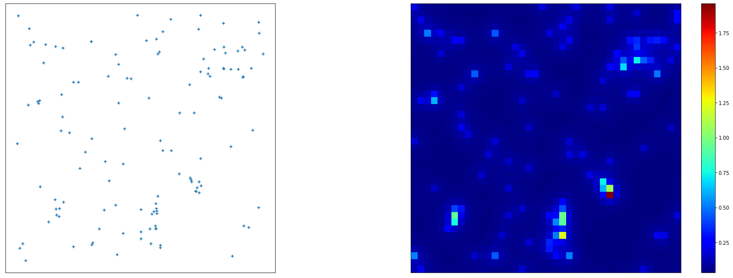
Refer to caption

Figure 11: Left: data points for the spatial point process example. Right: Inferred posterior rate for the Cox process with a 40×4040\times 40 discretization using AFT. The plot area is defined as having unit area. The samples were taken from a single run of AFT with 3030 temperatures and other parameters as discussed in the text.

We experimented with transforming the problem to a whitened representation x~\tilde{x} where x=L​x~+μx=L\tilde{x}+\mu and LL is the Cholesky decomposition of KK (Beskos et al., 2011; Neal, 2011). This can also be viewed as choosing a non-identity pre-conditioner or mass matrix. We found that this rendered the problem easier to the extent of no longer being a challenging benchmark, and that in this circumstance there was little that a NF could contribute. To maintain the difficulty of the baseline we therefore focused our comparison on the unwhitened space of the latent function.

The covariance KK is taken to be K⁡(u,v)=σ2​exp⁡(−‖u−v‖2M​β)K(u,v)=\sigma^{2}\exp\left(-\frac{||u-v||_{2}}{M\beta}\right), where σ2=1.91\sigma^{2}=1.91 and the mean vector has a constant value of log⁡(126)−σ2\log(126)-\sigma^{2}, and a=1/M2a=1/M^{2}, matching (Møller et al., 1998).

The Adam learning rate was 10−210^{-2} the training period JJ was 500500. AFT flow estimation particle numbers were Ntrain=Nval=2000N_{\textup{train}}=N_{\textup{val}}=2000.

For each transition, we used ten iterations of Hamiltonian Monte Carlo with 10 leapfrog steps per iteration. With the total time number of time steps scaled to be in the interval [0,1][0,1] with 00 being the initial distribution and 11 the final distribution, the slice sampling step sizes were interpolated between the times [0.,0.25,0.5,1.][0.,0.25,0.5,1.] using the step sizes [0.3,0.3,0.2,0.2][0.3,0.3,0.2,0.2]. The gold standard value for the normalizing constant shown in Figure 2 was found using 1000 repeats of SMC with 1000 temperatures and using the Cholesky whitening.

We found that to obtain best performance for AFT in this example, it was important to have sufficient HMC updates per transition.

An example of the samples produced using AFT can be seen in Figure 11.