Chronos: A general purpose classical AMG solver for High Performance Computing
Abstract
The numerical simulation of the physical systems has become in recent years a fundamental tool to perform analyses and predictions in several application fields, spanning from industry to the academy. As far as large scale simulations are concerned, one of the most computationally expensive task is the solution of linear systems arising from the discretization of the partial differential equations governing the physical processes. This work presents Chronos, a collection of linear algebra functions specifically designed for the solution of large, sparse linear systems on massively parallel computers (https://www.m3eweb.it/chronos/). Its emphasis is on modern, effective and scalable AMG preconditioners for High Performance Computing (HPC). This work describes the numerical algorithms and the main structures of this software suite, especially from the implementation standpoint. Several numerical results arising from practical mechanics and fluid dynamics applications with hundreds of millions of unknowns are addressed and compared with other state-of-the-art linear solvers, proving Chronos efficiency and robustness.
Keywords: parallel computing, HPC, preconditioning, algebraic mulgrid
1 Introduction
The solution of linear systems of equations is a central problem in a huge number of applications in both engineering and science. These problems are particularly crucial in the simulation of physical processes through the solution of partial differential equations or system of partial differential equations. In large-scale simulations, the solution of linear systems can be the most expensive task accounting for up to 99% of the total simulation cost.
In this work, we are interested in developing fast solution algorithms, suitable for High Performance Computers (HPC), for the linear system:
| (1) |
where is the system matrix, and are the right-hand side and solution vector, respectively, and is the number of equations. Although extension to general matrices is also possible, the present work restricts its focus to symmetric and positive definite (SPD) matrices which are very common in most mechanics and fluid dynamics applications.
In current industrial applications, can easily grow up to few hundreds of million of unknowns. On the other side, systems with billions of unknowns have also been solved in research experiments. The main difference between industrial problems and these huge research experiments is that the former are characterized by complex geometries, irregular discretizations and heterogeneities in the matrix coefficients, while the latter are generally obtained by successive refinements of regular or quite regular grids. Despite their smaller size, problems arising from real-world applications are very challenging and even having large computational resources may not be enough.
There are several methods to solve 1, both direct [33, 42, 2] and iterative [46, 18, 3], giving excellent performance on parallel computers. The former are generally preferred in industrial applications as they are typically more robust and require no experience from the user. The main downside is that, especially in 3D problems, the matrix factors require a huge amount of memory thus becoming the limiting factor for large scale simulations. This work is focused on iterative methods, more specifically on Algebraic Multigrid (AMG) preconditioning of iterative methods, because these latter present by far less memory restrictions and are suitable for almost perfectly parallel implementations. Moreover, in several practical cases, AMG preconditioning guarantees convergence in a number of iterations that does not depend or only slightly depends on the mesh size [49, 15, 53], a property of paramount importance for the extreme-size simulations that are foreseen in the near future. The main drawback of AMG preconditioning is that it is still far from being a black-box method, requiring an experienced user and sometimes a fine tuning of the set-up parameters. For most AMG solvers, a wrong set-up can easily lead to slow convergence or overly expensive preconditioners, and, in the worst cases, even to a failure in the solution [34]. AMG preconditioners can be divided into two principal families, classical AMG that are typically more effective on fluid dynamic problems and aggregation-based AMG which performs better in solid mechanics.
The Chronos package is a library of iterative methods and AMG preconditioners designed for high performance platforms to solve severely ill-conditioned problems arising in real-world industrial applications. To be effective on a wide range of different applications, Chronos allows for the choice of several options, from the adaptive generation of the operator near-kernel to the smoother selection, from coarsening to prolongation, all of this in the framework of the classical AMG method. In particular, it will be shown that BAMG interpolation makes this AMG extremely effective also on mechanical problems without the need to use an aggregation based coarsening. From the implementation standpoint, Chronos has been developed for HPC, adopting a distributed sparse matrix storage scheme where smaller CSR blocks are nested into a global CSR structure. This storage format, together with the adoption of non-blocking send/receive messages, allows for a high overlap between communications and computations thus hiding communication latency even for a relatively small amount of local operations. Finally, Chronos has a strongly object-oriented design to be readily linked to other software, to be used as an innermost kernel in more complex approaches, such as block preconditioners for multiphysics [1, 20, 22, 43, 52],and to be easily modified to support emerging hardware as GPU and FPGA [28, 26, 54].
The algorithms and methods presented in this work are not radically new, but are rather known algorithms revisited and highly tuned for challenging industrial problems from various fields. Particular care has been spent in the general design of the library in order to make it easily maintainable and amenable of improvements, without sacrificing performance. The benchmarks provided in the numerical experiments do not derive from the regular discretization of artificial problems, instead have been collected, also from other research/industrial groups, with the specific purpose of validating Chronos against the widest possible selection of test cases.
The remainder of the paper is organized as follows. In the next section, the classical AMG method will be briefly outlined with a large emphasis on the specific numerical algorithms implemented to increase effectiveness. In section 3, the design and structure of the library are accurately described especially from the implementation standpoint. The performance of Chronos is finally assessed in section 4 on a set of problems representative of a wide set of real world problems with a comparison with other state-of-the-art packages. The paper is closed with some concluding remarks and ideas for future work.
2 Classical Algebraic Multigrid framework
In this section, we briefly give an overview of classical AMG and describe, from a numerical viewpoint, all the AMG components and options, implemented in Chronos. One of the strengths of this library is that it offers several options for each AMG component to allow for the user to tune the best combination for any specific problem.
Any AMG method is generally built on three main components whose interplay gives the effectiveness of the overall method:
- •
Smoothing, where an inner preconditioner is applied to damp the high-frequency error components;
- •
Coarsening, in which coarse level variables are chosen for the construction of the next level;
- •
Interpolation, defining the transfer operator between coarse and fine variables.
In Chronos a fourth component, borrowed from the context of bootstrap and adaptive AMG [10, 12, 13, 14], is added to the above three and consists in a method to unveil hidden components of the near kernel of the linear operator whenever they are not a priori available.
As mentioned before, in the present work we are focused on the classical AMG setting, and below we will briefly recall the basic concepts behind this method, referring the interested reader to more detailed and rigorous descriptions in the works [48, 49, 53]. For the sake of clearness, we restrict this introduction to a two levels only scheme, as the multilevel version can be readily obtained by recursion.
The first component that has to be set-up in AMG is the smoother, which is a stationary iterative method responsible for eliminating the error components associated with large eigenvalues of , referred also as the high-frequency errors. The smoother is generally defined from a rough approximation of and its operator is represented by the following equation:
| (2) |
where is the identity matrix and a relaxation factor to ensure:
| (3) |
see for instance [21] for a short explanation. Generally, the smoother is given by a simple pointwise relaxation method such as (block) Jacobi or Gauss-Seidel, with the second one often preferred even though its use on parallel computers is not straightforward. Unlike other AMG packages such as BoomerAMG [27] or GAMG [6] where traditional smoothers like Gauss-Seidel or Chebyshev are selected by default, Chronos implements the adaptive Factorized Sparse Approximate Inverse (aFSAI) [30] so that the preconditioning matrix takes the following explicit form:
| (4) |
with lower triangular, so that its application simply requires two matrix-vector products. This choice is dictated by its almost perfect strong scalability and by its proven robustness in real engineering problems [4, 29]. Moreover, the cost of aFSAI application is usually much lower than that of Gauss-Seidel and Chebyshev since its density, i. e. the ratio between the number of non-zeroes of and , is generally .
The second component of AMG is the so-called Coarse-Grid Correction (CGC), which is the -orthogonal projection operation that should take care of the low-frequency components of the error. To build CGC in classical AMG, the unknowns of a given level are partitioned into Fine and Coarse (F/C), with those coarse variables becoming the unknowns of the next level. The choice of coarse variables is a crucial point in the AMG construction, as it determines both the rate at which the problem size is reduced and the convergence of the method. Here, we rely on the concept of Strenght of Connection (SoC), i.e., we associate to each edge of the adjacency graph of a measure of its relative importance. Then, using SoC, we rank the graph connections and filter out those deemed less important. A maximum independent set (MIS) is finally constructed on the filtered SoC graph to determine coarse variables.
To facilitate explanation, the system matrix is reordered according to this partitioning of the unknowns with first fine variables and second coarse ones:
| (5) |
with and square and matrices, respectively. Using this F/C ordering (5), the prolongation operator is written as:
| (6) |
where is a matrix containing the weights for coarse-to-fine variable interpolation. As the system matrix is SPD, the restriction operator is defined through a Galerkin approach as the transpose of , and the coarse level matrix is simply given by the triple matrix product:
| (7) |
In practice, fast convergence and rapid coarsening, i.e. high F/C ratios, are always desired, and the construction of effective prolongation operators is of paramount importance to conciliate these conflicting requirements.
Having defined all the above components, the set-up phase of the two-level multigrid method is completed and the iteration matrix is given by:
| (8) |
with and representing the number of smoothing steps performed before and after the coarse-grid correction, respectively.
Algorithms 1 and 2 briefly report the general AMG set-up phase and application in a V-cycle, respectively, in a multilevel framework, where it is conventionally assumed that , and . Details on all the computational kernels sketched in 1 and their parallel implementation will be discussed in the next sections/subsections.
2.1 Unveiling the operator near Kernel
The kernel (or null space) associated with the homogeneous discretized operator arising from the most common PDE or systems of PDE is generally a priori known. For instance it is well-known that the constant vector is the kernel for the Laplace operator and rigid body modes constitute the kernel for linear elasticity problems. The information needed to build these spaces, usually referred to as test spaces in the adaptive AMG terminology, is readily available to the user from nodal coordinates or other data retrievable from the discretization. However, the homogeneous operator kernel is only an approximation of the true near kernel associated with the fully assembled matrix and does not take into account all the peculiarities of the problem such as boundary conditions or the strong heterogeneities in the material properties that often arise in real-world problems. In many circumstances, a better test space can be obtained by simply modifying the initial near kernel suggested by the PDE. In the adaptive AMG literature [13, 14, 10, 35], the test space is found by simply running a few smoothing steps over a random test space or the initial near kernel, whenever available. However, since the near kernel of is related to the smallest eigenpairs of:
| (9) |
a better way to extract an effective test space could be by relying on an iterative eigensolver. In the present implementation, we opt for the simultaneous Rayleigh quotient minimization (SRQM) [8, 21] whose cost per iteration is only slightly higher than a smoothing step. By contrast, SRQM can provide a much better approximation of the smallest eigenpairs especially if a good preconditioner is provided. Since an approximation of is already available through the smoother, we simply reuse the previously computed inside the SRQM iteration.
From a theoretical standpoint, instead of solving (9), the test space should be computed by solving the generalized eigenproblem:
| (10) |
However, the SRQM solution to (10) needs the multiplication of by a vector which, due to our choice of (4), would result in a forward and backward triangular solve whose parallelization may represent an algorithmic bottleneck.
Unfortunately, extracting with high accuracy the eigenpairs of (9) is generally more expensive than solving the original linear system (1). For this reason, to limit the set-up cost, we only approximately solve (9) with a predetermined and small number of SRQM iterations. This simple strategy usually gives satisfactory results, whenever an initial test space is not available or boundary conditions and heterogeneity exert a strong influence, such as in geomechanical problems. Another appealing idea, though not explored in this work, is bootstrapping [10, 13, 14], which consists in computing a relatively cheap AMG preconditioner from a tentative test space, and then using AMG itself to better uncover the near null space and rebuild a more effective AMG. It will be shown in section 3 how the object-oriented implementation of Chronos allows for easily using such an approach through simple calls to high-level functions.
Operatively, once the test space is found, we compute an orthonormal basis of it and collect the basis vectors into a (skinny) matrix that may be subsequently used eventually for the strength of connection and the prolongation.
2.2 Strength of Connection
The construction of the coarse problem in
Chronos is based on the definition of a
SoC matrix, that is used to filter-out weak connections from the
adjacency graph of . There are three different SoC definitions available through
the library:
- 1.
Classical strength of connection:
(11) - 2.
Strength of connection based on strong couplings:
(12) - 3.
Affinity-based strength of connection:
(13)
where denotes the SoC between node and and and denote the entries in row and column of the matrices and , respectively. SoC (11) is particularly effective for Poisson-like problems where the system matrix is close to an M-matrix. SoC (12) is generally used in smoothed aggregation AMG [51] and usually gives good results in structural problems. Finally, SoC (13) has been introduced in [36] and, though requiring a rather expensive computation, it is able to accurately capture anisotropies as is shown in [41].
After SoC is computed for every pair of nodes, weak connections are eliminated to determine a Maximum Independent Set (MIS) of nodes that will become coarse nodes in the next level. The more aggressively the connections are eliminated, the higher number of nodes are left in the next level. There are two ways of controlling SoC filtering in Chronos:
- 1.
by a threshold, the traditional way of filtering, where we simply drop connections with strength below a given threshold ;
- 2.
prescribing an average number of connections per node.
On one side, guaranteeing an average number of connections per node is trickier, since it requires a preliminary sorting of all the SoC. On the other, it ensures a more regular grid coarsening through levels with an almost constant coarsening ratio. Moreover, in affinity-based SoC, the strength values usually lie in a narrow interval close to unity so that a proper choice of the drop threshold is almost impossible.
Finally, MIS construction is performed by using the PMIS strategy introduced in [17] which is a perfectly parallel algorithm giving generally rise to lower complexities than the classical Ruge-Stüben coarsening [16]. Using this more aggressive coarsening method requires some special care in the interpolation construction, as we will see in the next section.
2.3 Interpolation
Providing a good interpolation operator is crucial for an effective AMG method. We recall that the prolongation operator should satisfy:
| (14) |
where is the near-kernel of or, more precisely, for a coarse space of given size the optimal two-level prolongation as stated in [53, 11] should be such that:
| (15) |
where are the eigenvectors associated with the smallest eigenvalues of the generalized eigenproblem (10). To this aim, depending on the problem, we use two different strategies.
If a test space is available or it is relatively cheap to obtain a reasonable approximation of the near-kernel, then the so-called BAMG approach is used [10], where the weights of prolongation , i.e., the entries of the block in (6), are found through a least square minimization:
| (16) |
with the -th row of and the interpolatory set for . In practice, it is our experience that to have an effective prolongation, the norm must be reduced to zero and, in the general case, this can be accomplished only if the cardinality of , , is equal or larger than , the number of test vectors. To guarantee an exact interpolation, it is often necessary to use neighbors at a distance larger than one, especially when dealing with systems of PDEs, with a consequent increase of the overall operator complexity. Moreover, it may happen that, even if , some of the vectors are almost parallel and high conditioning of , the dense matrix defined below, may produce large jumps in the weights. In turn, large jumps in introduces high frequencies in the next level operator that the smoother hardly handles. To overcome these difficulties, we adopt an adaptive procedure to compute our BAMG interpolation. More in detail, let us define the matrix whose entries correspond to the -th component of the -th test vector , for any in the interpolatory set. For each fine node to be interpolated, we start by including in the interpolatory set all its coarse neighbors at a distance no larger than , and select a proper basis for by using a maxvol algorithm [32, 25]. If either the relative residual:
| (17) |
or the norm of the weights, , are larger than the user-defined thresholds and , respectively, then we extend by one the interpolation distance. We keep on increasing the interpolation distance up to to limit the computational cost. This procedure, which is briefly sketched in Algorithm 3, though slightly expensive, allows to compute an accurate and smooth prolongation without impacting too much on the operator complexity. In fact, including in all the coarse nodes within a priori selected interpolation distance usually leads to a more complex operator since several fine nodes may be interpolated with excessively large support. Moreover, limiting the number of non-zeroes in the rows of has the additional advantage that it is possible to perform prolongation smoothing without an exponential growth of the operator complexity. Prolongation smoothing is a very common practice in solving elasticity problems with aggregation-based AMG and numerical results will show how it can beneficial also in the context of classical AMG.
On the other hand, when there is no explicit knowledge of the test space or when the matrix at hand arises from the discretization of a Poisson-like problem, Chronos can also rely on more classical interpolation schemes. Below we briefly recall the expressions of some well-known interpolation formulas. First, using the concept of strength of connection, we define the following sets:
- •
, the set of direct neighbours of ;
- •
, the set of strongly connected neighbours of ;
- •
, the set of strongly connected fine neighbors of ;
- •
, the set of strongly connected coarse neighbors of ;
- •
, the set of weackly connected neighbors of .
A generally accurate distance-one interpolation formula, introduced in [44], is the classical interpolation. Unlike other distance-one formulas, here, the interpolation takes care of the contribution from strongly influencing points , and the expression for the interpolation weight is given by:
| (18) |
where:
| (19) |
It is worth noting that the original formula proposed in [44] is here corrected accordingly with the modification introduced in [27] where the set of strongly connected neighbors , that are F-points but do not have a common C-point, are subtracted to the fine strong neighbors . This modification of the interpolation formula is needed to avoid that the term vanishes. Indeed, using the PMIS-coarsening method no longer guarantees that two strongly connected F-points are interpolated by a common C-point. However, even if for a large class of problems the classical interpolation is very effective, it can lose efficiency for challenging problems such as rotated anisotropies or problems with large discontinuities. Indeed, in these cases, the convergence of the AMG accelerated by a Krylov subspace method can deteriorate, losing scalability and effectiveness. Hence, some more advanced interpolation formulas are required to overcome these difficulties. Particularly, we have to adopt some long-range interpolation strategies. A widely used interpolation strategy, mainly for very challenging Poisson-like problems, is the Extended+i interpolation. This interpolation formula is obtained extending the interpolatory set including C-points that are distance two away from the F-point we are considering. Furthermore, not only the connections from strong fine neighbors to points of the interpolatory set are considered, but also the connections from the fine neighbors to the fine point to be interpolated itself. Hence, denoting with the set of distance-two coarse nodes, the interpolation Extended plus i formula takes the following form:
| (20) |
with
| (21) |
This extended+i interpolation remedies many problems that occur with the distance-one interpolation formula and it provides better weight coefficients compared with other distance-two interpolation formulas. However, unlike the distance-one methods, they lead to much larger operator complexities. A possible way to reduce the complexities without or mildly affecting the convergence rate of the iterative scheme is to consider a different interpolatory set, i.e., an interpolatory set larger than the distance-one set , but smaller than the distance-two . The idea is to consider an interpolatory set that only extends for strong F-F connections without a common C-point, since in the other cases the point is already surrounded by interpolatory points belonging to . A crucial point is how to extend , ensuring as much as possible the quality of the interpolation operator. Here, we propose to enrich the set taking into account the minimum number of distance-two coarse nodes such as to guarantee that each F-F strong connection has at least a common C-point. To better explain this idea, let us consider the example in Figure 1.
Notice that using the classical interpolation, the interpolatory set would be and there would be two fine neighbors of , and , that do not share a C-point with . On the other hand, using the extended plus i interpolation, we would have that and each F-node, strongly connected with , would share at least one -node of the interpolatory set . However, to guarantee this last condition, it would be sufficient to only include the node to the set , so that the extended interpolatory set would become . It is worth noting that the new points included in the set are the minimum number of coarse point necessary to guarantee that each F-node strongly connected with the point to be interpolated, is also strongly connected with a C-node belonging to the interpolatory set. In other words, we extend the set by including the maximum independent set of distance-two C-nodes such that accomplish the above condition. Algorithms 4 gives a general description of the procedure used to make the extended interpolatory set.
2.4 Filtering
One problem that may affect AMG methods, especially in parallel implementation, is the excessive stencil growth occurring in lower levels. This drawback is even more pronounced if long-range interpolation or prolongation smoothing is used. Some authors have explored interesting solutions to reduce AMG complexity without detrimental effects on convergence [18, 9]. Simply eliminating small entries from the operators, as is done for instance with ILU or some approximate inverse preconditioners, may completely harm the effectiveness of CGC. This happens because removal of small entries from or may induce a representation of the near kernel of which is not accurate enough for AMG.
To overcome this problem, the authors in [18] propose to compensate the action of eliminated entries through a sort of stencil collapsing to guarantee that the filtered operator, say , exerts on the near kernel the same action of :
| (22) |
with a matrix representation of the near kernel. While it is relatively simple to enforce condition (22) for one dimensional near kernels, it is not immediate to accommodate the action on several vectors at the same time. With multiple vectors, first the smallest entries of are dropped to determine the pattern of , then a correction to , , is computed by using least squares on:
| (23) |
More in detail, is computed row-wisely such that the absolute norm of each row is a given percentage of the norm of the original one and then the compensation is computed for the same row. We use the same procedure on the prolongation operator with the only exception that instead of we use its injection in the coarse space. Operatively, the test space is used when available while in cases where is not computed, such as in Poisson problems, we simply replace with a unitary vector.
Finally, we observe that is no more guaranteed to be SPD and, especially when an aggressive dropping is enforced, the use of a non-symmetric Krylov solver, such as GMRES [45] or BiCGstab [50], is often needed instead of CG. Obviously, such care is not needed when only the prolongation is filtered as is always SPD for any choice of .
3 Library description
The Chronos software package is a collection of classes and functions that implements linear algebra algorithms for distributed memory parallel computers. The library is written in C++, and Message Passing Interface (MPI) and OpenMP directives were used for communication among processes and multithread execution, respectively. The hybrid MPI-OpenMP implementation is more flexible in the use of modern computing resources and it is generally more efficient than pure MPI due to its better exploitation of fine-grained parallelism.
Chronos has been developed using the potential of Object-Oriented Programming (OOP). The abstraction introduced through the OOP allows for using the same distributed matrix object to represent a linear system, a smoother, an AMG hierarchy or a preconditioner itself. Another advantage of this developed approach is the possibility to use simpler classes to derive more advanced elements, as block preconditioners. Moreover, whatever the type of preconditioner, the same iterative methods can be used for the linear system or eigenproblem solution.
In addition, the modular structure allows to easily integrate the CPU kernels with Graphics Processing Units (GPU) and Field Programmable Gate Array (FPGA) kernels leaving the overall architecture of the library unchanged, making Chronos a potentially multi-platform software. A hybrid CPU-GPU version is already under development and preliminary performances are encouraging [28].
A brief description of the main classes is reported in the next subsections.
3.1 Main classes
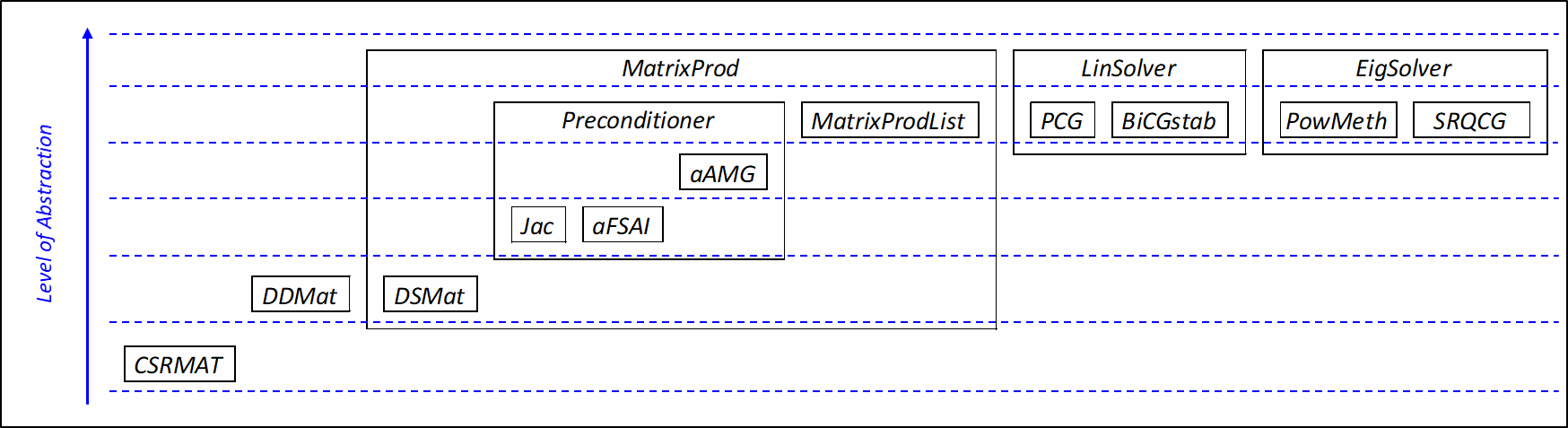
The level of abstraction and the hierarchy of the main classes are sketched in Figure 2. All these classes are exposed to the user to access the full range of Chronos functionalities.
The Distributed Dense Matrices (DDMat) and Distributed Sparse Matrices (DSMat) are managed by the and the classes, respectively. Both DDMat and DSMat storage schemes require the matrix to be subdivided into horizontal stripes of consecutive rows, where is the number of active MPI processes. In the DDMat, each stripe is stored row-wisely among the process to guarantee better access in memory during multiplication operations. This makes the DDMat very efficient for linear systems with multiple right-hand-sides and eigenproblems, and distributed vectors are stored as one-column DDMat. In the DSMat each stripe is subdivided into an array of Compact Sparse Row (CSR) matrices. The CSR format is the Chronos standard format for shared sparse matrices and their management is demanded to class. The DSMat storage scheme adopted in Chronos is very effective in both the preconditioner computation and the SpMV product because it allows a large superposition between communication and computation, and it is described in detail in the next subsection.
The class manages the approximation of the inverse of a Distributed Sparse Matrix at the highest level of abstraction. It requires in input a Distributed Sparse Matrix as -type object and an optional test space as a -type object. The classes derived from are , and that manage the preconditioners of Jacobian-type, adaptive-FSAI-type, and aAMG-type, respectively. A useful feature is that each of these classes can be used as a smoother in the AMG.
Both the and classes are derived from the class which manages the Sparse-Matrix-by-Vector product (SpMV) at the highest level of abstraction. The SpMV is the most expensive operation in any preconditioned iterative solver and its management has defined the design of the whole library. With reference to Figure 2, the class leads the Chronos structure together with the iterative solvers. Furthermore, more general elements can be readily built using the class, that manages an implicit object defined as a product of a sequence of objects ordered into a list.
At the top of the hierarchy pyramid, there are also the solvers for linear systems and eigenproblem, and , respectively. The manages the Krylov methods for linear system solution, it requires in an input preconditioner and a linear system as -type objects, a right-hand-side as a -type object and an optional initial solution as a -type object. The classes derived from are currently and that manage the Preconditioned Conjugate Gradient (PCG) iterative method and the Preconditioned Biconjugate Gradient Stabilized (BiCGstab) iterative method, respectively.
Finally, the manages the Krylov methods for the eigenproblem solution, it requires an optional input preconditioner and a linear system as -type objects and an initial eigenspace as a -type object. The two classes derived from are currently and , implementing the Power Method and the Simultaneous Rayleigh Quotient Minimization iterative methods, respectively.
3.2 Distributed Sparse Matrix Storage Scheme
The DSMat storage
scheme implemented in Chronos consists in partitioning
the matrix into horizontal stripes of consecutive rows.
Each stripe is then divided into blocks by applying the same subdivision to the
columns, as schematically shown in Figure 3, and each block is
stored as a CSR matrix.
The CSR matrices have a local numbering, i.e., rows and columns of block are numbered from 0 to and from 0 to , where and are the number of rows assigned to processes and , respectively. This expedient allows to use a 4-byte representation of integers, saving memory and increasing efficiency.
Each process stores only the diagonal block and the list of ”Left” (with a lower index) and ”Right” (with a higher index) blocks corresponding to the connections with neighboring processes. With reference to Figure 3, for instance, processor 3 stores the 5 blocks highlighted in red: 0, 1 and 2 as left neighbors, the diagonal block representing only internal connections and 6 as right neighbor.
This blocked scheme, although a bit cumbersome to implement, allows to stress non-blocking send/receive communications with a large superposition between communication and computation. It has proven to be very effective in all basic operations involving a DSMat: SpMV product, matrix-by-matrix product and matrix transposition.

4 Numerical results
The numerical experiments have been performed using large sparse matrices arising from the discretization of PDEs that model challenging real-world problems. The main goals of this section are basically to show the efficiency of the novel implementation of the Chronos package and to demonstrate its robustness and flexibility in dealing with severely ill-conditioned linear systems deriving form very different application fields, by switching the solution strategy through an appropriate parameter tuning. As described in the previous sections, the user can exploit the effectiveness of an advanced and tunable smoother like aFSAI, vary the coarsening ratio or switch between different interpolation methods depending on the specific problem at hand.
Chronos is benchmarked on a set of problems that can be grouped into two classes denoted as Fluid dynamic (F) and Mechanical (M). The first class of benchmarks consists of a series of problems arising from the discretization of the Laplace operator and related to fluid dynamic problems, such as underground fluid flow (reservoir), compressible or incompressible airflow around complex geometries (CFD) or porous flow (porous flow). The second category includes problems related to mechanical applications such as subsidence analysis, hydrocarbon recovery, gas storage (geomechanics), mesoscale simulation of composite materials (mesoscale), mechanical deformation of human tissues or organs subjected to medical interventions (biomedicine), design and analysis of mechanical elements, e.g., cutters, gears, air-coolers (mechanical).
In our experiments, we consider challenging test cases, not only for the high number of degrees of freedom (DOFs), but also because of their intrinsic ill-conditioning. Indeed, in real applications, we usually have to deal with severe jump of the physical proprieties, complicate geometries leading to highly distorted elements, heterogeneity and anisotropy. The matrices considered in the experiments are listed in Table 1 with details about the size, the number of non-zeros and the application field they arise from.
| Matrix | Class | avg. /row | Application field | ||
|---|---|---|---|---|---|
| finger4m | F | 4,718,592 | 23,591,424 | 5.00 | porous flow |
| guenda11m | M | 11,452,398 | 512,484,300 | 44.75 | geomechanics |
| agg14m | M | 14,106,408 | 633,142,730 | 44.88 | mesoscale |
| M20 | M | 20,056,050 | 1,634,926,088 | 81.52 | mechanical |
| tripod24m | M | 24,186,993 | 1,111,751,217 | 45.96 | mechanical |
| rtanis44m | F | 44,798,517 | 747,633,815 | 16.69 | porous flow |
| geo61m | M | 61,813,395 | 4,966,380,225 | 80.34 | geomechanics |
| poi65m | F | 65,939,264 | 460,595,552 | 6.99 | CFD |
| Pflow73m | F | 73,623,733 | 2,201,828,891 | 29.91 | reservoir |
| c4zz134m | M | 134,395,551 | 10,806,265,323 | 80.41 | biomedicine |
The reader can refer to Appendix A for a detailed description of each test case.
We subdivide the discussion of the results into two parts, the former collecting test cases from
fluid dynamics and the latter from mechanics. We also provide strong and weak scalability
analysis of the proposed implementation using large scale computational resources.
The result are presented in terms of total number of computational cores used ,
the grid and operator complexities, and , respectively, the number of
iteration to converge, and the set-up, iteration and total times, , and
, respectively.
The right-hand side vector used for all test cases is a random vector.
The linear systems are solved by the preconditioned conjugate gradient (PCG) method
with a zero initial solution and convergence is considered achieved when the
-norm of the iterative residual becomes smaller than .
The Chronos performance has been evaluated on the Marconi100 supercomputer,
from the Italian consortium for supercomputing (CINECA). Marconi100,
classified within the first ten positions of the TOP500 ranking [47] at the
time of writing, is composed by 980 nodes based on the IBM Power9 architecture, each
equipped with two 16-cores IBM POWER9 AC922 at 3.1 GHz processors.
For each test, the number of cores, , is selected to have a per core load
of about 100-150,000 unknowns and, consequently, different numbers of nodes are allocated
for different problem dimensions.
For all the tests, each node reserved for the run is always fully exploited. Furthermore,
in order to take advantage from the hybrid implementation and use also shared memory
parallelism, we always use 8 MPI tasks on each node and 4 OpenMP threads for each task.
As a reference point to evaluate the performance of Chronos, we compare it with the state-of-the-art solvers available from PETSc [6]. More specifically, we use BoomerAMG [27] and GAMG, the native PETSc aggregation-based AMG, as preconditioners in fluid dynamics and mechanical problems, respectively. The choice of BoomerAMG and GAMG as baseline solvers is because they are very well known and open-source packages whose performance have been demonstrated in several papers [15, 19, 27, 7].
4.1 Fluid dynamics test cases
The general purpose AMG implemented in Chronos is highly tunable offering several set-up options to effectively solve this set of problems as it will be shown below.
First, we start by comparing Chronos and BoomerAMG performance using as much as possible the same setup. Such comparison is intended to validate our HPC implementation and to demonstrate the efficiency of the DSMat storage scheme for SpMV product. To this purpose, we consider the three test cases finger4m, poi65m and Pflow73m. The comparison takes place with the same preconditioner configuration, i.e., Jacobi smoothing, classical SoC with , PMIS coarsening and extended+i prolongation. The first two rows of each test case reported in Table 2 provide the results obtained with this standard set-up. We denote by Chr-jac and Boomer-jac the Chronos and BoomerAMG preconditioners, both paired with Jacobi smoothing.
| Matrix | Solv. type | [s] | [s] | [s] | ||||
|---|---|---|---|---|---|---|---|---|
| finger4m | 32 | Chr-jac | 1.453 | 2.558 | 16 | 1.13 | 0.55 | 1.68 |
| 32 | Boomer-jac | 1.454 | 2.574 | 16 | 0.81 | 0.70 | 1.51 | |
| 32 | Chr | 1.453 | 2.558 | 7 | 3.71 | 0.33 | 4.04 | |
| 32 | Boomer | 1.454 | 2.574 | 12 | 0.79 | 0.94 | 1.73 | |
| poi65m | 384 | Chr-jac | 1.327 | 4.036 | 16 | 3.81 | 1.65 | 4.46 |
| 384 | Boomer-jac | 1.361 | 4.450 | 13 | 84.6 | 2.03 | 86.7 | |
| 384 | Chr | 1.346 | 4.496 | 6 | 27.5 | 1.84 | 29.34 | |
| 384 | Boomer | 1.361 | 4.450 | 14 | 80.2 | 3.18 | 83.4 | |
| Pflow73m | 480 | Chr-jac | 1.125 | 1.614 | 3308 | 14.1 | 611.9 | 626.0 |
| 480 | Boomer-jac | 1.123 | 1.593 | 3576 | 336.5 | 771.7 | 1108.2 | |
| 480 | Chr | 1.123 | 2.346 | 410 | 57.7 | 120.9 | 178.6 | |
| 480 | Boomer | 1.123 | 1.593 | 2777 | 340.5 | 1042.3 | 1382.8 |
First, we observe that the grid and operator complexities obtained with the two software
are basically the same and also the iteration count turns out to be quite similar, showing
that the two implementations are consistent. Only a slight difference occurs for
Pflow73m but we believe it is compatible with very small differences in the code
implementations.
Figure 4 provides the time spent for the preconditioner set-up (left)
and for the conjugate gradient iterations (right) for each solving strategy.
Each time reported in the figure is normalized with respect to the value obtained with
Boomer-jac, which is our baseline.
We can observe that Chronos is faster than BoomerAMG in the set-up for poi65m and
Pflow73m, while BoomerAMG is better in finger4m.
Differently, as far as the solving time is concerned, Chronos slightly outperforms
BoomerAMG in all the tests.
In all the cases tested, the SpMV and the Chronos implementation turns out to be
very efficient and the total solution time obtained is comparable and sometimes
even much better than those obtained with the BoomerAMG thanks to a faster set-up.
In Table 2 again, on the third and fourth rows, the labels Chr and Boomer identify the results obtained with Chronos and BoomerAMG when the default smoothers are selected, i.e., aFSAI and hybrid Gauss-Seidel, respectively. The use of a more evolute smoother with respect to either Jacobi or hybrid Gauss-Seidel gives a significant advantage in terms of iteration count and solving time at the price of a more expensive set-up, as shown in Table 2 and Figure 4. The use of the aFSAI always allows for achieving a faster convergence. Furthermore, the more ill-conditioned the problem is, the better aFSAI compares with other smoothers. In Pflow73m, which is the hardest problem in fluid dynamics, Chronos with aFSAI smoothing is 6 times faster than BoomerAMG. The set-up time is larger, but the speed-up obtained in the iteration stage may justify this effort, especially in transient simulations where the user may have to solve repeatedly the same linear system and can take advantage of preconditioner recycling.
In fluid dynamics, the prolongations of choice in combination with classical AMG are typically the classical or extended+i interpolations. This last is usually more effective, although more expensive, for changeling problems due to its ability to accurately interpolate also fine nodes having strong fine neighbors that do not share the same strong coarse node, possibly produced by high coarsening ratios. In Table 3, we compare these two well-known prolongations to the hybrid one that has been widely discussed in section 2.3.
| Matrix | Prol. type | [s] | [s] | [s] | ||||
|---|---|---|---|---|---|---|---|---|
| 32 | Chr-clas | 1.467 | 1.871 | 31 | 3.57 | 1.32 | 4.89 | |
| finger4m | 32 | Chr-hybc | 1.465 | 2.051 | 14 | 3.62 | 0.66 | 4.28 |
| 32 | Chr-exti | 1.453 | 2.558 | 7 | 3.71 | 0.33 | 4.04 | |
| 384 | Chr-clas | 1.612 | 1.943 | 46 | 23.3 | 6.47 | 29.8 | |
| rtanis44m | 384 | Chr-hybc | 1.585 | 2.030 | 36 | 26.6 | 6.09 | 32.8 |
| 384 | Chr-exti | 1.572 | 2.580 | 16 | 34.0 | 2.90 | 36.9 | |
| 384 | Chr-clas | 1.381 | 2.339 | 21 | 17.9 | 4.69 | 22.59 | |
| poi65m | 384 | Chr-hybc | 1.361 | 2.888 | 13 | 19.0 | 2.57 | 21.57 |
| 384 | Chr-exti | 1.346 | 4.496 | 6 | 27.5 | 1.84 | 29.34 | |
| 480 | Chr-clas | 1.236 | 1.391 | 414 | 39.4 | 60.2 | 99.6 | |
| Pflow73m | 480 | Chr-hybc | 1.234 | 1.448 | 416 | 40.4 | 67.1 | 107.5 |
| 480 | Chr-exti | 1.234 | 2.346 | 410 | 57.7 | 120.9 | 178.6 |
Let us consider first the results obtained for finger4m and poi65m for which the solver behavior is quite similar. We can observe that the extended+i interpolation is the more accurate one, with the higher value for operator complexity. As expected, this leads to a lower number of iterations, but a higher computational cost per iteration. On the contrary, the classical interpolation formula is the cheapest to compute, with a very low operator complexity. However, taking into account only distance-one coarse nodes, the prolongation operator is not able to efficiently reproduce the smooth error, causing an increase of the iteration count, up to twice the iteration count obtained with extended+i. For these two tests, the best configuration lies in the middle of these two, i.e., the hybrid interpolation formula, which keeps low the operator complexity taking into account just the distance-two coarse nodes actually useful to the interpolation process. In this way, we are able to obtain a more accurate interpolation formula with a computational cost comparable to the classical one.
The behavior is quite different for the other two test cases.
In rtanis44m, we have a strong heterogeneity and anisotropy of the permeability tensor,
factors that dramatically increase the problem ill-conditioning.
Hence, the most accurate interpolation method, i.e., extended+i, is needed to efficiently
solve this problem. The iteration count is one third with respect to classical interpolation
and the solution time is approximately one half.
Unlike before, the increased accuracy of the hybrid interpolation over classical is not enough
to give a sufficient benefit in terms of solving time.
It is worth noting that the increased set-up cost for extended+i is in this case largely
compensated in the iteration stage. This gain is even more pronounced in cases where
preconditioner recycling is possible such as in some transient or non-linear simulations.
The last test case considered in this section is Pflow73m, a very challenging and
severely ill-conditioned problem from underground flow.
Even if this is a diffusion problem, the great jumps in permeability and the distorted mesh
lead to a matrix whose near-kernel is not well represented by the unitary vector.
For this reason, the number of iterations required to achieve the convergence increases a lot
with respect to the other tests and not even the most accurate interpolations
such as extended+i or hybrid give any benefit over classical interpolation.
Hence, the cheapest classical formula proves also the most efficient strategy for this
test case.
4.2 Mechanical test cases
In this section, the potential of Chronos and its effectiveness in mechanical problems
are highlighted.
As seen above, Chronos allows for setting-up a very flexible AMG preconditioner,
adaptable to problem types the user has to solve, with different choices available
for interpolation operators and smoothing methods.
In addition, it allows the possibility to directly smooth the prolongation
and/or filter it.
As in the previous paragraph, we first define a baseline with
state-of-the-art methods such as BoomerAMG (Boomer), with Hybrid Gauss-Seidel smoothing,
the unknown-based Boomer with separate treatment of unknowns relative to different
directions (unk-based-Boomer) and the GAMG, an aggregation-based method.
We first refer to the test case tripod24m, whose results are provided in Table
4.
With the standard Boomer, the solution is reached with a high number of iterations,
more than 900 and the iteration time responsible of most of the total solution time.
A significant improvement is obtained using the unknown-based version [5],
where iterations are reduced by one third, and set-up and iteration times drop by 50%.
The aggregation based AMG seems to be the most effective one for mechanical problems as,
with GAMG, iterations are further reduced, and both and times decrease
significantly. In this problem, Chronos with BAMG prolongation and aFSAI smoother
(BAMG-aFSAI) is more effective than GAMG with a speed-up of two on the total time.
The set-up time is larger, but the number of PCG iterations is lower and the cost
per iteration is one-third of that of GAMG.
It is also possible to smooth the prolongation operator with Jacobi. We denote this
method as SBAMG-aFSAI. As could be expected, the operator complexity and the set-up
time both increase but, on the other hand, the number of iterations to converge and
the solution time are smaller.
Operator complexity and set-up time increases can be limited by means of filtering
(FBAMG-aFSAI) without compromising effectiveness. FBAMG-aFSAI requires the same number
of iterations to converge but at a lower cost per iteration.
These two last strategies are particularly effective in a FEM simulation where
the preconditioner can be reused several times in different time-steps so that the
set-up cost becomes secondary.
| Matrix | Prec. type | [s] | [s] | [s] | ||||
|---|---|---|---|---|---|---|---|---|
| Boomer | 1.244 | 3.207 | 931 | 64.1 | 611.9 | 676.1 | ||
| unk-based-Boomer | 1.328 | 3.669 | 335 | 43.8 | 262.4 | 203.5 | ||
| tripod24m | 160 | GAMG | 1.543 | - | 294 | 12.1 | 80.5 | 92.6 |
| BAMG-aFSAI | 1.041 | 1.116 | 222 | 21.8 | 23.0 | 44.8 | ||
| SBAMG-aFSAI | 1.041 | 1.322 | 118 | 36.7 | 16.1 | 52.9 | ||
| FBAMG-aFSAI | 1.041 | 1.212 | 120 | 33.5 | 13.5 | 47.0 |
Chronos proved robust and efficient in addressing all the mechanical test cases. A comparison of the number of iterations and times obtained with GAMG and the three BAMG strategies outlined above is shown in Table 5. To highlight the speed-up, Figure 5 shows set-up and the iteration time normalized to the GAMG times. Unfortunately, the comparison for the two largest cases, geo61m and c4zz13m, is not reported because these matrices have not been dumped on file due to their large size, and the tests have been run by linking Chronos to the FEM program ATLAS [24]. For the three benchmarks, guenda11m, tripod24m and M20, the number of PCG iterations required by GAMG and BAMG is comparable, but the overall solution time is significantly lower for BAMG with a speed-up of Chronos over GAMG up to 4 in these tests. The only exception is the matrix agg14m where GAMG is able to produce a very effective preconditioner at the lowest set-up cost.
Finally, with the aid of Figure 6, we would like to point out how the total solution time depends only mildly on the problem nature but on its size only. Figure 6 shows for each problem the total solution time divided by the number of non-zeroes per allocated core, and this resulting time is further normalized with the average among all the experiments. In other words, the figure should show the solution time for each problem as if exactly the same resources were allocated for each non-zero. For a preconditioner that is totally independent by the problem nature, it would be expected the same solution time for every problem. It can be observed that, through careful parameter tuning, Chronos is able to produce total solution times very close to the average normalized solution time, thus showing only a mild dependence on the application at hand.
| Matrix | Prol. type | [s] | [s] | [s] | ||||
|---|---|---|---|---|---|---|---|---|
| 64 | GAMG | 1.580 | - | 978 | 18.3 | 306.2 | 324.5 | |
| guenda11m | 64 | BAMG | 1.041 | 1.118 | 937 | 27.8 | 105.0 | 133.0 |
| 64 | SBAMG | 1.041 | 1.354 | 638 | 50.3 | 96.3 | 147.0 | |
| 64 | FBAMG | 1.041 | 1.240 | 638 | 43.5 | 79.8 | 123.0 | |
| 128 | GAMG | 1.644 | - | 26 | 12.5 | 5.8 | 18.2 | |
| agg14m | 128 | BAMG | 1.085 | 1.287 | 135 | 30.6 | 22.2 | 52.8 |
| 128 | SBAMG | 1.085 | 2.264 | 31 | 114.4 | 8.1 | 122.6 | |
| 128 | FBAMG | 1.085 | 1.670 | 34 | 53.6 | 7.3 | 60.9 | |
| 128 | GAMG | 1.162 | - | 245 | 211.0 | 391.4 | 602.4 | |
| M20 | 128 | BAMG | 1.054 | 1.184 | 775 | 71.2 | 275.0 | 347.0 |
| 128 | SBAMG | 1.054 | 1.677 | 151 | 158.0 | 71.2 | 229.2 | |
| 128 | FBAMG | 1.054 | 1.292 | 158 | 93.9 | 55.1 | 149.1 | |
| 160 | GAMG | 1.543 | - | 294 | 12.1 | 80.5 | 92.6 | |
| tripod24m | 160 | BAMG | 1.041 | 1.116 | 222 | 21.8 | 23.0 | 44.8 |
| 160 | SBAMG | 1.041 | 1.322 | 118 | 36.7 | 16.1 | 52.9 | |
| 160 | FBAMG | 1.041 | 1.212 | 120 | 33.5 | 13.5 | 47.0 |
4.3 Strong and weak scalability
In this last subsection, we evaluate the strong and weak scalability of the
AMG preconditioners implemented in Chronos.
All the three times, i. e. set-up , iteration and total times,
are analyzed to assess scalability.
The strong scalability test is shown in Figure 7, on the left
for the c4zz134m test matrix with BAMG prolongation and on the right for poi65m
with extended+i prolongation.
The number of cores varies from the minimum necessary to store matrix and preconditioner
up to 8 times the initial number. In both tests, the times decrease as the computing
resources increase, with a trend close to the ideal one.
Finally, the weak scaling is investigated with a standard 7-point finite difference discretization of the Poisson problem. Figure 8 shows, on the left, both the total time spent in the set-up and solve phase and, on the right, the parallel efficiency. Efficiency of weakly scaling up to nodes is defined as , with the time required on a single node and the time on nodes. In this test, we always assign 218,750 unknowns per core.
The result shows that efficiency is very good and keeps almost constant in the first two doubles of the cores, whereas a bit greater efficiency drop occurs in the last one. This performance dropdown can be ascribed to two different factors. First of all, while Marconi100 cores can be fully reserved for the test runs, the overall network is always shared with other users, and, consequently, the larger is the resource allocation, the larger the disturbance from other running processes. Secondly, a performance dropdown is almost unavoidable in AMG methods, as the grid hierarchy ends always up with small grids. The larger the number of resources allocated, the less efficient will be the software in dealing lower levels. Currently, to ease the implementation, Chronos uses all the allocated cores on each grid except the last one, where an allgather operation is called from a single core to solve the coarsest problem. In a future implementation, we plan to progressively reduce the amount of resources with levels, thus reducing the network traffic and increasing efficiency.
5 Conclusions
In this work, the Chronos library for the solution of large and sparse linear algebra problems on high performance platforms has been presented with a deep analysis of its numerical and computational performance. Chronos, which will be freely accessible to research institutions [23], provides iterative solution methods for linear systems and eigenproblems along with advanced parallel preconditioners.
Although the library comprises classical and novel methods already known in the literature, all of its algorithms have been attentively revisited, tuned and optimized on the basis of a large experimentation on real-world and industrial benchmarks arising from very different application fields. Moreover, every numerical kernel has been designed with special attention to its parallel performance and future extensibility to new numerical approaches and hardware.
The wide set of numerical experiments, provided in the work, clearly shows the ability of Chronos to give excellent performance in very different applications with solution times no worse or even better than those offered by other widely used HPC linear solvers as BoomerAMG and GAMG. Furthermore, this library offers great flexibility in the choice of the preconditioning strategy with the result that, once a proper set-up is found, total solution time depends solely or almost solely on the problem size and the number of computational resources allocated.
Our future work will be focused on porting Chronos on more energy-efficient and promising hardware such as GPU accelerators or FPGA, as well as using the innermost kernels of the library in developing advanced block preconditioners for multi-physics applications.
We also plan to build a stronger theoretical basis for the adaptive construction of the test space, unavoidable in problems lacking an initial guess for the operator near kernel, and for the operator and prolongation filtering which can greatly improve performance in though problems where denser operators may be needed.
Acknowledgments. The authors gratefully thank Proff. S. Koric, G. Mazzucco and E.L. Carniel, who provided the matrices M20, agg14m and c4zz134m used in the experiments.
Appendix A Description of the real-world applications
This appendix provides a detailed description of the test cases presented in this work, as listed in Table 1.
A.1 Test case finger4m
The matrix finger4m derives from a two-dimensional Darcy flow of a binary mixture. The physical model describes flow in a porous medium or Hele-Shaw cell, a thin gap between two parallel plates. The behavior of the system, and hence the matrix, is governed by two nondimensional groups: the Péclet number and the viscosity ratio [31].
A.2 Test cases guenda11m and geo61m
The matrices guenda11m and geo61m derive from two 3D geomechanical models of a reservoir.
In particular, the matrix guenda11m derives from a domain that spans an area of
and extends down to depth. To reproduce with high fidelity
the real geometry of the gas reservoir, a severely distorted mesh with linear
tetrahedra and vertices is used. While fixed boundaries are prescribed on the
bottom and lateral sides, the surface is traction-free.
The matrix geo61m represents a geological formation with 479 layers. The geometry of
the modeled domain is characterized by an area of with the reservoir
in an almost barycentric position and the base at a depth of . The grid is
based on a mesh of brick elements. The Figure 9 shows a
representation of the problem’s geometry and mesh. As can be observed, some elements are
highly distorted to reproduce the geological layers.

A.3 Test case agg14m
The mesh derives from a 3D mesoscale simulation of an heterogeneous cube of lightened concrete. The domain has dimensions and contains spherical inclusions of polystyrene. The cement matrix is characterized by , while the polystyrene inclusions are characterized by [37, 38]. Hence, the contrast between the Young modules of these two linear elastic materials is extremely high. The discretization is done via tetrahedral finite elements. The Figure 10 shows a representation of the problem’s geometry and mesh.

A.4 Test case M20
The mesh derives from the 3D mechanical equilibrium of a symmetric machine cutter that is loosely constrained. The unstructured mesh is composed by second order tetrahedra and vertices resulting in DOFs. Material is linear elastic with . This problem was initially presented by [34] and later used in the work [33].
A.5 Test case tripod24m
The mesh derives from the 3D mechanical equilibrium of a tripod with clamped bases. Material is linear elastic with . The mesh is formed by linear tetrahedra and discretization is given by the finite element method. Figure 11 shows the geometry and the mesh of the problem.

A.6 Test case rtanis44m
The mesh derives from a 3D diffusion problem in a porous media. The diffusion problem is governed by an anisotropic permeability tensor of the form , where is a rotation matrix and is a diagonal matrix defined as
with the rotation angle and the permeability matrix given by , , .
A.7 Test case poi65m
The mesh derives from the solution of the Poisson’s equation over a 3D cube. The domain is discretized with a finite difference grid.
A.8 Test case Pflow73m
The mesh derives from a basin model, with the discretization of a geological area - at the end of basin evolution - with a mesh of 20-node hexahedral elements. The Pflow73m matrix derives from the discretization of the mass conservation and Darcy’s law. Due to strong permeability contrasts between neighboring elements and geometrical distortion of the computational grid, the matrix is severely ill-conditioned and challenging to solve.
A.9 Test case c4zz134m
The mesh derives from the discrtization of the complex conformation of the urethral duct, with particular regard to the bulbar region. The duct locally consists of an inner thin layer of dense connective tissue and an outer thick stratum of more compliant spongy tissue [40, 39]. Both the materials are linear elastic, characterized by and , respectively. The Figure 12 shows a representation of the problem’s geometry and mesh.

References
- [1] F. P. Ali Beik and M. Benzi, Iterative Methods for Double Saddle Point Systems, SIAM Journal on Matrix Analysis and Applications, 39 (2018), pp. 902–921.
- [2] P. R. Amestoy, A. Buttari, J.-Y. L’Excellent, and T. Mary, Performance and Scalability of the Block Low-Rank Multifrontal Factorization on Multicore Architectures, ACM Transactions on Mathematical Software, 45 (2019), pp. 1–26.
- [3] S. Badia, A. F. Martín, and J. Principe, Multilevel balancing domain decomposition at extreme scales, SIAM Journal on Scientific Computing, 38 (2016), pp. C22–C52, https://doi.org/10.1137/15M1013511.
- [4] R. Baggio, A. Franceschini, N. Spiezia, and C. Janna, Rigid body modes deflation of the preconditioned conjugate gradient in the solution of discretized structural problems, Computers & Structures, 185 (2017), pp. 15–26, https://doi.org/10.1016/j.compstruc.2017.03.003.
- [5] A. H. Baker, T. V. Kolev, and U. M. Yang, Improving algebraic multigrid interpolation operators for linear elasticity problems, Numerical Linear Algebra with Applications, 17 (2009), pp. 495–517.
- [6] S. Balay, S. Abhyankar, M. F. Adams, J. Brown, P. Brune, K. Buschelman, L. Dalcin, A. Dener, V. Eijkhout, W. D. Gropp, D. Karpeyev, D. Kaushik, M. G. Knepley, D. A. May, L. C. McInnes, R. T. Mills, T. Munson, K. Rupp, P. Sanan, B. F. Smith, S. Zampini, H. Zhang, and H. Zhang, PETSc Web page. https://www.mcs.anl.gov/petsc, 2019, https://www.mcs.anl.gov/petsc.
- [7] S. Balay, S. Abhyankar, M. F. Adams, J. Brown, P. Brune, K. Buschelman, L. Dalcin, A. Dener, V. Eijkhout, W. D. Gropp, D. Karpeyev, D. Kaushik, M. G. Knepley, D. A. May, L. C. McInnes, R. T. Mills, T. Munson, K. Rupp, P. Sanan, B. F. Smith, S. Zampini, H. Zhang, and H. Zhang, PETSc users manual, Tech. Report ANL-95/11 - Revision 3.14, Argonne National Laboratory, 2020, https://www.mcs.anl.gov/petsc.
- [8] L. Bergamaschi, A. Martinez, and G. Pini, Parallel preconditioned conjugate gradient optimization of the Rayleigh quotient for the solution of sparse eigenproblems, Applied Mathematics and Computation, 175 (2006), pp. 1694–1715.
- [9] A. Bienz, R. D. Falgout, W. Gropp, L. N. Olson, and J. B. Schroder, Reducing Parallel Communication in Algebraic Multigrid through Sparsification, SIAM Journal on Scientific Computing, 38 (2016), pp. S332–S357.
- [10] A. Brandt, J. Brannick, K. Kahl, and I. Livshits, Bootstrap AMG, SIAM Journal on Scientific Computing, 33 (2011), pp. 612–632, https://doi.org/10.1137/090752973.
- [11] J. Brannick, F. Cao, K. Kahl, R. Falgout, and X. Hu, Optimal interpolation and compatible relaxation in classical algebraic multigrid, SIAM Journal on Scientific Computing, 40 (2018), pp. A1473–A1493, https://doi.org/10.1137/17M1123456.
- [12] M. Brezina, R. Falgout, S. MacLachlan, T. Manteuffel, S. McCormick, and J. Ruge, Adaptive smoothed aggregation (SA), SIAM Journal on Scientific Computing, 25 (2004), pp. 1896–1920, https://doi.org/10.1137/S1064827502418598.
- [13] M. Brezina, R. Falgout, S. MacLachlan, T. Manteuffel, S. McCormick, and J. Ruge, Adaptive smoothed aggregation (SA) multigrid, SIAM Review, 47 (2005), pp. 317–346, https://doi.org/10.1137/050626272.
- [14] M. Brezina, R. Falgout, S. MacLachlan, T. Manteuffel, S. McCormick, and J. Ruge, Adaptive algebraic multigrid, SIAM Journal on Scientific Computing, 27 (2006), pp. 1261–1286, https://doi.org/10.1137/040614402.
- [15] M. Brezina, C. Tong, and R. Becker, Parallel algebraic multigrids for structural mechanics, SIAM Journal on Scientific Computing, 27 (2006), pp. 1534–1554, https://doi.org/10.1137/040608271, https://doi.org/10.1137/040608271.
- [16] H. De Sterck, R. D. Falgout, J. W. Nolting, and U. M. Yang, Distance-two interpolation for parallel algebraic multigrid, Numerical Linear Algebra with Applications, 15 (2008), pp. 115–139.
- [17] H. De Sterck, U. M. Yang, and J. J. Heys, Reducing Complexity in Parallel Algebraic Multigrid Preconditioners, SIAM Journal on Matrix Analysis and Applications, 27 (2006), pp. 1019–1039.
- [18] R. D. Falgout and J. B. Schroder, Non-Galerkin Coarse Grids for Algebraic Multigrid, SIAM Journal on Scientific Computing, 36 (2014), pp. C309–C334.
- [19] R. D. Falgout and U. M. Yang, Hypre: A library of high performance preconditioners, in Proceedings of the International Conference on Computational Science-Part III, ICCS ’02, Berlin, Heidelberg, 2002, Springer-Verlag, pp. 632–641, http://dl.acm.org/citation.cfm?id=645459.653635.
- [20] M. Ferronato, A. Franceschini, C. Janna, N. Castelletto, and H. A. Tchelepi, A general preconditioning framework for coupled multiphysics problems with application to contact- and poro-mechanics, Journal of Computational Physics, 398 (2019), p. 108887.
- [21] A. Franceschini, V. A. Paludetto Magri, G. Mazzucco, N. Spiezia, and C. Janna, A robust adaptive algebraic multigrid linear solver for structural mechanics, Computer Methods in Applied Mechanics and Engineering, 352 (2019), pp. 389–416.
- [22] M. Frigo, N. Castelletto, and M. Ferronato, A Relaxed Physical Factorization Preconditioner for mixed finite element coupled poromechanics , SIAM J. Sci. Comput., 41 (2019), pp. B694–B720.
- [23] M. Frigo, G. Isotton, and C. Janna, Chronos Web page. https://www.m3eweb.it/chronos, 2020, https://www.m3eweb.it/chronos.
- [24] M. Frigo, G. Isotton, C. Janna, N. Spiezia, and O. Tosatto, ATLAS Web page. https://www.m3eweb.it/atlas, 2020, https://www.m3eweb.it/atlas.
- [25] S. A. Goreinov, I. V. Oseledets, D. Savostyanov, E. E. Tyrtyshnikov, and N. L. Zamarashkin, How to find a good submatrix, tech. report, Nov. 2008.
- [26] P. Haghi, T. Geng, A. Guo, T. Wang, and M. Herbordt, FP-AMG: FPGA-Based Acceleration Framework for Algebraic Multigrid Solvers, in 2020 IEEE 28th Annual International Symposium on Field-Programmable Custom Computing Machines (FCCM), IEEE, Apr. 2020, pp. 148–156.
- [27] V. E. Henson and U. M. Yang, BoomerAMG: A parallel algebraic multigrid solver and preconditioner, Applied Numerical Mathematics, 41 (2002), pp. 155 – 177, http://www.sciencedirect.com/science/article/pii/S0168927401001155. Developments and Trends in Iterative Methods for Large Systems of Equations - in memorium Rudiger Weiss.
- [28] G. Isotton, C. Janna, and M. Bernaschi, A gpu-accelerated adaptive fsai preconditioner for massively parallel simulations, International Journal for High Performance Computing Applications, (submitted).
- [29] C. Janna, M. Ferronato, and G. Gambolati, The use of supernodes in factored sparse approximate inverse preconditioning, SIAM Journal on Scientific Computing, 37 (2015), pp. C72–C94, https://doi.org/10.1137/140956026.
- [30] C. Janna, M. Ferronato, F. Sartoretto, and G. Gambolati, FSAIPACK: A software package for high-performance factored sparse approximate inverse preconditioning, ACM Trans. Math. Softw., 41 (2015), pp. 10:1–10:26, http://doi.acm.org/10.1145/2629475.
- [31] B. Jha, L. Cueto-Felgueroso, and R. Juanes, Fluid mixing from viscous fingering, Physical review letters, 106 (2011), p. 194502.
- [32] D. E. Knuth, Semi-optimal bases for linear dependencies, Linear and Multilinear Algebra, 17 (1985), pp. 1–4.
- [33] S. Koric and A. Gupta, Sparse matrix factorization in the implicit finite element method on petascale architecture, Comput. Methods Appl. Mech. Engrg., 302 (2016), pp. 281–292.
- [34] S. Koric, Q. Lu, and E. Guleryuz, Evaluation of massively parallel linear sparse solvers on unstructured finite element meshes, Computers & Structures, 141 (2014), pp. 19 – 25, https://doi.org/10.1016/j.compstruc.2014.05.009, https://doi.org/10.1016/j.compstruc.2014.05.009.
- [35] B. Lee, Algebraic multigrid for systems of elliptic boundary-value problems, Numerical Linear Algebra with Applications, 17 (2020), pp. 495–21.
- [36] O. E. Livne and A. Brandt, Lean algebraic multigrid (LAMG): Fast graph laplacian linear solver, SIAM Journal on Scientific Computing, 34 (2012), pp. B499–B522, https://doi.org/10.1137/110843563.
- [37] G. Mazzucco, B. Pomaro, V. Salomoni, and C. Majorana, Numerical modelling of ellipsoidal inclusions, Construction and Building Materials, 167 (2018), pp. 317–324.
- [38] G. Mazzucco, B. Pomaro, G. Xotta, C. E. Maiorana, and V. A. Salomoni, Tomography reconstruction of concrete materials for mesoscale modelling, Engineering Computations, (2020).
- [39] A. N. Natali, E. L. Carniel, C. G. Fontanella, A. Frigo, S. Todros, A. Rubini, G. M. De Benedictis, M. A. Cerruto, and W. Artibani, Mechanics of the urethral duct: tissue constitutive formulation and structural modeling for the investigation of lumen occlusion, Biomechanics and modeling in mechanobiology, 16 (2017), pp. 439–447.
- [40] A. N. Natali, E. L. Carniel, C. G. Fontanella, S. Todros, G. M. De Benedictis, M. A. Cerruto, and W. Artibani, Urethral lumen occlusion by artificial sphincteric devices: a computational biomechanics approach, Biomechanics and modeling in mechanobiology, 16 (2017), pp. 1439–1446.
- [41] V. A. Paludetto Magri, A. Franceschini, and C. Janna, A Novel Algebraic Multigrid Approach Based on Adaptive Smoothing and Prolongation for Ill-Conditioned Systems, SIAM Journal on Scientific Computing, 41 (2019), pp. A190–A219.
- [42] F.-H. Rouet, C. Ashcraft, J. Dawson, R. Grimes, E. Guleryuz, S. Koric, R. F. Lucas, J. S. Ong, T. A. Simons, and T.-T. Zhu, Scalability Challenges of an Industrial Implicit Finite Element Code, in 2020 IEEE International Parallel and Distributed Processing Symposium (IPDPS), IEEE, May 2020, pp. 505–514.
- [43] T. Roy, T. Jönsthövel, C. Lemon, and A. Wathen, A constrained pressure-temperature residual (cptr) method for non-isothermal multiphase flow in porous media, SIAM Journal on Scientific Computing, 42 (2020), pp. B1014–B1040.
- [44] J. W. Ruge and K. Stüben, Algebraic Multigrid, IEEE Educational Activities Department, 1987, ch. Society for Industrial and Applied Mathematics, pp. 73–130, http://locus.siam.org/doi/abs/10.1137/1.9781611971057.ch4.
- [45] Y. Saad and M. H. Schultz, GMRES: a generalized minimal residual algorithm for solving nonsymmetric linear systems, SIAM Journal on scientific and Statistical Computing, 7 (1986), pp. 856–869.
- [46] Y. Saad and H. A. Van der Vorst, Iterative solution of linear systems in the 20th century, Journal of Computational and Applied Mathematics, 123 (2000), pp. 1–33.
- [47] E. Strohmaier, J. Dongarra, H. Simon, and M. Meuer, Top500: The list of the 500 most powerful computer systems, 2020, https://www.top500.org.
- [48] K. Stüben, A review of algebraic multigrid, Journal of Computational and Applied Mathematics, 128 (2001), pp. 281 – 309, http://www.sciencedirect.com/science/article/pii/S0377042700005161. Numerical Analysis 2000. Vol. VII: Partial Differential Equations.
- [49] U. Trottenberg, C. Oosterlee, and A. Schüller, Multigrid, Academic Press, 2001, https://www.elsevier.com/books/multigrid/trottenberg/978-0-08-047956-9.
- [50] H. A. Van der Vorst, BI-CGSTAB: A fast and smoothly convergent variant of bi-cg for the solution of nonsymmetric linear systems, SIAM Journal on scientific and Statistical Computing, 13 (1992), pp. 631–664.
- [51] P. Vaněk, J. Mandel, and M. Brezina, Algebraic multigrid by smoothed aggregation for second and fourth order elliptic problems, Computing, 56 (1996), pp. 179–196, https://doi.org/10.1007/BF02238511.
- [52] M. Wathen and C. Greif, A Scalable Approximate Inverse Block Preconditioner for an Incompressible Magnetohydrodynamics Model Problem, SIAM Journal on Scientific Computing, 42 (2020), pp. B57–B79.
- [53] J. Xu and L. Zikatanov, Algebraic multigrid methods, Acta Numerica, 26 (2017), p. 591–721, http://dx.doi.org/10.1017/S0962492917000083.
- [54] O. Zachariadis, N. Satpute, J. Gómez-Luna, and J. Olivares, Accelerating sparse matrix–matrix multiplication with GPU Tensor Cores, Computers and Electrical Engineering, 88 (2020), p. 106848.