Data-Driven Retrospective Cost Adaptive Control
for Flight Control Applications
Abstract
Unlike fixed-gain robust control, which trades off performance with modeling uncertainty, direct adaptive control uses partial modeling information for online tuning. The present paper combines retrospective cost adaptive control (RCAC), a direct adaptive control technique for sampled-data systems, with online system identification based on recursive least squares (RLS) with variable-rate forgetting (VRF). The combination of RCAC and RLS-VRF constitutes data-driven RCAC (DDRCAC), where the online system identification is used to construct the target model, which defines the retrospective performance variable. This paper investigates the ability of RLS-VRF to provide the modeling information needed for the target model, especially nonminimum-phase (NMP) zeros. DDRCAC is applied to single-input, single-output (SISO) and multiple-input, multiple-output (MIMO) numerical examples with unknown NMP zeros, as well as several flight control problems, namely, unknown transition from minimum-phase to NMP lateral dynamics, flexible modes, flutter, and nonlinear planar missile dynamics.
1 Nomenclature
| = | performance-variable selection matrix |
| , , = | performance, control, and control-move weighting |
| FIA = | frozen input argument |
| = | identity matrix |
| = | step |
| = | fixed step with respect to |
| = | dimension of and |
| , , , = | dimensions of , , , |
| = | dimension of and |
| = | dimension of |
| = | controller window length |
| = | dimension of , , , , and |
| = | RCAC and DDRCAC tuning parameter |
| = | RLSID tuning parameter |
| = | disturbance and sensor noise covariance matrix for LQG design |
| = | state and control weight matrix for LQG design |
| = | dimension of and |
| = | forward-shift operator |
| = | proper, transfer functions |
| = | proper, discrete-time transfer functions |
| = | polynomial matrix in . |
| = | proper, discrete-time transfer function |
| , , = | , , |
| = | command |
| = | Laplace transform variable |
| = | sample time |
| = | time |
| = | control |
| = | sampled control |
| = | saturation level for RLSAC |
| = | sensor noise |
| vec = | column-stacking operator |
| = | sampled sensor noise |
| = | disturbance |
| = | constant disturbance during intersample subinterval |
| = | state |
| = | noisy measurement |
| = | noise-free system output |
| = | sampled noisy measurement |
| = | input vector of controller |
| = | noise-free sampled output due to and |
| = | performance variable |
| = | Z-transform variable |
| = | command-following error and adaptation variable |
| = | RLSID window length |
| = | controller coefficient vector |
| = | model coefficient vector |
| = | minimizer of RLS with VRF |
| = | RLSAC variable-rate forgetting factor |
| = | RLSID variable-rate forgetting factor |
| = | maximum singular value |
| = | denominator window length for VRF |
| = | numerator window length for VRF |
| = | Kronecker product |
| , , = | norm, norm, absolute value |
| = | set minus, set union |
| = | step function that is 0 for negative arguments and 1 otherwise |
| = | matrix of ’s |
2 Introduction
In direct adaptive control, the controller gains are updated in response to the actual dynamics of the controlled system. Unlike fixed-gain robust control, which trades off performance with prior modeling uncertainty, direct adaptive control uses partial modeling information for online self-tuning. Direct adaptive control is especially of interest for time-varying systems [1, 2]. The theory of direct adaptive control has been extensively developed [3, 4, 5, 6], and numerous successful applications to aerospace systems have been reported [7, 8]. The research challenge in direct adaptive control is to determine the minimal modeling information needed to facilitate fast, accurate, and reliable control.
As an alternative to direct adaptive control, indirect adaptive control performs online identification to update the required modeling information for use by a fixed-gain controller [4, pp. 397, 467], [5, chapter 7] . The combination of online identification and fixed-gain control is justified by the certainty equivalence principle [9, p. 2738]. Indirect adaptive control is advantageous for applications where the required modeling information is either difficult or impossible to obtain before operation due, for example, to unpredictable changes in the dynamics of the controlled system. By further reducing the dependence on prior modeling, indirect adaptive control facilitates control under extremely limited a priori modeling information. Indirect adaptive control can thus be viewed as a further step in the evolution of control from strong model dependence to model-free control.
Model-free control is a longstanding goal in control theory, and the challenges are far from trivial. In particular, data-driven control [10, 11] seeks to circumvent the need for a model using data. Furthermore, the interplay between identification and control is a longstanding problem in control theory [12, 13, 14]. This interplay is addressed by dual control, where the objective is to determine probing signals that enhance the speed and accuracy of the concurrent identification [15, 16, 17].
The present paper focuses on retrospective cost adaptive control (RCAC), which is a direct adaptive control technique for discrete-time and sampled-data systems [18, 19, 20]. The modeling information required by RCAC resides in the target model, which serves as an essential model of the closed-loop transfer function from the virtual external control perturbation to the retrospective performance variable. As shown in [20], the essential modeling information for discretized single-input, single-output (SISO) plants includes the sign of the leading numerator coefficient, the relative degree, and all nonminimum-phase (NMP) zeros. Numerical examples show that, under sufficiently aggressive tuning, RCAC may cancel unmodeled NMP zeros [21].
The goal of the present paper is to extend RCAC by incorporating online model identification; this method is called data-driven RCAC (DDRCAC). DDRCAC depends on system identification performed concurrently with controller adaptation, where the modeling details are extracted from the identified model in order to construct the target model. Since RCAC is based on recursive least squares (RLS) to update the controller coefficients, RLS is also used for system identification within DDRCAC. Unlike standard least squares, which uses constant-rate forgetting [22], online identification in the present paper takes advantage of RLS with variable-rate forgetting [23].
Note that DDRCAC uses online identification to obtain the modeling information needed by RCAC, which is a direct adaptive control technique. Consequently, DDRCAC is neither a direct adaptive control technique, which requires limited but precise modeling information, nor an indirect adaptive control, which requires modeling information in accordance with certainty equivalence. DDRCAC can thus be viewed is a hybrid direct/indirect adaptive control method that uses online system identification to obtain approximate, limited modeling information required by a direct adaptive control algorithm.
To assist in analyzing the effectiveness of DDRCAC and to obtain deeper insight into the modeling information required by the target model, the present paper shows that the retrospective performance variable can be decomposed into the sum of a performance term and a model-matching term. The performance term consists of a closed-loop transfer function, whereas the model-matching term involves the difference between a closed-loop transfer function and the target model driven by the virtual external control perturbation. A crucial insight arises from the observation that, at each step, RLS minimizes the magnitude of the retrospective performance variable by forcing the performance term and the model-matching term to have similar magnitudes but opposite signs. As the controller converges, the virtual external control perturbation, and thus the model-matching term, converges to zero, which, in turn, drives the performance term to zero. By preventing the performance term from diverging when the controller converges, this mechanism prevents RLS from converging to a controller that is destabilizing or has poor performance. The decomposition of the retrospective performance variable is used in this paper to elucidate the mechanism described above and diagnose the performance of DDRCAC.
As in all applications of system identification, persistency is needed to guarantee that the identified model captures the true system dynamics [24, 25, 26]. Persistency may be provided by the commands and disturbances, or it may be self-generated by the controller. Beyond persistency, since online identification and learning occur during closed-loop operation, the control input is correlated with the measurements due to disturbances and sensor noise. When RLS is used for closed-loop identification, as in the present article, this correlation may obstruct consistency, and thus lead to asymptotic bias in the parameter estimates [27, 28, 29]. Alternative identification methods, such as instrumental variables, provide consistency despite signal correlation, albeit at higher computational cost [30].
The present paper describes the elements of DDRCAC and investigates the effectiveness of this approach on numerical examples. These examples include synthetic examples that emphasize specific challenges as well as illustrative flight-control problems. The synthetic examples are focused on three key issues, namely, NMP zeros, consistency, and persistency. Since, as noted above, RCAC may cancel unmodeled NMP zeros, the highest priority is to extract information about the NMP zeros from the identified model; this information is embedded in the numerator of the identified model, which, in the case of a multiple-input, multiple-output (MIMO) system, is a matrix polynomial. These examples are motivated by the fact, as noted in [8], that the stability of finite transmission zeros is a standard assumption in output-feedback adaptive control. Furthermore, since lack of consistency may occur when RLS is used for closed-loop system identification, the effect of bias is examined. In particular, the bias arising from sensor noise within closed-loop system identification under DDRCAC is shown to be less severe than the bias arising from sensor noise within closed-loop system identification under fixed-gain control. Finally, in cases where the commands and disturbances provide limited persistency, these examples highlight self-generated persistency, that is, persistency due to the controller.
This paper applies DDRCAC to four flight-control examples. First, adaptive control is applied to roll-angle command following for a hypersonic aircraft that undergoes an unknown transition from minimum phase (MP) to NMP dynamics. Second, adaptive control is applied for pitch-rate command following of a flexible aircraft, which has 12 lightly damped modes. Third, adaptive control is applied for flutter suppression of the benchmark active control technology (BACT) wing Finally, adaptive control is applied to normal-acceleration command following for a nonlinear planar missile.
3 Sampled-Data Adaptive-Control Architecture
All of the examples in this paper consider continuous-time systems under sampled-data control using discrete-time adaptive controllers. In particular, consider the adaptive control architecture shown in Figure 1, where a realization of is given by
| (1) | ||||
| (2) |
where is the state, is the control, is the disturbance, is the noisy measurement of the system output, is the sensor noise, and are real matrices. Define
| (3) | ||||
| (4) |
where and are proper and transfer functions, respectively. The disturbance is matched if there exists such that ; otherwise, the disturbance is unmatched. The system output is corrupted by sensor noise and sampled to produce . The sampling operation can be realized as where is the sampled sensor noise and is the sample time. In this paper the statistics of the sampled sensor noise are specified. The performance variable is , where the matrix selects components of or a linear combination of the components of that are required to follow the command The command-following error is thus The inputs to the adaptive feedback controller are the measurement and the command-following error The adaptive feedback controller produces the discrete-time control at each step The continuous-time control is produced by applying a zero-order-hold operator to Note that serves as the adaptation variable, as denoted by the diagonal line in Figure 1 passing through The objective is to minimize the magnitude of the command-following error in the presence of the disturbance and sensor noise .
Figure 2 shows an equivalent representation of Figure 1, where and are related by the operator
| (5) |
Note that Figure 2 shows two transfer functions in feedback, namely, and , which are, respectively, the transfer functions from to and to . Furthermore, , where is the forward-shift operator, is the exact discretization of using zero-order-hold and sampling operations. For details, see [31, pp. 11]. Consequently,
| (6) | ||||
| (7) |
Note that the argument of in (6) reflects the fact that (6) is a time-domain equation whose solution depends on the initial conditions of the input-output system. Using the Z-transform variable in place of the forward-shift operator would account for the forced response of (6) but would implicitly assume zero initial conditions and thus would omit the free response. The distinction between and in accounting for initial conditions and the resulting free response is discussed in [32, 33]. Since and have the same form, the argument has no effect on the algebraic properties of such as poles and zeros.
In order to compute the intersample response of (5), the disturbance is assumed to be piecewise constant within each subinterval of the interval to where each subinterval has length In particular, letting denote the approximate value of for for it follows that
| (8) | ||||
| (9) | ||||
| (10) |
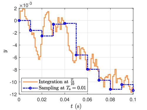
Within each subinterval, the MATLAB function ODE45 is used to integrate the dynamics of . For all examples in this paper, the ODE45 relative and absolute tolerances are set to and , respectively, which determine the variable step lengths during each subinterval. In the case where is stochastic, the standard deviation of is specified.
Figure 3 shows the intersample response of where is zero-mean, Gaussian white noise with standard deviation 1 simulated with s/step. In all subsequent numerical examples, the intersample response is computed but not shown.
Sections 4-6 consider SISO continuous-time transfer functions with of the form
| (11) |
where is a nonnegative integer, the parameters are given in Table 2, and and The transfer function (11) with the parameters in Table 2 are used to investigate the performance of RCAC, RLSID, and DDRCAC in later sections.
| Case | Zeros | ||||
|---|---|---|---|---|---|
| 1 real NMP | |||||
| 1 real NMP | |||||
| 2 complex NMP |
The time delay of , where is a nonnegative integer, is included in as . Choosing the time delay to be a multiple of facilitates investigation of the effect of uncertain discrete-time relative degree on the performance of the closed-loop discrete-time system. Note that (11) can be exactly discretized by separately considering the rational and exponential factors. In particular, the rational part of (11) is exactly discretized with a zero-order-hold (ZOH) discretization computed using MATLAB command c2d, whereas the exponential part of (11) is exactly discretized by the factor in . Note that the exact discretization of (11) has relative degree .
4 Retrospective Cost Adaptive Control
4.1 Controller Structure and Definition of the Retrospective Performance Variable
Consider the strictly proper, discrete-time dynamic compensator
| (12) |
where is the requested control, is the controller window length, , and and are the numerator and denominator controller coefficient matrices, respectively. For convenience, a “cold” startup is assumed, where , and are defined to be zero, and thus The controller (12) can be written as
| (13) |
where
is the controller regressor, and the controller coefficient vector is defined by
In terms of the controller (12) can be expressed as
| (21) |
where
| (22) | ||||
| (23) | ||||
| (24) |
The signal is constructed from and . In the simplest case, whereas, when additional measurements are available, Alternatively, feedforward action can be included by setting More generally, the components of can be arbitrary, fixed linear combinations of the components of and Fixed, nonlinear functions of and can also be included in ; however, this is outside the scope of this paper.
Next, define the filtered signals
| (25) | |||
| (26) |
where, for startup, and are initialized at zero and thus are computed as the forced responses of (161) and (162), respectively. Unless specified otherwise, the same filter initialization is for all filters in the subsequent development. The filter has the form
| (27) |
where
| (28) | ||||
| (29) |
is the filter window length, and and are the numerator and denominator coefficients of respectively.
Next, in order to update the controller coefficient vector (4.1), define the retrospective performance variable
| (46) |
where is given by (7) and is a generic variable for optimization. Note that depends on and thus on the current controller coefficient vector The retrospective performance variable is used to determine the updated controller coefficient vector by minimizing a function of The optimized value of is thus given by
| (47) |
which shows that the updated controller coefficient vector is “applied” retrospectively with the filtered controller regressor Furthermore, note that the filter is used to obtain from by means of (26) but ignores past changes in the controller coefficient vector, as can be seen by the product in (47). Consequently, the filtering used to construct (47) ignores changes in the controller coefficient vector over the window The effect of the actual time-dependence of is analyzed in later sections.
Using (30) and (31), (46) can be expressed as
| (48) |
In the case where is a finite-impulse-response (FIR) transfer function, and thus it follows from (48) that
| (49) |
In order to account for the control effort, define
where the performance weighting is nonsingular, and is the control weighting. If then all expressions involving in (4.1), as well as in all subsequent expressions, are omitted, and . Using (46), it follows that (4.1) can be expressed as
| (52) |
where
Using (4.1), define the retrospective cost
| (57) |
and note that
| (58) |
where is positive definite and is positive semidefinite. For all , the minimizer of (57) is given by the recursive least squares (RLS) solution [22]
| (59) | ||||
| (60) |
Using the updated controller coefficient vector given by (60), the requested control at step is given by
| (61) |
Although can be chosen arbitrarily, is chosen in all examples in order to reflect the absence of additional modeling information. Finally, , where is a tuning parameter.
4.2 Decomposition of the Retrospective Performance Variable
This subsection shows that the retrospective performance variable can be decomposed into the sum of a performance term and a model-matching term. A more restrictive version of the results in this section is given in [34]. For simplicity, this section focuses on the case where .
Since the optimized controller coefficient vector is time-dependent, the retrospective performance variable defined by (46) must be modified to ignore the time-dependence of . To do this, the terms in (46) are replaced by a filtered version of in which the controller coefficient vector is constrained to be over the filtering window. By defining
| (62) |
the filtered signal is given by a fixed-input-argument (FIA) filter with input as defined in Appendix B. In particular, is defined to be the output of the FIA filter
| (63) |
which ignores the change in the argument of over the interval in accordance with retrospective optimization. Note that, by the definition of FIA filtering, the filtered signal is a function of the time-dependent controller coefficient vector Equivalently, (63) can be written as
| (64) |
where
Using (63), the definition (46) of is replaced by
| (71) |
Using (62), (64), and (4.2), it follows that (71) can be written as
| (72) |
Note that the difference between given by (48) and given by (72) is due to the fact that in (48) is replaced by in (72). Hence, is not generally . However, if, for all then , and thus
The following result presents the retrospective performance-variable decomposition, which shows that the retrospective performance variable is a combination of the closed-loop performance and the extent to which the updated closed-loop transfer function from to matches the filter Henceforth, is called the target model since it serves as the target for the closed-loop transfer function from to .
Proposition 1
Assume that, for all and and are strictly proper. Then, for all
| (73) |
where the one-step predicted performance and the target-model matching performance are defined by
| (74) | ||||
| (75) |
and
| (76) | ||||
| (77) |
Proof. It follows from (74) and (76) that
| (78) |
Furthermore, defining the FIA filter output (see Definition 8.2 in Appendix B)
| (79) |
it follows from (77) and (79) that
| (80) |
Now, replacing with in (80) yields
| (81) |
Combining (78) and (79) yields
| (82) |
Next, replacing with in (62) and setting yields
| (83) |
Hence, using
it follows from (83) that
| (84) |
Using (22) and (23), note that (84) can be written as
which can be combined with (82) to obtain
| (85) |
Using (6) and (7), it follows from (85) that
| (86) |
which implies that
| (87) |
4.3 Analysis of the Retrospective Performance-Variable Decomposition
Assuming and using (4.1) and (73), it follows from (57) that
| (92) |
In the case where is large, using RLS to minimize (92) yields
| (93) |
Furthermore, it is observed numerically and shown in Figure 5 that using RLS to minimize (92) yields
| (94) |
which, using (73), implies that
| (95) |
that is,
| (96) |
The following example illustrates this property.
Example 4.1.
Minimization of and its decomposition for a SISO System. Let
| (97) |
and, for s/step, let denote the ZOH discretization of . Assume that the is matched, that is, and let be zero-mean, Gaussian white noise with standard deviation 1. For disturbance rejection with nonnoisy measurements, that is, with and adaptive control is applied with and . Figures 4(f) and (h) shows that, for all and have large magnitudes and approximately sum to zero. In particular, Figure 4(h) shows , which is small when and have large magnitudes with opposite signs, and close to when and have small magnitudes. Figure 4(g) shows that and have similar frequency responses, and thus the controller update promotes matching between the closed-loop transfer function and the target model .
Next, in order to compare and for the case where is IIR, the simulation is repeated with Figure 5 shows that the error between and is less than for all .


Proposition 1.
Assume that exists and is bounded. Then
Proof. Equations (4.1) and (62) imply that
Defining it follows that
where denotes the maximum singular value. Hence,
Proposition 1 and (75) suggest that the convergence of implies that converges to zero, as illustrated in Figure 4(g). Therefore, (96) implies that , and thus, if converges, then the one-step predicted performance is small. This mechanism underlies the convergence of RCAC in Figure 4 to a stabilizing controller that rejects the unknown disturbance. Note, however, that the convergence of and the consequent convergence of to zero do not imply that converges to zero. In fact, Example 4.5 demonstrates that a poor choice of may cause to diverge while converges.
4.4 Feasibility of
The following definition concerns the case where there exists a controller parameter vector that exactly matches the transfer function to .
Definition 4.1
Assume that, for all . Then, is feasible if there exists such that
| (98) |
where
| (99) |
with
| (100) | ||||
| (101) | ||||
| (102) |
Definition 4.1
For the SISO case, the following result identifies several features of that are determined by
Proposition 2.
For all assume that and are scalar. Furthermore, let and . Then the following statements hold:
- i)
The leading numerator coefficient of is equal to the leading numerator coefficient of
- ii)
The relative degree of is equal to the relative degree of
- iii)
The zeros of consist of the zeros of as well as zeros at zero.
Proof. Since and are scalar, it follows that is scalar and the closed-loop transfer function (99) specializes to
| (104) |
which implies i). To prove ii), let denote the degree of , and let denote the relative degree of , so that the degree of is . Since the degree of is and the degree of is it follows that the relative degree of is . Finally, iii) follows from the fact that the numerator of (104) is the numerator of multiplied by
The following result, which is an immediate consequence of Proposition 2, provides necessary conditions for feasibility in the SISO case.
Proposition 3.
For all assume that and are scalar. Furthermore, let , let , and assume that is feasible. Then the following statements hold:
-
The leading numerator coefficient of is equal to the leading numerator coefficient of .
-
The relative degree of is equal to the relative degree of .
-
The zeros of consist of the zeros of , as well as zeros at zero.
4.5 RCAC with Feasible and Infeasible for SISO Systems
This subsection investigates the effect of feasible and infeasible target models on the convergence of given by (60). For all of the examples in this and the following subsection, let be given by (97), and, for s/step, let denote the ZOH discretization of . In particular,
| (105) |
Assume that is matched, that is, and let and be zero-mean, Gaussian white noise with standard deviations 1 and 0.01, respectively. For various choices of the target model , the following examples consider disturbance rejection with noisy measurements with , and
Example 4.2.
Feasible . A linear-quadratic-Gaussian (LQG) controller is designed for given by (105) using the MATLAB command lqg with and The LQG controller
| (106) |
is used to construct
| (107) |
The corresponding closed-loop target model is given by
| (108) |
Note that (108) is feasible by construction. Since is feasible, Proposition 3 implies that its leading numerator coefficient and relative degree are the same as those of and that its zeros , and are the zeros of as well as zeros at zero. Next, adaptive control is applied with and . Figure 6(d) shows that and have similar frequency responses, which is consistent with the fact that is feasible. Moreover, Figure 6(b) shows that and have similar frequency responses, which suggests that the adaptive controller approximately converges to the LQG controller.

Example 4.3.
Robustness to infeasible . To investigate the robustness of the feasible target model (108), the target model is chosen to be various infeasible perturbations of the feasible target model given by
| (109) | ||||
| (110) | ||||
| (111) | ||||
| (112) |
which reflect uncertainty in and , respectively. Note that (109), (110), (111), and (112) are equal to (108) for the nominal values and respectively.
The suppression metric is defined as the ratio of the root-mean-square of the last 1000 subinterval steps of the open-loop response and the closed-loop response in dB. The case corresponds to disturbance suppression relative to the response of the open-loop system. Simulations where either or the output of the closed-loop system diverges are indicated as failures.
To investigate the closed-loop performance with an off-nominal target model, and are varied from their nominal values, and RCAC is applied with , for s. Figure 7 shows that the adaptive controller can be applied with the target models (109)–(112), where , , and are off-nominal. In particular, Figure 7 shows the suppression metric and asymptotic feasibility distance for target models with various sources of infeasibility. Figures 7(a) and 7(e) show and , respectively, for (109), where , which shows that infeasibility due to the sign of the leading numerator coefficient of the target model causes failure. However, the adaptive controller is robust to infeasibility due to the magnitude of the leading numerator coefficient of the target model. Figures 7(b) and 7(f) show and , respectively, for (110), where which shows that infeasibility due to the relative degree of target model causes failure. Figures 7(c) and 7(g) show and , respectively, for (111), where which shows that the adaptive controller is robust to infeasibility due to an incorrectly modeled MP zero in the target model. However, note that the adaptive controller fails when a MP zero of is replaced with a positive NMP zero in the target model. Figures 7(d) and 7(h) show and , respectively, for (112), where which shows that the adaptive controller is robust to infeasibility due to an incorrectly modeled NMP zero in the target model. Note that the adaptive controller fails when in the target model (112), that is, when the NMP zero in the feasible target model (108) is replaced with a MP zero.

4.6 Construction of for SISO Systems
Example 4.3 shows that RCAC can reject disturbances with an infeasible as long as shares certain properties with , as described by the following definition.
Definition 4.3
Assume that is SISO, and let be a proper SISO transfer function. Then is quasi-feasible if the following statements hold:
- i)
The leading numerator coefficients of and have the same sign.
- ii)
and have the same relative degree.
- iii)
and have the same NMP zeros.
Note that a quasi-feasible target model may be feasible; however, most quasi-feasible target model are infeasible
Definition 4.3
The nominal target model is the minimal-order, quasi-feasible FIR target model whose leading numerator coefficient is equal to the leading numerator coefficient of
Note that the nominal target model is uniquely defined. Furthermore, the nominal target model may be feasible; however, in most cases, the nominal target model is infeasible The rationale for choosing the nominal target model to be FIR is the fact that the target location for each closed-loop pole is the center of the open unit disk. For details, see [20]. Note that the nominal target model for , with given by (105), is
| (113) |
The following example investigates the efficacy of the nominal target model when the required modeling information is uncertain.
Example 4.4.
Robustness to perturbations from the nominal target model. To investigate the robustness of the nominal target model, first consider the case where given by (113). Figure 8 shows the suppression metric and the asymptotic feasibility distance for this choice of target model, marked with the vertical red dashed lines.
Next, the target model is chosen to be a perturbation of the nominal target model given by the off-nominal target models
| (114) | ||||
| (115) | ||||
| (116) |
which reflect uncertainty in and , respectively. Note that (114), (115), and (116) are equal to for the nominal values and respectively. To investigate the closed-loop performance with an off-nominal target model, and are varied from their nominal values, and adaptive control is applied with , for s. Figure 8 shows that the adaptive controller can be applied with the target models and , where and are off-nominal.

Example 4.4 suggests that can be constructed as
| (117) |
where are the leading numerator coefficient, all NMP zeros, number of NMP zeros, and relative degree of respectively. Note that the minus sign in (117) is due to the minus sign in (7).
Example 4.5.
Unmodeled NMP zeros and the retrospective performance-variable decomposition. Let which has the same leading numerator coefficient and relative degree as however, it does not have the NMP zero of Adaptive control is applied with and .
As shown by Examples 4.1 and 4.2, the minimization of the retrospective performance variable leads to matching between and Figure 9(h) shows that this is what happens for this example as well. Since (90) has a NMP zero at rad/step and does not, the optimization attempts to cancel this NMP zero using the denominator of (90). This results in a controller pole at the NMP zero as shown in Figure 9(g), which results in a hidden instability, demonstrated by the lack of divergence of and the exponential divergence of , as shown in Figures 9(e) and (a), respectively.
Additionally, as shown in Figure 9(b), the spectral radius of , which is the denominator polynomial of all closed-loop transfer functions, converges to a value greater than 1, which shows that all the closed-loop transfer functions are unstable. However, since is asymptotically stable, and and remain small, it follows from (71) that remains small, as shown in Figure 9(d). This in turn implies that , which can be seen in Figure 9(f).

4.7 MIMO Example
To investigate the role of the target model in MIMO case, note that the closed-loop transfer function from to is given by
| (118) | ||||
| (119) | ||||
| (120) |
asssume that and have full normal rank, and consider the definitions and propositions in Appendix A. Note that, if is square, then Proposition 5 implies that and are both empty. Alternatively, consider the case where , and thus in Figure 2 is rectangular. Note that both products and appear in (118)–(120). In particular, in the case where , is up-squared, and thus is empty, whereas is down-squared, and thus may be nonempty. On the other hand, in the case , is up-squared, and thus is empty, whereas is down-squared, and thus may be nonempty. As shown in the next example, cascade zeros of the down-squared loop transfer function may be cancelled by RCAC.
Example 4.6.
Cancellation of a NMP cascade zero. Consider and given by (3) and (4) with
and s/step. Note that is asymptotically stable. Let be a minimal realization of The objective is to reject the effect of a white, zero-mean, Gaussian disturbance on both components of and thus For (4.6), (4.6), has no transmission zeros and no NMP channel zeros. Let and be zero-mean, Gaussian white noise with standard deviations and , respectively. Using the Markov parameters and of , let
| (135) |
This choice of ensures that is not restricted to a subspace of , where , as shown in [35]. With given by (135) and , , , Figure 10 shows that a controller pole cancels a NMP cascade zero of at rad/step, which causes the control to diverge. Note that does not have a transmission zero at rad/step due to pole-zero cancellation, and thus the zero at rad/step is an evanescent NMP zero of .

5 Online Identification Using Recursive Least Squares
This section investigates the performance of RLS for online, closed-loop identification (RLSID). The goal is to estimate key features of the open-loop transfer function from to needed to construct , which, as shown in Section 4, serves as the target model for . Since closed-loop identification may lead to biased estimates, open-loop identification is also considered in order to provide a baseline comparison.
5.1 RLSID
In this subsection, RLSID is used to identify . The transfer function from to is given by
| (136) |
where , and are the numerator and denominator coefficients of the transfer function, respectively.
Consider the sampled-data identification architecture shown in Figure 11, which is based on Figure 2.
Since is known, can be computed internally by RLSID. Furthermore, at each step the requested control input and the measurement are assumed to be available. In order to identify , a model of the form
| (137) |
is fit to data where is the RLSID window length, and , and are numerator and denominator coefficient matrices that are to be estimated.
Next, note that (137) can be written as
| (138) |
where
| (145) |
is the model coefficient vector, and . The model-output error is defined by
| (146) |
where is an argument for optimization of the form
| (147) |
Next, to apply RLSID, note that the minimizer of the quadratic cost function
| (148) |
is given recursively by
| (149) | ||||
| (150) |
Note that is chosen to reflect the absence of additional modeling information, and , where is a tuning parameter. As shown by Example 5.1, the regularization term in (148), which is a required feature of RLS [36, 37, 38, 39], causes the estimates to be biased. Although the regularization-induced bias can be minimized by choosing to be large, it cannot be entirely avoided. The RLSID model at step is given by
| (151) |
Unless stated otherwise, for all of the examples in this paper RLSID is applied with a strictly proper model, which is enforced by removing and from the definitions (5.1) and (145), respectively, and redefining .
5.2 Relative Degree and Leading Numerator Coefficient of SISO Systems
In the case where and are scalar, the transfer function from to can be expressed as
| (152) |
where is the order of , and and are numerator and denominator coefficients, respectively. The leading numerator coefficient of (152) is the leftmost nonzero coefficient of , and the relative degree of (152) is Note that is leading numerator coefficient of , and, in the case where , .
5.3 Numerical Examples
For all of the examples in this section, let be given by Case 1 in Table 2, and let denote the ZOH discretization of with s/step, is a SISO 12th-order transfer function with a NMP zero at rad/step. Furthermore, and , and thus the relative degree of is and is its leading numerator coefficient. To assess the ability of RLSID to estimate the relative degree and leading numerator coefficient of , and are compared for Furthermore, to assess the accuracy of the estimate of the NMP zero of , the smallest distance between the zeros of the RLSID model and the NMP zero of is computed at each step. In order to assess the accuracy of open- and closed-loop identification, let , which is the order of Each example in this section involves 100 trials for s.
Example 5.1.
Open-loop RLSID with no disturbance, no sensor noise, showing regularization-induced bias. Let the input of be zero-mean, Gaussian white noise with standard deviation , and let and . To demonstrate the effect of regularization, RLSID is applied to the input-output data with two choices of namely, and , where and correspond to large and small regularization, respectively. A detailed treatment of regularization-induced bias in RLS is found in [40]. The averaged results from 100 trials are shown in Figure 12. As shown in Figure 12, the errors in the estimates of the first three numerator coefficients and the NMP zero are larger for trials with larger regularization.

Example 5.2.
Open-loop RLSID with disturbance and sensor noise. Let the input of be zero-mean, Gaussian white noise with standard deviation , let and To demonstrate the effect of disturbance and sensor noise, RLSID is applied to the input-output data with and with being zero-mean, Gaussian white noise with standard deviations respectively. The averaged results from 100 trials are shown in Figure 13. As shown in Figure 13, the errors in the estimates of the first three numerator coefficients and the NMP zero are larger for the trials with disturbance and sensor noise present.

Example 5.3.
Closed-loop RLSID with LQG Control. To demonstrate the effect of closed-loop control, RLSID is applied to the input-output data for open- and closed-loop scenarios. In particular, for open-loop simulations, is zero-mean, Gaussian white noise with standard deviation and for closed-loop simulations is given by an LQG feedback controller designed using the MATLAB command lqg with Let and be zero-mean, Gaussian white noise with standard deviations and , respectively. For RLSID set . The averaged results from 100 trials are shown in Figure 14. As shown in Figure 14, the errors in the estimates of the first three numerator coefficients and the NMP zero are larger for closed-loop input-output data relative to open-loop input-output data.

6 Data-Driven Retrospective Cost Adaptive Control
This section describes DDRCAC [41], which combines RLSID with RLS-based adaptive control (RLSAC). The online identification uses RLS to fit an infinite-impulse-response (IIR) model based on data and collected during closed-loop operation. At each step, the identified IIR model is used to construct a time-dependent target model . In particular, is constructed as an FIR filter whose numerator is chosen to be the numerator of the latest identified IIR model. Note that this online technique for constructing is a variation of the offline technique described in Section 4, where was constructed using only the NMP zeros of . This approach avoids the need to compute NMP zeros during online operation and can be used in the MIMO case, where the numerator of the RLSID model is a polynomial matrix. This target model is then used by RLSAC to update the coefficients of an IIR controller. For DDRCAC, both RLS implementations use variable-rate forgetting (VRF), as given by the following result [23].
Proposition 4.
For all , let , , and define Let , and let be positive definite. Furthermore, for all denote the minimizer of
| (153) |
where by Then, for all is given by
| (154) | ||||
| (155) |
For RLSID and RLSAC, a technique for specifying is given later in this section.
6.1 RLSID
In order to identify , an IIR model of the form (137) is fit to data. Since is known, can be computed internally by RLSID. Using Proposition 4, for all the model coefficient vector is updated recursively using
| (156) | ||||
| (157) |
where and are given by (5.1) and (145), respectively, and is positive definite. The RLSID model at step is given by
| (158) |
6.2 RLSAC
Define the strictly proper dynamic compensator
| (159) |
where and are given by (4.1) and (4.1), respectively. The definition (159) represents an IIR controller whose output is saturated component-wise by the scalar saturation function defined by
| (160) |
Next, define the filtered signals
| (161) | |||
| (162) |
where, for startup, and are initialized at zero and thus are computed as the forced responses of (161) and (162), respectively, and where is the time-dependent target model constructed using the updated numerator coefficients of the model (137). In particular,
| (163) |
which has the same form as (117) except that (163) is time varying, generalizes to MIMO systems, and includes all of the zeros of . In the case where , it follows from and that (163) and have the same leading numerator coefficient and relative degree. Note that, at each step the numerator of (163) is chosen to be the numerator of (158). If there exists such that then is chosen to be
| (164) |
The retrospective performance variable is defined to be
| (165) |
Using (163) and (164), (165) can be expressed as
| (166) |
where
| (167) |
and are given by (4.1) and (4.1) with , respectively, and are the numerator coefficients of the RLSID model. Note that, by performing the RLSID update at step before the RLSAC update, it follows thus the estimated numerator coefficients are available for constructing at step
Next, define the controller cost variable
where the performance weighting is nonsingular and , are the control weighting and control-move weighting, respectively. If and then and respectively, and all expressions involving and are omitted from (6.2), as well as from all subsequent expressions. Note that
| (171) |
where is positive definite, and , are positive semidefinite.
Using Proposition 4, for all the controller coefficient vector is updated recursively using
| (172) | ||||
| (173) |
where
and is positive definite.
For all of the examples in this paper, and are initialized as , and thus (164) is invoked at startup. This assumption reflects the absence of additional prior modeling information; however, and can be initialized based on any available modeling information. To initialize RLSAC and RLSID, and are chosen, where, for convenience, is a common tuning parameter.
6.3 Data-Dependent Variable Rate Forgetting
For data-dependent variable-rate forgetting, set
| (180) | ||||
| (181) |
where
| (182) |
“” is the step function that is 0 for negative arguments and 1 for nonnegative arguments, and In (180)–(182), , are numerator and denominator window lengths, respectively. If the sequence is zero-mean noise, then the numerator and denominator of (182) approximate the average standard deviation of the noise over the intervals and , respectively. In particular, by choosing , it follows that the denominator of (182) approximates the long-term-average standard deviation of whereas the numerator of (182) approximates the short-term-average standard deviation of Consequently, the case implies that the short-term-average standard deviation of is greater than the long-term-average standard deviation of plus a threshold of The function used in VRF suspends forgetting when the short-term-average standard deviation of drops below times the long-term-average standard deviation of This technique thus prevents forgetting in RLSID and RCAC due to zero-mean sensor noise with constant standard deviation rather than due to the magnitude of the noise-free identification error and command-following error.
A list of parameters to be selected for DDRCAC is presented in Table 3.
| Parameter | Description | Selection |
|---|---|---|
| Model window length | Integer (1–10) | |
| Controller window length | Integer (2–40) | |
| Control weighting | scaled identity | |
| Control move weighting | scaled identity | |
| Control saturation-limit vector | actuator saturation limit | |
| Initial RLS covariance scaling for RLSAC and RLSID | ||
| Forgetting parameter | (0.001 – 0.2) | |
| Forgetting window lengths | Integers ( [1–400], |
6.4 Numerical Examples
This subsection demonstrates DDRCAC, which uses no prior knowledge of and thus, in particular, no prior knowledge of the leading numerator coefficient, NMP zeros, or relative degree of Unless stated otherwise, all of the examples in this subsection use the same tuning parameters, namely, and Furthermore, for all of the examples in this section As in Section 5.3, the ability of RLSID to estimate the leading numerator coefficient and relative degree of is investigated by comparing the first numerator coefficients of the RLSID model and For all of the examples in this subsection RLSID and RLSAC are applied with a strictly proper RLSID model and target model, respectively, which is enforced by removing and from the definitions (5.1) and (145), respectively, redefining and
| (183) |
where .
Example 6.1.
Interaction between RLSID and RLSAC. Let
| (184) |
which is unstable and NMP, and, for s/step, let denote the ZOH discretization of . Then the NMP zero, leading numerator coefficient, and relative degree of are rad/step, and , respectively. Let , and let be zero-mean, Gaussian white noise with standard deviation .
For command following with control is applied using an LQG controller designed for augmented with a model of the harmonic command, using the MATLAB command lqg, with weights . Figures 15(a) and 15(c) show the response and control for the LQG controller, respectively. RLSID with VRF given by (156), (157) is used for closed-loop identification with the time-invariant LQG controller, as shown in Figures 15(e) and 15(h). In this case, the leading numerator coefficient and NMP zero of are estimated poorly, as shown by Figures 15(g),(h).
Next, adaptive control is applied with where Figures 15(k),(m) show that, at s, the leading numerator coefficient is correctly estimated, but the estimate of the NMP zero of is erroneous. The initially poor RLSID model at s results in a poor, infeasible target model, which induces a large transient response in and for s. The additional persistency of this transient response, however, facilitates subsequent identification of the NMP zero of at s, as shown in Figure 15(g). Note that is converged for s, and thus the time-dependent target model is also converged. With the converged time-dependent target model, Figure 15(g) shows that RLS with VRF facilitates further adaptation of for s, and is converged for s. This example thus illustrates mutually beneficial interaction between RLSID and RLSAC.

Example 6.2.
RCAC, DDRCAC, and decomposition. Let be given by Case 2 in Table 2 with s/step. In order to avoid numerical issues arising from the need for multiple discretized systems, the disturbance is assumed to be constant within each sampling interval Because is lightly damped, high-precision arithmetic is used to compare the left- and right-hand sides of (73).
For disturbance rejection, let , and let and be zero-mean, Gaussian white noise with standard deviations and , respectively. Three scenarios are considered, namely, (1) RCAC with the nominal target model which assumes knowledge of the true leading numerator coefficient, NMP zeros, and relative degree of (2) RCAC with the off-nominal target model where the leading numerator coefficient is erroneous by a factor of and the NMP zero is erroneous by a factor of , and (3) DDRCAC. RCAC is applied with , and which are identical to the tuning parameters for DDRCAC specified above.
The first, second, and third columns of Figure 16 correspond to scenarios (1), (2), and (3), respectively. Note that the closed-loop performance degrades significantly due to the use of the off-nominal target model. However, with no prior knowledge of the system dynamics, DDRCAC achieves closed-loop performance similar to RCAC with the nominal target model.
Figure 17 shows the RLSID coefficients , the true and estimated leading numerator coefficients and respectively, the variable-rate forgetting factors and the closest distance between the zeros of the RLSID model and the NMP zero of . Note that RLSID approximates the leading numerator coefficient, NMP zero, and relative degree of , and thus the time-dependent target model (163) approximates the nominal target model.


Example 6.3.
Effect of sensor noise and . Let be given by Case 3 in Table 2 with s/step. Then the NMP zeros, leading numerator coefficient, and relative degree of are rad/step, and , respectively. Hence, and The time-dependent target model (163) has the same leading numerator coefficient and relative degree as and is thus equal to the nominal target model, if and .
Let , let be Gaussian white noise with standard deviation and mean and consider three scenarios, where is zero-mean, Gaussian white noise with standard deviations and ; these scenarios correspond to the first, second, and third columns of Figure 18, respectively. The measurement signal-to-noise ratio (SNR) is defined to be the ratio of the root-mean-square of the last 1000 subinterval steps of to the root-mean-square of the last 1000 subinterval steps of . Note that the suppression metric decreases as SNR increases.
Next, to investigate the effect of three disturbance rejection scenarios with are considered, where is and ; these scenarios correspond to the first, second, and third columns of Figure 19, respectively. Note that, although the transient response of identified numerator coefficients increases with the level of asymptotic disturbance suppression is largely insensitive to the choice of


Example 6.4.
Example 4.6 revisited using DDRCAC. As shown in Example 4.6, the control of non-square MIMO systems using RCAC can cause the creation of NMP cascade zeros of that are cancelled by poles of leading to the divergence of DDRCAC is applied with , and thus the tuning parameters are identical to the RCAC tuning parameters in Example 4.6. As in Example 4.6, Figure 20 shows that the controller gives rise to NMP cascade zeros. However, unlike Example 4.6, these NMP zeros are not cancelled by the controller, and thus does not diverge.

Example 6.5.
Time-varying relative degree and NMP zeros with abrupt and smooth transitions. Let and be zero-mean, Gaussian white noise with standard deviations and , respectively, and Let , , and be given by Case 1, Case 2, and Case 3 in Table 2, respectively, with minimal realizations , , and , respectively. Furthermore, at each intersample time step let be given by (1) and (2) with
| (185) | |||
| (186) |
Note that, at s the relative degree of the discretization of (185) changes from to , and during s, the dynamics of of the discretization of (185) smoothly transition from a single real NMP zero at rad/step to a pair of complex NMP zeros at rad/step.
Figure 21 shows that the adaptive controller rejects the disturbance despite the unknown, abrupt and smooth transitions in the dynamics (185). Note that Figure 21(f), is equal to for s and equal to for s. Furthermore, note that are undefined for s, and are thus plotted for s in Figure 21(d).

7 Adaptive Flight Control
In this section, DDRCAC is applied to several flight-control problems, namely, (1) roll control of a hypersonic aircraft with an unknown transition from MP to NMP dynamics, (2) pitch-rate control of a flexible aircraft, (3) flutter suppression, and (4) normal-acceleration control a nonlinear planar missile. For consistency in applying DDRCAC, an exactly proper model structure used for RLSID for all of the examples in this section. Furthermore, the signal-to-noise ratio (SNR) between and is computed for all of the subinterval steps of each example. Note that the first three examples are linear, whereas the last example is nonlinear.
Example 7.1.
Roll control of a hypersonic aircraft with an unknown transition from MP to NMP dynamics. Consider the linearized lateral dynamics of a hypersonic aircraft [42, 43, 44], given by (1), (2) with
where the components of are sideslip angle in rad, body -axis angular velocity in rad/s, body -axis angular velocity in rad/s, and roll angle in rad, and the dynamics transition from MP to NMP. Note that, in the case of full-state feedback, that is, (7.1) and (7.1) possess no zeros and thus no NMP zeros. For this example, however, output feedback is assumed, and thus (7.1) and (7.1) may have NMP zeros. In addition, the measurements of the roll angle are assumed to be noisy. The roll-angle command is given by
| (199) |
which is a harmonic signal that abruptly changes frequency, followed by a sequence of step commands. The instantaneous poles and zeros of and as functions of are shown in Figures 22(a) and 22(b), respectively. The dynamics (7.1), (7.1) and their discretization transition from MP to NMP.

The signal represents the asymmetric deflection of the split flaps in rad. The actuator rate-saturation and magnitude-saturation limits are 300 deg/s and 30 deg, respectively. Let be Gaussian white noise with standard deviation and mean and let be zero-mean, Gaussian white noise with standard deviation . The onset, duration, and time-dependence of the transition from MP to NMP dynamics, which occurs during , are assumed to be unknown to the control algorithm.
Adaptive control is applied with , s/step, , and The response to the command (199) in the presence of disturbance is shown in Figure 23. By adapting to the unknown, changing dynamics in s, RLSID and RLSAC are able to follow commands.

Example 7.2.
Pitch-rate control of a flexible aircraft. Consider the pitch dynamics of a flexible aircraft [45] given by
| (200) |
where and This system represents a flexible aircraft cruising at Mach at ft, and includes aeroelastic effects. The transfer function (200) is lightly damped, asymptotically stable, and MP. This transfer function relates the elevator deflection in deg to the pitch rate measured at the cockpit in rad/s. The actuator rate-saturation and magnitude-saturation limits are 300 deg/s and 30 deg, respectively.
Assume that and let and be zero-mean, Gaussian white noise with standard deviations and respectively. The pitch-rate command is
| (201) |
For this example, the adaptive controller is configured for command feedforward by defining
Adaptive control is applied with s/step, and The response to a sequence of step commands in the presence of zero-mean, Gaussian white-noise disturbance is shown in Figure 24.

Example 7.3.
Flutter suppression. Consider the Benchmark Active Control Technology (BACT) for Active Control Design Applications [46, 47], which represents a wind-tunnel mounted wing that can translate vertically and pitch, and has a trailing edge flap as a control surface, as shown in Figure 25. Various control techniques have been used to demonstrate flutter suppression in BACT [48, 49, 50, 51, 52]. The BACT model incorporates a vertical spring and damper to model vertical aerodynamic forces, as well as a rotational spring and damper to model aerodynamic torques.

Accelerometers mounted on the leading and trailing edges of the wing measure the leading-edge normal acceleration and trailing-edge normal acceleration , respectively. The flutter-suppression objective is to drive and to using the control surface deflection , in the presence of turbulence. Second-order actuator dynamics and a second-order Dryden wind turbulence model are included in BACT. The disturbance represents the input to the second-order Dryden wind-turbulence model. BACT is an 8th-order, two-output-one-input, continuous-time, unstable, NMP, linear time-varying system with direct feedthrough, whose state-space matrices are functions of the freestream velocity For this example the freestream velocity is varied as
| (204) |
The onset, duration, and time-dependence of the change of freestream velocity, which occurs during , are assumed to be unknown to the control algorithm. The details of BACT are found in [47].
Let and be zero-mean, Gaussian white noise with standard deviations and , respectively. Adaptive control is applied with s/step, and The open- and closed-loop responses to a zero-mean, Gaussian white-noise disturbance are shown in Figure 26. As noted in Figure 26, the signal-to-noise ratio between the sampled noisy acceleration measurements and the sensor noise is approximately dB. Therefore, the root-mean-squared level of the sensor noise is approximately 23 as large as the root-mean-squared level of the acceleration measurements.

Example 7.4.
Normal-acceleration control of a nonlinear planar missile. Consider a tail-controlled interceptor missile, which is equipped with a strapdown accelerometer placed meters forward of the center of mass of the missile, where the distance is unknown. The missile [53, 54, 55] considered in this paper represents a missile in planar flight whose dynamics are given by
| (205) | ||||
| (206) | ||||
| (207) | ||||
| (208) | ||||
| (209) |
where arguments of are omitted for brevity, is the missile speed in is the thrust in N, is the acceleration due to gravity in is the angle of attack in rad, is the y-axis angular velocity in rad/s, is the flight-path angle in rad, is the altitude in m, is the applied fin angle in rad, is the dynamic force in N, is the air density in at an altitude m given by the Internal Standard Atmosphere model, is the reference surface area in , is the reference length in m, is the mass of the missile in kg, and is the moment of inertia of the missile relative to its center of mass and around a transverse axis in -. The angles and are shown in Figure 27. The values of the aerodynamic coefficients and parameter values are given in Tables 4 and 5, respectively.
| Aerodynamic Coefficient | Value | Units |
|---|---|---|
| - | ||
| - | ||
| - | ||
| - | ||
| - | ||
| s |
| Parameter | Value | Units |
|---|---|---|
| 204.0227 | kg | |
| 247.4366 | kg- | |
| 9.81 | ||
| 0.0409 | ||
| 0.2286 | m | |
| 1000 | N | |
| 0.5 | m |
Note that the aerodynamic coefficients are nonlinear functions of the missile speed , angle of attack and the local speed of sound , which depends on the altitude

The applied fin angle is related to the requested fin angle by means of second-order actuator dynamics with natural frequency rad/s, damping ratio , and magnitude and rate limits deg and deg/sec, respectively. The gravity-corrected normal acceleration measured by an accelerometer placed at a distance forward of the center of mass of the missile is given by
| (210) |
where and A noisy measurement of the normal acceleration , is used by the controller. The output equation (210) shows that there is a direct feedthrough of the applied fin to the normal acceleration used by the controller.
For this example, the adaptive controller is configured for command feedforward by defining
where the normal-acceleration command is . Let and be zero-mean, Gaussian white noise with standard deviations and respectively. Furthermore, let and Adaptive control is applied with s/step, , and The command-following response of the nonlinear planar missile is shown in Figure 28. After an initial transient, the command-following error is less than 5 g. Note that, starting with no prior knowledge of the nonlinear dynamics (205)–(209), the adaptive controller converges to a controller that facilitates command following.

8 Conclusions
In the presence of sensor noise and actuator magnitude and rate limits, DDRCAC was shown to be effective for plants with a priori unknown NMP zeros, in contrast with standard output-feedback adaptive control methods, which are confined to MP systems. DDRCAC was also shown to avoid cancellation of NMP squaring zeros, which are created due to the cascade of a nonsquare system and a controller. Using RLS with variable-rate forgetting, DDRCAC was found to provide self-generated persistency, thus facilitating system identification. Furthermore, although closed-loop identification can entail parameter-estimate bias, it was found that, in DDRCAC, identification and control interact so as reduce the effect of bias. Finally, flight-control examples showed that DDRCAC is effective for both linear and nonlinear applications as either a standalone embedded controller or as a simulation-based offline tuning technique for assessing achievable performance without requiring explicit knowledge of the underlying equations of motion.
Appendix A: Products of MIMO Transfer Functions and Pole-Zero Cancellations
This appendix considers pole-zero cancellation in products of MIMO transfer functions as these are present during control of MIMO systems.
Definition 8.0
Let . Then the normal rank of is defined by
| (213) |
Definition 8.0
Let be a realization of , where . Then the Rosenbrock system matrix of is the polynomial matrix
and is an invariant zero of if
| (216) |
If, in addition, is minimal, then is denoted by and is a transmission zero of if
| (217) |
Definition 8.0
Let be a realization of . Then IZ is the multiset of invariant zeros of , and TZ() is the multiset of transmission zeros of .
Definition 8.0
Let and with minimal realizations and , respectively. Define and consider its realization
Then is a cascade zero of if, counting repetitions, it is an invariant zero of (8.0) but not a transmission zero of either or The multiset of cascade zeros of is denoted by
| (223) |
Related results are found in [56, 57]. Squaring is discussed in [58, 59, 60] and used in [61] to eliminate NMP zeros. The following result shows that cascade zeros of square transfer functions exist only in the case .
Proposition 5.
Let and with minimal realizations and , respectively, where and , and assume that and have full normal rank. Define and consider its realization (8.0). If is not empty, then .
Proof. Suppose that , and let . Since is not a transmission zero of either or , has full column rank, and has full row rank, it follows from [62, Proposition 16.10.3] that
Next, note that
where
It follows from (Appendix A: Products of MIMO Transfer Functions and Pole-Zero Cancellations) and (Appendix A: Products of MIMO Transfer Functions and Pole-Zero Cancellations) that
| (237) |
Next, Sylvester’s inequality [62, p. 292, 294] implies
| (238) |
It follows from (Appendix A: Products of MIMO Transfer Functions and Pole-Zero Cancellations)–(238) that
| (239) |
which shows that there are no values of such that , and thus, , which is a contradiction.
Definition 8.0
Let and . Then the product is down squared if and up squared if .
Definition 8.0
Example 8.1.
Cascade and evanescent zeros. Consider the transfer functions
which have minimal realizations and , respectively, where
The Rosenbrock system matrices for and are
which show that and , and thus and are empty. Next, consider the product with the realization (8.0), which has the Rosenbrock system matrix
It can be shown that and . Since and are empty, it follows that and are elements of . Next, consider the product of the transfer functions in (8.1)
| (270) |
where the cascade zero at 3 is cancelled by a pole of , and thus is not an element off Therefore, is an element of .
Appendix B: Discrete-Time Filtering
This appendix reviews notation and terminology for discrete-time filtering in terms of the forward-shift operator . Define the proper discrete-time filter
| (271) |
where and are polynomial matrices and
Definition 8.1
The output of (271) with input is given by the data filter
| (272) |
Example 8.2.
Data filtering. Let and which yields the input-output difference equation
| (275) |
With the data and , (275) yields
| (276) | ||||
| (277) |
Definition 8.1 is now extended to the case where the input is a function of an independent variable .
Definition 8.2
Let let let be initial output data, let , and, for all let Then, the FIA sequence is given by the fixed-input-argument (FIA) filter
| (278) |
where, for all
Note that, at each step the arguments of in (278) are fixed at the current input value over the interval In contrast, the left-hand side defines the current output , which depends on the past output values For convenience, (278) is written as either
| (279) |
or
| (280) |
As a special case, note that
| (281) |
Example 8.3.
FIA filtering. Let and , and for all define
| (282) |
The corresponding FIA filter is thus given by
| (283) |
With the data , and , (283) yields
| (284) | ||||
| (285) |
Acknowledgments
The authors wish to thank John Burken and Tim Cox for providing the lateral aircraft dynamics model used in Example 7.1, Antai Xie for helpful discussions on the retrospective performance variable decomposition, Sneha Sanjeevini for discussions on the appendix, and Muneeza Azmat for discussions on filtering. This research was supported by ONR under BRC grant N00014-18-1-2211 and AFOSR under grant FA9550-20-1-0028 and DDDAS grant FA9550-18-1-0171.
References
- Parikh et al. [2019] Parikh, A., Kamalapurkar, R., and Dixon, W. E., “Integral Concurrent Learning: Adaptive Control with Parameter Convergence using Finite Excitation,” International Journal of Adaptive Control and Signal Processing, Vol. 33, No. 12, 2019, pp. 1775–1787. https://doi.org/10.1002/acs.2945.
- Gaudio et al. [2020] Gaudio, J. E., Annaswamy, A. M., Lavretsky, E., and Bolender, M. A., “Fast Parameter Convergence in Adaptive Flight Control,” AIAA Scitech, 2020. https://doi.org/10.2514/6.2020-0594, AIAA 2020-0594.
- Ioannou and Fidan [2006] Ioannou, P., and Fidan, B., Adaptive Control Tutorial, SIAM, 2006. https://doi.org/10.1137/1.9780898718652.
- Ioannou and Sun [2013] Ioannou, P., and Sun, J., Robust Adaptive Control, Dover, 2013. https://doi.org/10.1007/978-1-4471-5102-9_118-1.
- Tao [2003] Tao, G., Adaptive Control Design and Analysis, Wiley, 2003. https://doi.org/10.1002/0471459100.
- Ilchmann [1991] Ilchmann, A., “Non-Identifier-Based Adaptive Control of Dynamical Systems: A Survey,” IMA Journal of Mathematical Control and Information, Vol. 8, 1991, pp. 321–366. https://doi.org/10.1093/imamci/8.4.321.
- Hovakimyan et al. [2011] Hovakimyan, N., Cao, C., Kharisov, E., Xargay, E., and Gregory, I. M., “L1 Adaptive Control for Safety-Critical Systems,” IEEE Control Systems Magazine, Vol. 31, No. 5, 2011, pp. 54–104. https://doi.org/10.1109/MCS.2011.941961.
- Wiese et al. [2015] Wiese, D. P., Annaswamy, A. M., Muse, J. A., Bolender, M. A., and Lavretsky, E., “Adaptive Output Feedback Based on Closed-Loop Reference Models for Hypersonic Vehicles,” AIAA Journal of Guidance, Control, and Dynamics, Vol. 38, No. 12, 2015, pp. 2429–2440. https://doi.org/10.2514/1.G001098.
- Tao [2014] Tao, G., “Multivariable adaptive control: A survey,” Automatica, Vol. 50, No. 11, 2014, pp. 2737–2764. https://doi.org/10.1016/j.automatica.2014.10.015.
- Hou and Wang [2013] Hou, Z.-S., and Wang, Z., “From model-based control to data-driven control: Survey, classification and perspective,” Information Sciences, Vol. 235, 2013, pp. 3–35. https://doi.org/10.1016/j.ins.2012.07.014.
- Gao et al. [2017] Gao, W., Jiang, Z., and Ozbay, K., “Data-Driven Adaptive Optimal Control of Connected Vehicles,” IEEE Transactions on Intelligent Transportation Systems, Vol. 18, No. 5, 2017, pp. 1122–1133. https://doi.org/10.1109/TITS.2016.2597279.
- den Hof and Schrama [1995] den Hof, P. V., and Schrama, R. J. P., “Identification and control — Closed-loop Issues,” Automatica, Vol. 31, No. 12, 1995, pp. 1751–1770. https://doi.org/10.1016/0005-1098(95)00094-X.
- Gevers [1993] Gevers, M., “Towards a Joint Design of Identification and Control?” Progress in Systems and Control Theory, Vol. 14, 1993, pp. 111––151. https://doi.org/10.1007/978-1-4612-0313-1_5.
- Hjalmarsson [2005] Hjalmarsson, H., “From Experiment Design to Closed-Loop Control,” Automatica, Vol. 41, No. 3, 2005, pp. 393–438. https://doi.org/10.1016/j.automatica.2004.11.021.
- Feldbaum [1961] Feldbaum, A. A., “Dual Control Theory,” Avtomatika i Telemekhanika, Vol. 22, No. 1, 1961, pp. 3–16.
- Wittenmark [1995] Wittenmark, B., “Adaptive Dual Control Methods: An Overview,” Adaptive Systems in Control and Signal Processing, Vol. 28, 1995, pp. 67–72. https://doi.org/10.1016/B978-0-08-042375-3.50010-X.
- Filatov and Unbehauen [2004] Filatov, N. M., and Unbehauen, H., Adaptive Dual Control: Theory and Applications, Springer, 2004. https://doi.org/10.1007/b96083.
- Santillo and Bernstein [2010] Santillo, M. A., and Bernstein, D. S., “Adaptive Control Based on Retrospective Cost Optimization,” AIAA Journal of Guidance, Control, and Dynamics, Vol. 33, No. 2, 2010, pp. 289–304. https://doi.org/10.2514/1.46741.
- Hoagg and Bernstein [2012] Hoagg, J. B., and Bernstein, D. S., “Retrospective Cost Model Reference Adaptive Control for Nonminimum-Phase Systems,” AIAA Journal of Guidance, Control, and Dynamics, Vol. 35, 2012, pp. 1767–1786. https://doi.org/10.2514/1.57001.
- Rahman et al. [2017] Rahman, Y., Xie, A., and Bernstein, D. S., “Retrospective Cost Adaptive Control: Pole Placement, Frequency Response, and Connections with LQG Control,” IEEE Control Systems Magazine, Vol. 37, 2017, pp. 28–69. https://doi.org/10.1109/MCS.2017.2718825.
- Islam et al. [2019] Islam, S. A. U., Xie, A., and Bernstein, D. S., “Adaptive Control of Systems with Unknown Nonminimum-Phase Zeros Using Cancellation-Based Pseudo-identification,” Proceedings of the American Control Conference, Philadelphia, PA, 2019, pp. 441–446. https://doi.org/10.23919/ACC.2019.8814620.
- Islam and Bernstein [2019] Islam, S. A. U., and Bernstein, D. S., “Recursive Least Squares for Real-Time Implementation,” IEEE Control Systems Magazine, Vol. 39, No. 3, 2019, pp. 82–85. https://doi.org/10.1109/MCS.2019.2900788.
- Bruce et al. [2020] Bruce, A. L., Goel, A., and Bernstein, D. S., “ Convergence and Consistency of Recursive Least Squares with Variable-Rate Forgetting,” Automatica, Vol. 119, 2020, p. 109052. https://doi.org/10.1016/j.automatica.2020.109052.
- Willems et al. [2005] Willems, J. C., Rapisarda, P., Markovsky, I., and De Moor, B. L. M., “ A Note on Persistency of Excitation ,” Systems and Control Letters, Vol. 77, No. 4, 2005, pp. 325–329. https://doi.org/10.1016/j.sysconle.2004.09.003.
- Goel et al. [2020] Goel, A., Bruce, A., and Bernstein, D. S., “Recursive Least Squares with Variable-Direction Forgetting: Compensating for the Loss of Persistency,” IEEE Control Systems Magazine, Vol. 40, 2020, pp. 80–102. https://doi.org/10.1109/MCS.2020.2990516.
- Chowdhary et al. [2014] Chowdhary, G., Mühlegg, M., and Johnson, E. N., “Exponential Parameter and Tracking Error Convergence Guarantees for Adaptive Controllers without Persistency of Excitation,” International Journal of Control, Vol. 87, No. 8, 2014, pp. 1583–1603. https://doi.org/10.1080/00207179.2014.880128.
- Forssell and Ljung [1999] Forssell, U., and Ljung, L., “Closed-Loop Identification Revisited,” Automatica, Vol. 35, No. 7, 1999, pp. 1215–1241. https://doi.org/10.1016/S0005-1098(99)00022-9.
- Aljanaideh and Bernstein [2017] Aljanaideh, K. F., and Bernstein, D. S., “Closed-Loop Identification of Unstable Systems Using Noncausal FIR Models,” International Journal of Control, Vol. 90, No. 2, 2017, pp. 168–185. https://doi.org/10.1080/00207179.2016.1172733.
- Sobolic et al. [2020] Sobolic, F., Aljanaideh, K. F., and Bernstein, D. S., “A Numerical Investigation of Direct and Indirect Closed-Loop Architectures for Estimating Nonminimum-Phase Zeros,” International Journal of Control, Vol. 93, No. 6, 2020, pp. 1251–1265. https://doi.org/10.1080/00207179.2018.1501609.
- Gilson and den Hof [2005] Gilson, M., and den Hof, P. V., “Instrumental Variable Methods for Closed-loop System Identification,” Automatica, Vol. 41, No. 7, 2005, pp. 241–249. https://doi.org/10.1016/j.automatica.2004.09.016.
- Chen et al. [1995] Chen, T., Tapn, T., and Francis, B., Optimal Sampled-Data Control Systems, Springer, 1995. https://doi.org/10.1007/978-1-4471-3037-6.
- Aljanaideh and Bernstein [2018] Aljanaideh, K. F., and Bernstein, D. S., “Initial Conditions in Time- and Frequency-Domain System Identification: Implications of the Shift Operator Versus the Z and Discrete Fourier Transforms,” IEEE Control Systems Magazine, Vol. 38, No. 2, 2018, pp. 80–93. https://doi.org/10.1109/MCS.2017.2786419.
- Middleton and Goodwin [1990] Middleton, R., and Goodwin, G., Digital Control and Estimation: A Unified Approach, Prentice Hall, 1990. https://doi.org/10.1002/rnc.4590040308.
- Islam et al. [2021] Islam, S. A. U., Xie, A., and Bernstein, D. S., “Closed-Loop Performance versus Target-Model Matching in Retrospective Cost Adaptive Control,” Proceedings of the American Control Conference, New Orleans, LA, 2021. to appear.
- Goel and Bernstein [2019] Goel, A., and Bernstein, D. S., “Gradient-, Ensemble-, and Adjoint-Free Data-Driven Parameter Estimation,” AIAA Journal of Guidance, Control, and Dynamics, Vol. 42, No. 8, 2019, pp. 1743–1754. https://doi.org/10.2514/1.G004158.
- Hansen and O’Leary [1993] Hansen, P. C., and O’Leary, D. P., “The Use of the L-Curve in the Regularization of Discrete Ill-Posed Problems,” SIAM Journal on Scientific Computing, Vol. 14, No. 6, 1993, pp. 1487–1503. https://doi.org/10.1137/0914086.
- Golub et al. [1999] Golub, G. H., Hansen, P. C., and O’Leary, D. P., “Tikhonov Regularization and Total Least Squares,” SIAM Journal on Matrix Analysis and Applications, Vol. 21, 1999, pp. 185–194. https://doi.org/10.1137/S0895479897326432.
- Cucker and Smale [2002] Cucker, F., and Smale, S., “Best Choices for Regularization Parameters in Learning Theory: On the Bias-Variance Problem,” Foundations of Computational Mathematics, Vol. 2, 2002, pp. 413–428. https://doi.org/10.1007/s102080010030.
- Lu et al. [2010] Lu, S., Pereverzev, S. V., and Tautenhahn, U., “Regularized Total Least Squares: Computational Aspects and Error Bounds,” SIAM Journal on Matrix Analysis and Applications, Vol. 31, No. 3, 2010, pp. 918–941. https://doi.org/10.1137/070709086.
- Lai et al. [2021] Lai, B., Islam, S. A. U., and Bernstein, D. S., “Regularization-Induced Bias and Consistency in Recursive Least Squares,” Proceedings of the American Control Conference, New Orleans, LA, 2021. to appear.
- Islam et al. [2020] Islam, S. A. U., Nguyen, T. W., Kolmanovsky, I. V., and Bernstein, D. S., “Adaptive Control of Discrete-Time Systems with Unknown, Unstable Zero Dynamics,” Proceedings of the American Control Conference, Denver, CO, 2020, pp. 1387–1392. https://doi.org/10.23919/ACC45564.2020.9147891.
- Rahman et al. [2014] Rahman, Y., Aljanaideh, K., Sumer, E. D., and Bernstein, D. S., “Adaptive Control of Aircraft Lateral Motion with an Unknown Transition to Nonminimum-Phase Dynamics,” Proceedings of the American Control Conference, Portland, OR, 2014, pp. 2359–2364. https://doi.org/10.1109/ACC.2014.6859178.
- Ansari and Bernstein [2015] Ansari, A., and Bernstein, D. S., “Adaptive Control of an Aircraft with Uncertain Nonminimum-Phase Dynamics,” Proceedings of the American Control Conference, Chicago, IL, 2015, pp. 844–849. https://doi.org/10.1109/ACC.2015.7170839.
- Islam et al. [2020] Islam, S. A. U., Bruce, A. L., Nguyen, T. W., Kolmanovsky, I., and Bernstein, D. S., “Adaptive Flight Control with Unknown Time-Varying Unstable Zero Dynamics,” AIAA Scitech, 2020. https://doi.org/10.2514/6.2020-0839, AIAA 2020-0839.
- Waszak and Schmidt [1988] Waszak, M. R., and Schmidt, D. K., “Flight Dynamics of Aeroelastic Vehicles,” Journal of Aircraft, Vol. 25, No. 6, 1988, pp. 563–571. https://doi.org/10.2514/3.45623.
- Waszak [1996] Waszak, M. R., “Modeling the Benchmark Active Control Technology Wind-Tunnel Model for Application to Flutter Suppression,” 21st AIAA Atmospheric Flight Mechanics Conference, San Diego, CA, 1996, pp. 1–13. https://doi.org/10.2514/6.1996-3437, aIAA 96-3437.
- Waszak and Center [1998] Waszak, M., and Center, L. R., Modeling the Benchmark Active Control Technology Wind-tunnel Model for Active Control Design Applications, NASA technical paper, NASA Langley Research Center, 1998. https://doi.org/10.2514/6.1996-3437, NASA/TP-1998-206270.
- Scott and Pado [2000] Scott, R. C., and Pado, L. E., “Active Control of Wind-Tunnel Model Aeroelastic Response Using Neural Networks,” Journal of Guidance, Control, and Dynamics, Vol. 23, No. 6, 2000, pp. 1100–1108. https://doi.org/10.2514/2.4661.
- Mukhopadhyay [2000] Mukhopadhyay, V., “Transonic Flutter Suppression Control Law Design and Wind-Tunnel Test Results,” Journal of Guidance, Control, and Dynamics, Vol. 23, No. 5, 2000, pp. 930–937. https://doi.org/10.2514/2.4635.
- Xing and Singh [2000] Xing, W., and Singh, S. N., “Adaptive Output Feedback Control of a Nonlinear Aeroelastic Structure,” Journal of Guidance, Control, and Dynamics, Vol. 23, No. 6, 2000, pp. 1109–1116. https://doi.org/10.2514/2.4662.
- Waszak [2001] Waszak, M. R., “Robust Multivariable Flutter Suppression for Benchmark Active Control Technology Wind-Tunnel Model,” Journal of Guidance, Control, and Dynamics, Vol. 24, No. 1, 2001, pp. 147–153. https://doi.org/10.2514/2.4694.
- Haley and Soloway [2001] Haley, P., and Soloway, D., “Generalized Predictive Control for Active Flutter Suppression,” Journal of Guidance, Control, and Dynamics, Vol. 24, No. 1, 2001, pp. 154–159. https://doi.org/10.2514/2.4696.
- Nichols et al. [1993] Nichols, R. A., Reichert, R. T., and Rugh, W. J., “Gain Scheduling for H-infinity Controllers: A Flight Control Example,” IEEE Transactions on Control System and Technology, Vol. 1, No. 2, 1993, pp. 69–79. https://doi.org/10.1109/87.238400.
- Mracek and Cloutier [1997] Mracek, C. P., and Cloutier, J. R., “Full Envelope Missile Longitudinal Autopilot Design Using the State-Dependent Riccati Equation Method,” Proceedings of the Guidance, Navigation, and Control Conference, 1997, pp. 1697–1705. https://doi.org/10.2514/6.1997-3767, AIAA-97-3767.
- Bennani et al. [1997] Bennani, S., Willemsen, D., and Scherer, C., “Robust LPV Control with Bounded Parameter Rates,” Proceedings of the Guidance, Navigation, and Control Conference, 1997, pp. 1080–1089. https://doi.org/10.2514/6.1997-3641, AIAA-97-3641.
- Vardulakis [1980] Vardulakis, A. I. G., “Zero Placement and the ‘Squaring Down’ Problem: A Polynomial Matrix Approach,” International Journal of Control, Vol. 31, No. 5, 1980, pp. 821–832. https://doi.org/10.1080/00207178008961085.
- Davison [1983] Davison, E., “Some Properties of Minimum Phase Systems and "Squared-down" Systems,” IEEE Transactions on Automatic Control, Vol. 28, No. 2, 1983, pp. 221–222. https://doi.org/10.1109/TAC.1983.1103197.
- Saberi and Sannuti [1990] Saberi, A., and Sannuti, P., “Squaring Down of Non-Strictly Proper Systems,” International Journal of Control, Vol. 51, No. 3, 1990, pp. 621–629. https://doi.org/10.1080/00207179008934088.
- Leventides and Karcanias [2008] Leventides, J., and Karcanias, N., “Structured Squaring Down and Zero Assignment,” International Journal of Control, Vol. 81, No. 2, 2008, pp. 294–306. https://doi.org/10.1080/00207170701413843.
- Oara et al. [2016] Oara, C., Flutur, C., and Jungers, M., “Squaring Down with Zeros Cancellation in Generalized Systems,” Systems and Control Letters, Vol. 92, 2016, pp. 5 – 13. https://doi.org/10.1016/j.sysconle.2016.02.019.
- Lavretsky [2017] Lavretsky, E., “Robust and Adaptive Output Feedback Control for Non-Minimum Phase Systems with Arbitrary Relative Degree,” AIAA Scitech, 2017. https://doi.org/10.2514/6.2017-1490, AIAA 2017-1490.
- Bernstein [2018] Bernstein, D. S., Scalar, Vector, and Matrix Mathematics: Theory, Fact, and Formulas, revised and expanded ed., Princeton University Press, 2018. https://doi.org/10.1515/9781400888252.