Manifold Density Estimation via Generalized Dequantization
Abstract
Density estimation is an important technique for characterizing distributions given observations. Much existing research on density estimation has focused on cases wherein the data lies in a Euclidean space. However, some kinds of data are not well-modeled by supposing that their underlying geometry is Euclidean. Instead, it can be useful to model such data as lying on a manifold with some known structure. For instance, some kinds of data may be known to lie on the surface of a sphere. We study the problem of estimating densities on manifolds. We propose a method, inspired by the literature on “dequantization,” which we interpret through the lens of a coordinate transformation of an ambient Euclidean space and a smooth manifold of interest. Using methods from normalizing flows, we apply this method to the dequantization of smooth manifold structures in order to model densities on the sphere, tori, and the orthogonal group.
1 Introduction
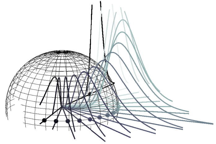
Certain kinds of data are not well-modeled under the assumption of an underlying Euclidean geometry. Examples include data with a fundamental directional structure, data that represents transformations of Euclidean space (such as rotations and reflections), data that has periodicity constraints or data that represents hierarchical structures. In such cases, it is important to explicitly model the data as lying on a manifold with a suitable structure; for instance a sphere would be appropriate for directional data, the orthogonal group for rotations and reflections, and the torus captures structural properties of periodicity.
The first contribution of this work is to express density estimation on manifolds as a form of dequantization. Given a probability density in an ambient Euclidean space, one can obtain the density on the manifold by performing a manifold change-of-variables in which the manifold structure appears and then projecting out any auxiliary structures. This marginalization can be viewed as analogous to “quantization” where, for instance, continuous values are discarded and only rounded integer values remain. In this view the auxiliary structure defines how the manifold could be “dequantized” into the ambient Euclidean space. By marginalizing the auxiliary dimensions, the marginal distribution on the manifold is obtained. In practice, however, one has only the manifold-constrained observations from an unknown distribution on the manifold. A second contribution of this work is to formulate the density estimation as a learning problem on the ambient Euclidean space. We show how to invoke the manifold change-of-variables and perform the marginalization along the auxiliary dimensions to obtain effective estimates of the density on the manifold. An advantage of our dequantization approach is that it allows one to utilize any expressive density directly on the ambient Euclidean space (e.g., RealNVP [Dinh et al. 2017], neural ODEs [Chen et al. 2018, Grathwohl et al. 2018] or any other normalizing flow [Kobyzev et al. 2020]); the dequantization approach does not require a practitioner to construct densities intrinsically on the manifold. We emphasize that our theory can be applied to any embedded manifold, provided one can identify a suitable auxiliary manifold structure and manifold change-of-variables to Euclidean space; finding a suitable auxiliary structure may be a challenge in some cases. We focus our attention on several important matrix manifolds which are common in practice and provide suitable structures for them.
2 Illustrative Example: Sphere
We first offer a simple example to illustrate how the method may be applied to obtain densities on the sphere. Let represent the 2-dimensional sphere viewed naturally as an embedded manifold of 3-dimensional Euclidean space. Excluding the point , observe that every other point may be uniquely identified with a point and positive real number such that . Thus, represents a spherical coordinate system for . If is a density on (equivalent to up to a set of Lebesgue measure zero), we can apply the standard change-of-variables formula in order to obtain a density on :
| (1) |
where is the associated Jacobian determinant accounting for changes in volume. We will refer to as the ambient Euclidean distribution.
By sampling with density , converting to the spherical coordinate system and discarding the radius , we obtain a sample from the marginal distribution on the sphere . The density is given by:
| (2) |
This density can be evaluated using importance sampling using a non-vanishing density on ,
| (3) |
We note that may depend on . A visualization of these concepts is presented in fig. 1.
Equation 2 quantizes to by integrating out the auxiliary dimension. Equation 3 describes how to marginalize over to compute the density of a quantized point ; hence, we refer to as the dequantization density. Taking the log of eq. 3, and invoking Jensen’s inequality we can also obtain the following lower bound on the marginal log-probability of :
| (4) |
Finally, we can use eq. 1 to express both eq. 3 and eq. 4 in terms of the density on the ambient Euclidean space .
Learning the Distributions: Sphere Example. In order to make these densities learnable, we introduce parameters and and write and . For instance, could be a normalizing flow parameterized by and could be a log-normal distribution whose mean and variance parameters are determined by a neural network with parameters and input .
We can use eq. 4 as an objective function for performing density estimation on the sphere. Given samples we compute a lower bound on the marginal log-probability as,
| (5) |
We can then maximize the right-hand side with respect to and . This yields a procedure for estimating the density on a sphere by transforming a density in an ambient Euclidean space and marginalizing over the radial dimension. The learned distribution on the ambient space is represented using a normalizing flow. This allows us to sample and to evaluate the density . Therefore, to sample from the learned we simply sample , and then project it to the sphere: .
Evaluating the Density: Sphere Example. Next, we may wish to evaluate the learned density . The normalizing flow provides us with the learned density in the ambient space, which immediately gives us the density through eq. 1, we must marginalize over so as to obtain a density on . We return to eq. 2 and use the dequantization distribution to evaluate using importance sampling.
3 Related Work
The general problem of density estimation is well studied and a full review is beyond the scope of this paper. The most directly related work is in the area of density estimation with normalizing flows and we refer readers to the review articles by [Papamakarios et al. 2019] and [Kobyzev et al. 2020].
From the perspective of estimating general densities on smooth manifolds, our work is related to [Rezende et al. 2020], which considers normalizing flows on tori and spheres. [Bose et al. 2020] defines a class of normalizing flows on hyperbolic spaces. [Wang and Gelfand 2013] considers the density of a multivariate normal random variable projected to the sphere via the mapping . For methods on connected Lie groups, one may use the exponential map in order to smoothly parameterize an element of the group by a coordinate in Euclidean space; this was the approach adopted in [Falorsi et al. 2019]. [Lou et al. 2020] extended continuous normalizing flows to manifolds by defining and simulating ordinary differential equations on the manifold. In contrast to these approaches, the method proposed here allows for the use of any density estimation technique defined on the ambient Euclidean space.
This work was inspired by dequantization techniques for normalizing flows. Originally introduced by [Uria et al. 2013] to account for the discrete nature of pixel intensities, the basic approach added (uniform) continuous noise to discrete values. This prevented the pathological behaviour that is known to occur when fitting continuous density models to discrete data [Theis et al. 2016]. The technique was extended by [Ho et al. 2019] to allow the added noise distribution to be learned using a variational objective which has become critical for strong quantitative performance in image modelling. [Hoogeboom et al. 2020] generalized the variational objective used for learning the dequantization noise distribution. Recently [Lippe and Gavves 2021] extended normalizing flows to categorical distributions. Our work proposes a new perspective on these approaches that the ambient Euclidean space (over which a continuous density model is learned) is a product of a discrete space (e.g., pixel intensities or discrete categories) and a continuous space which is projected (or “quantized”) when data is observed. Our work is a generalization of dequantization to consider not only discrete spaces, but also other structured spaces, specifically non-Euclidean manifolds.
4 Preliminaries
Let denote the identity matrix. If and are isomorphic sets we denote this by . The set of -valued, full-rank matrices () is denoted . The set of full-rank matrices is denoted , the generalized linear group. A matrix is positive definite if for all we have . The set of all positive definite matrices is denoted . When is a positive-definite matrix we denote the principal matrix square root by . We now consider several examples of embedded manifolds; see also appendix I for details on manifold embeddings. We focus our discussion around these examples because of their importance in data science applications.
Example 1 (Hypersphere).
The sphere in is defined by, . The sphere is an important manifold for data with a directional component (such as the line-of-sight of an optical receiver) or data that naturally lies on the surface of a spherical body (such as occurrences of solar flares on a star).
Example 2 (Torus).
The torus is the product manifold of circles . The torus can be embedded in by embedding each circle individually in . The torus is an important manifold for studying systems with several angular degrees of freedom (such as applications to robotic arms) or systems with periodic boundaries [Rezende et al. 2020].
Example 3 (Stiefel Manifold and Orthogonal Group).
The Stiefel manifold represents orthogonality constraints in a vector space. It may be regarded as the manifold of orthonormal vectors within a larger ambient Euclidean space. The Stiefel manifold can be leveraged for low-rank matrix completion. An important variant of the Stiefel manifold is the orthogonal group, which is the collection of all linear transformations of Euclidean space that preserve distance. The Stiefel manifold of order is defined by, . The -dimensional orthogonal group is defined by . Applications of the orthogonal group include the Procrustes problem, which describes the optimal rotation and reflection transformations that best align one cloud of particles toward another [Doucet et al. 2001]. The special orthogonal group is a subgroup of that satisfies the additional property that they have unit determinant. Formally, .
5 Theory
For our theoretical development, the most important tool is the change-of-variables formula for embedded manifolds; see inter alia [Rezende et al. 2020].
Theorem 1.
Let and be smooth manifolds embedded in and , respectively. Let be a smooth, invertible transformation. Let be a density on . Under the change-of-variables , the corresponding density on is given by,
| (6) |
where .
Even when is not an invertible mapping, it may be possible to compute the change-of-variables when is invertible on partitions of .
Corollary 1.
Let be a partition of . Let be a function and suppose that there exist smooth and invertible functions such that for . Then, if , the density of is given by where .
How does theorem 1 relate to the dequantization of smooth manifolds? Manifolds (such the sphere, the torus, or the orthogonal group) can be introduced as elements of a new coordinate system for an ambient Euclidean space. By marginalizing out the other dimensions of the new coordinate system, we obtain the distribution on the manifold of interest. We have already seen an example of this in section 2 where was transformed into a spherical coordinate system. We generalize this as follows:
Example 4 (Hypersphere).
The hyperspherical coordinate transformation giving the isomorphism of and is defined by, where . The inverse transformation is . The Jacobian determinant of the hyperspherical coordinate transformation is . Hence, given a density on (equivalent to up to a set of Lebesgue measure zero) we may compute the change-of-variables so as to obtain a density on by applying theorem 1 and the fact that the Jacobian determinant of the transformation is .
Example 5 (Torus).
From the fact that (a consequence of the polar coordinate transformation), we may similarly develop a coordinate system of even-dimensional Euclidean space in which the torus appears. Recall that (there are terms in the product). Therefore, we have established that . The isomorphism can be explicitly constructed by writing and defining the map by where . As the concatenation of polar coordinate transformations, the Jacobian determinant of this transformation is . The inverse transformation from back to is given by where . In the case of the torus, the product is the dequantization dimension of into . We describe a different means of dequantization, called modulus dequantization, in appendix C.
5.1 Stiefel Manifold
The coordinate transformation in which the Stiefel manifold appears requires a more involved construction than was the case for the sphere or torus. We first recall the relationship between the Stiefel manifold, full-rank matrices, and positive definite matrices: .The isomorphism of these spaces is constructed by the polar decomposition. Given , define, and . Thus, the isomorphism is given by . This isomorphism is rigorously established in appendix D.
Integrating over may be non-trivial due to the complicated structure of the positive-definite manifold of matrices. However, there is an isomorphism of and , the set of lower-triangular matrices with strictly positive entries on the diagonal. The isomorphism is given by the Cholesky decomposition: If then there is a unique matrix such that . We have therefore proved . One can use automatic differentiation in order to compute the Jacobian determinant of the transformation defined by . We call the transformation the Cholesky polar decomposition. The inverse transformation is
The Stiefel manifold is a generalization of the orthogonal group and we recover the latter exactly when . In this case, we identify as so that we obtain .
Finally we observe that almost all matrices are full-rank. Therefore, if one has a density in then we may apply the polar decomposition coordinate transformation in order to obtain a density on . Here plays the role of the dequantization dimension of into . An alternative coordinate transformation based on the QR decomposition instead of the polar decomposition is given in appendix J.
5.2 Dequantization
We have now seen how several manifolds appear in coordinate systems. In each case, the manifold appears with an auxiliary manifold which may not be of immediate interest. Namely, (i) The sphere appears with set of positive real numbers when defining a coordinate system for ; (ii) The torus appears the product manifold of copies of the positive real numbers when defining a coordinate system for ; (iii) the Stiefel manifold appears with the set of lower-triangular matrices with positive diagonal entries when defining a coordinate system of . We would like to marginalize out these “nuisance manifolds” so as to obtain distributions on the manifold of primary interest. A convenient means to achieve this is to introduce an importance sampling distribution over the nuisance manifold. Formally, we have the following result, which is an immediate consequence of theorem 1.
Corollary 2.
Let , , , and be as defined in theorem 1. Let be a non-vanishing density on . To obtain the marginal density on , let and it suffices to compute,
| (7) |
We consider some examples of marginalizing out the nuisance manifolds in some cases of interest.
Example 6 (Hypersphere).
Let be the hyperspherical coordinate transformation described in example 4. Given a density on , the manifold change-of-variables formula says that the corresponding density on is To obtain the marginal distribution we compute, . Or, using an importance sampling distribution whose support is , we obtain, .
Example 7 (Torus).
Example 8 (Stiefel Manifold).
Let be the Cholesky polar decomposition coordinate transformation described in section 5.1. Given a density in , we can construct the corresponding density on by applying theorem 1 as where and . To construct a importance sampling distribution over , one could generate the diagonal entries of and the remaining entries in the lower triangle according to . Applying corollary 2 gives the importance sampling formula for the marginal density on :
| (8) |
6 Discussion
| (9) |
We investigate the problem of density estimation given observations on a manifold using the dequantization procedure described in section 5. Let be a manifold embedded in and let be a density on . Given observations of , we wish to construct an estimate of the density . Algorithm 1 shows how we may apply dequantization for the purposes of density estimation provided that we have samples from the target density. We apply eq. 7 in order to obtain the density estimate on . Generating samples from may be achieved by first sampling , applying the transformation , and taking as a sample from the approximated distribution .
Densities on . As is a Euclidean space, we have available a wealth of possible mechanisms to produce flexible densities in the ambient space. One popular choice is RealNVP [Dinh et al. 2017]. In this case is the parameters of the underlying RealNVP network. An alternative is neural ODEs wherein parameterizes a vector field in the Euclidean space; the change in probability density under the vector field flow is obtained by integrating the instantaneous change-of-variables formula [Chen et al. 2018, Grathwohl et al. 2018].
Objective Functions. We consider two possible objective functions for density estimation. The first is the evidence lower bound of the observations :
| (10) |
This follows as a consequence of Jensen’s inequality applied to eq. 7. Experimental results using this objective function are denoted with the suffix (ELBO). The second is the log-likelihood computed via importance sampling:
| (11) |
Because the calculation of eq. 11 requires an importance sampling estimate, experimental results using this objective function are denoted with the suffix (I.S.).
7 Experimental Results
To demonstrate the effectiveness of the approach, we now show experimental results for density estimation on three different manifolds: the sphere, the torus and the orthogonal group. In our comparison against competing algorithms, we ensure that each method has a comparable number of learnable parameters. Our evaluation metrics are designed to test the fidelity of the density estimate to the target distribution; details on evaluation metrics are given in appendix G. In all of our examples we use rejection sampling in order to draw samples from the target distribution.


| Method | Mean MSE | Covariance MSE | Relative ESS | ||
|---|---|---|---|---|---|
| Deq. ODE (ELBO) | 0.0012 0.0002 | 0.0006 0.0001 | 0.0046 0.0002 | 0.0046 0.0002 | 99.0990 0.0401 |
| Deq. ODE (I.S.) | 0.0014 0.0002 | 0.0010 0.0001 | 0.0029 0.0001 | 0.0029 0.0001 | 99.4170 0.0225 |
| Deq RealNVP (ELBO) | 0.0004 0.0001 | 0.0003 0.0001 | 0.0231 0.0010 | 0.0212 0.0009 | 95.9540 0.1688 |
| Deq. RealNVP (I.S.) | 0.0005 0.0002 | 0.0002 0.0000 | 0.0124 0.0006 | 0.0115 0.0006 | 97.8240 0.1183 |
| Man. ODE | 0.0010 0.0004 | 0.0009 0.0002 | 0.0085 0.0007 | 0.0083 0.0007 | 98.3860 0.1328 |
| Möbius | 0.0021 0.0005 | 0.0019 0.0005 | 0.0595 0.0025 | — | 89.2575 0.4888 |
| Method | Mean MSE | Covariance MSE | Relative ESS | ||
|---|---|---|---|---|---|
| Deq. ODE (ELBO) | 0.0009 0.0001 | 0.0007 0.0001 | 0.0072 0.0002 | 0.0070 0.0002 | 98.6490 0.0388 |
| Deq. ODE (I.S.) | 0.0017 0.0001 | 0.0022 0.0002 | 0.0189 0.0004 | 0.0180 0.0004 | 96.6150 0.0648 |
| Deq. RealNVP (ELBO) | 0.0003 0.0001 | 0.0004 0.0001 | 0.0384 0.0010 | 0.0283 0.0005 | 95.1880 0.0771 |
| Deq. RealNVP (I.S.) | 0.0003 0.0001 | 0.0003 0.0000 | 0.0208 0.0004 | 0.0180 0.0004 | 96.6340 0.0920 |
| Man. ODE | 0.0012 0.0003 | 0.0008 0.0002 | 0.0098 0.0009 | 0.0094 0.0007 | 98.1780 0.1302 |
| Möbius | 0.0027 0.0004 | 0.0014 0.0003 | 0.0542 0.0047 | — | 88.7290 0.9332 |
Sphere and Hypersphere. Our first experimental results concern the sphere where we consider a multimodal distribution with four modes. This density on which is visualized in fig. 3. We consider performing density estimation using the ELBO (eq. 10) and log-likelihood objective functions (eq. 11); we construct densities in the ambient space using RealNVP and neural ODEs. We use algorithm 1 to learn the parameters of the ambient and dequantization distributions. As baselines we consider the Möbius transform approach described in [Rezende et al. 2020], which is a specialized normalizing flow method for tori and spheres, and the neural manifold ODE applied to the sphere as described in [Lou et al. 2020]. We give a comparison of performance metrics between these methods in table 1. In these experiments, we find that parameterizing a neural ODE model in the ambient space gave the better KL-divergence and effective sample size (ESS) metrics than RealNVP when our dequantization approach is used. We find that our dequantization algorithm minimizing either eq. 10 or eq. 11 achieves similar performance in the first and second moment metrics. However, when using eq. 11, slightly lower KL-divergence metrics are achievable as well as slightly larger effective sample sizes. In either case, dequantization outperforms the Möbius transform on this multimodal density on . The manifold ODE method is outperformed by the ODE dequantization algorithms with both eq. 10 and eq. 11.
| Density | Method | Mean MSE | Covariance MSE | Relative ESS | ||
|---|---|---|---|---|---|---|
| Correlated | Deq. RealNVP (ELBO) | 0.0019 0.0007 | 0.0098 0.0019 | 0.0072 0.0005 | 0.0084 0.0006 | 98.6510 0.0958 |
| Deq. RealNVP (I.S.) | 0.0024 0.0007 | 0.0121 0.0041 | 0.0038 0.0004 | 0.0040 0.0004 | 99.2570 0.0796 | |
| Modulus | 0.0017 0.0005 | 0.0072 0.0021 | 0.0025 0.0006 | 0.0025 0.0006 | 99.5000 0.1153 | |
| Möbius | 0.0004 0.0002 | 0.0083 0.0029 | 0.0021 0.0002 | — | 99.5850 0.0332 | |
| Unimodal | Deq. RealNVP (ELBO) | 0.0010 0.0003 | 0.0133 0.0040 | 0.0066 0.0004 | 0.0079 0.0004 | 98.7240 0.0761 |
| Deq. RealNVP (I.S.) | 0.0011 0.0003 | 0.0081 0.0020 | 0.0021 0.0002 | 0.0023 0.0002 | 99.5980 0.0317 | |
| Modulus | 0.0014 0.0003 | 0.0164 0.0028 | 0.0028 0.0003 | 0.0028 0.0003 | 99.4340 0.0531 | |
| Möbius | 0.0006 0.0002 | 0.0055 0.0037 | 0.0008 0.0001 | — | 99.8490 0.0293 | |
| Multimodal | Deq. RealNVP (ELBO) | 0.0024 0.0006 | 0.0158 0.0026 | 0.0065 0.0002 | 0.0075 0.0002 | 98.7800 0.0379 |
| Deq. RealNVP (I.S.) | 0.0007 0.0002 | 0.0061 0.0014 | 0.0020 0.0001 | 0.0022 0.0002 | 99.6160 0.0288 | |
| Modulus | 0.0016 0.0007 | 0.0063 0.0024 | 0.0035 0.0004 | 0.0035 0.0004 | 99.3030 0.0725 | |
| Möbius | 0.0006 0.0001 | 0.0070 0.0039 | 0.0012 0.0002 | — | 99.7600 0.0358 |
| Experiment | Mean MSE | Covariance MSE | Relative ESS | ||
|---|---|---|---|---|---|
| Procrustes (ELBO - Polar) | 0.0021 0.0008 | 0.0012 0.0005 | 0.0193 0.0069 | 0.0173 0.0053 | 96.9489 0.7649 |
| Procrustes (I.S. - Polar) | 0.0038 0.0020 | 0.0015 0.0008 | 0.0301 0.0126 | 0.0202 0.0075 | 95.6944 1.4654 |
| Procrustes (ELBO - QR) | 0.0011 0.0003 | 0.0008 0.0003 | 0.0124 0.0032 | 0.0095 0.0015 | 97.9678 0.3325 |
| Procrustes (I.S. - QR) | 0.0015 0.0005 | 0.0011 0.0004 | 0.0174 0.0072 | 0.0122 0.0029 | 96.6267 0.6326 |
| (ELBO - Polar) | 0.0007 0.0002 | 0.0029 0.0003 | 0.0443 0.0011 | 0.0415 0.0059 | 96.2930 0.0649 |
| (I.S. - Polar) | 0.0004 0.0001 | 0.0014 0.0001 | 0.0207 0.0028 | 0.0235 0.0029 | 97.7280 0.1136 |
| (ELBO - QR) | 0.0017 0.0004 | 0.0054 0.0006 | 0.0563 0.0060 | 0.0363 0.0041 | 93.5633 2.1331 |
| (I.S. - QR) | 0.0012 0.0004 | 0.0020 0.0004 | 0.0260 0.0017 | 0.0219 0.0021 | 94.3256 2.8099 |
We next consider a multimodal density (the special unitary group). As before, we compare dequantization to Möbius flow transformations and manifold neural ODEs and present results in table 2. Similar to the case of the multimodal density on , we find that dequantization with an ambient neural ODE model is most effective, with ELBO maximization giving the smallest KL-divergence metrics. All dequantization algorithms out-performed the Möbius transformation on the sphere but only dequantization with an ambient ODE and ELBO minimization outperformed the manifold neural ODE method.
Torus. We next consider three densities from [Rezende et al. 2020] on the torus . These densities are, respectively, unimodal, multimodal, or exhibit strongly correlated dimensions. As in the case of the sphere, we evaluate dequantization of the torus against the Möbius transform method. As a further point of comparison, we also consider learning a normalizing flow density on and simply identifying every -periodic point so as to induce distribution on ; we call this the modulus dequantization method. Results are reported in table 3. We find that the Möbius transformation performs strongest in this comparison. The modulus method also performs well, particularly on the correlated toroidal density function. Of the dequantization-based approaches, minimizing the negative log-likelihood produces the best performance, which outperforms the modulus method in terms of KL-divergence and first- and second-moment metrics (excepting the correlated density). We note, however, that all of these methods estimated effective sample sizes at nearly 100%, indicating that the differences between each approach, while statistically significant, are practically marginal.
Orthogonal Group. The previous two examples focused on manifolds composed of spheres and circles. We now examine density estimation on the orthogonal group, where we consider inference in a probabilistic variant of the orthogonal Procrustes problem; we seek to sample orthogonal transformations that transport one point cloud towards another in terms of squared distance. We consider parameterizing a distribution in the ambient Euclidean space using RealNVP in these experiments. Results are presented in table 4. We observe that optimizing the ELBO objective function (eq. 10) tended to produce better density estimates than the log-likelihood (eq. 11). Nevertheless, we find that either dequantization algorithm is effective at matching the target density.
We may also leverage corollary 1 so as to apply our method to the “dequantization” of . As an example, we consider a multimodal density on . Results of applying our method to sampling from this distribution are also shown in table 4. In this example we find that minimizing the negative log-likelihood using importance sampling tended to produce the best approximation of the first- and second-moments of the distribution, in addition to smaller KL-divergence metrics.
8 Conclusion
This paper proposed a new method for density estimation on manifolds called manifold dequantization. The proposed approach allows us to make use of existing techniques for density estimation on Euclidean spaces while still providing efficient, exact sampling of the distribution on the manifold as well as approximate density calculation. We evaluated this method for densities on the sphere, the torus, and the orthogonal group. Our results show that manifold dequantization is competitive with, or exceeds the performance of, competing methods for density estimation on manifolds.
In terms of societal impact, matrix manifolds appear in various scientific disciples such as computational biology, the earth sciences, and robotics. While our experimentation on dequantization are synthetic, techniques proposed here could be adapted to research in these scientific disciplines in unforeseen ways.
References
- Bogachev et al. [2007] V. Bogachev, A. Kolesnikov, and K. Medvedev. Triangular transformations of measures. Sbornik: Mathematics, 196:309, 10 2007. doi: 10.1070/SM2005v196n03ABEH000882.
- Bose et al. [2020] J. Bose, A. Smofsky, R. Liao, P. Panangaden, and W. Hamilton. Latent variable modelling with hyperbolic normalizing flows. In H. D. III and A. Singh, editors, Proceedings of the 37th International Conference on Machine Learning, volume 119 of Proceedings of Machine Learning Research, pages 1045–1055. PMLR, 13–18 Jul 2020. URL http://proceedings.mlr.press/v119/bose20a.html.
- Chen et al. [2018] R. T. Q. Chen, Y. Rubanova, J. Bettencourt, and D. K. Duvenaud. Neural ordinary differential equations. In S. Bengio, H. Wallach, H. Larochelle, K. Grauman, N. Cesa-Bianchi, and R. Garnett, editors, Advances in Neural Information Processing Systems, volume 31, pages 6571–6583. Curran Associates, Inc., 2018. URL https://proceedings.neurips.cc/paper/2018/file/69386f6bb1dfed68692a24c8686939b9-Paper.pdf.
- Dinh et al. [2017] L. Dinh, J. Sohl-Dickstein, and S. Bengio. Density estimation using real NVP. In 5th International Conference on Learning Representations, ICLR 2017, Toulon, France, April 24-26, 2017, Conference Track Proceedings. OpenReview.net, 2017. URL https://openreview.net/forum?id=HkpbnH9lx.
- Doucet et al. [2001] A. Doucet, A. Smith, N. de Freitas, and N. Gordon. Sequential Monte Carlo Methods in Practice. Information Science and Statistics. Springer New York, 2001. ISBN 9780387951461. URL https://books.google.com/books?id=uxX-koqKtMMC.
- Edelman [1989] A. Edelman. Eigenvalues and Condition Numbers of Random Matrices. Massachusetts Institute of Technology, 1989.
- Falorsi et al. [2019] L. Falorsi, P. de Haan, T. R. Davidson, and P. Forré. Reparameterizing distributions on lie groups. Proceedings of Machine Learning Research, 89:3244–3253, 16–18 Apr 2019. URL http://proceedings.mlr.press/v89/falorsi19a.html.
- Federer [1969] H. Federer. Geometric Measure Theory. Die Grundlehren der mathematischen Wissenschaften in Einzeldarstellungen. Springer, 1969. ISBN 9780387045054. URL https://books.google.com/books?id=TALvAAAAMAAJ.
- Gower and Dijksterhuis [2004] J. C. Gower and G. B. Dijksterhuis. Procrustes Problems. Oxford University Press, 2004. ISBN 9780198510581.
- Grathwohl et al. [2018] W. Grathwohl, R. T. Q. Chen, J. Bettencourt, I. Sutskever, and D. Duvenaud. Ffjord: Free-form continuous dynamics for scalable reversible generative models, 2018.
- Ho et al. [2019] J. Ho, X. Chen, A. Srinivas, Y. Duan, and P. Abbeel. Flow++: Improving flow-based generative models with variational dequantization and architecture design, 2019.
- Hoogeboom et al. [2020] E. Hoogeboom, T. S. Cohen, and J. M. Tomczak. Learning discrete distributions by dequantization, 2020.
- Huang et al. [2018] C.-W. Huang, D. Krueger, A. Lacoste, and A. Courville. Neural autoregressive flows. In J. Dy and A. Krause, editors, Proceedings of the 35th International Conference on Machine Learning, volume 80 of Proceedings of Machine Learning Research, pages 2078–2087. PMLR, 10–15 Jul 2018. URL http://proceedings.mlr.press/v80/huang18d.html.
- Jaini et al. [2019] P. Jaini, K. A. Selby, and Y. Yu. Sum-of-squares polynomial flow. In K. Chaudhuri and R. Salakhutdinov, editors, Proceedings of the 36th International Conference on Machine Learning, volume 97 of Proceedings of Machine Learning Research, pages 3009–3018. PMLR, 09–15 Jun 2019. URL http://proceedings.mlr.press/v97/jaini19a.html.
- Jones [2004] F. Jones. Integration on manifolds, 2004. URL http://www.owlnet.rice.edu/%7Efjones/chap11.pdf.
- Kobyzev et al. [2020] I. Kobyzev, S. Prince, and M. Brubaker. Normalizing flows: An introduction and review of current methods. IEEE Transactions on Pattern Analysis and Machine Intelligence, 2020.
- Lee [2003] J. Lee. Introduction to Smooth Manifolds. Graduate Texts in Mathematics. Springer, 2003. ISBN 9780387954486. URL https://books.google.com/books?id=eqfgZtjQceYC.
- Lippe and Gavves [2021] P. Lippe and E. Gavves. Categorical normalizing flows via continuous transformations, 2021.
- Liu [2008] J. S. Liu. Monte Carlo Strategies in Scientific Computing. Springer Publishing Company, Incorporated, 2008. ISBN 0387763694.
- Lou et al. [2020] A. Lou, D. Lim, I. Katsman, L. Huang, Q. Jiang, S.-N. Lim, and C. De Sa. Neural manifold ordinary differential equations. arXiv preprint arXiv:2006.10254, 2020.
- Papamakarios et al. [2019] G. Papamakarios, E. Nalisnick, D. J. Rezende, S. Mohamed, and B. Lakshminarayanan. Normalizing flows for probabilistic modeling and inference, 2019.
- Rezende et al. [2020] D. J. Rezende, G. Papamakarios, S. Racanière, M. S. Albergo, G. Kanwar, P. E. Shanahan, and K. Cranmer. Normalizing flows on tori and spheres. CoRR, abs/2002.02428, 2020. URL https://arxiv.org/abs/2002.02428.
- Theis et al. [2016] L. Theis, A. van den Oord, and M. Bethge. A note on the evaluation of generative models, 2016.
- Uria et al. [2013] B. Uria, I. Murray, and H. Larochelle. Rnade: The real-valued neural autoregressive density-estimator. arXiv preprint arXiv:1306.0186, 2013.
- Villani [2008] C. Villani. Optimal Transport: Old and New. Grundlehren der mathematischen Wissenschaften. Springer Berlin Heidelberg, 2008. ISBN 9783540710509. URL https://books.google.com/books?id=hV8o5R7_5tkC.
- Wang and Gelfand [2013] F. Wang and A. E. Gelfand. Directional data analysis under the general projected normal distribution. Statistical Methodology, 10(1):113 – 127, 2013. ISSN 1572-3127. doi: https://doi.org/10.1016/j.stamet.2012.07.005. URL http://www.sciencedirect.com/science/article/pii/S1572312712000457.
Appendix A Evidence Lower Bound for Special Orthogonal Group
Let be a reflection matrix. Then using the fact that we have,
| (12) | ||||
| (13) | ||||
| (14) | ||||
| (15) |
where .
Appendix B Dequantizing the Integers
We now consider how to apply corollaries 1 and 1 to the dequantization of integers and draw a connection to dequantization in normalizing flows [Hoogeboom et al. 2020]. Let be a probability density on . Consider the function defined by . Consider the partition of given by ; on each we have that satisfies ; moreover, on each , the transformation is invertible (the inverse map is ) and preserves volume, which implies a unit Jacobian determinant. Therefore, the associated density on is given by . We may view as a coordinate system for . If we wish to integrate out the nuisance variables in the unit interval, we obtain the marginal density on as
| (16) |
By choosing as, for example, a Uniform distribution, one obtains the traditional uniform dequantization. Choosing a more complex distribution, for example, a Beta distribution (with parameters possibly depending on ) one obtains an importance sampling formula for the marginal density as . This can be optimized through a variational bound, giving variational dequantization [Ho et al. 2019]. Optimizing it directing gives importance weighted dequantization [Hoogeboom et al. 2020].
Appendix C Torus Modulus Dequantization
Taking inspiration from appendix B, we turn now to consider another dequantization of the torus. To begin, identify the circle with the interval . We can construct a map from to by identifying -periodic points. Define the map . Let for ; on this interval we may define by which satisfies . Because this map is nothing but a shift by , it is invertible and volume preserving. Moreover, we may view as a coordinate system for . Let be a density on and let . The associated density on is therefore,
| (17) |
We may marginalize out the integers to obtain the density on as
| (18) |
This idea is readily extended to higher dimensions. Because the torus is nothing but the product manifold of two circles, we may identify the torus with . Let be a density on and let be defined by . Following the precise reasoning from the one-dimensional case, if then the density of is,
| (19) |
We call this approach modulus dequantization. This approach requires fewer dimensions than embedding the torus in . In practice, the infinite sums over the integers may be approximated by truncating to a finite number of terms.
Appendix D Polar Decomposition Isomorphism
Proposition 1.
Let be a real, positive semi-definite matrix. Then there exists a unique real, positive semi-definite matrix such that . We call the principal square root of and may write .
Definition 1 (Stiefel Manifold).
The manifold is the subset of of orthogonal matrices. That is,
| (20) |
Definition 2.
The set of positive-definite matrices is denoted .
Definition 3 (Non-Square Polar Decomposition).
Let with have the (thin) singular value decomposition where and . Then we define the non-square polar decomposition to be where,
| (21) | ||||
| (22) |
Lemma 1.
The quantity in eq. 22 is uniquely defined.
Proof.
The strategy is to show that is the unique principal square root of a positive semi-definite matrix. It is immediately clear from the definition that is itself positive semi-definite. Consider the positive semi-definite matrix
| (23) | ||||
| (24) | ||||
| (25) | ||||
| (26) |
By identification is the principal square root of so it is unique. ∎
Proposition 2.
Let and suppose that . Then, the quantity in eq. 21 is uniquely defined.
Proof.
If then
| (27) | ||||
| (28) | ||||
| (29) |
Thus, is invertible. Thus, . ∎
Note that the condition on the singular values is equivalent to the statement that has full-rank.
Lemma 2.
If has full-rank then .
Proof.
If has full-rank then all the singular values are strictly positive. Thus, is an eigen-decomposition of whose eigenvalues are all positive. Since a matrix is positive-definite if and only if all of its eigenvalues are positive, we conclude that . ∎
Lemma 3.
The quantity in eq. 21 is an element of .
Proof.
| (30) | ||||
| (31) | ||||
| (32) |
∎
Proof.
Since , by the spectral theorem there exists an orthonormal basis of and real, positive eigenvalues , such that where is the collection of as columns and .
Using this we may compute , which is an orthogonal matrix:
| (33) | ||||
| (34) | ||||
| (35) |
Define the matrix . By inspection, a (thin) singular value decomposition of is
| (36) |
since
| (37) | ||||
| (38) |
Finally, , has only positive entries, and , which are the conditions of a thin singular value decomposition. ∎
Appendix E Experimental Details
Here we include additional information about our experimental design.
E.1 Sphere
We consider the following unnormalized density on given by
| (39) |
where , , , and .
When using RealNVP, the total number of learnable parameters in our dequantization model is ; dequantization with an ambient ODE has learnable parameters; in the case of the Möbius transform the total number of learnable parameters is ; for the manifold ODE implementation, we have parameters.
On , we consider an unnormalized density proportional to
| (40) | ||||
| (41) | ||||
| (42) | ||||
| (43) | ||||
| (44) |
When using RealNVP, the total number of learnable parameters in our dequantization model is ; dequantization with an ambient ODE has learnable parameters; in the case of the Möbius transform the total number of learnable parameters is ; for the manifold ODE implementation, we have parameters. For dequantization we use 100 samples per batch and use rejection sampling to draw samples from the unnormalized target density at each iteration.
E.2 Torus
Expressed in terms of their angular coordinates (as opposed to their embedding into ), the densities on the torus are as follows:
- Unimodal
-
with .
- Multimodal
-
where , , and .
- Correlated
-
.
The number of learnable parameters in the dequantization models is ; in the Möbius flow model, the number of learnable parameters is ; for the direct method, the number of learnable parameters is . For dequantization we use 100 samples per batch and use rejection sampling to draw samples from the unnormalized target density at each iteration.
E.3 Orthogonal Group
Drawing inspiration from the orthogonal Procrustes problem, we define the unnormalized density by
| (45) |
where . Given samples from eq. 45, we may apply our dequantization procedure to perform density estimation. In our experiments we take and . For dequantization we use rejection sampling to draw samples from the posterior. Then, with these fixed samples, we use batches of 100 samples to train the ambient and dequantization distributions.
E.4 Special Orthogonal Group
Let be a reflection matrix and notice that is partition of . Given a density on , using the methods described in section 5.1, we may obtain a density on . Then, we define the function by
| (46) |
where is a reflection matrix. Now, define and , which satisfy and . Both and are self-inverse and volume-preserving maps on their respective domains so we may obtain a density on as
| (47) |
One may immediately seek to minimize the negative log-likelihood of data using eq. 47. Alternatively, we use the following ELBO in our our experiments:
| (48) |
where, as in example 8, . For a short derivation of this ELBO, see appendix A.
We consider the following multimodal density on :
| (49) |
where in our experiments we set , , , and . For dequantization we use rejection sampling to draw samples from the posterior. Then, with these fixed samples, we use batches of 100 samples to train the ambient and dequantization distributions.
Appendix F Practical Considerations
| Element | Notation | Description | |||
|---|---|---|---|---|---|
| Ambient Euclidean Space | Euclidean space in which the manifold of interest is embedded | ||||
| Ambient Density | A flexible family of densities parameterized by on | ||||
| Change-of-Variables Mapping |
| ||||
| Dequantization Density |
| ||||
| Loss Function |
|
F.1 The Ambient Euclidean Space
It is frequently the case that a manifold has a natural embedding into Euclidean space. For instance, the sphere is naturally embedded into . The Stiefel manifold is a subset of satisfying an orthonormality condition; therefore, it is naturally embedded into . For some manifolds, the choice may require some consideration. For instance, a torus may be regarded as a product manifold of two circles, each of which are naturally embedded into so that the entire torus is embedded into (this is called the Clifford torus). An alternative is the familiar embedding of the torus as a “doughnut” in , although in this case it may be non-obvious how to construct a suitable mapping between , the doughnut torus, and some auxiliary choice of one-dimensional manifold.
F.2 The Change-of-Variables and Auxiliary Manifold
We have seen several examples wherein manifolds of interest appear alongside an auxiliary manifold when an ambient Euclidean space is transformed under a change-of-variables. In general, one would like to identify a transformation , satisfying the conditions of theorem 1 or corollary 1, such that it will be straightforward to formulate importance sampling random variables on so as to obtain the marginal density on .
F.3 Dequantization Density
Dequantization densities on has to respect the constraints of the auxiliary manifold. For instance, if we must choose a dequantization density whose support is the positive real numbers and which is non-vanishing. The requirement that be non-vanishing (that is, for all ) is important so as to avoid division-by-zero singularities in the importance sampling formula eq. 7. We have already seen some examples of dequantization densities that respect the constraints of the auxiliary manifold in section 5. In each of these cases, the dequantization distribution is parameterized (for example, the Gamma distribution is parameterized by its shape and scale); it may be desirable to choose these parameters to depend on the location . To accomplish this, one may construct a neural network with parameters and input whose output is the parameterization of the dequantization distribution. Thus the dequantization distribution may be in general expressed as .
Appendix G Evaluation Metrics
Given a density , known up to proportionality, we consider several performance metrics for the dequantization method we propose. The error of the first order moment is defined by,
| (50) |
The error of the second (centered) moment is defined by
| (51) |
The Kullback-Leibler divergence of and is
| (52) | ||||
| (53) |
where is the normalizing constant of . We can estimate via importance sampling according to
| (54) |
which permits us to compute a Monte Carlo estimate of the Kullback-Leibler divergence. The reverse direction of the KL-divergence may be similarly computed.
Let be a collection of independent identically-distributed samples from . The number of effective independent samples is the quantity,
| (55) |
where . See [Liu 2008, Gower and Dijksterhuis 2004] for details on the ESS metric. Following [Rezende et al. 2020], we report the relative ESS, which the ratio of the effective sample size and , the number of samples. When a Monte Carlo approximation of the evaluation metric is required, we use rejection sampling in order to obtain samples from the density .
Appendix H Proof of Manifold Change-of-Variables Formula
Proposition 4.
Let and let be a smooth function. Suppose . Define the embedded manifold . Let be a real-valued, continuous function on . Then,
| (56) |
where is the volume measure on .
Proof.
See [Jones 2004]. ∎
Corollary 3.
Define,
| (57) |
Then rearranging immediately implies,
| (58) |
which is the manifold change-of-variables formula.
What follows now is a more detailed exposition on this result using Riemannian geometry.
Let be an open subset of . Let be a continuous function from that is a homeomorphism on its image. That is, defining , we find that has a continuous inverse on . As a subset of , we can equip with the subspace topology and find that is a topological -manifold. Under these assumptions, it immediately follows that is a global coordinate chart in the sense of differential geometry.
If we further assume that and its inverse are smooth functions (in the sense of ordinary calculus), then it follows that is globally diffeomorphic to . Evidently, our discussion allows . If the Jacobian (in the sense of ordinary calculus) of , denoted , has the property that at every , , then is called a smooth immersion; this is equivalent to having full-rank at each . Moreover, because is homeomorphic onto its image, is also a smooth embedding.
The tangent space of a smooth manifold can be constructed as the vector space of velocities that a particle moving along the manifold may exhibit at a point. Formally, let be an open interval and let be a parameterized smooth curve in . The composition is then a parameterized smooth curve on . The velocity of is then computed as,
| (59) |
From the preceding discussion, is a matrix of full-rank and therefore has linearly-independent -dimensional columns. Since can be arbitrary, we find that the tangent space of at is the vector space spanned by the columns of ; note that these basis vectors depend only on the position in and not on time. Given , we denote the tangent space by which is a vector subspace of . In the following, we make use of the common identification .
A smooth manifold can be turned into a Riemannian manifold by equipping its tangent spaces with an inner product called the Riemannian metric. Formally, given , where is an inner product. Given the discussion so far, there is no prescription for a Riemannian metric. However, we may “prefer” the Riemannian metric that is induced from the ambient Euclidean space . For , the Euclidean metric is defined by where . The induced metric on is then defined by where and are viewed as vectors in satisfying .
Given a metric on , we can compute an associated metric on called the pullback metric. The pullback metric is defined by,
| (60) | ||||
| (61) |
where . From the condition that is a matrix of full-rank for each , it can be shown that is a positive definite matrix. Hence the pullback metric is a proper inner product. Unlike the induced metric on which has no real dependency on , the pullback metric does depend on through . The pullback metric can be regarded as the expression of the induced metric on in the global coordinates of . Indeed, if , recall that every can be expressed as where ; the unique can be computed from
| (62) |
In our construction, we have described how to induce a metric on via the Euclidean metric in the embedding space. We then described how the metric materializes in the global coordinate system via the pullback metric. We are now in a position to state how these objects inform integration on Riemannian manifolds. We have the following theorem.
Theorem 2.
Let denote the Riemannian volume element on when the metric on is the induced Euclidean metric from . Given a smooth function , its integral over can be expressed in terms of the global coordinate system as,
| (63) |
A proof of this result may be found in [Jones 2004]. More sophisticated variants of this result may be found textbooks on differential geometry; see, inter alia, [Lee 2003].
If is a density on , and , then we have,
| (64) | ||||
| (65) | ||||
| (66) |
where
| (67) |
which, upon rearrangement, is the manifold change-of-variables formula.
Given a subset , we define its volume by,
| (68) |
Such a definition of volume is sometimes called the “surface measure” and it is a generalization of arclength in the one-dimensional setting. Moreover, this notion of volume coincides with the -dimensional Hausdorff area of ; this is a consequence of the area formula and a detailed discussion can be found in [Federer 1969].
Appendix I Embedded Manifolds
A smooth manifold of dimension is a second-countable Hausdorff space such that for every there is a homeomorphism between a neighborhood of and . By the Whitney Embedding Theorem (see, inter alia, [Lee 2003]), every smooth manifold can be smoothly embedded into Euclidean space of dimension . It is frequently possible to express an embedded manifold as the zero level-set of a constraint function: Let be a smooth function and define . If is a matrix of full-rank for every , we say that is an embedded manifold of rank . To see how these definitions apply, let us consider some examples.
I.1 Hypersphere
The sphere in is the zero level-set of the constraint function .
I.2 Torus
The torus is the preimage of the constraint function defined by
| (69) |
I.3 Stiefel Manifold
A constraint function for the manifold is defined by . Using the isomorphism, may also be embedded into .
Appendix J Stiefel QR Decomposition
In appendix D we discussed computing the positive definite component as the principal square root of . In our algorithm, is represented according to its Cholesky factor, which is unique because is (assuming is full-rank). An alternative would be to compute a Cholesky factor of directly; such an approach allows us to use the QR decomposition in place of the polar decomposition.
Proposition 5.
Suppose is a matrix of full-rank. The (unique) QR decomposition of is
| (70) |
where
| (71) | ||||
| (72) | ||||
| (73) |
Moreover .
Proof.
The uniqueness of (and consequently ) follows from the fact that the Cholesky decomposition of positive definite matrices is unique. Since is of full-rank, is a positive definite matrix. Since has positive diagonal entries, its determinant is non-zero and therefore has a unique inverse. This implies the uniqueness of . The fact that is an element of the Stiefel manifold follows from direct evaluation:
| (74) | ||||
| (75) | ||||
| (76) |
∎
Proposition 6.
Let . The Jacobian determinant of the transformation is
| (77) |
Proof.
See page 31 of [Edelman 1989]. ∎
Appendix K Overview of Normalizing Flows
This section describes the Euclidean normalizing flows used in this paper.
K.1 RealNVP
Let and let satisfy . Consider partitioning into components and by taking the first and last components from , respectively. Let and be a functions parameterized by and , respectively. Compute the affine transformation of according to
| (78) | |||
| (79) |
The transformation has a Jacobian of the form,
| (80) |
The key observation about this Jacobian is that it has a lower-triangular structure. Therefore, its determinant is the product of its diagonal elements.
The transformation is also invertible. Let be the corresponding partition of . The inverse map is given by,
| (81) | |||
| (82) |
With the inverse and Jacobian determinant available, we may apply the transformation in the Euclidean change-of-variables formula. This transformation is called RealNVP. In practice, it is common to chain multiple RealNVP transformations together in order to obtain a more expressive flow. One may also permute the elements of after each application of the RealNVP transformation (which is, of course, an invertible, volume-preserving transformation) in order to construct affine transformations of different variables.
K.2 Neural ODE
Let and let be a smooth function parameterized by . Consider solving the initial value problem defined by,
| (83) | ||||
| (84) |
The map is called the flow of . The existence and uniqueness of differential equations leads to the group property of flows:
| (85) |
In particular, since , we have or so that the inverse flow map is obtained from the flow map with a negated time index.
How does the flow of a vector field affect probability? This is an important question that can be answered at varying levels of sophistication. One elegant analysis uses techniques from fluid mechanics and the Lie derivative theorem. In the following we adopt a simpler, if more mechanical, derivation of the rate of change of the Jacobian determinant.
| (86) | ||||
| (87) | ||||
| (88) | ||||
| (89) | ||||
| (90) |
From which it follows that,
| (91) |
Let be a probability density and let . Let be the density of . Because , we have,
| (92) |
This formula is sometimes called the instantaneous change-of-variables formula. From the initial condition , we obtain that , which gives an initial condition for the time evolution of the Jacobian determinant.
In general, none of the initial value problems described so far have analytical solutions. This necessitates the use of numerical integrators to compute the map , its inverse, and the Jacobian determinant correction from the instantaneous change-of-variables formula. The method is called neural ODE because is often chosen to be a neural network parameterized by .
Appendix L Universal Approximation for the Dequantized Density
The purpose of this section is to give sufficient conditions on the dequantization of a distribution on a manifold into an ambient Euclidean space such that a suitably expressive normalizing flow on the Euclidean space could, in principle, learn the density to an arbitrary precision. The conclusion of this section is that it is sufficient that the distribution on the manifold and auxiliary structure be measurable with respect to the natural Borel -algebra and that the transformation between Euclidean space and the product space of the manifold and auxiliary structure be continuously differentiable. After stating this result, the remainder of the section is devoted to explaining what is meant by universal approximation of Euclidean densities.
Definition 4.
Let be a topological space. The smallest -algebra containing all the open sets of is called the Borel -algebra. The Borel -algebra is denoted . An element is called a Borel set.
Definition 5.
A measure on is said to be absolutely continuous with respect to the Lebesgue measure if there exists a measurable function such that
| (93) |
where .
Definition 6.
Let and be topological spaces. A function is said to be Borel measurable if for all
| (94) |
Proposition 7.
Let and be two Borel measurable functions. Then the product function is also Borel measurable. Moreover, if is another Borel measurable function then the composition is also Borel measurable.
Proposition 8.
Let be an open subset of and let be a homeomorphism on its image. Let . Assume further that is a continuously differentiable function. Let be a measure on that is absolutely continuous with respect to the volume measure on ; that is,
| (95) |
where is a measurable function and is a Borel subset. Then, if , the random variable has a measurable density with respect the the Lebesgue measure given by
| (96) |
Proof.
By the manifold change-of-variables formula, the measure is related to the Lebesgue measure on according to,
| (97) |
Now we apply the results of proposition 7 to show that the integrand on the right-hand side of eq. 97 is a measurable function. Because is smooth it is continuous, and continuous functions are measurable. Therefore, when we obtain that . Moreover, is a measurable function with respect to the Borel -algebra on because the composition of measurable functions is measurable. Finally, since is continuously differentiable, and since the determinant and square-root are continuous functions, is also a measurable function.
Thus, if , the random variable has a measurable density with respect the the Lebesgue measure given by
| (98) |
∎
Corollary 4.
The measure
| (99) |
is absolutely continuous with respect to the Lebesgue measure.
In the context of dequantization, we would like to understand the conditions under which the dequantization of a density on an embedded manifold via an auxiliary embedded manifold and a smooth, invertible function produces a Lebesgue measurable density on .
Proposition 9.
Let and be embedded manifolds. Let be the density on defined with respect to the Riemannian volume element and let be a density on (which may depend on ) defined with respect to the Riemannian volume element . Suppose further that , where is an open set of and is continuously differentiable homeomorphism. If are random variables having density function with respect to the product element , then the random variable has a density with respect to Lebesgue measure if is measurable with respect to .
Proof.
This follows as a result of proposition 8 when and is defined by
| (100) |
where . The conditions of the proposition are met because is an open subset of by assumption and is a continuously differentiable homeomorphism by assumption. ∎
The importance of the open set is best seen through an example.
Example 9.
Let and consider the transformation by defined by
| (101) |
where . Thus, we see that is the spherical coordinate representation of the point . The inverse of is given by . Notice that by choosing to exclude the zero vector, we ensure that is indeed a homeomorphism; if the zero vector had not been included we would find that for all so that the inverse is not unique.
To see that is continuously differentiable, we compute
| (102) | ||||
| (103) |
both of which are continuous for . Therefore, if is a random variable on with Borel-measurable density, then the random variable has a density in with respect to Lebesgue measure by proposition 9.
The existence of a Lebesgue measurable density in Euclidean space allows us to apply the theory of universal approximations of certain normalizing flows to guarantee that the dequantized distribution can be approximated arbitrarily well by a sufficiently expressive normalizing flow in Euclidean space.
The remaining discussion in this appendix is paraphrased from Section 3.4.3 in [Kobyzev et al. 2020], which itself draws from [Jaini et al. 2019] and [Huang et al. 2018]. The essential idea is that one can produce auto-regressive normalizing flows whose couplings are dense in a space of functions that are guaranteed to have a universality property.
Definition 7.
Let be a function and write where . Such a function is called triangular if depends only on
Definition 8.
Let be a function and write where . Such a function is called increasing if is an increasing function of .
Definition 9.
An auto-regressive normalizing flow is a triangular map of the form
| (104) |
where is a bijection parameterized by and is a map that parameterizes according to .
In our experimentation on dequantization, we have not considered using auto-regressive flows in the ambient Euclidean space; neither RealNVP nor neural ODEs are auto-regressive in the sense of definition 9. Therefore, this discussion is primarily of theoretical interest.
Definition 10.
Let be a probability measure on a measurable space and let be a random variable taking values in . We say that the law of is if for all Borel sets we have
| (105) |
The following result is from [Bogachev et al. 2007].
Proposition 10.
Let and be probability measures that are absolutely continuous with respect to the Lebesgue measure. Let be a random variable whose law is . Then there exists a triangular-increasing function such that the law of is .
A construction of such a map in proposition 10 is given by the Knothe-Rosenblatt rearrangement [Villani 2008].
The following result is from [Huang et al. 2018].
Lemma 4.
Let be a probability measure that is absolutely continuous with respect to Lebesgue measure. Let be a sequence of measurable maps converging pointwise to a map . If the law of a random variable is , then the random variables converge in law to to the random variable .
The universality of auto-regressive normalizing flows can therefore be established by demonstrating that the functions appearing in definition 9 are dense in the set of increasing monotone functions. One then applies propositions 10 and 4 to demonstrate that any random variable with law can be transformed by an auto-regressive flow using the function into an approximation of a random variable with law ; the approximation has arbitrarily high fidelity as measured by convergence in law. See [Huang et al. 2018, Jaini et al. 2019] for a discussion of parameterized families of functions that are known to possess this property.
In conclusion, proposition 9 gives the necessary conditions on product manifold densities and the change-of-variables to ensure the existence of a Lebesgue measurable density in an open subset of Euclidean space. We saw in example 9 how the choice of open set allows us to avoid pathological points in Euclidean space. Using the existence of the Lebesgue-measurable density, we may apply the theory of universal approximation of Lebesgue-measurable densities using auto-regressive normalizing flows to guarantee that the dequantized distribution can be approximated arbitrarily well. We note, however, that our experiments have not used auto-regressive normalizing flows.