ThetA - fast and robust clustering via a distance parameter
Abstract
Clustering is a fundamental problem in machine learning where distance-based approaches have dominated the field for many decades. This set of problems is often tackled by partitioning the data into K clusters where the number of clusters is chosen apriori. While significant progress has been made on these lines over the years, it is well established that as the number of clusters or dimensions increase, current approaches dwell in local minima resulting in suboptimal solutions. In this work, we propose a new set of distance threshold methods called Theta-based Algorithms (ThetA). Via experimental comparisons and complexity analyses we show that our proposed approach outperforms existing approaches in: a) clustering accuracy and b) time complexity. Additionally, we show that for a large class of problems, learning the optimal threshold is straightforward in comparison to learning K. Moreover, we show how ThetA can infer the sparsity of datasets in higher dimensions.
Keywords:
Machine Learning, ICML1 Introduction
Clustering is a an unsupervised learning technique used in a variety of domains such as collaborative filtering (Ungar & Foster 1998), trend analysis (Aghabozorgi et al. 2015), multi-modal data analysis, social network analysis, biological data analysis, signal processing, etc. Given the wide range of applications, the problem of clustering has been tackled using different approaches such as dimensionality reduction, density estimation, probabilistic methods, spectral methods and distance-based techniques. Among all these methods, distance-based techniques (e.g. K-Means(Lloyd 1982)) have been used most widely on account of their simplicity and tractability. Distance-based clustering methods rely on providing apriori information to the algorithm. Based on this, one can further divide distance-based methods into three categories: 1) assuming number of clusters as known in advance, 2) a distance threshold as known or 3) by assuming a limiting number of data points belonging to each particular cluster.
While clustering algorithms primarily focus on accurately partitioning the data, they also aimed at inferring information from a data exploration standpoint. In this work, we primarily focus on distance-based clustering given its broad adoption and propose a new framework, ThetA, which uses a distance threshold as an apriori parameter. The primary motivations of proposing ThetA is the improved accuracy, speed and robustness of the clustering obtained with simplification on parameter selection. We show this theoretically and experimentally by comparing ThetA against other commonly used clustering methods such as K-Means++ (Arthur & Vassilvitskii 2007) and BIRCH (Zhang et al. 1996).
Inference based on clustering is of cardinal importance as it is often applied as the first step in the machine learning pipeline. Information retrieved from clustering is often fed into subsequent learning algorithms. In many applications such as recommendation systems (Lu et al. 2015), biomedical analyses (Xu & Wunsch 2010), anomaly detection (Agrawal & Agrawal 2015), etc. clustering is applied on a transient dataset, requiring the number of clusters to change.
Our primary focus for ThetA stems from the fact that in scientific domains, we often have prior knowledge of the clusters we intend to find such as the physical dimensions of cells, atoms, bacteria, particles, etc. In such cases, it is much more useful to infer the number of clusters at multiple scales via a distance threshold rather than setting a fixed limit on the number of clusters in the data. In such datasets often the number of clusters is in the range of thousands which is hard to predict. Using a distance threshold had shown some success with different methods proposed in the past such as Leader Algorithm (Rush & Russell 1988), BIRCH (Zhang et al. 1996), BSAS (Theodoridis & Koutroumbas 2006), QuickBundles (Garyfallidis et al. 2012) and SL (Patra et al. 2011) but many challenges such as sampling ordering issues are still open.
The secondary motivation for proposing this framework derives inspiration from how humans scan images using saccades to form a sense of structure. By randomly sampling parts of an image, humans start clustering parts of it together. This has been studied in theoretical and systems neuroscience (McFarland et al. 2015).

2 Related Work
2.1 K-Partitional Clustering
Distance based partitional clustering is most commonly addressed as a problem of grouping the data into K clusters, often using the means as the cluster representative, i.e. K-Means. These type of problems often require iterative optimization of an objective function until convergence. Since this set of problems is highly dependent on the initialization strategy, a variety of initialization methods have been proposed in the past (Hartigan & Wong 1979), (Milligan & Cooper 1985), (Bradley & Fayyad 1998). From these, the most widely used implementation is the one of K-Means++ (Arthur & Vassilvitskii 2007) with effective initialization for K-Means.
2.2 Prior threshold-based clustering
Methods pertaining to threshold-based sequential clustering have been used to partition the data for many decades. As opposed to K-partitional clustering, the idea here is to sequentially partition the data on the basis of a distance threshold. In threshold-based clustering, one does not try to solve an optimization problem, but rather branches out into new clusters based on the sequence in which the data appears. While these algorithms are much faster in complexity, a reason they have not been adapted widely is due to an issue with the data ordering. Previous algorithms taking this approach have not taken this problem in to account or haven’t managed to propose a solution to it. In this work we propose a new way to address the ordering problem and compare the results experimentally against other methods.
2.3 Dimensionality and Distances
It is well established that clustering becomes harder as the number of samples, the number of dimensions per sample and the number of underlying clusters increase. In this work, we shed light on this problem and report the performance of different distance based algorithms such as K-Means, K-Means++ and BIRCH. We show that the algorithms proposed in this work highlight superior performance and increased accuracy in multiple scenarios.
3 Theory
3.1 Notation
We denote the number of samples , number of features (dimensions) , number of iterations , number of partitions . The data sets are denoted with and contain points . The ThetA threshold is denoted with . The number of clusters is denoted with . All distances that will be used are metric distances that satisfy the triangle inequality. Primarily we will use the norm (Euclidean distance) denoted simply as .
3.2 Fundamentals
Definitions -sparse: We define -sparse as a clustering problem where the minimum inter cluster distance is . -dense: We define -dense as a clustering problem that is not -sparse.
Theorem 1. Given a clustering problem with clusters . If there are no pairs of samples from to , where and , that have a distance , then Algorithm 1 will identify the exact clusters with a threshold parameter at exactly steps and the order of the selection of the samples will have no effect on the final outcome.
Proof. In Algorithm 1 all the distances are computed either inside a cluster or between clusters. All the inside cluster distances will be and all the distances between clusters will be always . Therefore, there are no cases were clusters are created between the actual clusters given that there are no pairs of samples from cluster to cluster that have a distance .
This brings us to an equivalence relationship between how the algorithm performs and how sparse or dense the data are.
Lemma 1 If Algorithm 1 is repeated using uniform random orderings of the samples and the labels do not change in any repetition then is -sparse.
Proof By changing the ordering of selection we increase the probability to choose points across clusters that have distance and therefore if this never happens is -sparse.
We consider this case described in Theorem 1 as the easy case of the distance-based clustering problem. Notice that Theorem 1 does not depend on the shape or number of the clusters.
The clustering problem becomes harder as the distances between points across the clusters get smaller (see Fig. 1). Meaning, that the order of the selection of the samples is more important than before. We present Algorithm 2 which takes that into account and provides a solution for the hard case.
If at least one pair of samples from from cluster to cluster have a distance then the number of orderings will be inversely proportional to the distance between the clusters.
When re-ordering is truly important? When the probability of selecting pairs with distance less than is high. This is happening in practice when the minimum distance between , are .
Algorithm 1 and 2 consider linearly separable clustering problems which are the main focus of this work. However, as an application we present Algorithm 3 which allows to solve nonlinear clustering problems by combining Algorithms 1 and 2.
3.3 Complexity analysis
Algorithm 1 has a time complexity that depends on the number of samples N and the number of estimated clusters K. We assume here that most of the computation is taken for the calculation of distances between samples and centroids. The worst case complexity takes places when every data point belongs to a different cluster (all singleton clusters). In such an event the worst time complexity can be calculated as O(). This is because the number of operations is increasing as a classical divergent series of this form minus the first sample for which distances are not calculated. The best time complexity is O() when there is only one cluster. It is also simple to show that given predicted clusters, the worst time complexity in terms of ordering would be O(). Given that in many problems we can consider this algorithm as a linear time. Apart from and the algorithms also depends on the size of the features which for now we consider as constant.
Assuming most memory is spent on saving centroids, Algorithm 1 has a best case space complexity of O() and worst case of O() which takes place when all clusters are singleton clusters.
Algorithm 2 builds on top of Algorithm 1 but now the time complexity also depends on the number of iterations . Therefore, worst case is now O() and best case is O(). The space complexity of algorithm is best case O() and worst case O().
A reminder here that K-Means time complexity according to Lloyd’s algorithm 2 is O(), where number of points, number of clusters, number of K-Means iterations and number of dimensions.
Algorithm 1 (ThetA Sparse Grouping) has clearly lower time complexity than Lloyd’s algorithm. Similarly Algorithm 2 (ThetA Dense Grouping) will be slower than Lloyd’s algorithm only if the iteration term is significantly larger than that of Lloyd’s. Space complexity is also very low as the primary use of memory is to just store the centroids.
4 Algorithms
4.1 ThetA Sparse Grouping (TSG)
ThetA Sparse Grouping (TSG) is shown in Algorithm 1. This is a sequential algorithm where clusters are created if the samples are far from existing clusters otherwise they are inserted to the closest already available cluster. This algorithm is inspired by the Leader algorithm, BSAS, BIRCH and QuickBundles. We would like to emphasize that TSG processes each sample only once with a single parameter .
4.2 ThetA Dense Grouping
ThetA Dense Grouping (TDG) is presented in Algorithm 2. TDG shuffles the data at each iteration, runs TSG and collects all centroids for each run. It then runs another TSG on all collected centroids and reassigns all points to the final centroids. The algorithm assumes that the centroids will be sparser than the original data which is a sensible assumption as TSG returns on average case less centroids than the original number of samples .
For instance, say we had two clusters and , assume they were randomly sampled from a Gaussian distribution with a different mean. Given an optimal threshold , we would obtain one unique centroid for each cluster. For such a setting to be categorized as ‘dense’ for ThetA, it would imply that a data point in was assigned to cluster and vice versa. In this type of a problem, each data point would fall in either one of the clustering cases, 2 - True positives and 3 False Positives, as discussed below.
To further elaborate on the problem, let’s divide data points in the ‘dense’ case into two sub-types: are the set of points whose pair-wise distances are less that the distance threshold and would be the set of points whose pair-wise distances are greater than .

In the case , say the data points in were correctly assigned times and incorrectly assigned times, where and I is the number of shuffels as per TDG algorithm. If TSG algorithm was applied at this stage on the data, the false positive rate would be given by . However in TDG, where we try to cluster these centroids in , they would define a region of where the clusters and merge. This would imply that they could be assigned to either one of the two clusters.
For a particular , we can show that from number of centroids that can be chosen, the wrong centroids to be paired with would be , where is a very small part from the opposite cluster’s correct centroids. Then as long as holds, which can be easily proven since most of the correct centroids for the opposite cluster resides on the center of the cluster, the difficulty decreases on the final TSG step of TDG.
Similarly in the case where , if we set the number of the true positive data points as and and false positives to . With simple algebra, we can show that the clustering difficulty decreases as long as . Since this is the case when the center of the cluster is within the threshold, the condition will hold. This explains, why TDG works better on dense datasets than a single TSG.
4.3 ThetA Nonlinear Chaining (TNC)
Algorithm 3 is an application example of how we can use TDG for nonlinear clustering problems. The idea is that first we start with TDG to produce small clusters and then we chain clusters together that are close to each other. A simulated example with comparisons is provided in Supplementary Material using the publicly available Shape Sets dataset. Note that centroids for clusters are not updated (new centroids are not created) as most clustering algorithms do with iterations. Instead, we keep all the centroids that are chained together to belong to that cluster and return new larger clusters at the end.
One iteration example of TNC holds of chaining_list of elements with and centroid indices . Updated chaining_list will join some of the clusters . After that relabeling phase starts that keeps only the smallest indices in the chaining_list such that
Finally, the updated centroid indices are and now the actual number of clusters is as many clusters have been merged together.
5 Experiments and Comparisons
In order to compare the performance of ThetA with other clustering algorithms, we setup a simple experiment with 2D point clouds randomly sampled from a normal distribution. We further divide the experiment into -sparse and -dense cases as described in Sec. 5.1 and 5.2. We compare ThetA with commonly used clustering algorithms such as K-Means, K-Means++, BIRCH and Mini-batch K-Means (Sculley 2010). We compare the clustering accuracy against the ground truth of the simulation using the normalized mutual information (NMI). We also propose using the sum of squared differences (SSD) metrics which evaluates the correctness of centroids. We use SSD to report the percentage of correctly identified ground truth centroids up to numerical precision. Lastly, we also compare the actual running time for each of the algorithms on a standard i7 CPU with 16GB RAM. Scikit-Learn (Pedregosa et al. 2011) package (v. 0.20.4) was used for methods other than ThetA.
5.1 Easy Case
The experiment compares methods on easy case data, where we have 100 clusters and each centroid has a wide enough distance to be considered a -sparse case as discussed above. The Euclidean distance () between centroids is 10. K-Means, K-Means++ and Mini-batch K-Means were all run with the number of clusters set to 100. BIRCH was run with threshold of 2.7 and branching factor of 50. TSG was run with threshold of 6.0. Each method does an accurate job on the clustering problem but ThetA has a considerable timing advantage to other methods. Detailed result and figure can be seen in the supplementary section.
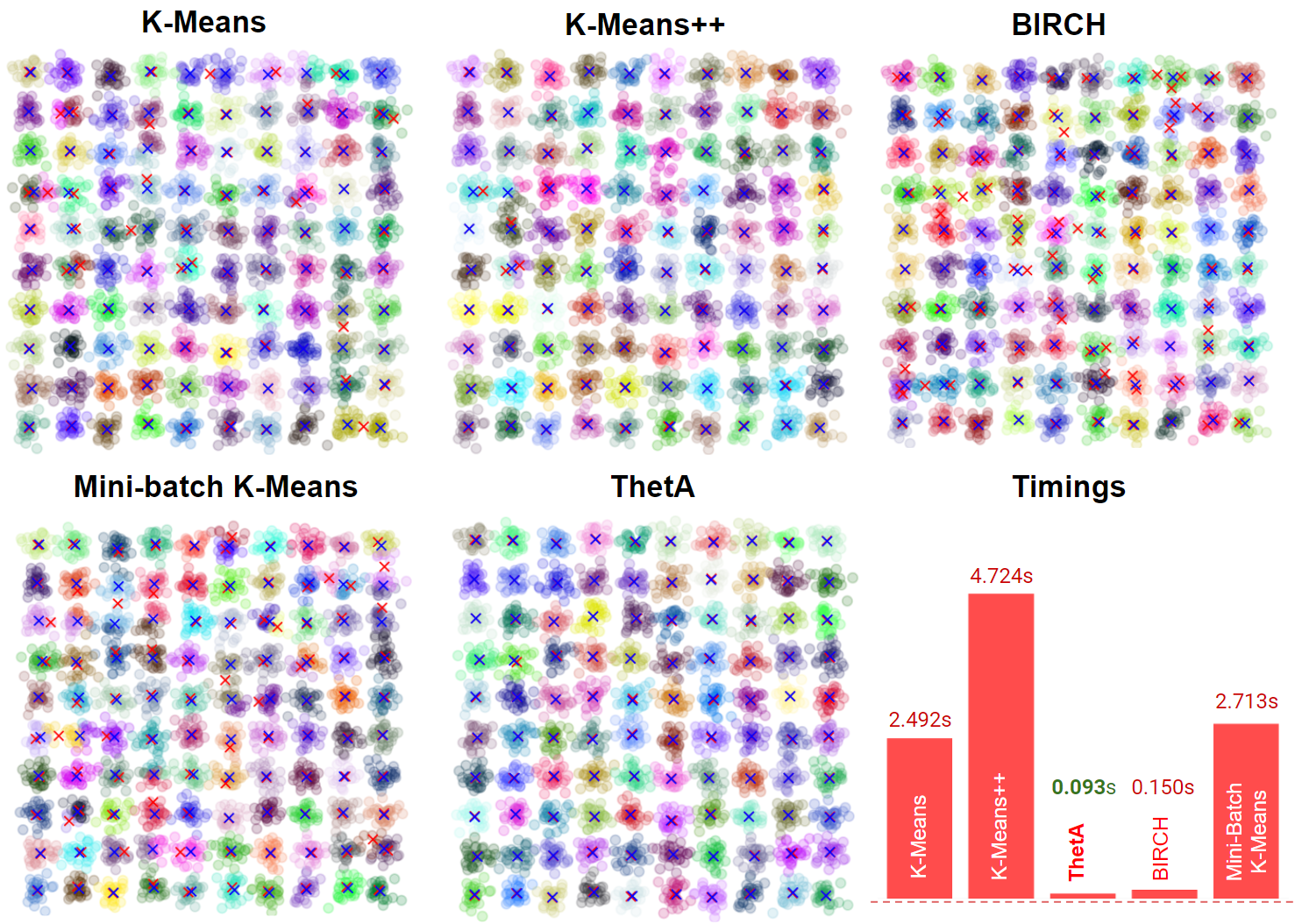

5.2 Hard Case
In the hard case experiment we have 100 clusters and each centroid has a short euclidean distance of 5 to each other. Unlike the easy case experiment, K-Means, K-Means++ and Mini-Batch K-Means were assigned 50 number of initializations additional to the number of clusters to match the advantage ThetA (TDG) would have by its multiple number of shuffles. BIRCH was run with threshold of 2.0 and branching factor of 50. ThetA used a threshold of 3.6 and 50 number of shuffles. The resulting Fig. 3 shows that now that the clusters are closer to each other, methods start to fail, while ThetA maintains its accuracy and speed advantage. It can also be seen in the supplementary section ThetA has a stable accuracy regardless of the difference in number of points per cluster, unlike other methods.
5.3 Change in number of dimensions
We provide box plots, as shown in Fig. 2 drawn from 10 runs of each case; 100 and 1000 number of dimensions with a fixed number of clusters set to 100. The experiments were done on the hard case, where the Manhattan distance difference between each consecutive cluster was set to where D is the number of dimensions, for consistency. The number of shuffles for TDG and number of initializations for K-Means, K-Means++ and Mini-batch K-Means were all set to 50. On 100 dimensions the conditions were threshold of 15.4 for ThetA and 12.75 for BIRCH and for 1000 dimension the thresholds were set to 50 and 29.96 for ThetA and BIRCH. The experiment with the change in number of clusters has been added to the supplement.
With higher number of dimensions, while the time taken for ThetA can be slower than some methods in higher dimensions (which is possibly because these algorithms converge faster to a local minimum solution rather to the global solution), we can see that the accuracy of TDG remains stable while other methods fluctuate or decrease.
5.4 Choice of Theta
In Fig. 4 we show an experiment to elucidate how the optimal value of theta change in relation to the distances between the clusters. We basically generated normal distributions on a grid and simply repeated TDG for different distance thresholds. Notice that we have a wide range of optimal that provide the correct number of cluster. Notice also the changes in optimal ranges of optimal given the sparsity of the dataset. As density increases, the range of optimal decrease, but there is still a relatively wide range of .
For the easy case it becomes trivial to learn the optimal and ordering is not a consideration but as the problem becomes harder the optimal becomes harder to find and the ordering problem becomes more severe. However, even in the case of a super dense problem we can use a lower value and study the sizes of the clusters. See example and comparisons using S1-4 datasets in Fig. 6. The distances between centroids were 11, 7.5 and 5 for each case.
5.5 Deep Embedded Clustering
We show how Algorithm 2 can facilitate and boost Deep Embedded Clustering (Xie et al. 2016) in a completely unsupervised way. We follow the paper’s base model architecture from training a simple Autoencoder model with 4 dense layers for the encoder and 4 dense layers for the decoder. For this application we use real data from the well studied MNIST dataset (LeCun et al. 1998). The method adds a clustering layer which uses the last layer of the encoder as a latent feature dimension input and produces soft labels using the Student t-distribution. KL divergence and Mean Squared Error loss are used for reconstruction and clustering loss. For comparison, we initialize the centroids in the clustering layer using three methods; K-Means, K-Means++ and TDG with threhold 4.724. Since there are many outliers that can be detected, we cluster more than 10 centroids using Algorithm 2 and use only the top 10 centroids that have the most samples in their cluster. As seen in Fig. 5, ThetA starts with a higher accuracy and NMI but also has a higher rate of increase through epochs. Note that this is not an experiment to show how the TDG performs using latent dimensions but to compare each method’s ability to cluster latent features.
5.6 Set-S dataset
We run TDG and K-Means++ on the Set-S dataset (Fränti & Virmajoki 2006). The dataset contains clusters of different shapes. We show how theta can correctly assign the clusters given an optimal threshold. Moreover, it also helps in inferring the number of clusters in each of S1-4 shown in Fig. 6. As seen in the line plot, there is a notable drop in the points per cluster after passing the correct number of clusters. We further elaborate on this observation in the case of Deep Embedded Clustering experiment where we can identify the correct number of clusters by using a threshold that creates more than the number of correct clusters. NMI table shows that the resulting clusters are closer to the ground truth than K-Means++. K-Means++ setup had 10 number of initializations with 300 max iterations. TDG was used with equal to for all S1 to S4 datasets.

6 Results Summary
Our results suggest that ThetA (TDG & TSG) tends to surpass other methods in terms of accuracy and complexity in both linearly separable easy and hard cases, regardless of the numbers of dimensions. Also, though not always faster than K-Means, the algorithm always takes less time than K-Means++, the only comparable method in the experiments that has a relatively close accuracy. Note that we compare against the Elkan’s method (Elkan 2003) for both K-Means and K-Means++ which is significantly faster than Lloyd’s algorithm. Also note that BIRCH is faster in convergence with respect to ThetA, however, it does not converge to the correct solution.
As seen in the choice of ThetA experiment, though the range of stable decrease as the problem gets harder, it still shows that there is a large enough region that predicts the correct number of clusters which makes it easier to learn the correct for ThetA algorithms to use.
It is also important to note that finding more than ground truth clusters through TDG can be easily solved by choosing only the centroids with the highest number of points in their clusters. The sharp drop in Fig. 6 suggests that this number and its corresponding is straightforward to learn.
7 Discussion

ThetA is a fast and robust unsupervised method as shown in the complexity analysis and experiments. This is an introductory paper to introduce new distance threshold based algorithms and propose using distance threshold rather than number of clusters for solving linear and in the future non-linear problems. There are still many ideas that can further improve ThetA, including workarounds to decrease the number of distance calculations. Techniques used by Elkan K-Means, Hamerly K-Means (Hamerly 2010) or parallelization can be all used to improve ThetA’s already fast execution time.
It is important to note that ThetA is very stable in terms of scaling. Sec. 5.3 shows this by increasing the number of dimensions and increasing the number of clusters. Additionally, our experiments show that the algorithms are less susceptible to datasets which have different number of points per cluster. These stable features of the algorithm reinforces our claim that ThetA should be used on biological and physical sciences data instead of other methods, not just because it uses only a distance threshold but also because of its stability. Experiments validating the claims can be seen in the main document and the supplementary sections.
In addition, TSG is equivalent to identifying the sparsity/density of datasets in high and low dimensions. If multiple iterations of TSG do not change the outcome then the dataset can be considered sparse. Otherwise, it would be a dense dataset.
There can be an ordering issue where TDG does not converge after multiple runs, which implies that correct clustering does not have a higher chosen rate. However, possibly a good solution can be generated by deploying a lower value and studying the cluster sizes as shown in Sec. 5.5 and 5.6.
The experiment on the MNIST Dataset using Deep Embedded Clustering with TDG has a remarkable accuracy of 94, considering the approach is completely unsupervised. Since other deep clustering approaches (Caron et al. 2018; Yang et al. 2017) also use K-Means as their clustering method, it is safe to assume that using ThetA will increase their performance likewise.
By proposing TDG and TNC, we for the first time show how the ordering problem persistent in such distance-threshold based algorithms can be tackled. We provide a short proof-sketch on Sec. 4.2 of how TDG improves the clustering accuracy by accounting for this issue. With a surge of interest in applying clustering to deep learning problems, we show how ThetA can be used to perform clustering in the latent space via Deep Embedded Clustering in Sec. 5.5 with an improved accuracy and cluster assignment. While all the experiments in this work were performed using the norm, future extension of this work would show that ThetA can be extended for other norms.
8 Conclusions
The problem of identifying the structure of high dimensional spaces is one that has occupied scientists for decades. In this work, we introduce a new family of algorithms called ThetA which enable the study of these high dimensional spaces and their sparsity in a principled way. In addition, we stress that ThetA outperforms the state of the art methods in linearly separable clustering problems both in speed and accuracy. We also provide guidelines of how these algorithms can be used for solving nonlinearly separable clustering problems and boosting the accuracy of unsupervised deep learning solutions.
References
- Aghabozorgi et al. (2015) Aghabozorgi, S., Shirkhorshidi, A. S., and Wah, T. Y. Time-series clustering–a decade review. Information Systems, 53:16–38, 2015.
- Agrawal & Agrawal (2015) Agrawal, S. and Agrawal, J. Survey on anomaly detection using data mining techniques. Procedia Computer Science, 60:708–713, 2015.
- Arthur & Vassilvitskii (2007) Arthur, D. and Vassilvitskii, S. k-means++ the advantages of careful seeding. In Proceedings of the eighteenth annual ACM-SIAM symposium on Discrete algorithms, pp. 1027–1035, 2007.
- Bradley & Fayyad (1998) Bradley, P. S. and Fayyad, U. M. Refining initial points for k-means clustering. In ICML, volume 98, pp. 91–99. Citeseer, 1998.
- Caron et al. (2018) Caron, M., Bojanowski, P., Joulin, A., and Douze, M. Deep clustering for unsupervised learning of visual features. In Proceedings of the European Conference on Computer Vision (ECCV), pp. 132–149, 2018.
- Elkan (2003) Elkan, C. Using the triangle inequality to accelerate k-means. In Proceedings of the 20th international conference on Machine Learning (ICML-03), pp. 147–153, 2003.
- Fränti & Virmajoki (2006) Fränti, P. and Virmajoki, O. Iterative shrinking method for clustering problems. Pattern Recognition, 39(5):761–765, 2006. doi: 10.1016/j.patcog.2005.09.012. URL http://dx.doi.org/10.1016/j.patcog.2005.09.012.
- Garyfallidis et al. (2012) Garyfallidis, E., Brett, M., Correia, M. M., Williams, G. B., and Nimmo-Smith, I. Quickbundles, a method for tractography simplification. Frontiers in neuroscience, 6:175, 2012.
- Hamerly (2010) Hamerly, G. Making k-means even faster. In Proceedings of the 2010 SIAM international conference on data mining, pp. 130–140. SIAM, 2010.
- Hartigan & Wong (1979) Hartigan, J. A. and Wong, M. A. Ak-means clustering algorithm. Journal of the Royal Statistical Society: Series C (Applied Statistics), 28(1):100–108, 1979.
- LeCun et al. (1998) LeCun, Y., Bottou, L., Bengio, Y., and Haffner, P. Gradient-based learning applied to document recognition. Proceedings of the IEEE, 86(11):2278–2324, 1998.
- Lloyd (1982) Lloyd, S. Least squares quantization in pcm. IEEE transactions on information theory, 28(2):129–137, 1982.
- Lu et al. (2015) Lu, J., Wu, D., Mao, M., Wang, W., and Zhang, G. Recommender system application developments: a survey. Decision Support Systems, 74:12–32, 2015.
- McFarland et al. (2015) McFarland, J. M., Bondy, A. G., Saunders, R. C., Cumming, B. G., and Butts, D. A. Saccadic modulation of stimulus processing in primary visual cortex. Nature communications, 6(1):1–14, 2015.
- Milligan & Cooper (1985) Milligan, G. W. and Cooper, M. C. An examination of procedures for determining the number of clusters in a data set. Psychometrika, 50(2):159–179, 1985.
- Patra et al. (2011) Patra, B. K., Nandi, S., and Viswanath, P. A distance based clustering method for arbitrary shaped clusters in large datasets. Pattern Recognition, 44(12):2862–2870, 2011.
- Pedregosa et al. (2011) Pedregosa, F., Varoquaux, G., Gramfort, A., Michel, V., Thirion, B., Grisel, O., Blondel, M., Prettenhofer, P., Weiss, R., Dubourg, V., Vanderplas, J., Passos, A., Cournapeau, D., Brucher, M., Perrot, M., and Duchesnay, E. Scikit-learn: Machine learning in Python. Journal of Machine Learning Research, 12:2825–2830, 2011.
- Rush & Russell (1988) Rush, M. C. and Russell, J. E. Leader prototypes and prototype-contingent consensus in leader behavior descriptions. Journal of Experimental Social Psychology, 24(1):88–104, 1988.
- Sculley (2010) Sculley, D. Web-scale k-means clustering. In Proceedings of the 19th international conference on World wide web, pp. 1177–1178, 2010.
- Theodoridis & Koutroumbas (2006) Theodoridis, S. and Koutroumbas, K. Pattern Recognition. Elsevier Science Limited, 2006.
- Ungar & Foster (1998) Ungar, L. H. and Foster, D. P. Clustering methods for collaborative filtering. In AAAI workshop on recommendation systems, volume 1, pp. 114–129. Menlo Park, CA, 1998.
- Xie et al. (2016) Xie, J., Girshick, R., and Farhadi, A. Unsupervised deep embedding for clustering analysis. In International conference on machine learning, pp. 478–487. PMLR, 2016.
- Xu & Wunsch (2010) Xu, R. and Wunsch, D. C. Clustering algorithms in biomedical research: a review. IEEE reviews in biomedical engineering, 3:120–154, 2010.
- Yang et al. (2017) Yang, B., Fu, X., Sidiropoulos, N. D., and Hong, M. Towards k-means-friendly spaces: Simultaneous deep learning and clustering. In international conference on machine learning, pp. 3861–3870. PMLR, 2017.
- Zhang et al. (1996) Zhang, T., Ramakrishnan, R., and Livny, M. Birch: an efficient data clustering method for very large databases. ACM sigmod record, 25(2):103–114, 1996.