Learning low-rank latent mesoscale structures in networksThanks: Our code for our algorithms and simulations is available at https://github.com/HanbaekLyu/NDL_paper. At https://github.com/jvendrow/Network-Dictionary-Learning, we provide a user-friendly version as a Python package ndlearn.
Abstract.
It is common to use networks to encode the architecture of interactions between entities in complex systems in the physical, biological, social, and information sciences. To study the large-scale behavior of complex systems, it is useful to examine mesoscale structures in networks as building blocks that influence such behavior [153, 154]. We present a new approach for describing low-rank mesoscale structures in networks, and we illustrate our approach using several synthetic network models and empirical friendship, collaboration, and protein–protein interaction (PPI) networks. We find that these networks possess a relatively small number of ‘latent motifs’ that together can successfully approximate most subgraphs of a network at a fixed mesoscale. We use an algorithm for ‘network dictionary learning’ (NDL) [155], which combines a network-sampling method [156] and nonnegative matrix factorization [157, 155], to learn the latent motifs of a given network. The ability to encode a network using a set of latent motifs has a wide variety of applications to network-analysis tasks, such as comparison, denoising, and edge inference. Additionally, using a new network denoising and reconstruction (NDR) algorithm, we demonstrate how to denoise a corrupted network by using only the latent motifs that one learns directly from the corrupted network.
It is often insightful to examine structures in networks [158] at intermediate scales (i.e., at ‘mesoscales’) that lie between the microscale of nodes and edges and the macroscale distributions of local network properties. Researchers have considered subgraph patterns (i.e., the connection patterns of subsets of nodes) as building blocks of network structure at various mesoscales [159]. In many studies of networks, researchers identify -node (where is typically between and ) subgraph patterns of a network that are unexpectedly common in comparison to some random-graph null model as ‘motifs’ of that network [160]. In the past two decades, the study of motifs has been important for the analysis of networked systems in many areas, including biology [161, 162, 163, 164, 165], sociology [166, 167], and economics [168, 169]. However, to the best of our knowledge, researchers have not examined how to use such motifs (or related mesoscale structures), after their discovery, as building blocks to reconstruct a network. In the present paper, we provide this missing computational framework to bridge inferred subgraph-based mesoscale structures and the global structure of networks. To do this, we propose (1) a ‘network dictionary learning’ (NDL) algorithm that learns ‘latent motifs’ from samples of certain random -node subgraphs and (2) a complementary algorithm for ‘network denoising and reconstruction’ (NDR) that constructs a best ‘mesoscale linear approximation’ of a given network using the learned latent motifs. We also provide a rigorous theoretical analysis of the proposed algorithms. This analysis includes a novel result in which we prove that one can accurately reconstruct an entire network if one has a dictionary of latent motifs that can accurately approximate mesoscale structures of the network. We compare our approach to related prior work [155] in the ‘Methods’ section and in our Supplementary Information (SI).
Using our approach, we find that various real-world networks (such as Facebook friendship networks, Coronavirus and Homo sapiens protein–protein interaction (PPI) networks, and an arXiv collaboration network) have low-rank subgraph patterns, in the sense that one can successfully approximate their -node subgraph patterns by a weighted sum of a small number of latent motifs. The latent motifs of these networks thereby reveal low-rank mesoscale structures of these networks. Our claim of the low-rank nature of such mesoscale structures concerns the space of certain subgraph patterns, rather than the embedding of an entire network into a low-dimensional Euclidean space (as considered in spectral-embedding and graph-embedding methods [170, 171]). It is impossible to obtain such a low-dimensional graph embedding for networks with small mean degrees and large clustering coefficients [172]. Additionally, as we demonstrate in this paper, the ability to encode a network using a set of latent motifs has a wide variety of applications in network analysis. These applications include network comparison, denoising, and edge inference.
Motivating application: Anomalous-subgraph detection
A common problem in network analysis is the detection of anomalous subgraphs of a network (see Figure 1) [173]. The connection pattern of an anomalous subgraph distinguishes it from the rest of a network. This anomalous-subgraph-detection problem has numerous high-impact applications, including in security, finance, healthcare, and law enforcement [174, 175]. Various approaches, including both classical techniques [173] and modern deep-neural-network techniques [176], have been proposed to detect anomalous subgraphs.

Consider the following simple conceptual framework for anomalous-subgraph detection.
- •
We learn “normal subgraph patterns” in an observed network and then seek to detect subgraphs in the observed network that deviate significantly from them.
By studying low-rank mesoscale structures in networks, we can turn this high-level idea for anomalous-subgraph detection into a concrete approach, which we now briefly summarize. First, we compute latent motifs (see Figure 1d) of an observed network (see Figure 1a) that can successfully approximate the -node subgraphs of the observed network. A key observation is that these subgraphs should also describe the normal subgraph patterns of the observed network (see Figure 1b). The rationale that underlies this observation is that the -node subgraphs of the observed network likely form a low-rank space, so we expect the latent motifs to be robust with respect to the addition of anomalous edges (see Figure 1c). Consequently, reconstructing the observed network using its latent motifs yields a weighted network (see Figure 1e) in which edges with positive and small weights deviate significantly from the normal subgraph patterns, which are captured by the latent motifs. Therefore, such edges are likely to be anomalous. The suspicious edges (see Figure 1f) are the edges in the weighted reconstruction that have positive weights that are less than a threshold. One can determine the threshold using a small set of known true edges and known anomalous edges. The suspicious edges match well with the anomalous edges in Figure 1c. See the SI for more details.
In the remainder of our paper, we carefully develop the three key components of our approach: (1) effective sampling of -node subgraphs; (2) reconstructing observed networks using candidate latent motifs; and (3) computing latent motifs from observed networks. The key idea of our work is to approximate sampled subgraphs by latent motifs and then combine these approximations to construct a weighted reconstructed network. We illustrate this procedure in Figure 3. We also present a variety of supporting numerical experiences using several synthetic and real-world networks.
-path motif sampling and latent motifs
Computing all -node subgraphs of a network is computationally expensive and is the main computational bottleneck of traditional motif analysis [160]. Our approach, which bypasses this issue, is to learn latent motifs by drawing random samples of a particular class of -node connected subgraphs. We consider random -node subgraphs that we obtain by uniformly randomly sampling a ‘-path’ from a network and including all edges between the sampled nodes of the network. A sequence of (not necessarily distinct) nodes is a -walk if and are adjacent for all . A -walk is a -path if all nodes in the walk are distinct (see Figure 2). Sampling a -path serves two purposes: (1) it ensures that the sampled -node induced subgraph is connected with the minimum number of imposed edges; and (2) it induces a natural node ordering of the -node induced subgraph. (Such an ordering is important for computations that involve subgraphs.) By using the ‘-walk’ motif-sampling algorithm in [156] in conjunction with rejection sampling, one can sample a large number of -paths and obtain their associated induced subgraphs.
The -node subgraphs that are induced by uniformly randomly sampling -paths from a network are the mesoscale structures that we consider in the present paper. We use the term ‘on-chain edges’ for the edges of these subgraphs between nodes and for , and we use the term ‘off-chain edges’ for all other edges. It is the off-chain edges that can differ across subgraphs and hence encode meaningful information about the network. For , the subgraphs are all isomorphic to a 2-path and hence have no off-chain edges. For , the subgraphs can have a single off-chain edge, so they are isomorphic either to a 2-path or to a 3-clique (i.e., a graph with three nodes and all three possible edges between them). For larger values of , the subgraphs can have diverse connection patterns (see Figure 2), depending on the architecture of the original network).
We study the connection patterns of a random -node subgraph by decomposing it as a weighted sum of more elementary subgraph patterns (possibly with continuous-valued edge weights), which we call latent motifs (see Figures 3a1–a3). To study mesoscale structures in networks, we investigate several questions. How many distinct latent motifs does one need to successfully approximate all of these -node subgraph patterns? What do they look like? How do these latent motifs differ for different networks?

Low-rank network reconstruction using latent motifs
Suppose that we have a network and two collections, and , of latent motifs. How can one determine which of the collections better describes the mesoscale structure of ? One can sample a large number of -node subgraphs of and, for each , independently, determine the nonnegative linear combination of latent motifs that yields the closest approximation . By comparing the subgraphs with their corresponding approximations , one can demonstrate how well the latent motifs in the ‘network dictionary’ approximates the -node subgraph patterns of (see Figures 3a1–a3).
For applications such as anomalous-subgraph detection, it is helpful to construct a weighted network with the same node set that gives the ‘best approximation’ of using the network dictionary . We regard the network as a ‘rank- mesoscale reconstruction’ of . If is close to , we conclude that the latent motifs in successfully capture the structure of -node subgraphs of and that has a rank- subgraph patterns that is prescribed by the latent motifs in . We interpret the edge weights in as measures of confidence in the corresponding edges in with respect to . For example, if an edge has the smallest weight in , we interpret it as the most ‘outlying’ edge with respect to the latent motifs in (see Figures 1e,f). We can threshold the weighted edges of at some fixed value to obtain an undirected reconstructed network with binary edge weights (which are either or ). We can then directly compare to the original unweighted network .
Our network denoising and reconstruction (NDR) algorithm (see Algorithm NDR in the SI) works as follows. We seek to build a weighted network using the node set and a weighted adjacency matrix . This network best approximates the observed network , whose subgraphs are generated by the latent motifs in . First, we uniformly randomly sample a large number of -paths in . We then determine the unweighted matrices with entries , which equals 1 if nodes and are adjacent in the network and equals 0 otherwise. These are the adjacency matrices of the induced subgraphs of the nodes of the -paths that we sampled (see Figure 3a2). We then approximate each by a nonnegative linear combination of the latent motifs in (see Figure 3a3). We then we compute for each as the mean of over all and all such that and (see Figure 3a4). We also provide theoretical guarantees and error bounds for our NDR algorithm in the SI (see Algorithm NDR).
Consider reconstructing a network using a single latent motif that is a -path. We begin with the case , such that each subgraph that we sample is a -path. The sampled -paths are approximated perfectly by (see Figure 3b1). A -path that one chooses uniformly at random has an equal probability of sampling each edge of , so . Therefore, we conclude that, at scale , one can perfectly reconstruct by using the -path latent motif . However, for , the graph can differ significantly from , as approximating the observed subgraphs by a single -path misses all of the off-chain edges (see Figures 3b1–b3). Therefore, to properly describe the -node subgraph patterns of , one may need more than one latent motif with off-chain edges (see Figure 3a3). We give more details in Appendix D of the SI.
Dictionary learning and latent motifs
How does one compute latent motifs from a given network? Dictionary-learning algorithms are machine-learning techniques that learn interpretable latent structures of complex data sets. They are employed regularly in the data analysis of text and images [177, 178, 179]. Dictionary-learning algorithms usually consist of two steps. First, one samples a large number of structured subsets of a data set (e.g., square patches of an image or collections of a few sentences of a text); we refer to such a subset as a mesoscale patch of a data set. Second, one finds a set of basis elements such that taking a nonnegative linear combination of them can successfully approximate each of the sampled mesoscale patches. Such a set of basis elements is called a dictionary, and one can interpret each basis element as a latent structure of the data set.

As an example, consider the artwork image in Figure 4a. We first uniformly randomly sample 10,000 square patches of pixels and vectorize them to obtain a matrix . The choice of vectorization is arbitrary; we use the column-wise vectorization in Algorithm A4 in the SI. We then use a nonnegative matrix factorization (NMF) [157] algorithm to find an approximate factorization , where and are nonnegative matrices of sizes and , respectively. Reshaping the columns of into square images yields an image dictionary that describes ‘latent shapes’ of the image.
Our network dictionary learning (NDL) algorithm to compute a ‘network dictionary’ that consists of latent motifs is based on a similar idea. As mesoscale patches of a network, we use the binary (i.e., unweighted) matrices that encode connection patterns between the nodes that form a uniformly random -path. After obtaining sufficiently many mesoscale patches of a network (e.g., by using a motif-sampling algorithm [156] with rejection sampling), we apply a dictionary-learning algorithm (e.g., NMF [157]) to obtain latent motifs of the network. A latent motif is a -node weighted network with nodes and edges that have weights between and . We use the term ‘on-chain edges’ for the edges of a latent motif between nodes and for ; we use the term ‘off-chain edges’ for all other edges. We give more background about our NDL algorithm in the ‘Methods’ section and provide a complete implementation of our approach in Algorithm NDL in the SI. We give theoretical guarantees for Algorithm NDL in Theorems F.4 and F.7 in the SI.
In Figure 4, we compare 25 latent motifs with nodes of Facebook friendship networks (which were collected on one day in fall 2005) from UCLA (‘UCLA’) and Caltech (‘Caltech’) [180, 181]. Each node in one of these networks is a Facebook account of an individual, and each edge encodes a Facebook friendship between two individuals. The latent motifs reveal striking differences between these networks in the connection patterns of the subgraphs that are induced by -paths with . For example, the latent motifs in UCLA’s dictionary (see Figure 4b) have sparse off-chain connections with a few clusters, whereas Caltech’s dictionary (see Figure 4c) has relatively dense off-chain connections. Most of Caltech’s latent motifs have ‘hub’ nodes (which are adjacent to many other nodes in the latent motif) or communities [182, 183] with six or more nodes. (See Figure 14 in the SI for community-size statistics.) An important property of -node latent motifs is that any network structure (e.g., hub nodes, communities, and so on) in the latent motifs must also exist in actual -node subgraphs. We observe both hubs and communities in the subgraphs samples from Caltech in Figure 2. By contrast, most of UCLA’s latent motifs do not have such structures, as is also the case for the subgraph samples from UCLA in Figure 2.
Because -node latent motifs encode basic connection patterns of nodes that are at most edges apart, one can interpret as a scale parameter. Latent motifs that one learns from the same network for different values of reveal different mesoscale structures. See Figure 13 in the SI for more details.
Example networks
We demonstrate our approach using 16 example networks; 8 of them are real-world networks and 8 of them synthetic networks. The 8 real-world networks are Coronavirus PPI (for which we use the shorthand Coronavirus) [184, 185, 186] and Homo sapiens PPI (for which we use the shorthand H. sapiens) [184, 171]; Facebook networks from Caltech, UCLA, Harvard, and MIT [180, 181]; SNAP Facebook (for which we use the shorthand SNAP FB) [187, 171]; and arXiv ASTRO-PH (for which we use the shorthand arXiv) [188, 171]. The first network is a protein–protein interaction (PPI) network of proteins that are related to the coronaviruses that cause Coronavirus disease 2019 (COVID-19), Severe Acute Respiratory Syndrome (SARS), and Middle Eastern Respiratory Syndrome (MERS) [185]. The second network is a PPI network of proteins that are related to Homo sapiens [184]. The third network is a 2012 Facebook network that was collected from participants in a survey [187]. The fourth network is a collaboration network from coauthorships of preprints that were posted in the astrophysics category of the arXiv preprint server. The last four real-world networks are 2005 Facebook networks from four universities from the Facebook100 data set [181]. In each Facebook network, nodes represent accounts and edges encode Facebook ‘friendships’ between these accounts.
For the eight synthetic networks, we generate two instantiations each of Erdős–Rényi (ER) networks [189], Watts–Strogatz (WS) networks [190], Barabási–Albert (BA) networks [191], and stochastic-block-model (SBM) networks [192]. These four random-graph models are well-studied and are common choices for testing new network methods and models [158]. Each of the ER networks has 5,000 nodes, and we independently connect each pair of nodes with probabilities of (in the network that we call ER1) and (in ER2). For the WS networks, we use rewiring probabilities of (in WS1) and (in WS2) starting from a 5,000-node ring network in which each node is adjacent to its nearest neighbors. For the BA networks, we use (in BA1) and (in BA2), where denotes the number of edges of each new node when it connects (via linear preferential attachment) to the existing network, which we grow from an initial network of isolated nodes (i.e., none of them are adjacent to any other node) until it has 5,000 nodes. The SBM networks SBM1 and SBM2 have three planted 1,000-node communities; two nodes in the th and the th communities are connected by an edge independently with probability if (i.e., if they are in the same community) and for SBM1 and for SBM2 if (i.e., if they are in different communities). See the ‘Methods’ section for more details.
Network-reconstruction experiments
An important observation is that one can reconstruct a given network using an arbitrary network dictionary, including ones that one learns from an entirely different network. Such a ‘cross-reconstruction’ allows one to quantitatively compare the learned mesoscale structures of different networks. In Figure 5, we show the results of several network-reconstruction experiments using a variety of real-world networks and synthetic networks. We label each subplot of Figure 5 with to indicate that we are reconstructing network by approximating mesoscale patches of using a network dictionary that we learn from network . We perform these experiments for various values of the edge threshold and latent motifs in a single dictionary. Each network dictionary in Figure 5 has nodes, for which the dimension of the space of all possible mesoscale patches (i.e., the adjacency matrices of the induced subgraphs) is . We measure the reconstruction accuracy by calculating the Jaccard index between the original network’s edge set and the reconstructed network’s edge set. That is, to measure the similarity of two edge sets, we calculate the number of edges in the intersection of these sets divided by the number of edges in the union of these sets. This gives a measure of reconstruction accuracy; if the Jaccard index equals , the reconstructed network is precisely the same as the original network. We obtain the same qualitative results as in Figure 5 if we instead measure similarity using the Rand index [193]).

In Figure 5a, we plot the accuracy of the ‘self-reconstruction’ versus the threshold (with latent motifs), where is one of the real-world networks Coronavirus, H. sapiens, SNAP FB, Caltech, and arXiv. The accuracies for Coronavirus, H. sapiens, and Caltech peak above when ; the accuracies for arXiv and SNAP FB peak above and , respectively, for . We choose for the cross-reconstruction experiments for the Facebook networks Caltech, Harvard, MIT, and UCLA in Figures 5b,c. These four Facebook networks have self-reconstruction accuracies above for motifs with a threshold of . The total number of dimensions when using mesoscale patches at scale is , so this result suggests that all eight of these real-world networks have low-rank mesoscale structures at scale .

We gain further insights into our self-reconstruction experiments by comparing the degree distributions and the mean local clustering coefficients of the original and the unweighted reconstructed networks with threshold (see Figure 6). The mean local clustering coefficients of all reconstructed networks are similar to those of the corresponding original networks. In Figure 6a, we show that the degree distributions of the reconstructed networks for Caltech with latent motifs converge toward that of the original network as we increase . Reconstructing Caltech with larger values of appears to increase accuracy by including nodes with a larger degree than is possible for smaller values of . In other words, ‘low-rank’ reconstructions (i.e., those with small values of ) of Caltech seem to recover only a small number of the edges of each node, even though it is able to achieve a large reconstruction accuracy (e.g., over % for ).
We now consider cross-reconstruction accuracies in Figures 5b,c, where is one of the Facebook networks Caltech, Harvard, MIT, and UCLA and (with ) is one of the these four networks or one of the four synthetic networks ER2, WS2, BA2, and SBM2. From the cross-reconstruction accuracies and examining the network structures of the the latent motifs (see Appendix A.4 of the SI) in Figures 4 and 13 (also see Figures 18, 20, and 21 in the SI), we draw a few conclusions at scale . First, the mesoscale structure of Caltech is distinct from those of Harvard, UCLA, and MIT. This is consistent with prior studies of these networks (see, e.g., [181, 194]). Second, Caltech’s mesoscale structures at scale are higher-dimensional than those of the other three universities’ Facebook networks. Third, Caltech has a lot more communities with at least nodes than the other three universities’ Facebook networks (also see Figure 14). Fourth, the BA network BA2 captures the mesoscale structure of MIT, Harvard, and UCLA at scale better than the synthetic networks that we generate from the ER, WS, and SBM models. However, for all , the network SBM2 captures the mesoscale structures of Caltech better than all other networks in Figure 5b except for Caltech itself. See Appendix E.5 of the SI for further discussion.

We also comment briefly about the cross-reconstruction experiments in Figure 5 that use latent motifs that we learn from ER networks. For instance, when reconstructing MIT, Harvard, and UCLA using latent motifs that we learn from ER2, we obtain a reconstruction accuracy of at least 72%. This may seem unreasonable at first glance because the latent motifs that we learn from ER2 should not have any information about the Facebook networks. However, all of these networks are sparse (with edge densities of at most ) and we are sampling subgraphs using -paths. The -node subgraphs that are induced by uniformly random -paths in these sparse networks have only a few off-chain edges (see Figure 2). For example, the -node subgraphs that we sample from the sparse ER network ER2 tend to have -node paths and a few extra off-chain edges (see Figure 2). A similarly sparse or sparser network, such as UCLA (whose edge density is about ) has similar subgraph patterns (despite the fact that, unlike the subgraphs of ER2, the off-chain edges are not independent). This is the reason that we can reconstruct some networks with high accuracy by using latent motifs that we learn from a completely unrelated network.
One learns latent motifs by maximizing the accuracy of reconstructions of mesoscale patches using them, rather than by maximizing the network-reconstruction accuracy. In Figure 7b–e, we illustrate that self-reconstruction of mesoscale patches is more accurate than cross-reconstructions of mesoscale patches. However, because network reconstruction involves taking the mean of the reconstructed weights of an edge from multiple mesoscale patches that include that edge, an accurate reconstruction of mesoscale patches need not always entail accurate network reconstruction. In Figure 5, we see that the self-reconstruction is more accurate than the cross-reconstructions for for almost all choices of networks and and the parameter . The two exceptions are and , although the cross-reconstruction accuracies in these cases are at most larger than the self-reconstruction accuracy.
The above discussion suggests an important question: If a network dictionary is effective at approximating the mesoscale patches of a network, what reconstruction accuracy does one expect? In the present paper, we state and prove a novel theorem that answers this question. Specifically, we prove mathematically that a Jaccard reconstruction error of a weighted reconstructed network (i.e., without thresholding edge weights as in Figure 5) is upper-bounded by the mean approximation error of the mesoscale patches (i.e., -node subgraphs) of a network by the -path latent motifs divided by . See Appendix F.3 and Theorem F.4 in the SI for precise statements of the relevant definitions and the mathematical result.
Our NDL algorithm (see Algorithm NDL) finds a network dictionary that approximately minimizes the upper bound in the inequality in Figure 7a. (See Theorem F.4 in the SI.) Using an arbitrary network dictionary is likely to yield larger values of the upper bound. Therefore, according to the theorem in Figure 7a, it is likely to yield a less accurate weighted reconstructed network. For instance, for a network dictionary that consists of a single -path, the aforementioned upper bound is the mean number of off-chain edges in the mesoscale patches of a network divided by . (See the inequality in Figure 7a.) For an ER network with expected edge density , this upper bound equals in expectation. At scale for ER2, this value is . Consequently, we expect a reconstruction accuracy of at least when reconstructing ER2 using latent motifs (such as the ones for UCLA in Figure 4) that have large on-chain entries and small off-chain entries. Substituting the edge density of UCLA for , we expect a reconstruction accuracy of at least 94%. However, according to the first inequality in Figure 7a, the lower bound of the reconstruction accuracy that we obtain using latent motifs of UCLA is about 80%. Therefore, for UCLA, we expect to obtain many more off-chain edges in mesoscale patches than what we expect from an ER network with the same edge density. We plot the lower bound of the reconstruction accuracy in Figures 7b–e for the parameters in Figures 5b–e (i.e., and ). The lower bounds for the self-reconstructions is not too far from the actual reconstruction accuracies for unweighted reconstructed networks in Figures 5b–e (it is within % for Caltech and UCLA and within % for MIT and Harvard for all ), but we observe much larger accuracy gaps for the cross-reconstruction experiments. (For example, there is at least a % difference for UCLACaltech.) This indicates that, even if one uses latent motifs that are not very efficient at approximating mesoscale patches, one can obtain unweighted reconstructions that are significantly more accurate than what is guaranteed by the theoretically proven bounds.
Network-denoising experiments
We consider the following ‘network-denoising’ problem (which is closely related to the anomalous-subgraph-detection problem in Figure 1). Suppose that we are given an observed network with a node set and edge set and that we are asked to find an unknown network with the same node set but a possibly different edge set . We interpret as a corrupted version of a ‘true network’ that we observe with some uncertainty. To simplify the setting, we consider two types of network denoising. In the first type of network denoising, we consider additive noise [174, 195, 175, 196]. We suppose that is a corrupted version of that includes false edges (i.e., ), and we seek to classify all edges in into ‘positives’ (i.e., edges in ) and ‘negatives’ (i.e., false edges in or equivalently nonedges in ). This network-denoising setting is identical to the anomalous-subgraph-detection problem in Figure 1, except that now we label the false edges as negatives. We interpreted them as positives when we computed the F-score (i.e., the harmonic mean of the precision and recall scores) in Figure 1f. In the second type of network denoising, we consider subtractive noise (which is often called edge ‘prediction’ [197, 198, 199, 200, 201]). We assume that is a partially observed version of (i.e., ), and we seek to classify nonedges in into positives (i.e., nonedges in ) and negatives (i.e., edges in ). There are many more positives than negatives because is sparse (i.e., the edge density is low), so we restrict the classification task to a subset of that includes all negatives and an equal number of positives. We will discuss shortly how we choose .
Given a true network , we generate an observed (i.e., corrupted) network as follows. In the additive-noise setting, we create two types of corrupted networks. We create the first type of corrupted network by adding false edges in a structured way by generating them using the WS model. We select 100 nodes for four of the networks (the exception is that we use 500 nodes for H. sapiens) uniformly at random and generate 1,000 new edges (we generate 30,000 new edges for H. sapiens) according to the WS model. In this corrupting WS network, each node in a ring of 100 nodes is adjacent to its 20 nearest neighbors and we uniformly randomly choose 30% of the edges to rewire. When rewiring an edge, we choose between its two ends with equal probability of each, and we attach this end to a node in the network that we choose uniformly at random. We then add these newly generated edges to the original network. We refer to this noise type as ‘’. We create the second type of corrupted network by first choosing 5% of the nodes uniformly at random and adding an edge between each pair of chosen nodes with independent probability . We refer to this noise type as ‘’. In the subtractive-noise setting, we obtain from by removing half of the existing edges, which we choose uniformly at random, such that the remaining network is connected. We refer to this noise type as ‘’.
For each observed network , we apply NDL at scale with to learn a network dictionary . We construct another network dictionary by removing the on-chain edges from all of the latent motifs in . (See the ‘Methods’ section for further discussion.) This gives a total of four network dictionaries, corresponding to the two values of and whether or not we keep the on-chain edges of the latent motifs. With each of the network dictionaries, use NDR to reconstruct a network by approximating mesoscale patches of using latent motifs in . (We compute without using any information on .) We anticipate that the reconstructed network is similar to its corresponding original (i.e., uncorrupted) network . The reconstruction algorithms output a weighted network , where the weight of each edge is our confidence that the edge is a true edge of that network. For denoising subtractive (respectively, additive) noise, we classify each nonedge (respectively, each edge) in a corrupted network as ‘positive’ if its weight in is strictly larger than some threshold and as ‘negative’ otherwise. By varying , we construct a receiver-operating characteristic (ROC) curve that consists of points whose horizontal and vertical coordinates are the false-positive rates and true-positive rates, respectively. For denoising the (respectively, and ) noise, one can also infer an optimal value of for a 50% training set of nonedges (respectively, edges) of with known labels and then use this value of to compute classification measures such as accuracy and precision.
In Figure 8, we compare the performance of our network-denoising approach to the performance of several existing approaches using the real-world networks Caltech, SNAP FB, arXiv, Coronavirus, and H. sapiens. We use four classical approaches (the Jaccard index, preferential attachment, the Adamic–Adar index, and a spectral embedding) [198, 202] and two more recent methods (DeepWalk [170] and node2vec [171]) that are based on network embeddings. Let denote the set of neighbors of node of a network. For the Jaccard index, preferential attachment, and the Adamic–Adar index, the confidence score (which plays the same role as an edge weight in a reconstructed network) that the nodes and are adjacent via a true edge is , , and , respectively.
We now discuss how we choose the set of nonedges of for our subtractive-noise experiments. First, we note that it is unlikely that many deleted edges in are between two small-degree nodes. If we simply choose as a uniformly random subset of the set of all nonedges of with a given size , then it is likely that we will choose many nonedges between small-degree nodes. Consequently, the resulting classification problem is easy for existing methods, such as the Jaccard index and preferential attachment, that are based on node degrees. (For example, consider a star network with five leaves (i.e., degree-1 nodes). In this network, a uniformly randomly chosen nonedge is always attached to two degree-1 nodes, but a uniformly randomly chosen edge is always attached to one degree-5 node (i.e., the center node) and one degree-1 node.) To reduce the size-biasing of node degrees, we choose each nonedge of with a probability that is proportional to the product of the degrees of the two associated nodes.
We show results in the form of means of the areas under the curves (AUCs) of the ROC curves for five independent runs of each approach. In Figure 8, we see that our approach performs competitively in all of our experiments, particularly for denoising additive noise (i.e., anomalous-subgraph detection). For example, when we add 1,000 false edges that we generate from the WS model to Coronavirus (which has 2,463 true edges), our approach yields an AUC of . We obtain the second best AUC (of only ) using preferential attachment. For noise of type , we add false edges to Coronavirus; our approach achieves the best AUC (of ) and spectral embedding achieves the second best AUC (of ).
In Figure 5a, we saw that we can use a small number of latent motifs to reconstruct the social and PPI networks that we use for our denoising experiments in Figure 8. Because NDL learns a small number of latent motifs that are able to successfully give an approximate basis for all mesoscale patches, they should not be affected significantly by false edges between nodes in a small subset of the entire node set. Consequently, the latent motifs in that we learn from the observed network may still be effective at approximating mesoscale patches of the true network , so the network that we reconstruct using and may be similar to .
Conclusions and outlook
We introduced a mesoscale network structure, which we call latent motifs, that consists of -node subgraphs that are building blocks of all connected -node subgraphs of a network. In contrast to ordinary motifs [160], which refer to overrepresented -node subgraphs (especially for small ) of a network, nonnegative linear combinations of our latent motifs approximate -node subgraphs that are induced by uniformly random -paths in a network. We also established algorithmically and theoretically that one can approximate a network accurately if one has a dictionary of latent motifs that can accurately approximate mesoscale structures in the network.
Our computational experiments in Figures 4 and 13 demonstrated that latent motifs can have distinctive network structures. Our computational experiments in Figures 5, 11, and 8 illustrated that various social, collaboration, and PPI networks have low-rank [203] mesoscale structures, in the sense that a few latent motifs (e.g., of them, but see Figure 5 for other choices of ) that we learn using NDL are able to reconstruct, infer, and denoise the edges of a network using our NDR algorithm. We hypothesize that such low-rank mesoscale structures are a common feature of networks beyond the social, collaboration, and PPI networks that we examined. As we have illustrated in this paper, one can leverage mesoscale structures to perform important tasks like network denoising, so it is important in future studies to explore the level of generality of our insights.
In our work, we examined latent motifs in ordinary graphs. However, notions of motifs have been developed for several more general types of networks, including temporal networks (in which nodes, edges, and edge weights can change with time) [204] and multilayer networks (in which, e.g., nodes can be adjacent via multiple types of relationships) [205]. We did not consider latent motifs in such network structures, and it is worthwhile to extend our approach and algorithms to these situations.
Limitations and further discussion
In the next few paragraphs, we briefly discuss several salient points about our work.
First, it is possible for two sets of latent motifs to be equally effective at reconstructing the same network. Therefore, although one can interpret the structures in latent motifs as mesoscale structures of a network, one cannot conclude that other mesoscale structures (which not in a given set of latent motifs) do not also occur in the network.
Second, our NDL algorithm approximately computes a ‘best’ network dictionary to reconstruct the mesoscale patches of a network, rather than one to reconstruct the network itself. Although our theoretical bound on the reconstruction error (see Figure 7a) implies that such a network dictionary should also be effective at reconstructing a network, it is still necessary to empirically verify the actual efficacy of doing so.
Third, the same theoretical bound on the reconstruction error illustrates that it is possible to successfully reconstruct a very sparse network using latent motifs that one learns from a radically different but similarly sparse network at a given scale (see Figure 5e). To better distinguish distinct sparse networks from each other, one can use a scale that is large enough so that -node mesoscale patches have many off-chain edges and latent motifs at that scale are sufficiently different in different networks. For example, see the latent motifs at scale in Figures 18–21 in the SI. Naturally, using a larger scale increases the computational cost of our approach.
Fourth, although our method for network denoising is competitive — especially for the anomalous-subgraph-detection problem — it does not always outperform all existing methods, and some of those methods are much simpler than ours. For instance, for edge-prediction tasks, it seems that our method is often more conservative than the other examined methods at detecting unobserved edges. (See Figures 15, 16, and 17 in the SI.) Therefore, we recommend using our method in conjunction with existing methods for such tasks.
Acknowledgements
HL was supported by the National Science Foundation through grants 2206296 and 2010035. JV was supported by the National Science Foundation through grant 1740325.
LEARNING LOW-RANK LATENT MESOSCALE STRUCTURES IN NETWORKS
References
- [1] Jukka-Pekka Onnela et al. “Taxonomies of networks from community structure” In Physical Review E 86.3 APS, 2012, pp. 036104
- [2] Ankit. Khambhati, Ann. Sizemore, Richard. Betzel and Danielle. Bassett “Modeling and interpreting mesoscale network dynamics” In NeuroImage 180 Elsevier, 2018, pp. 337–349
- [3] Hanbaek Lyu, Deanna Needell and Laura Balzano “Online matrix factorization for Markovian data and applications to network dictionary learning” In Journal of Machine Learning Research 21, 2020, pp. 1–49
- [4] Hanbaek Lyu, Facundo Memoli and David Sivakoff “Sampling random graph homomorphisms and applications to network data analysis” In Journal of Machine Learning Research 24, 2023, pp. 1–79
- [5] Daniel. Lee and H. Seung “Learning the parts of objects by non-negative matrix factorization” In Nature 401.6755 Nature Publishing Group, 1999, pp. 788–791
- [6] Mark E.. Newman “Networks” Oxford, UK: Oxford University Press, 2018
- [7] Alice. Schwarze and Mason. Porter “Motifs for processes on networks” In SIAM Journal on Applied Dynamical Systems 20.4, 2021, pp. 2516–2557
- [8] Ron Milo et al. “Network motifs: Simple building blocks of complex networks” In Science 298.5594 American Association for the Advancement of Science, 2002, pp. 824–827
- [9] Gavin. Conant and Andreas Wagner “Convergent evolution of gene circuits” In Nature Genetics 34.3 Nature Publishing Group, 2003, pp. 264–266
- [10] Jason M.. Rip, Kevin. McCann, Denis. Lynn and Sonia Fawcett “An experimental test of a fundamental food web motif” In Proceedings of the Royal Society B: Biological Sciences 277.1688 The Royal Society, 2010, pp. 1743–1749
- [11] Olaf Sporns, Rolf K\"otter and Karl. Friston “Motifs in brain networks” In PLoS Biology 2.11 Public Library of Science San Francisco, USA, 2004, pp. e369
- [12] Konstantin Ristl, Sebastian. Plitzko and Barbara Drossel “Complex response of a food-web module to symmetric and asymmetric migration between several patches” In Journal of Theoretical Biology 354 Elsevier, 2014, pp. 54–59
- [13] Uri Alon “Network motifs: Theory and experimental approaches” In Nature Reviews Genetics 8.6 Nature Publishing Group, 2007, pp. 450–461
- [14] Xu Hong-lin, Yan Han-bing, Gao Cui-fang and Zhu Ping “Social network analysis based on network motifs” In Journal of Applied Mathematics 2014 Hindawi, 2014, pp. 874708
- [15] Krzysztof Juszczyszyn, Przemyslaw Kazienko and Bogdan Gabrys “Temporal changes in local topology of an email-based social network” In Computing and Informatics 28.6, 2009, pp. 763–779
- [16] Takaaki Ohnishi, Hideki Takayasu and Misako Takayasu “Network motifs in an inter-firm network” In Journal of Economic Interaction and Coordination 5.2 Springer, 2010, pp. 171–180
- [17] Frank. Takes, Walter. Kosters, Boyd Witte and Eelke. Heemskerk “Multiplex network motifs as building blocks of corporate networks” In Applied Network Science 3.1 Springer, 2018, pp. 39
- [18] Bryan Perozzi, Rami Al-Rfou and Steven Skiena “DeepWalk: Online learning of social representations” In Proceedings of the 20th ACM SIGKDD International Conference on Knowledge Discovery and Data Mining, 2014, pp. 701–710
- [19] Aditya Grover and Jure Leskovec “node2vec: Scalable feature learning for networks” In Proceedings of the 22nd ACM SIGKDD International Conference on Knowledge Discovery and Data Mining, 2016, pp. 855–864
- [20] C. Seshadhri, Aneesh Sharma, Andrew Stolman and Ashish Goel “The impossibility of low-rank representations for triangle-rich complex networks” In Proceedings of the National Academy of Sciences of the United States of America 117.11 National Academy of Sciences, 2020, pp. 5631–5637
- [21] Leman Akoglu, Hanghang Tong and Danai Koutra “Graph based anomaly detection and description: A survey” In Data Mining and Knowledge Discovery 29 Springer, 2015, pp. 626–688
- [22] Caleb. Noble and Diane. Cook “Graph-based anomaly detection” In Proceedings of the Ninth ACM SIGKDD International Conference on Knowledge Discovery and Data Mining, 2003, pp. 631–636
- [23] Benjamin. Miller, Michelle. Beard, Patrick. Wolfe and Nadya. Bliss “A spectral framework for anomalous subgraph detection” In IEEE Transactions on Signal Processing 63.16 IEEE, 2015, pp. 4191–4206
- [24] Xiaoxiao Ma et al. “A comprehensive survey on graph anomaly detection with deep learning” In IEEE Transactions on Knowledge and Data Engineering IEEE, 2021
- [25] Michael Elad and Michal Aharon “Image denoising via sparse and redundant representations over learned dictionaries” In IEEE Transactions on Image Processing 15.12 IEEE, 2006, pp. 3736–3745
- [26] Julien Mairal, Michael Elad and Guillermo Sapiro “Sparse representation for color image restoration” In IEEE Transactions on Image Processing 17.1 IEEE, 2007, pp. 53–69
- [27] Gabriel Peyr\’e “Sparse modeling of textures” In Journal of Mathematical Imaging and Vision 34.1 Springer, 2009, pp. 17–31
- [28] Veronica Red, Eric. Kelsic, Peter. Mucha and Mason. Porter “Comparing community structure to characteristics in online collegiate social networks” In SIAM Review 53, 2011, pp. 526–543
- [29] Amanda. Traud, Peter. Mucha and Mason. Porter “Social structure of Facebook networks” In Physica A 391.16 Elsevier, 2012, pp. 4165–4180
- [30] Mason. Porter, Jukka-Pekka Onnela and Peter. Mucha “Communities in networks” In Notices of the American Mathematical Society 56.9, 2009, pp. 1082–1097, 1164–1166
- [31] Santo Fortunato and Darko Hric “Community detection in networks: A user guide” In Physics Reports 659 Elsevier, 2016, pp. 1–44
- [32] Rose Oughtred et al. “The BioGRID interaction database: 2019 update” In Nucleic Acids Research 47.D1 Oxford University Press, 2019, pp. D529–D541
- [33] theBiogrid.org “Coronavirus PPI network” Retrieved from https://wiki.thebiogrid.org/doku.php/covid (downloaded 24 July 2020, Ver. 3.5.187.tab3), 2020
- [34] David. Gordon et al. “A SARS-CoV-2 protein interaction map reveals targets for drug repurposing” In Nature 583 Nature Publishing Group, 2020, pp. 1–13
- [35] Jure Leskovec and Julian. McAuley “Learning to discover social circles in ego networks” In Proceedings of the 25th International Conference on Neural Information Processing Systems — Volume 1, 2012, pp. 539–547
- [36] Jure Leskovec and Andrej Krevl “SNAP Datasets: Stanford Large Network Dataset Collection” Available at http://snap.stanford.edu/data, 2020
- [37] Paul Erdos and Alfr\’ed R\’enyi “On random graphs. I” In Publicationes Mathematicae 6.18, 1959, pp. 290–297
- [38] Duncan. Watts and Steven. Strogatz “Collective dynamics of ‘small-world’ networks” In Nature 393.6684 Nature Publishing Group, 1998, pp. 440–442
- [39] Albert-L\’aszl\’o Barab\’asi and R\’eka Albert “Emergence of scaling in random networks” In Science 286.5439 American Association for the Advancement of Science, 1999, pp. 509–512
- [40] Paul. Holland, Kathryn Laskey and Samuel Leinhardt “Stochastic blockmodels: First steps” In Social Networks 5.2 Elsevier, 1983, pp. 109–137
- [41] William. Rand “Objective criteria for the evaluation of clustering methods” In Journal of the American Statistical Association 66.336 Taylor & Francis Group, 1971, pp. 846–850
- [42] Lucas G.. Jeub et al. “Think locally, act locally: Detection of small, medium-sized, and large large networks” In Physical Review E 91.1 American Physical Society, 2015, pp. 012821
- [43] Rajul Parikh et al. “Understanding and using sensitivity, specificity and predictive values” In Indian Journal of Ophthalmology 56.1 Wolters Kluwer–Medknow Publications, 2008, pp. 45
- [44] Fernanda. Correia, Edgar. Coelho, Jos\’e. Oliveira and Joel. Arrais “Handling noise in protein interaction networks” In BioMed Research International 2019 Hindawi, 2019, pp. 8984248
- [45] Tao Zhou “Progresses and challenges in link prediction” In iScience 24.11, 2021, pp. 103217
- [46] David Liben-Nowell and Jon Kleinberg “The link-prediction problem for social networks” In Journal of the American Society for Information Science and Technology 58.7 Wiley Online Library, 2007, pp. 1019–1031
- [47] Aditya Menon and Charles Elkan “Link prediction via matrix factorization” In Machine Learning and Knowledge Discovery in Databases Heidelberg, Germany: Springer-Verlag, 2011, pp. 437–452
- [48] Istv\’an. Kov\’acs et al. “Network-based prediction of protein interactions” In Nature Communications 10.1 Nature Publishing Group, 2019, pp. 1240
- [49] Roger Guimer\‘a “One model to rule them all in network science?” In Proceedings of the National Academy of Sciences of the United States of America 117.41 National Acad Sciences, 2020, pp. 25195–25197
- [50] Mohammad Hasan and Mohammed. Zaki “A survey of link prediction in social networks” In Social Network Data Analytics Springer, 2011, pp. 243–275
- [51] Ivan Markovsky and Konstantin Usevich “Low Rank Approximation” Heidelberg, Germany: Springer-Verlag, 2012
- [52] Ashwin Paranjape, Austin Benson and Jure Leskovec “Motifs in temporal networks” In Proceedings of the Tenth ACM International Conference on Web Search and Data Mining, 2017, pp. 601–610
- [53] Federico Battiston, Vincenzo Nicosia, Mario Chavez and Vito Latora “Multilayer motif analysis of brain networks” In Chaos: An Interdisciplinary Journal of Nonlinear Science 27.4 AIP Publishing LLC, 2017, pp. 047404
- [54] Daniel. Lee and H. Seung “Algorithms for non-negative matrix factorization” In Proceedings of the 13th International Conference on Neural Information Processing Systems, 2001, pp. 556–562
- [55] Julien Mairal, Francis Bach, Jean Ponce and Guillermo Sapiro “Online learning for matrix factorization and sparse coding” In Journal of Machine Learning Research 11, 2010, pp. 19–60
- [56] Julien Mairal, Michael Elad and Guillermo Sapiro “Sparse learned representations for image restoration” In Proceedings of the 4th World Conference of the International Association for Statistical Computing, 2008, pp. 118 IASC
- [57] Julien Mairal et al. “Non-local sparse models for image restoration” In 2009 IEEE 12th International Conference on Computer Vision, 2009, pp. 2272–2279 IEEE
- [58] theBiogrid.org “Homo sapiens PPI network” Retrieved from https://wiki.thebiogrid.org/doku.php/covid (downloaded 24 July 2020, Ver. 3.5.180.tab2), 2020
- [59] L\’aszl\’o Lov\’asz “Large Networks and Graph Limits” 60, Colloquium Publications Providence, RI, USA: American Mathematical Society, 2012, pp. 475
- [60] Marco Bressan “Efficient and near-optimal algorithms for sampling connected subgraphs” In Proceedings of the 53rd Annual ACM SIGACT Symposium on Theory of Computing, STOC 2021 Virtual, Italy: Association for Computing Machinery, 2021, pp. 1132–1143
- [61] Nadav Kashtan, Shalev Itzkovitz, Ron Milo and Uri Alon “Efficient sampling algorithm for estimating subgraph concentrations and detecting network motifs” In Bioinformatics 20.11 Oxford University Press, 2004, pp. 1746–1758
- [62] Sebastian Wernicke “Efficient detection of network motifs” In IEEE/ACM Transactions on Computational Biology and Bioinformatics 3.4 IEEE, 2006, pp. 347–359
- [63] Jure Leskovec and Christos Faloutsos “Sampling from large graphs” In Proceedings of the 12th ACM SIGKDD International Conference on Knowledge Discovery and Data Mining, 2006, pp. 631–636
- [64] Paul Glasserman “Monte Carlo Methods in Financial Engineering” Heidelberg, Germany: Springer-Verlag, 2004
- [65] David. Levin and Yuval Peres “Markov Chains and Mixing Times” Providence, RI, USA: American Mathematical Society, 2017
- [66] Bradley Efron, Trevor Hastie, Iain Johnstone and Robert Tibshirani “Least angle regression” In The Annals of Statistics 32.2 Institute of Mathematical Statistics, 2004, pp. 407–499
- [67] Robert Tibshirani “Regression shrinkage and selection via the lasso” In Journal of the Royal Statistical Society: Series B (Methodological) 58.1 Wiley Online Library, 1996, pp. 267–288
- [68] Honglak Lee, Alexis Battle, Rajat Raina and Andrew. Ng “Efficient sparse coding algorithms” In Advances in Neural Information Processing Systems, 2007, pp. 801–808
- [69] Roger. Horn and Charles. Johnson “Matrix Analysis” Cambridge, UK: Cambridge University Press, 2012
- [70] Vincent. Blondel, Jean-Loup Guillaume, Renaud Lambiotte and Etienne Lefebvre “Fast unfolding of communities in large networks” In Journal of Statistical Mechanics: Theory and Experiment 2008.10 IOP Publishing, 2008, pp. P10008
- [71] George. Brown and Alexander. Mood “On median tests for linear hypotheses” In Proceedings of the Second Berkeley Symposium on Mathematical Statistics and Probability 2, 1951, pp. 159–166 University of California Press
- [72] Lei Tang and Huan Liu “Leveraging social media networks for classification” In Data Mining and Knowledge Discovery 23.3 Springer, 2011, pp. 447–478
- [73] Tomas Mikolov et al. “Distributed representations of words and phrases and their compositionality” In Proceedings of the 26th International Conference on Neural Information Processing Systems — Volume 2, 2013, pp. 3111–3119
- [74] Richard. Durrett “Probability: Theory and Examples”, Cambridge Series in Statistical and Probabilistic Mathematics Cambridge, UK: Cambridge University Press, 2010, pp. 428
- [75] Sean. Meyn and Richard. Tweedie “Markov Chains and Stochastic Stability” Heidelberg, Germany: Springer-Verlag, 2012
- [76] Julien Mairal “Stochastic majorization–minimization algorithms for large-scale optimization” In Proceedings of the 26th International Conference on Neural Information Processing Systems — Volume 2, 2013, pp. 2283–2291
Methods
We briefly discuss our algorithms for network dictionary learning (NDL) and network denoising and reconstruction (NDR). We also provide a detailed description of our real-world and synthetic networks.
We restrict our present discussion to networks that one can represent as a graph with a node set and an edge set without directed edges or multi-edges (but possibly with self-edges). In the SI, we give an extended discussion that applies to more general types of networks. Specifically, in that discussion, we no longer restrict edges to have binary weights; instead, the weights can have continuous nonnegative values. See Appendix A.1 of the SI.
Motif sampling and mesoscale patches of networks
The connected -node subgraphs of a network are natural candidates for the network’s mesoscale patches. These subgraphs have nodes that inherit their adjacency structures from the original networks from which we obtain them. It is convenient to consider the adjacency matrices of these subgraphs, as it allows us to perform computations on the space of subgraphs. However, to do this, we need to address two issues. First, because the same -node subgraph can have multiple (specifically, ) different representations as an adjacency matrix (depending on the ordering of its nodes), we need an unambiguous way to choose an ordering of its nodes. Second, because most real-world networks are sparse [158], independently choosing a set of nodes from a network may yield only a few edges and may thus often result in a disconnected subgraph. Therefore, we need an efficient sampling algorithm to guarantee that we obtain connected -node subgraphs when we sample from sparse networks.
We employ an approach that is based on motif sampling [156] both to choose an ordering of the nodes of a -node subgraph and to ensure that we sample connected subgraphs from sparse networks. The key idea is to consider the random -node subgraph that we obtain by sampling a copy of a ‘template’ subgraph uniformly at random from a network. (We sample the nodes uniformly at random and include all of the network’s edges between those sampled nodes.) We take such a template to be a ‘-path’. A sequence of (not necessarily distinct) nodes is a -walk if and are adjacent for all . A -walk is a -path if all nodes in the walk are distinct (see Figure 2). For each -path , we define the corresponding mesoscale patch of a network to be the matrix such that if nodes and are adjacent and if they are not adjacent. This is the adjacency matrix of the -node subgraph of the network with nodes . One can use one of the Markov-chain Monte Carlo (MCMC) algorithms for motif sampling from [156] to efficiently and uniformly randomly sample a -walk from a sparse network. By only accepting samples in which the -walk has distinct nodes (i.e., so that it is -path), we efficiently sample a uniformly random -path from a network, as long as is not too large. If is too large, one has to ‘reject’ too many samples of -walks that are not -paths. The expected number of rejected samples is approximately the number of -walks divided by the number of -paths. The number of -walks in a network grows monotonically with , but the number of -paths can decrease with . (See Appendix B of the SI for a detailed discussion.) Consequently, by repeatedly sampling -paths , we obtain a data set of mesoscale patches of a network.
Algorithm for network dictionary learning (NDL)
We now present the basic structure of the algorithm that we employ for network dictionary learning (NDL) [155]. Suppose that we compute all possible -paths and their corresponding mesoscale patches (which are binary matrices), with , of a network. We column-wise vectorize (i.e., we place the second column underneath the first column and so on; see Algorithm A4 in the SI) each of these mesoscale patches to obtain a data matrix . We then apply nonnegative matrix factorization (NMF) [157] to obtain a nonnegative matrix for some fixed integer to yield an approximate factorization for some nonnegative matrix . From this procedure, we approximate each column of by the nonnegative linear combination of the columns of ; its coefficients are the entries of the corresponding column of . If we let be the matrix that we obtain by reshaping the column of (using Algorithm A5 in the SI), then are the learned latent motifs; they form a network dictionary. The set of these latent motifs is an approximate basis (but not a subset) of the set of mesoscale patches. For instance, latent motifs have entries that take continuous values between and , but mesoscale patches have binary entries. We can regard each as the -node weighted network with node set and weighted adjacency matrix . See Figure 4 for an illustration of latent motifs as weighted networks.
The scheme in the paragraph above requires us to store all possible mesoscale patches of a network, entailing a memory requirement that is at least of order , where denotes the total number of mesoscale patches of a network. Because scales with the size (i.e., the number of nodes) of the network from which we sample subgraphs, we need unbounded memory to handle arbitrarily large networks. To address this issue, Algorithm NDL implements the above scheme in the setting of ‘online learning’, where subsets (so-called ‘minibatches’) of data arrive in a sequential manner and one does not store previous subsets of the data before processing new subsets. Specifically, at each iteration , we process a sample matrix that is smaller than the full matrix and includes only mesoscale patches, where one can take to be independent of the network size. Instead of using a standard NMF algorithm for a fixed matrix [206], we employ an ‘online’ NMF algorithm [207, 155] that one can use on sequences of matrices, where the intermediate dictionary matrices that we obtain by factoring the sample matrix typically improve as we iterate (see [207, 155]). In Algorithm NDL in the SI, we give a complete implementation of the NDL algorithm.
Algorithm for network denoising and reconstruction (NDR)
Suppose that we have an image of size pixels and a set of ‘basis images’ of the same size. We can ‘reconstruct’ the image using the basis images by finding nonnegative coefficients such that the linear combination is as close as possible to . The basis images determine what shapes and colors of the original image to capture in the reconstruction . In the standard pipeline for image denoising and reconstruction [177, 208, 209], one assumes that the size of the square ‘patches’ is much smaller than the size of the full image . One can then sample a large number of overlapping patches of the image and obtain the best linear approximations of them using the basis images . Because the patches overlap, each pixel of can occur in multiple instances of . Therefore, we take the mean of the corresponding values in the mesoscale reconstructions as the value of the pixel in the reconstruction .

As an illustration, we reconstruct the color image in Figure 9a in two ways, which yield the images in Figures 9b,c. In Figure 9d, we show a dictionary with 25 basis images of size pixels. We uniformly randomly choose the color of each pixel from all possible colors (which we represent as vectors in for red–green–blue (RGB) weights). The basis images do not include any information about the original image in Figure 9a, so the linear approximation of the mesoscale patches of the image in Figure 9a using the basis images in Figure 9d may be inaccurate. However, when we reconstruct the entire image from Figure 9a using the basis images in Figure 9d, we do observe some basic geometric information from the original image. In Figure 9b, we show the image that results from this reconstruction. Importantly, the image reconstruction in Figure 9b uses both the basis images and the original image that one seeks to reconstruct. Unfortunately, the colors have averaged out to be neutral, so the reconstructed image is monochrome. Using a smaller (e.g., ) randomly generated (with each pixel again taking an independently and uniformly chosen color) basis-image set for reconstruction results in a monochrome (but sharper) reconstructed image. Notably, one can learn the basis images in Figure 9e from the image in Figure 9f using nonnegative matrix factorization (NMF) [157]. The image in Figure 9f is in black and white, so the images in Figure 9e are also in black and white. The corresponding reconstruction in Figure 9c has nicely captured shapes from the original image, although we have lost the color information in the original image in Figure 9a and the reconstruction in Figure 9c is thus in black and white.
A network analog of the above patch-based image reconstruction proceeds as follows. (See Figure 3 of the main manuscript for an illustration.) Given a network and latent motifs (which we do not necessarily compute from ; see Figure 9), we obtain a weighted network using the same node set and a weighted adjacency matrix . To do this, we first use the MCMC motif-sampling algorithm from [156] with rejection sampling to sample a large number of -paths of . (For details, see Algorithm IM in the SI.) We then determine the corresponding mesoscale patches of . We then approximate each mesoscale patch , which is a unweighted matrix, by a nonnegative linear combination of the latent motifs . We seek to ‘replace’ each by to construct the weighted adjacency matrix . To do this, we define for each as the mean of over all and all such that and . We state this network-reconstruction algorithm precisely in Algorithm NDR. See Appendix D of the SI for more details.
A comparison of our work with the prior research in [155]
Recently, Lyu et al. [155] proposed a preliminary approach for the algorithms that we study in the present work — the NDL algorithm with -walk sampling and the NDR algorithm for network-reconstruction tasks — as an application to showcase a theoretical result about the convergence of online NMF for data samples that are not independently and identically distributed (IID) [155, Thm. 1]. A notable limitation of the NDL algorithm in [155] is that one cannot interpret the elements of a network dictionary as latent motifs and one thus cannot associate them directly with mesoscale structures in a network. Additionally, Lyu et al. [155] did not include any theoretical analysis of either the convergence or the correctness of network reconstruction, so it is unclear from that work whether or not one can reconstruct a network using the low-rank mesoscale structures that are encoded in a network dictionary. Moreover, one cannot use the NDR algorithm that was proposed in [155] to denoise additive noise unless one knows in advance that the noise is additive (rather than subtractive) before denoising (see [155, Rmk. 4.]). In the present paper, we build substantially on the research in [155] and provide a much more complete computational and theoretical framework to analyze low-rank mesoscale structures in networks. In particular, we overcome all of the aforementioned limitations. In Table 1, we summarize the key differences between the present work and [155].
| NDL | Sampling | Latent motifs | Convergence | Efficient MCMC |
|---|---|---|---|---|
| Lyu et al. [155] | -walks | ✗ | Non-bipartite networks | ✗ |
| The present work | ✓ | |||
| NDR | Sampling | Reconstruction | Denoising | Convergence | Error bound |
|---|---|---|---|---|---|
| Lyu et al. [155] | -walks | ✓ | ✗ | ✗ | ✗ |
| The present work | ✓ | ✓ | |||
The most significant theoretical advance of the present paper concerns the relationship between the reconstruction error and the error from approximating mesoscale patches by latent motifs, with an explicit dependence on the number of nodes in subgraphs at the mesoscale. We state this result in Theorem F.10(iii) in the SI. Informally, Theorem F.10(iii) states that one can accurately reconstruct a network if one has a dictionary of latent motifs that can accurately approximate the mesoscale patches of a network. In Figure 7, we illustrate this theoretical result with supporting experiments. A crucial part of our proof of Theorem F.10(iii) is that the sequence of weighted adjacency matrices of the reconstructed networks converges as the number of iterations that one uses for network reconstruction tends to infinity and that this limiting weighted adjacency matrix has an explicit formula. We state these results, which are also novel contributions of our paper, in Theorem F.10(i),(ii).

We now elaborate on the use of -path sampling in our new NDL algorithm to ensure that one can interpret the network-dictionary elements as latent motifs. The NDL algorithm in [155] used the -walk motif-sampling algorithm of [156]. That algorithm samples a sequence of nodes (which are not necessarily distinct) in which the th node is adjacent to the th node for all . The -walks that sample subgraph adjacency matrices can have overlapping nodes, so some of the adjacency matrices can correspond to subgraphs with fewer than nodes. If a network has a large number of such subgraphs, then the -node latent motifs that one learns from the set of subgraph adjacency matrices can have misleading patterns that may not exist in any -node subgraph of the network. This situation occurs in the network CORONAVIRUS PPI, where one obtains clusters of large-degree nodes from the learned latent motifs if one uses -walk sampling. This misleading result arises from the -walk visiting the same large-degree node many times, rather than because distinct nodes of the network actually have this type of subgraph patterns (see Figure 10). To resolve this issue, during the dictionary-learning phase, we combine MCMC -walk sampling with rejection sampling so that we use only -walks with distinct nodes (i.e., we use -paths). Consequently, we now learn -node latent motifs only from adjacency matrices that correspond to -node subgraphs of a network. This guarantees that any network structure (e.g., large-degree nodes, communities, and so on) in the latent motifs must also exist in the network at scale .

Based on our experiments, the network-reconstruction algorithm that was proposed in [155] seems to be effective at denoising subtractive noise. However, when denoising additive noise (see, e.g., the and results in Figure 8 of the main manuscript), the edge weights in a reconstructed network can result in ROC curves with an AUC that is as small as 0.5. We demonstrate this issue more concretely in Figure 11. As we show in the histogram in Figure 11h, when we denoise Caltech with noise, the false edges are assigned weights that are significantly larger than those of the true edges when we reconstruct the observed network using latent motifs that we learn from the corrupted network (see Figure 11b). Consequently, we obtain an AUC of 0.5 for our classification. There is a simple explanation of this outcome. A uniformly random -path, which we use throughout the denoising process, tends to connect false edges using a smaller number of edges than it uses to connect true edges. In other words, if there is an edge between nodes and in an additively corrupted network and we uniformly randomly sample a -path that uses both and , then the number of edges between these two nodes along the sampled -path tends to be small if the edge between and is false and tends to be large if it is true (see Figure 11g). This indicates that there are not many ways to connect the two ends of a false edge using a -path that avoids using that false edge. Consequently, of the edges between the nodes in a uniformly sampled -path of an additively corrupted network, false edges are more likely to appear as on-chain edges than as off-chain edges. Consequently, as we observe in Figures 11k,l, we can reasonably successfully denoise the network Caltech with additive noise of type using randomized latent motifs in which each we draw each entry of their associated weighted adjacency matrices independently and uniformly from . When we consider subtractive noise, an analogous observation holds for true nonedges and false nonedges.
To ensure effective network denoising for both additive and subtractive noise, we modify our network-reconstruction algorithm by thinning out the on-chain edge weights of latent motifs in prior to network reconstruction. To do this, we multiply the weights of on-chain edges in the latent motifs and in all sampled mesoscale patches by a scalar chain-edge ‘thinning parameter’ . For instance, the latent motifs in Figures 11i,j use and , respectively. As we see in the histograms in Figures 11c,d, the negative edges in the resulting reconstruction have significantly smaller weights than the positive edges. With , for example, this results in a classification AUC of 0.91. Although the thinning parameter can take any value in , in all of our experiments except the one in Figure 11, we use only the extreme values and . It seems to be unnecessary to use values of in .
Data sets
We use the following eight real-world networks:
- (1)
Caltech: This connected network, which is part of the Facebook100 data set [181] (and which was studied previously as part of the Facebook5 data set [180]), has 762 nodes and 16,651 edges. The nodes represent user accounts in the Facebook network of Caltech on one day in fall 2005, and the edges encode Facebook ‘friendships’ between these accounts.
- (2)
MIT: This connected network, which is part of the Facebook100 data set [181], has 6,402 nodes and 251,230 edges. The nodes represent user accounts in the Facebook network of MIT on one day in fall 2005, and the edges encode Facebook ‘friendships’ between these accounts.
- (3)
UCLA: This connected network, which is part of the Facebook100 data set [181], has 20,453 nodes and 747,604 edges. The nodes represent user accounts in the Facebook network of UCLA on one day in fall 2005, and the edges encode Facebook ‘friendships’ between these accounts.
- (4)
Harvard: This connected network, which is part of the Facebook100 data set [181], has 15,086 nodes and 824,595 edges. The nodes represent user accounts in the Facebook network of Harvard on one day in fall 2005, and the edges represent Facebook ‘friendships’ between these accounts.
- (5)
SNAP Facebook (with the shorthand SNAP FB) [187]: This connected network has 4,039 nodes and 88,234 edges. This network is a Facebook network that has been used as an example in a study of edge inference [171]. The nodes represent user accounts in the Facebook network on one day in 2012, and the edges represent Facebook ‘friendships’ between these accounts.
- (6)
arXiv ASTRO-PH (with the shorthand arXiv) [188, 171]: This network has 18,722 nodes and 198,110 edges. Its largest connected component has 17,903 nodes and 197,031 edges. We use the complete network in our experiments. This network is a collaboration network between authors of astrophysics papers that were posted to the arXiv preprint server. The nodes represent scientists and the edges indicate coauthorship relationships. This network has 60 self-edges; these edges encode single-author papers.
- (7)
Coronavirus PPI (with the shorthand Coronavirus): This connected network is curated by theBiogrid.org [184, 185, 186] from 142 publications and preprints. It has 1,536 proteins that are related to coronaviruses and 2,463 protein–protein interactions (in the form of physical contacts) between them. This network is the largest connected component of the Coronavirus PPI network that we downloaded on 24 July 2020; in total, there are 1,555 proteins and 2,481 interactions. Of the 2,481 interactions, 1,536 of them are for SARS-CoV-2 and were reported by 44 publications and preprints; the rest are related to coronaviruses that cause Severe Acute Respiratory Syndrome (SARS) or Middle Eastern Respiratory Syndrome (MERS).
- (8)
Homo sapiens PPI (with the shorthand H. sapiens) [184, 210, 171]: This network has 24,407 nodes and 390,420 edges. Its largest connected component has 24,379 nodes and 390,397 edges. We use the complete network in our experiments. The nodes represent proteins in the organism Homo sapiens, and the edges encode physical interactions between these proteins.
We now describe our eight synthetic networks:
- (9)
ER1 and ER2: An Erdős–Rényi (ER) network [189, 158], which we denote by , is a random-graph model. The parameter is the number of nodes and the parameter is the independent, homogeneous probability that each pair of distinct nodes has an edge between them. The network ER1 is an individual graph that we draw from , and ER2 is an individual graph that we draw from .
- (10)
WS1 and WS2: A Watts–Strogatz (WS) network, which we denote by , is a random-graph model to study the small-world phenomenon [190, 158]. In the version of WS networks that we use, we start with an -node ring network in which each node is adjacent to its nearest neighbors. With independent probability , we then remove and rewire each edge so that it connects a pair of distinct nodes that we choose uniformly at random. The network WS1 is an individual graph that we draw from , and WS2 is an individual graph that we draw from .
- (11)
BA1 and BA2: A Barabási–Albert (BA) network, which we denote by , is a random-graph model with a linear preferential-attachment mechanism [191, 158]. In the version of BA networks that we use, we start with isolated nodes and we introduce new nodes with new edges each that attach preferentially (with a probability that is proportional to node degree) to existing nodes until we obtain a network with nodes. The network BA1 is an individual graph that we draw from , and BA2 is an individual graph that we draw from .
- (12)
SBM1 and SBM2: We use stochastic-block-model (SBM) networks in which each block is an ER network [192]. Fix disjoint finite sets and a matrix whose entries are real numbers between and . An SBM network, which we denote by , has the node set . For each unordered node pair , there is an edge between and with independent probabilities , with indices such that and . If and has a constant in all entries, this SBM specializes to the Erdős–Rényi (ER) random-graph model with . The networks SBM1 and SBM2 are individual graphs that we draw from with , where is the matrix whose diagonal entries are in both cases and whose off-diagonal entries are for SBM1 and for SBM2. Both networks have 3,000 nodes; SBM1 has 752,450 edges and SBM2 has 1,049,365 edges.
Types of noise
We now describe the three types of noise in our network-denoising experiments. (See Figures 11 and 8.) These noise types are as follows:
- (1)
(Noise type: ) Given a network , we choose a spanning tree of (such a tree includes all nodes of ) uniformly at random from all possible spanning trees. Let denote the set of all edges of that are not in the edge set of . We then obtain a corrupted network by uniformly randomly removing half of the edges in from . Note that is guaranteed to be connected.
- (2)
(Noise type: ) Given a network , we uniformly randomly choose a set of pairs of nonadjacent nodes of of size . The corrupted network is ; we note that of the edges of are new.
- (3)
(Noise type: ) Given a network , fix integers and , and fix a real number . We uniformly randomly choose a subset (with ) of the nodes of . We generate a network from the Watts–Strogatz model using the node set . We then obtain the corrupted network , which has new edges. When is Caltech, SNAP FB, arXiv, or Coronavirus, we use the parameters , , and . In this case, has 1,000 new edges. When is H. sapiens, we use the parameters , , and . In this case, has 30,000 new edges.
LEARNING LOW-RANK LATENT MESOSCALE STRUCTURES IN NETWORKS
Data availability
The data sets that we generated in the present study are available in the repository https://github.com/HanbaekLyu/NDL_paper. In the ‘Data sets’ subsection of the ‘Methods’ section, we give references for the real-world networks that we examine.
Code availability
Our code for our algorithms and simulations is publicly available in the repository https://github.com/HanbaekLyu/NDL_paper. We also provide a user-friendly version at https://github.com/jvendrow/Network-Dictionary-Learning as a Python package ndlearn.
References
- [77] Jukka-Pekka Onnela et al. “Taxonomies of networks from community structure” In Physical Review E 86.3 APS, 2012, pp. 036104
- [78] Ankit. Khambhati, Ann. Sizemore, Richard. Betzel and Danielle. Bassett “Modeling and interpreting mesoscale network dynamics” In NeuroImage 180 Elsevier, 2018, pp. 337–349
- [79] Hanbaek Lyu, Deanna Needell and Laura Balzano “Online matrix factorization for Markovian data and applications to network dictionary learning” In Journal of Machine Learning Research 21, 2020, pp. 1–49
- [80] Hanbaek Lyu, Facundo Memoli and David Sivakoff “Sampling random graph homomorphisms and applications to network data analysis” In Journal of Machine Learning Research 24, 2023, pp. 1–79
- [81] Daniel. Lee and H. Seung “Learning the parts of objects by non-negative matrix factorization” In Nature 401.6755 Nature Publishing Group, 1999, pp. 788–791
- [82] Mark E.. Newman “Networks” Oxford, UK: Oxford University Press, 2018
- [83] Alice. Schwarze and Mason. Porter “Motifs for processes on networks” In SIAM Journal on Applied Dynamical Systems 20.4, 2021, pp. 2516–2557
- [84] Ron Milo et al. “Network motifs: Simple building blocks of complex networks” In Science 298.5594 American Association for the Advancement of Science, 2002, pp. 824–827
- [85] Gavin. Conant and Andreas Wagner “Convergent evolution of gene circuits” In Nature Genetics 34.3 Nature Publishing Group, 2003, pp. 264–266
- [86] Jason M.. Rip, Kevin. McCann, Denis. Lynn and Sonia Fawcett “An experimental test of a fundamental food web motif” In Proceedings of the Royal Society B: Biological Sciences 277.1688 The Royal Society, 2010, pp. 1743–1749
- [87] Olaf Sporns, Rolf K\"otter and Karl. Friston “Motifs in brain networks” In PLoS Biology 2.11 Public Library of Science San Francisco, USA, 2004, pp. e369
- [88] Konstantin Ristl, Sebastian. Plitzko and Barbara Drossel “Complex response of a food-web module to symmetric and asymmetric migration between several patches” In Journal of Theoretical Biology 354 Elsevier, 2014, pp. 54–59
- [89] Uri Alon “Network motifs: Theory and experimental approaches” In Nature Reviews Genetics 8.6 Nature Publishing Group, 2007, pp. 450–461
- [90] Xu Hong-lin, Yan Han-bing, Gao Cui-fang and Zhu Ping “Social network analysis based on network motifs” In Journal of Applied Mathematics 2014 Hindawi, 2014, pp. 874708
- [91] Krzysztof Juszczyszyn, Przemyslaw Kazienko and Bogdan Gabrys “Temporal changes in local topology of an email-based social network” In Computing and Informatics 28.6, 2009, pp. 763–779
- [92] Takaaki Ohnishi, Hideki Takayasu and Misako Takayasu “Network motifs in an inter-firm network” In Journal of Economic Interaction and Coordination 5.2 Springer, 2010, pp. 171–180
- [93] Frank. Takes, Walter. Kosters, Boyd Witte and Eelke. Heemskerk “Multiplex network motifs as building blocks of corporate networks” In Applied Network Science 3.1 Springer, 2018, pp. 39
- [94] Bryan Perozzi, Rami Al-Rfou and Steven Skiena “DeepWalk: Online learning of social representations” In Proceedings of the 20th ACM SIGKDD International Conference on Knowledge Discovery and Data Mining, 2014, pp. 701–710
- [95] Aditya Grover and Jure Leskovec “node2vec: Scalable feature learning for networks” In Proceedings of the 22nd ACM SIGKDD International Conference on Knowledge Discovery and Data Mining, 2016, pp. 855–864
- [96] C. Seshadhri, Aneesh Sharma, Andrew Stolman and Ashish Goel “The impossibility of low-rank representations for triangle-rich complex networks” In Proceedings of the National Academy of Sciences of the United States of America 117.11 National Academy of Sciences, 2020, pp. 5631–5637
- [97] Leman Akoglu, Hanghang Tong and Danai Koutra “Graph based anomaly detection and description: A survey” In Data Mining and Knowledge Discovery 29 Springer, 2015, pp. 626–688
- [98] Caleb. Noble and Diane. Cook “Graph-based anomaly detection” In Proceedings of the Ninth ACM SIGKDD International Conference on Knowledge Discovery and Data Mining, 2003, pp. 631–636
- [99] Benjamin. Miller, Michelle. Beard, Patrick. Wolfe and Nadya. Bliss “A spectral framework for anomalous subgraph detection” In IEEE Transactions on Signal Processing 63.16 IEEE, 2015, pp. 4191–4206
- [100] Xiaoxiao Ma et al. “A comprehensive survey on graph anomaly detection with deep learning” In IEEE Transactions on Knowledge and Data Engineering IEEE, 2021
- [101] Michael Elad and Michal Aharon “Image denoising via sparse and redundant representations over learned dictionaries” In IEEE Transactions on Image Processing 15.12 IEEE, 2006, pp. 3736–3745
- [102] Julien Mairal, Michael Elad and Guillermo Sapiro “Sparse representation for color image restoration” In IEEE Transactions on Image Processing 17.1 IEEE, 2007, pp. 53–69
- [103] Gabriel Peyr\’e “Sparse modeling of textures” In Journal of Mathematical Imaging and Vision 34.1 Springer, 2009, pp. 17–31
- [104] Veronica Red, Eric. Kelsic, Peter. Mucha and Mason. Porter “Comparing community structure to characteristics in online collegiate social networks” In SIAM Review 53, 2011, pp. 526–543
- [105] Amanda. Traud, Peter. Mucha and Mason. Porter “Social structure of Facebook networks” In Physica A 391.16 Elsevier, 2012, pp. 4165–4180
- [106] Mason. Porter, Jukka-Pekka Onnela and Peter. Mucha “Communities in networks” In Notices of the American Mathematical Society 56.9, 2009, pp. 1082–1097, 1164–1166
- [107] Santo Fortunato and Darko Hric “Community detection in networks: A user guide” In Physics Reports 659 Elsevier, 2016, pp. 1–44
- [108] Rose Oughtred et al. “The BioGRID interaction database: 2019 update” In Nucleic Acids Research 47.D1 Oxford University Press, 2019, pp. D529–D541
- [109] theBiogrid.org “Coronavirus PPI network” Retrieved from https://wiki.thebiogrid.org/doku.php/covid (downloaded 24 July 2020, Ver. 3.5.187.tab3), 2020
- [110] David. Gordon et al. “A SARS-CoV-2 protein interaction map reveals targets for drug repurposing” In Nature 583 Nature Publishing Group, 2020, pp. 1–13
- [111] Jure Leskovec and Julian. McAuley “Learning to discover social circles in ego networks” In Proceedings of the 25th International Conference on Neural Information Processing Systems — Volume 1, 2012, pp. 539–547
- [112] Jure Leskovec and Andrej Krevl “SNAP Datasets: Stanford Large Network Dataset Collection” Available at http://snap.stanford.edu/data, 2020
- [113] Paul Erdos and Alfr\’ed R\’enyi “On random graphs. I” In Publicationes Mathematicae 6.18, 1959, pp. 290–297
- [114] Duncan. Watts and Steven. Strogatz “Collective dynamics of ‘small-world’ networks” In Nature 393.6684 Nature Publishing Group, 1998, pp. 440–442
- [115] Albert-L\’aszl\’o Barab\’asi and R\’eka Albert “Emergence of scaling in random networks” In Science 286.5439 American Association for the Advancement of Science, 1999, pp. 509–512
- [116] Paul. Holland, Kathryn Laskey and Samuel Leinhardt “Stochastic blockmodels: First steps” In Social Networks 5.2 Elsevier, 1983, pp. 109–137
- [117] William. Rand “Objective criteria for the evaluation of clustering methods” In Journal of the American Statistical Association 66.336 Taylor & Francis Group, 1971, pp. 846–850
- [118] Lucas G.. Jeub et al. “Think locally, act locally: Detection of small, medium-sized, and large large networks” In Physical Review E 91.1 American Physical Society, 2015, pp. 012821
- [119] Rajul Parikh et al. “Understanding and using sensitivity, specificity and predictive values” In Indian Journal of Ophthalmology 56.1 Wolters Kluwer–Medknow Publications, 2008, pp. 45
- [120] Fernanda. Correia, Edgar. Coelho, Jos\’e. Oliveira and Joel. Arrais “Handling noise in protein interaction networks” In BioMed Research International 2019 Hindawi, 2019, pp. 8984248
- [121] Tao Zhou “Progresses and challenges in link prediction” In iScience 24.11, 2021, pp. 103217
- [122] David Liben-Nowell and Jon Kleinberg “The link-prediction problem for social networks” In Journal of the American Society for Information Science and Technology 58.7 Wiley Online Library, 2007, pp. 1019–1031
- [123] Aditya Menon and Charles Elkan “Link prediction via matrix factorization” In Machine Learning and Knowledge Discovery in Databases Heidelberg, Germany: Springer-Verlag, 2011, pp. 437–452
- [124] Istv\’an. Kov\’acs et al. “Network-based prediction of protein interactions” In Nature Communications 10.1 Nature Publishing Group, 2019, pp. 1240
- [125] Roger Guimer\‘a “One model to rule them all in network science?” In Proceedings of the National Academy of Sciences of the United States of America 117.41 National Acad Sciences, 2020, pp. 25195–25197
- [126] Mohammad Hasan and Mohammed. Zaki “A survey of link prediction in social networks” In Social Network Data Analytics Springer, 2011, pp. 243–275
- [127] Ivan Markovsky and Konstantin Usevich “Low Rank Approximation” Heidelberg, Germany: Springer-Verlag, 2012
- [128] Ashwin Paranjape, Austin Benson and Jure Leskovec “Motifs in temporal networks” In Proceedings of the Tenth ACM International Conference on Web Search and Data Mining, 2017, pp. 601–610
- [129] Federico Battiston, Vincenzo Nicosia, Mario Chavez and Vito Latora “Multilayer motif analysis of brain networks” In Chaos: An Interdisciplinary Journal of Nonlinear Science 27.4 AIP Publishing LLC, 2017, pp. 047404
- [130] Daniel. Lee and H. Seung “Algorithms for non-negative matrix factorization” In Proceedings of the 13th International Conference on Neural Information Processing Systems, 2001, pp. 556–562
- [131] Julien Mairal, Francis Bach, Jean Ponce and Guillermo Sapiro “Online learning for matrix factorization and sparse coding” In Journal of Machine Learning Research 11, 2010, pp. 19–60
- [132] Julien Mairal, Michael Elad and Guillermo Sapiro “Sparse learned representations for image restoration” In Proceedings of the 4th World Conference of the International Association for Statistical Computing, 2008, pp. 118 IASC
- [133] Julien Mairal et al. “Non-local sparse models for image restoration” In 2009 IEEE 12th International Conference on Computer Vision, 2009, pp. 2272–2279 IEEE
- [134] theBiogrid.org “Homo sapiens PPI network” Retrieved from https://wiki.thebiogrid.org/doku.php/covid (downloaded 24 July 2020, Ver. 3.5.180.tab2), 2020
- [135] L\’aszl\’o Lov\’asz “Large Networks and Graph Limits” 60, Colloquium Publications Providence, RI, USA: American Mathematical Society, 2012, pp. 475
- [136] Marco Bressan “Efficient and near-optimal algorithms for sampling connected subgraphs” In Proceedings of the 53rd Annual ACM SIGACT Symposium on Theory of Computing, STOC 2021 Virtual, Italy: Association for Computing Machinery, 2021, pp. 1132–1143
- [137] Nadav Kashtan, Shalev Itzkovitz, Ron Milo and Uri Alon “Efficient sampling algorithm for estimating subgraph concentrations and detecting network motifs” In Bioinformatics 20.11 Oxford University Press, 2004, pp. 1746–1758
- [138] Sebastian Wernicke “Efficient detection of network motifs” In IEEE/ACM Transactions on Computational Biology and Bioinformatics 3.4 IEEE, 2006, pp. 347–359
- [139] Jure Leskovec and Christos Faloutsos “Sampling from large graphs” In Proceedings of the 12th ACM SIGKDD International Conference on Knowledge Discovery and Data Mining, 2006, pp. 631–636
- [140] Paul Glasserman “Monte Carlo Methods in Financial Engineering” Heidelberg, Germany: Springer-Verlag, 2004
- [141] David. Levin and Yuval Peres “Markov Chains and Mixing Times” Providence, RI, USA: American Mathematical Society, 2017
- [142] Bradley Efron, Trevor Hastie, Iain Johnstone and Robert Tibshirani “Least angle regression” In The Annals of Statistics 32.2 Institute of Mathematical Statistics, 2004, pp. 407–499
- [143] Robert Tibshirani “Regression shrinkage and selection via the lasso” In Journal of the Royal Statistical Society: Series B (Methodological) 58.1 Wiley Online Library, 1996, pp. 267–288
- [144] Honglak Lee, Alexis Battle, Rajat Raina and Andrew. Ng “Efficient sparse coding algorithms” In Advances in Neural Information Processing Systems, 2007, pp. 801–808
- [145] Roger. Horn and Charles. Johnson “Matrix Analysis” Cambridge, UK: Cambridge University Press, 2012
- [146] Vincent. Blondel, Jean-Loup Guillaume, Renaud Lambiotte and Etienne Lefebvre “Fast unfolding of communities in large networks” In Journal of Statistical Mechanics: Theory and Experiment 2008.10 IOP Publishing, 2008, pp. P10008
- [147] George. Brown and Alexander. Mood “On median tests for linear hypotheses” In Proceedings of the Second Berkeley Symposium on Mathematical Statistics and Probability 2, 1951, pp. 159–166 University of California Press
- [148] Lei Tang and Huan Liu “Leveraging social media networks for classification” In Data Mining and Knowledge Discovery 23.3 Springer, 2011, pp. 447–478
- [149] Tomas Mikolov et al. “Distributed representations of words and phrases and their compositionality” In Proceedings of the 26th International Conference on Neural Information Processing Systems — Volume 2, 2013, pp. 3111–3119
- [150] Richard. Durrett “Probability: Theory and Examples”, Cambridge Series in Statistical and Probabilistic Mathematics Cambridge, UK: Cambridge University Press, 2010, pp. 428
- [151] Sean. Meyn and Richard. Tweedie “Markov Chains and Stochastic Stability” Heidelberg, Germany: Springer-Verlag, 2012
- [152] Julien Mairal “Stochastic majorization–minimization algorithms for large-scale optimization” In Proceedings of the 26th International Conference on Neural Information Processing Systems — Volume 2, 2013, pp. 2283–2291
LEARNING LOW-RANK LATENT MESOSCALE STRUCTURES IN NETWORKS
Supplementary Information:
LEARNING LOW-RANK LATENT MESOSCALE STRUCTURES IN NETWORKS
In this supplement, we present our algorithms for network dictionary learning (NDL) and network denoising and reconstruction (NDR), and we prove theoretical results about their convergence and error bounds. In Appendix A, we define a variety of technical terms and overview our theoretical results. In Appendix B, we discuss Markov-chain Monte Carlo (MCMC) motif-sampling algorithms. We give the complete NDL algorithm (see Algorithm NDL) in Appendix C. We introduce the notion of ‘latent-motif dominance’ in Appendix C.2 to measure the significance of each latent motif that we learn from a network. In Appendix C.3, we show that various mesoscale structures of the networks we study in the present paper emerge in the latent motifs at various scales . In Appendix D, we give the complete NDR algorithm (see Algorithm NDR). We give experimental details in Appendix E. In Appendix F, we present a rigorous analysis of the NDL and NDR algorithms. In Appendix G, we state auxiliary algorithms that we use in the present paper. In Appendix H, we show additional figures.
Appendix A Problem formulation and overview of theoretical results
A.1. Definitions and notation
To facilitate our discussions, we use terminology and notation from [211, Ch. 3]. In the main manuscript, we described a network as a graph with a node set and an edge set without directed or multi-edges, but possibly with self-edges. An unordered pair of nodes in is an edge in if ; it is a self-edge at if . One can characterize the edge set of using an adjacency matrix , where for each . The function denotes the indicator of the event ; it takes the value if occurs and takes the value if does not occur. In this supplementary information, we formulate our NDL framework in the more general setting in which the edges of a network can have weights. Although one can extend the above definition of networks to include weighted edges by adjoining an additional object to for edge weights, it is convenient to instead extend the range of adjacency matrices from to the interval .
We define a network as a pair with a node set and a weight matrix (which is also often called a ‘weighted adjacency matrix’) that encodes the weights of the edges between nodes. For simplicity, we often drop the subscript in and denote it by . A graph determines a unique network , where is the adjacency matrix of . The set is the node set of the network , which has size , where is the number of elements in the set . An unordered pair of nodes of is an edge if or ; it is a nonedge if ; it is a self-edge if and . An ordered pair of nodes of is called a directed edge if .
We say that a network is symmetric if its weight matrix is symmetric (i.e., for all ), and we say that it is binary (i.e., unweighted) if for all . The network is bipartite if it admits a ‘bipartition’, which is a partition of the node set such that and if or for each . If two networks and satisfy and for all , then we say that is a subgraph of and write . If for all , then we say that is an induced subgraph of that is induced by the node set .
For an integer and nodes , we refer to a sequence of (not necessarily distinct) nodes of as a -walk from to if for all and . A -walk is a -path if all nodes are distinct. We say that a network is connected if for any nodes , there exists a -path from to for some . If is connected, then for any two distinct nodes , we define to be the smallest integer such that there exists a -walk from to . The quantity is called the shortest-path distance between and . The maximum of over all node pairs is the shortest-path diameter of . It equals the minimum number of edges in a walk in that connects nodes and .
Suppose that we are given elements in some vector space. When we say that we take their mean, we refer to their sample mean . When we say that we take a weighted average of them, we refer to the expectation , where is a probability distribution on the set of elements.
A.2. Homomorphisms between networks and motif sampling
The ability to sample from a complex data set according to a known probability distribution (e.g., a uniform distribution) is a crucial ingredient in dictionary-learning problems. For instance, in image-processing applications [177, 208, 209], it is straightforward to uniformly randomly sample a patch from an image. However, it is not straightforward to uniformly randomly sample a connected -node subgraph of a network [212, 213, 214, 215]. To develop dictionary learning for networks, we use motif sampling, which was introduced recently in [156]. In motif sampling, instead of directly sampling a connected subgraph, one samples a random function that maps the node set of a smaller network (i.e., a motif) to the node set of a target network while preserving adjacency relationships. One then uses the subgraph that is induced by the nodes in the image of the function. As we discuss below, such a function between networks is a homomorphism.
Fix an integer and a weight matrix , where we use the shorthand notation . We use the term motif for the corresponding network . A motif is a network, and we use motifs to sample from a given (and much larger) network. The type of motif that particularly interests us is a -chain, for which . A -chain is a directed path with node set . For simplicity, we refer to the -chain motif with the corresponding network as the -chain motif . For a general -node motif and a network , we define the probability distribution on the set of all node maps (i.e., functions between node sets) by
| (1) |
where is a normalization constant that we call the homomorphism density of in [211]. A node map is a homomorphism if , which is the case if and only if for all with (with the convention that for all ). Informally, this means that if is a directed edge in the motif , then is a directed edge in the network . The term ‘motif sampling’ refers to the problem of sampling a random homomorphism according to the distribution (1).
To learn interpretable latent motifs, it is important to sample a homomorphism such that is injective. This ensures that the nodes in that correspond to nodes in the motif through the homomorphism are all distinct. When is an injective homomorphism, we write . Using the subgraph of that is induced by the node set when is injective returns a -node subgraph of . For convenience, we define the probability distribution
| (2) |
where is a normalization constant. Injective motif sampling refers to the problem of sampling a random injective homomorphism according to the distribution (2). The probability distribution (2) is well-defined as long as there exists an injective homomorphism . As a special case of interest, for a symmetric and binary motif and a network , the distributions and are the uniform distribution among all homomorphisms and among all injective homomorphisms , respectively. That is,
| (3) |
which is the case for all of our examples in the main manuscript. In Appendix B, we discuss three MCMC algorithms for motif sampling and propose corresponding algorithms for injective motif sampling by combining them with rejection sampling.
A.3. Mesoscale patches of networks
A homomorphism is a node map that maps the edges of a motif to edges of a network , so it maps onto a subgraph of . It thereby maps ‘into’ . For each homomorphism from a motif into a network , we define a matrix
| (4) |
We say that in (4) is the mesoscale patch of that is induced by the homomorphism . The matrix is specified uniquely by the homomorphism and the weight matrix . Given a matrix and a homomorphism , we say that the entries of are on-chain if and are off-chain otherwise. The condition implies that by the definition of the homomorphism , so the on-chain entries of are always positive (and are always if is unweighted). However, the off-chain entries of are not necessarily positive, so they encode meaningful information about a network that one ‘detects’ with the homomorphism . As an illustration, suppose that is the -chain motif and that is an undirected and binary graph. For any homomorphism , we have
| (5) |
where each entry of is either or . In this example, the entries that we mark as are the on-chain entries of and the other entries are off-chain entries.
Let denote the induced subgraph of whose node set is the image of the homomorphism . If has distinct nodes in its image, then the weight matrix of is exactly the mesoscale patch . However, this is not the case when has fewer than distinct nodes. In that situation, we cannot interpret the mesoscale patch as the weight matrix of the induced subgraph of . (For example, see Figure 10 of the main manuscript.) This motivates us to sample an injective homomorphism according to the distribution (2), instead of according to the distribution (1).
A.4. Problem formulation for network dictionary learning (NDL)
The goal of the NDL problem is to learn, for a fixed integer , a set of nonnegative matrices , with size and Frobenius norms of at most , such that
| (6) |
for each injective homomorphism for some coefficients . For each injective homomorphism , this implies that one can approximate the mesoscale patch of that is induced by as a linear combination of the matrices . We say that the tuple is a network dictionary for , and we say that each is a latent motif of . We identify a network dictionary with the nonnegative matrix whose column is the vectorization of the latent motif for . The choice of vectorization is arbitrary, but we use a column-wise vectorization in Algorithm A4. One can interpret each as the -node weighted network with node set and weight matrix . See Figure 4 of the main manuscript for plots of latent motifs as weighted networks.
For the latent motifs to be interpretable as subgraphs of , we require both their entries and the coefficients to be nonnegative. The nonnegativity constraint on each latent motif allows one to interpret each as the weight matrix of a -node network. Additionally, because the coefficients are also nonnegative, the approximate decomposition (6) implies that . Therefore, if , any network structure (e.g., large-degree nodes, communities, and so on) in the latent motif must also exist in . Therefore, one can consider the latent motifs as approximate -node subgraphs that exhibit ‘typical’ network structures of at scale . In the spirit of Lee and Seung [157], one can view the latent motifs as ‘parts’11 1 Lee and Seung [157] discussed a similar nonnegative decomposition in which the are images of faces. In that scenario, the learned factors capture parts of human faces (such as eyes, noses, and mouths). of a network .
As a more precise formulation of (6), consider the stochastic optimization problem
| (7) |
where is the probability distribution that we defined in (2) and denotes the matrix Frobenius norm. The choice of the probability distribution for the injective homomorphisms is natural because it becomes the uniform distribution on the set of all injective homomorphisms when the adjacency matrices of and are both unweighted. Exactly solving the NDL optimization problem (7) is computationally difficult because the objective function in it is non-convex and it is not obvious how to sample an injective homomorphism according to the distribution that we defined in (2). In Appendix C, we give an algorithm for NDL that approximately solves (7).
A.5. Overview of our algorithms and their theoretical guarantees
We overview our algorithms and their theoretical guarantees. Our main theoretical results (which are all novel) are Theorems F.4 and F.7 for NDL and Theorems F.10 and F.14 for NDR. We summarize our algorithms and main results in Table 2, and we compare and contrast them with the results in [155].
| NDL | Sampling | Convergence | Efficient MCMC |
|---|---|---|---|
| Lyu et al. [155] | -walks | Non-bipartite networks | ✗ |
| NDR | Sampling | denoising | Convergence | Error bound |
|---|---|---|---|---|
| Lyu et al. [155] | -walks | F | ✗ | ✗ |
| F, T | ||||
- Algorithm NDL:
-
Given a network , the NDL algorithm (see Algorithm NDL) computes a sequence of network dictionaries (which take the form of matrices) of latent motifs.
- Algorithm NDR:
-
Given a network , a network dictionary , the NDR algorithm (see Algorithm NDR) computes a sequence of weighted networks .
- Theorem F.4:
- Theorem F.7:
- Theorem F.10:
-
Given a non-bipartite target network and a network dictionary , we show that (i) the sequence of weighted reconstructed networks that we obtain using the NDR algorithm (see Algorithm NDR) converges almost surely to some limiting network and (ii) we obtain a closed-form expression for the weight matrix of this limiting network. We also show that (iii) a suitable Jaccard reconstruction error between the original network and the limiting reconstructed network satisfies
(8) where denotes the mesoscale parameter (i.e., the number of nodes in a -chain motif) and the mesoscale approximation error is the mean distance between the mesoscale patches of and their nonnegative linear approximations from the latent motifs in .
- Theorem F.14:
-
We show a convergence result that is analogous to the one in Theorem F.14 for a bipartite target network .
Appendix B Markov-Chain Monte Carlo (MCMC) Motif-Sampling Algorithms
In Appendix A.4, we mentioned that one of the main difficulties in solving the optimization problem (7) is to directly sample an injective homomorphism from the distribution (see (2)). To overcome this difficulty, we use (and extend to one new variant) the Markov-chain Monte Carlo (MCMC) algorithms that were introduced in [156]. Although the algorithms in [156] apply to networks with edge weights and/or node weights, we only use the simplified forms of them that we give in Algorithms MP and MG. Algorithm MP with the option is a novel algorithm of the present paper. Using these MCMC sampling algorithms, we generate a sequence of homomorphisms such that the distribution of converges to under some mild conditions on and [155, Thm. 5.7].
Once we have an iterative motif-sampling algorithm, we combine it with a standard rejection-sampling algorithm to shrink the support of the probability distribution to injective homomorphisms . (See, e.g., [216] for background information about rejection sampling.) The key idea is to ignore (i.e., ‘reject’) the unwanted instances in the trajectory . In our case, the instances that we reject are the homomorphisms that are not injective. That is, we reject situations in which are not all distinct. In Algorithm IM, we state our algorithm for injective motif sampling.
Algorithm IM restricts the state space of the MCMC motif-sampling algorithms (see Algorithms MG and MP) to the subset of injective homomorphisms . By the strong Markov property, this restriction is a Markov chain. Therefore, Algorithm IM is an MCMC algorithm for the injective motif-sampling problem. (See Proposition F.3 for details.) When there are only a few injective homomorphisms relative to the number of homomorphisms , the rejection step (i.e., the while loop) in Algorithm IM may take a while to terminate. (The number of rejections until termination is inversely proportional to the probability that a random homomorphism under the probability distribution is injective.) For example, this is the case when is the network Coronavirus PPI and is a -chain motif with .
We now give more details about the MCMC algorithms that we employ for non-injective motif sampling. In the pivot chain (see Algorithm MP with ), for each update , the pivot first performs a random-walk move on (see (9)) to move to a new node . It accepts this move with a suitable acceptance probability (see (10)) according to the Metropolis–Hastings algorithm (see, e.g., [217, Sec. 3.2]), so the stationary distribution is exactly the target distribution. After the move , we sample each for successively from the conditional distribution (11). This ensures that the desired distribution in (1) is a stationary distribution of the resulting Markov chain. In the Glauber chain (see Algorithm MG), we select one node of uniformly at random, and we resample its location at time to from the conditional distribution (12) (see Figure 12a). See [217, Sec. 3.3] for discussions of the Metropolis–Hastings algorithm and Glauber-chain MCMC sampling.
| (9) |
| (10) |
| (11) |
| (12) |
Let denote the maximum degree (i.e., number of neighbors) of the nodes of the network . We also say that the network itself has a maximum degree of . The Glauber chain has an efficient local update (with a computational complexity of ). It converges quickly to the stationary distribution for networks that are dense enough so that two homomorphisms that differ at one node have a probability of at least to coincide after a single Glauber-chain update. See [156, Thm. 6.1] for a precise statement of this fact.
The pivot chain (see Algorithm MP with ) has more computationally expensive local updates than the Glauber chain. The pivot chain has a computational complexity of (as discussed in [156, Remark 5.6]), but it converges as fast as a ‘lazy’ random walk on a network. (In a lazy random walk, each move has a chance to be rejected; see [156, Thm. 6.2].) In our computational experiments, we find that the Glauber chain is slow, especially for sparse networks (e.g., for COVID PPI, which has an edge density of , and UCLA, which has an edge density of ) and that the pivot chain is too expensive to compute for chain motifs with . As a compromise, to simultaneously have low computational complexity and fast convergence (it is as fast as the standard random walk), we employ an approximate pivot chain, which is Algorithm MP with the option . Specifically, we compute the acceptance probability in (10) only approximately and thereby reduce the computational cost to . Our compromise, which we discuss in the next paragraph, is that the stationary distribution of the approximate pivot chain may be slightly different from our target distribution .
Define a probability distribution on the set of all node maps by
| (13) |
According to Proposition F.2, the stationary distribution of the approximate pivot chain is (13). The distribution (13) is different from the desired target distribution . Specifically, is proportional only to the numerator in (13); the sum in the denominator of (13) is a weighted count of the homomorphisms for which . Therefore, under , we penalize the probability of each homomorphism according to the number of -walks in that start from . (The exact acceptance probability in (10) neutralizes this penalty.) It follows that is close to when the -step-walk counts that start from each node in do not differ too much for different nodes. For example, on degree-regular networks like lattices, such counts do not depend on the starting node, and it thus follows that . Nevertheless, despite the potential discrepancy between and , the approximate pivot chain gives good results for the reconstruction and denoising experiments that we showed in Figures 5 and 8 of the main manuscript.
Appendix C Algorithm for Network Dictionary Learning (NDL)
C.1. Algorithm overview and statement
The essential idea behind our algorithm for NDL (see Algorithm NDL) is as follows. Suppose that we compute all possible injective homomorphisms and their corresponding mesoscale patches for . These mesoscale patches of form the data set in which we apply a dictionary-learning algorithm. To do this, we column-wise vectorize each of these matrices (using Algorithm A4) and obtain a data matrix , and we then apply nonnegative matrix factorization (NMF) [157] to obtain a nonnegative matrix for some fixed integer to yield an approximate factorization for some nonnegative matrix . From this procedure, we approximate each column of by the nonnegative linear combination of the columns of with coefficients that are given by entries of the column of . Therefore, if we let be the matrix that we obtain by reshaping the column of (using Algorithm A5), then is an approximate solution of (7). We give the precise meaning of ‘approximate solution’ in Theorems F.4 and F.7.
| (14) | Algorithm MP with | if | ||
| (15) | Algorithm MP with | if | ||
| (16) | Algorithm MG with | if |
| (17) |
The scheme in the paragraph above requires one to store all mesoscale patches, entailing a memory requirement that is at least of order , where is the number of all possible injective homomorphisms . Because grows with the number of nodes of , we need unbounded memory to handle arbitrarily large networks. To address this issue, Algorithm NDL implements the above scheme in the setting of ‘online learning’, where subsets (so-called ‘minibatches’) of data arrive in a sequential manner and one does not store previous subsets of the data before processing new subsets. Specifically, at each iteration , we process a sample matrix that is smaller than the full matrix and includes only mesoscale patches, where one can take to be independent of the network size. Instead of using a standard NMF algorithm for a fixed matrix [206], we use an ‘online’ NMF algorithm [207, 155] that one can use on sequences of matrices, where the intermediate dictionary matrices that we obtain by factoring the sample matrix typically improves as we iterate (see [207, 155]). In Algorithm NDL, we give a complete implementation of the NDL algorithm.

We now explain how our NDL algorithm works. It combines one of the three MCMC algorithms — a pivot chain (in which we use Algorithm MP with ), an approximate pivot chain (in which we use Algorithm MP with ), and a Glauber chain (in which we use Algorithm MG) — for injective motif sampling that we presented in Appendix B with the online NMF algorithm from [155]. Suppose that we have an undirected and unweighted graph and a -chain motif . Furthermore, assume that we satisfy the requirement in Algorithm NDL that there exists at least one injective homomorphism . At each iteration , the injective MCMC motif-sampling algorithm generates a sequence of injective homomorphisms and corresponding mesoscale patches (see Figure 12a). We summarize this sequence in the data matrix . The online NMF algorithm in (17) learns a nonnegative factor matrix of size by improving the previous factor matrix by using the new data matrix . It is an ‘online’ NMF algorithm because it factorizes a sequence of data matrices, rather than a single matrix as in conventional NMF algorithms [206]. As it proceeds, the algorithm only needs to store auxiliary matrices and of fixed sizes and , respectively; it does not need the previous data matrices . Therefore, NDL is efficient in memory and scales well with network size. It is also applicable to time-dependent networks because of its online nature, although we do not study such networks in the present paper.
In (17), we solve convex optimization problems to find matrices and . The subproblem in (17) of computing is a ‘coding problem’. Given two matrices and , we seek to find a factor matrix (i.e., a ‘code matrix’) such that . The parameter is an -regularizer, which encourages to have a small norm. One can solve the coding problem efficiently by using Algorithm A1 or one of a variety of existing algorithms (e.g., layer-wise adaptive-rate scaling (LARS) [218], LASSO [219], or feature-sign search [220]). The second and third lines in (17) update the ‘aggregate matrices’ and by taking a weighted average of them with the new information and , respectively. We weight the old aggregate matrices by and the new information by . By induction, and . We use the updated aggregate matrices, and , in the subproblem in (17) of computing . The subproblem in (17) of computing is a constrained quadratic problem; we can solve it using projected gradient descent (see Algorithm A2). In all of our experiments, we take the compact and convex constraint set to be the set of whose columns have a Frobenius norm of at most (as required in (7)).
C.2. Dominance scores of latent motifs
In this subsection, we introduce a quantitative measurement of the ‘prevalence’ of latent motifs in the network dictionary that we compute using NDL (see Algorithm NDL) for a network .
Given a network and a -chain motif, recall that the output of the NDL algorithm is a network dictionary of latent motifs of size . Recall as well that the NDL algorithm yields data matrices of size . Suppose that we have code matrices such that for all . More precisely, we let
| (18) |
where we take the over all The columns of encode how to nonnegatively combine the latent motifs in to approximate the mesoscale patches in , so the rows of encode the linear coefficients of each latent motif in that we use to approximate the columns of . Consequently, the means of the Euclidean norms of the rows of for each encode the mean prevalences in of the latent motifs in . This motivates us to consider the mean Gramian matrix [221]
| (19) |
The square root of the diagonal entries of yield the mean prevalences in of the latent motifs in . Accordingly, for each , we define the dominance score of the latent motif to be .
Computing requires us to store the previous data matrices and to determine by solving (18) for . This way of computing is very expensive because of its extensive memory and computational requirements. To address this issue, we instead use the aggregate matrix that we compute as part of Algorithm NDL. We then do not require an extra computation. Note that
| (20) |
where is the code matrix. The matrix is an approximation of because the defining equation of is the same as that of in (18) with replaced by . The approximation error of using instead of vanishes as under mild conditions. Specifically, under the hypotheses of Theorems F.4 and F.7, the network dictionary converges almost surely to some limiting dictionary. It follows that almost surely as .
C.3. Latent motifs of networks at various mesoscales
As we discussed in Appendix C.2, we associate a scalar ‘dominance score’ to each latent motif to measure its total contribution in our reconstruction of the sampled -node subgraphs. In Figure 13, we show the two most-dominant latent motifs (i.e., the two with the largest dominance scores) that we learn from each of the example networks at various scales (specifically, for , , , and ) when we use a dictionary with latent motifs.

For each network, as we increase the scale parameter , various mesoscale structures emerge in the latent motifs in Figure 13. For instance, SNAP FB, arXiv, and WS1 all have fully connected top (i.e., most-dominant) latent motifs at scale but their second most-dominant latent motifs are distinct. In SNAP FB, Caltech, and MIT at scales and in the BA networks at scales , the two most-dominant latent motifs in Figure 13 have nodes that are adjacent to many other nodes in the latent motif. Hubs (i.e., nodes that are adjacent to many other nodes) are characteristic of both BA networks (which have heavy-tailed degree distributions) [191] and most social networks (which typically have heavy-tailed degree distributions) [158]. We also observe hubs in the network dictionaries of the latent motifs of the Facebook networks UCLA and Harvard (see Figure 18).
In Figure 14 of the main manuscript, we saw that the community sizes (i.e., the numbers of nodes) in latent motifs reflect the community sizes of actual subgraphs in a network. The type of community structure that we examine is different from typical network community structure. For example, consider the WS networks. The top latent motif of the network WS1 at scale is fully connected, but the top latent motif of WS2 is not fully connected because of its larger rewiring probability. At larger scales (i.e., for larger ), both WS networks have latent motifs with multiple communities. The WS networks have locally densely connected nodes on a ring of nodes and random ‘shortcut’ edges that can connect distant nodes of the ring. Therefore, when one samples a -path uniformly at random, it is very likely to use at least one shortcut edge. When a -path uses a shortcut edge, we expect the resulting induced subgraph to have two distinct densely connected communities. This local ‘community structure’ in the WS networks is rather different than standard types of community structure [182, 183]. Although we do observe such community structure in subgraphs that are induced by -paths (see, e.g., Figure 2 of the main manuscript), this observation does not imply that the entire node set of the WS networks is partitioned into a few communities. We also see the difference between our mesoscale structures and community structure by examining the latent motifs of the SBM networks at different scales in Figure 13. The SBM networks have three (equal-sized) communities by construction, but their latent motifs do not have three communities at any of the scales, because the uniformly sampled -paths do not always intersect with all three communities. For example, the six -paths from SBM1 in Figure 2 of the main manuscript intersect with only one or two of the network’s planted communities.
C.4. Community sizes in subgraph samples and latent motifs
By comparing the -node latent motifs of UCLA and Caltech (we extract of each) in Figure 4 of the main manuscript, we observe that most latent motifs of Caltech have larger communities than those of UCLA. To what extent does the community structure of the latent motifs carry over to the subgraph samples in these networks? Latent motifs are -node networks with nonnegative edge weights, so we can examine this question quantitatively by performing community detection using a standard approach on these -node networks.
To detect communities, we use the locally greedy Louvain method for modularity maximization [222]. For most of our example networks, the community-size statistics of the learned latent motifs are close approximations of the corresponding statistics for the subgraph samples from the networks. In Figure 14, we compare box plots of community sizes of 10,000-node subgraphs that are induced by uniformly randomly sampled -paths to the corresponding box plots from community detection of latent motifs of various networks. In our calculations, the median community sizes in the subgraphs and latent motifs differ by 2 for the network SBM2; differ by 1 for arXiv, WS2, and SBM1; differ by for Caltech; and coincide for the other networks. Our experiments also demonstrate that there is no statistically significant difference between the medians of the two samples, except for SBM2 at significance level . See Appendix E for more details.
Appendix D Algorithm for Network Denoising and Reconstruction (NDR)
D.1. Algorithm overview and statement
The standard pipeline for image denoising and reconstruction [177, 208, 209] is to uniformly randomly sample a large number of overlapping patches of an image and then average their associated approximations at each pixel to obtain a reconstructed version of the original image. (See the ‘Methods’ section of the main manuscript for more details about image reconstruction.) A network analog of this pipeline proceeds as follows. Given a network , a -chain motif , and a network dictionary with latent motifs , we compute a weighted network . To do this, we first uniformly randomly sample a large number of (not necessarily injective) homomorphisms and determine the corresponding mesoscale patches using (4). We then approximate each mesoscale patch by a nonnegative linear combination of the latent motifs . Finally, for each , we define as the mean of over all and all such that and .
Our network denoising and reconstruction (NDR) algorithm (see Algorithm NDR) uses the idea in the preceding paragraph. Suppose that we have a network , a -chain motif , and a network dictionary that consists of nonnegative matrices . We provide two options to reconstruct . In one option (), we use uniformly random homomorphisms from the distribution in (1). In the other option (), we use only the injective homomorphisms, so we instead use the distribution in (2). The latter option has a larger computational cost, but it has better theoretical properties for the NDL algorithm (see Algorithm NDL). To sketch how the NDR algorithm with works, suppose that we sample homomorphisms from the distribution . For each , we approximate the mesoscale patch (see (4)) by a nonnegative linear combination of latent motifs and we then take the mean of the values of each entry for all . However, because sampling a homomorphism from is not as straightforward as uniformly randomly sampling patches of an image, we generate a sequence of homomorphisms using an MCMC motif-sampling algorithm (see Algorithms MG and MP). The NDR algorithm with works similarly, but it uses injective homomorphisms that are generated from the injective MCMC motif-sampling algorithm (see Algorithm IM).
| (21) | Algorithm MP with | if | ||
| (22) | Algorithm MP with | if | ||
| (23) | Algorithm MG with | if |
| (24) |
| (25) | ||||
| (26) | ||||
| (27) |
| (28) |
For network reconstruction, it is important to sample homomorphisms that cover an entire network (or at least a large portion of it). A node of is ‘covered’ by the homomorphisms if it is contained in the image of for some . In Proposition F.9, we show that one can cover all nodes of by the images of injective homomorphisms if if is symmetric and connected. However, even when this inequality is satisfied, we have to sample more homomorphisms using one of our MCMC motif-sampling algorithms (see Algorithms MG and MP) to cover the same portion of the network than when we use all sampled homomorphisms. This gives a computational advantage to using instead of in our NDR algorithm.
Despite the computational disadvantage of using , this choice has a nice theoretical advantage. Recall that the NDL algorithm (see Algorithm NDL) computes latent motifs from mesoscale patches of for injective homomorphisms for such that give an approximate solution of (7). Consequently, when linearly approximating a mesoscale patch of , these latent motifs are less effective if the homomorphism is non-injective than if is injective. We need to linearly approximate multiple mesoscale patches for homomorphisms for , so we expect the reconstructed network that we obtain using Algorithm NDR with only injective homomorphisms to be more accurate than when using all sampled homomorphisms. In Theorem F.10(iii), we obtain an upper bound for the Jaccard reconstruction error (which we define in (82)). This upper bound is optimized by using the latent motifs that we obtain with the NDL algorithm using only injective homomorphisms. Therefore, the NDR algorithm with the option has a theoretical advantage over the NDR algorithm with the option .
As in the first line of (17), the problem of determining in line 15 of Algorithm NDR is a standard convex problem, which one can solve by using Algorithm A1. There are two variants of the NDR algorithm. The variant is specified by the Boolean variable . The NDR algorithm with is identical to the network-reconstruction algorithm in [155], except for the thresholding step. The NDR algorithm with is a new variant of NDR that we present in this paper for network denoising.
D.2. Further discussion of the denoising variant of the NDR algorithm
We now give a detailed discussion of Algorithm NDR with for network-denoising applications. Recall that our network-denoising problem is to reconstruct a true network from an observed network . The scheme that we used to produce Figure 8 is the following:
- D.1
Learn a network dictionary from an observed network using NDL (see Algorithm NDL).
- D.2
Compute a reconstructed network using NDR (see Algorithm NDR) with inputs and .
- D.3
Fix an edge threshold . If is with additive (respectively, subtractive) noise, we classify each edge (respectively, nonedge) as ‘positive’ if and only if .
As was discussed in [155, Remark 4], a limitation of using NDR with for network denoising is that the meaning of successful classification for subtractive-noise cases is an ‘inversion’ of its meaning for additive-noise cases. Specifically, Lyu et al. [155] used network denoising with NDR for additive noise, but it is necessary to classify each nonedge as ‘positive’ if . In the experiment in Figure 11 of the main manuscript, we noted that NDR with may assign large weights to false edges and small weights to true edges. Our NDR algorithm with addresses this directionality issue and allows us to use the unified classification scheme above for both additive and subtractive noise.
Using NDR with allows one to handle an issue that occurs when denoising additive noise for sparse real-world networks but does not arise in the image-denoising setting. Suppose that we obtain by adding false edges to a sparse unweighted network . The on-chain entries of the mesoscale patches are always equal to . Therefore, the latent motifs that we learn from have the same on-chain entries. (See, e.g., Figure 4 of the main manuscript.) Consequently, linearly approximating the mesoscale patches of using the latent motifs that we learn from cannot distinguish between true and false on-chain entries. Furthermore, because is sparse, there are many fewer positive off-chain entries of than on-chain entries of . Therefore, in a network reconstruction, linear approximations of that use the latent motifs are likely to assign larger weights to on-chain entries of than to off-chain entries. The resulting reconstruction of is thus similar to , and it is very hard to detect false edges in . Using the option prevents this issue by ignoring all on-chain entries both for each sampled mesoscale patch and for each latent motif in the network dictionary that we use for denoising.
Appendix E Experimental Details
E.1. Figure 1
The network in Figure 1a has 100 nodes and 216 edges. Of these edges, 164 are from the original network (see Figure 1b) and the remaining 51 are anomalous edges (see Figure 1c) that we generate using the Erdős–Rényi (ER) network model with the same node set and an edge probability of . Specifically, we independently connect each pair of nonadjacent nodes by an anomalous edge with probability . We learn the latent motifs in Figure 1d using the NDL algorithm (see Algorithm NDL) for a -chain motif at scale for iterations, injective homomorphisms per iteration (so each iteration consists of sampling injective homomorphisms and applying the online NMF update (17)), an -regularizer with coefficient , and the MCMC motif-sampling algorithm .
To compute the weighted-network reconstruction of the observed network in Figure 1e, we use the NDR algorithm (see Algorithm NDR) with a -chain motif at scale for iterations, the 25 latent motifs in Figure 1d, an -regularizer with coefficient (i.e., no regularization), the MCMC motif-sampling algorithm , and .
To evaluate our results, we split the data into training and test sets, with 50 of the 164 true edges and 50 of the 51 anomalous edges in each set. To maximize classification accuracy, we then determine an optimal threshold value to weight the edges in the reconstruction network. Specifically, we classify all edges in the test set as positive if their weight in the reconstruction network exceeded , and otherwise negative. In Figure 1f, we show all edges in the weighted reconstruction in Figure 1e whose weights are at most .
E.2. Figure 2
In Figure 2, we show six subgraphs that are induced by approximately uniformly random samples of -paths with (red edges) from the networks Caltech, UCLA, ER1, BA2, WS2, and SBM1. To sample such -paths, we use Algorithm MP with . The red edges in each subgraph designate edges in the sampled -paths (i.e., on-chain edges), and the blue edges designate edges (the off-chain edges) that connect nonadjacent nodes on sampled paths.
E.3. Figure 3
In Figure 3, we illustrate our low-rank network-reconstruction process using two sets of latent motifs. For both sets of latent motifs to compute the weighted reconstructions in a4 and b2, we use 2500 -paths (with ) that we sample using the MCMC motif-sampling algorithm .
E.4. Figure 4
In Figure 4, we illustrate latent motifs that we learn from the networks UCLA and Caltech and we compare these latent motifs to the elements of an image dictionary. The image in Figure 4a is from the collection Die Graphik Ernst Ludwig Kirchners bis 1924, von Gustav Schiefler Band I bis 1916 (Accession Number 2007.141.9, Ernst Ludwig Kirchner, 1926). We use this image with permission from the National Gallery of Art in Washington, DC, USA.22 2 See https://www.nga.gov/notices/open-access-policy.html for the open-access policy of the National Gallery of Art. We use a -chain motif and a scale for iterations, injective homomorphisms per iteration, latent motifs, an -regularizer with coefficient , and the MCMC motif-sampling algorithm . The image dictionary for the artwork Cycle in Figure 4 uses an algorithm that is similar to Algorithm NDL, except that we uniformly randomly sample square patches of the image instead of mesoscale patches of a network.
E.5. Figure 5
To generate Figure 5, we first apply the NDL algorithm (see Algorithm NDL) to each network in the figure to learn latent motifs for a -chain motif at scale for iterations, injective homomorphisms per iteration, an -regularizer with coefficient , and the MCMC motif-sampling algorithm . For each self-reconstruction (see the caption of Figure 5), we apply the NDR algorithm (see Algorithm NDR) to a -chain motif at scale for iterations (where is the number of nodes of the network), latent motifs, an -regularizer with coefficient (i.e., no regularization), the MCMC motif-sampling algorithm , and . For each cross-reconstruction (see the caption of Figure 5), we apply the NDR algorithm (see Algorithm NDR) to a -chain motif with the corresponding network at scale for iterations (where is the number of nodes of the network), the edge threshold , an -regularizer with coefficient , the MCMC motif-sampling algorithm , and . We use several choices of the number of latent motifs; we indicate them in the caption of Figure 5.
In the main manuscript, we made several claims based on the reconstruction accuracies in Figure 5 in conjunction with the latent motifs in Figures 4, 13, 18, and 20. We now justify these claims.
- (1)
-
The mesoscale structures of the network Caltech are rather different than those of Harvard, UCLA, and MIT at scale .
- •
In Figure 5c, we observe that the accuracy of the cross-reconstruction is consistently higher for than for for all values of . For instance, for , we can reconstruct UCLA with more than 90% accuracy and we can reconstruct Harvard and MIT with more than 80% accuracy. However, the latent motifs that we learn from Caltech for gives only about accuracy for reconstructing UCLA and only about accuracy for reconstructing MIT and UCLA. This indicates that the mesoscale structures of Caltech differ significantly from those of the other three universities’ Facebook networks at scale . Indeed, from Figures 4, 13, and 18, we see that the latent motifs of Caltech at scale have larger off-chain entries than those of UCLA, MIT, and Harvard.
- •
- (2)
-
The mesoscale structures of Caltech at scale are higher-dimensional than those of the other three universities’ Facebook networks.
- •
Consider the cross-reconstructions for in Figure 5b. With , the latent motifs that we learn from Caltech have accuracies as low as %. By contrast, the accuracies are % or higher for the self-reconstructions for the Facebook networks of the other universities. In other words, latent motifs at scale do not approximate the mesoscale structures of Caltech as well as those of the other three universities’ Facebook networks. This indicates that the dimension of the mesoscale structures of Caltech at scale is larger than those of the other three universities’ Facebook networks.
- •
- (3)
-
The network is better than the networks , , and at capturing the mesoscale structures of MIT, Harvard, and UCLA at scale . However, for , the network SBM2 captures the mesoscale structures of Caltech better than all but one of the seven other networks in Figure 5b. (The only exception is Caltech itself.)
- •
From the reconstruction accuracies for in Figures 5b,c, where is one of the four synthetic networks (ER2, WS2, BA2, and SBM2), we observe that the two BA networks have higher accuracies then the networks from the ER and WS models for . This suggests that the mesoscale structures of , and MIT are more similar in some respects to those of than to those of , , and . The latent motifs of BA2 in Figures 13 and 20 at the scales have characteristics that we also observe in UCLA, Harvard, and MIT. (Specifically, they have nodes that are adjacent to many other nodes and off-chain entries that are much smaller — and hence in lighter shades — than the on-chain entries.) By contrast, in Figure 21, we see that the latent motifs of ER2 have sparse but seemingly randomly distributed off-chain connections and that the latent motifs for WS2 have strongly interconnected communities of about nodes. These patterns differ from the ones that we observe in the latent motifs for UCLA, MIT, and Harvard (see Figure 18). For the claim about SBM2, observe that the cross-reconstruction accuracy of in Figure 5 is larger than those of all other reconstructions except . Additionally, the theoretical lower bound of the Jaccard reconstruction accuracy for in Figure 7b is larger than the corresponding lower bounds for all other except .
- •
- (4)
-
If we uniformly randomly sample a path with nodes, we are more likely to obtain communities with or more nodes in an associated induced subgraph for Caltech than for UCLA, Harvard, and MIT.
- •
This observation manifests directly in the box plots in Figure 14 for the community sizes in the latent motifs and subgraphs that are induced by -paths. We can also indirectly justify this observation. From the reconstruction accuracies for in Figures 5b–e, where is one of the four synthetic networks (ER2, WS2, BA2, and SBM2), we observe that WS2 is better than the BA and ER networks at reconstructing Caltech but that it is one of the worst-performing networks for reconstructing the Facebook networks of the other three universities. In other words, the nonnegative linear combinations of the latent motifs of WS2 better approximate the mesoscale patches of Caltech than the mesoscale patches of UCLA, Harvard, and MIT. Recall that most latent motifs of WS2 at scale have communities with or more nodes. It seems that this community structure is more likely to occur in subgraphs that are induced by uniformly random samples of -paths in Caltech with nodes than from such samples in UCLA, Harvard, or MIT.
- •
E.6. Figure 6
In Figure 6, we compare the degree distributions and the mean local clustering coefficients of the original and the reconstructed networks that use latent motifs at scale . We conduct this experiment for the five networks in Figure 5a. In Figure 6a, we use the unweighted reconstructed networks for Caltech with latent motifs that we used to compute the self-reconstruction accuracies in 5b. In Figures 6b–e, we use the unweighted reconstructed networks for Coronavirus, H. sapiens, SNAP FB, and arXiv with latent motifs that we used to compute the self-reconstruction accuracies in Figures 5b–e.
E.7. Figure 7
For each experiment in Figures 7b–e, we plot
| (29) |
where and is the network dictionary of latent motifs in network that we determine using our NDL algorithm (see Algorithm NDL) for a -chain motif for iterations, injective homomorphisms per iteration, an -regularizer with coefficient , and the MCMC motif-sampling algorithm . The distribution is the stationary distribution (see (44)) of the injective MCMC motif-sampling algorithm (see Algorithm IM and Proposition F.9). For each mesoscale patch , we compute the linear approximation (see line 16 of Algorithm NDR). We approximate the expectation in the numerator of (29) using a Monte Carlo method. Specifically, from the convergence result in Proposition F.3, we have
| (30) |
where is a sequence of injective homomorphisms that we sample using the injective MCMC motif-sampling algorithm (see Algorithm IM). We use the finite sample mean with as a proxy of the expectation in the left-hand side of (30).
E.8. Figure 8
To generate Figure 8, we first apply the NDL algorithm (see Algorithm NDL) to each corrupted network in the figure to learn latent motifs for a -chain motif at scale for iterations, homomorphisms per iteration, an -regularizer with coefficient , and the MCMC motif-sampling algorithm . The NDR algorithm (see Algorithm NDR) that we use to generate the results in Figure 8 uses latent motifs for a -chain motif with the corresponding network at scale for iterations for H. sapiens and iterations for all other networks, an -regularizer with coefficient , the MCMC motif-sampling algorithm , , and .
For Figure 8, we do not conduct the denoising experiment for Coronavirus PPI with noise because the resulting network (with 1,536 nodes and 1,232 edges) cannot be connected. (To be connected, its spanning trees need to have 1,535 edges.)
We implement several existing network-denoising methods — the Jaccard index, preferential attachment, the Adamic–Adar index, spectral embedding, DeepWalk, and node2vec — and compare the performance of our method to those of these existing approaches. Let be an original network and let be the associated corrupted network. For our experiments in Figure 8, both of these networks are undirected and unweighted. In all cases, we obtain a network from without using . For each , we compute the ‘confidence score’ that the node pair is an edge in the original network . Let denote the set of neighbors of node in . (This set includes itself when there is a self-edge at .) For the Jaccard index, preferential attachment, and the Adamic–Adar index, we compute the confidence score by calculating , , and , respectively. The Adamic–Adar index is not defined for nodes with self-edges, and the networks arXiv, Coronavirus, and H. sapiens have self-edges. Therefore, we do not include self-edges in the network-denoising experiments in Figure 8 (but we do not remove self-edges for any other experiment).
For spectral embedding, DeepWalk, and node2vec, we first obtain a -dimensional vector representation of the nodes of a network; this is a so-called ‘node embedding’ of the network. We then use this node embedding to obtain vector representations of the edges using binary operations. (We use the Hadamard product; see [171] for details.) We then use logistic regression (but one can alternatively employ some other algorithm for binary classification) to attempt to detect the false edges. Spectral Clustering uses the top eigenvectors of the combinatorial Laplacian matrix of to learn vector embeddings of the nodes. (We obtain the combinatorial Laplacian matrix of by subtracting its adjacency matrix from the diagonal matrix of node degrees.) See [224] for details. DeepWalk and node2vec first sample sequences of random walks on and then apply the popular word-embedding algorithm word2vec [225]. In DeepWalk, each random walk is a standard random walk on the network . For node2vec, we use the 16 choices of the ‘return parameter’ and the ‘in–out parameter’ with . In addition to the random walk-sampling in these two methods, we use the following common choices (which are the same ones that were made in [171]) for both methods. Using each node of as a starting point, we independently sample 10 random walks of 80 steps, a context window size of 10, one stochastic-gradient epoch (i.e., 1 pass through the training data), and 8 workers (i.e., 8 parallel threads for training). See [171] for details.
For all approaches, we first split the data into a 25/25/50 split of training/validation/test sets. We then construct the network . By varying the threshold parameter , we construct a receiver-operating characteristic (ROC) curve that consists of points whose horizontal and vertical coordinates are the false-positive rates and true-positive rates, respectively. For denoising noise of type (respectively, and ), we also infer an optimal value of for a 25% validation set of nonedges (respectively, edges) in with known labels and then use that value of to compute classification measures (such as accuracy and precision) for the test set.
E.9. Figure 9
In Figure 9, we illustrate cross-reconstruction experiments for images using mesoscale patches of size . The image that we seek to reconstruct is Woman with a Parasol - Madame Monet and Her Son (Claude Monet, 1875), which we show in Figure 9a. The image in Figure 9b is a reconstruction of this image using the dictionary with 25 basis images of size pixels in Figure 9c, where we choose the color of each pixel uniformly at random from all possible colors (which we represent as vectors in for red–green–blue (RGB) weights). The image in Figure 9d is a reconstruction of the image in Figure 9a using the dictionary with 25 basis images of size pixels in Figure 9e. We learn this basis from the image in Figure 9f using NMF [157]. The image in Figure 9f is from the collection Die Graphik Ernst Ludwig Kirchners bis 1924, von Gustav Schiefler Band I bis 1916 (Accession Number 2007.141.9, Ernst Ludwig Kirchner, 1926). We use the images in Figures 9a,f with permission from the National Gallery of Art in Washington, DC, USA. Their open-access policy is available at https://www.nga.gov/notices/open-access-policy.html.
E.10. Figure 10
In Figure 10, we compare subgraphs (we show 33 of them) that are induced by approximately uniformly random (a) -paths and (b) -walks for the network Coronavirus PPI with . To sample -walks, we use an MCMC motif-sampling algorithm (see Algorithm MP with ). To sample -paths, we use the injective MCMC motif-sampling algorithm (see Algorithm IM).
To obtain the latent motifs in Figure 10c, we use the NDL Algorithm (see Algorithm NDL) with . To obtain the latent motifs in Figure 10d, we instead use the NDL algorithm of Lyu et al. [155]. This algorithm is equivalent to our NDL algorithm (see Algorithm NDL) if we use all homomorphisms from the -chain motif to the network , rather than only the injective ones as in Algorithm NDL. For the experiments in Figures 10c,d, we use a -chain motif with , iterations, injective homomorphisms per iteration (so we sample a total of injective homomorphisms), and an -regularizer with coefficient .
E.11. Figure 11
In Figure 11, we show histograms of various statistics of true and false edges for denoising the network Caltech after corrupting it with % additive noise of type .
We say that a -walk ‘visits’ an edge between distinct nodes and if there exist indices and such that with and . We define the ‘distance’ between nodes and along the -walk that visits the edge between them by the minimum value of , where and are integers in such that and . (See the illustration in Figure 11a.) We then compute the mean of such distances between and for all for which visits the edge between and . In Figure 11g, we show the histogram of the mean distances along the -walks between the two ends of true edges and the two ends of false edges.
We compute the latent motifs in Figure 11h using NDL (see Algorithm NDL) with a -chain motif with the corresponding network for iterations, injective homomorphisms per iteration (so we sample a total of injective homomorphisms), an -regularizer with coefficient , and the injective MCMC motif-sampling algorithm .
For our reconstructions of the corrupted network Caltech in Figures 11b–f, which use the corresponding latent motifs in Figures 11h–l, respectively, we apply the NDR algorithm (see Algorithm NDR) to a -chain motif with the corresponding network at scale for iterations, homomorphisms per iteration, latent motifs, an -regularizer with coefficient (i.e., no regularization), the MCMC motif-sampling algorithm , , and .
E.12. Figure 12
E.13. Figure 13
In this figure, we show latent motifs of the examined networks (which we described in the ‘Methods’ section of the main manuscript) using Algorithm NDL with various parameter choices. In each column of this figure, we use a -chain motif for iterations, injective homomorphisms per iteration (so we sample a total of injective homomorphisms), an -regularizer with coefficient , and the injective MCMC motif-sampling algorithm . We specify the number of latent motifs and the scale in the caption of Figure 13.
E.14. Figure 14
In Figure 14, we compare box plots of the community sizes of 10,000 sampled subgraphs that are induced by approximately uniformly random paths of nodes (in red) to the corresponding box plots of latent motifs of nodes for various real-world and synthetic networks. To sample these paths, we use Algorithm MP with . (See the ‘Methods’ section of the main manuscript.) We determine latent motifs using NDL (see Algorithm NDL) with a -chain motif for iterations, injective homomorphisms per iteration (so we sample a total of injective homomorphisms), an -regularizer with coefficient , and the injective MCMC motif-sampling algorithm . We determine the communities of the subgraphs and the latent motifs using the locally-greedy Louvain algorithm for modularity maximization [222].
We perform statistical testing to compare the community sizes of the subgraphs (‘sample 1’) and the latent motifs (‘sample 2’). We select a uniformly random subset of sample 1 to match the size of sample 2 and perform Mood’s median test [223] to obtain a -value. We repeat this experiment 100 times for each network and report the mean value of the resulting 100 -values in parentheses in Figure 14. A sufficiently small -value indicates that there is statistically significant evidence that the two samples come from populations with distinct medians.
E.15. Figures 15, 16, and 17
One summarizes the result of a binary classification using combinations of four quantities: TP (true positives), which is the number of positives that are classified as positive; TN (true negatives), which is the number of negatives that are classified as negative; FP (false positives), which is the number of positives that are classified as negative; and FN (false negatives), which is the number of negatives that are classified as positive. The total number of examples is the sum of these four quantities. Accuracy is , precision is , recall is , negative predictive value (NPV) is , and specificity is . By relabeling positives as negatives and negatives as positives, precision becomes NPV and recall becomes specificity. See [195] for a discussion of NPV and specificity.
In Figure 15, we show the accuracy, precision, and recall scores of the network-denoising experiments in Figure 8 at a fixed threshold . In Figure 16, we show the dependence of the precision and recall scores of the network-denoising experiments in Figure 8 on the threshold . For denoising WS and ER noise, our approach yields larger AUCs for the precision–recall curves than all of the other examined network-denoising methods. Our approach performs competitively for denoising ER noise, except for the network H. Sapiens. In Figure 17, we show the dependence of the NPV and specificity scores of the network-denoising experiments in Figure 8 on the threshold . Our approach yields larger AUCs for the NPV–specificity curves than all of the other examined methods for denoising WS and ER noise, except for ER for the network Caltech. For denoising ER noise, our approach does not seem to be particularly effective at detecting unobserved edges. It is outperformed by other methods for SNAP FB (by all of them except preferential attachment), arXiv (by all of them except preferential attachment and spectral embedding), and H. Sapiens (by all of them except preferential attachment and spectral embedding).
E.16. Figures 18, 19, 20, 21, 22, 23, 24, and 25
In these figures, we show latent motifs of the examined networks (which we described in the ‘Methods’ section of the main manuscript) using Algorithm NDL with various parameter choices. For each network, we use a -chain motif with the corresponding network for iterations, injective homomorphisms per iteration (so we sample a total of injective homomorphisms), an -regularizer with coefficient , and the injective MCMC motif-sampling algorithm . We specify the number of latent motifs and the scale in the caption of each figure.
Appendix F Convergence Analysis
In this section, we give rigorous convergence guarantees for our main algorithms for NDL (see Theorems F.4 and F.7) and NDR (see Theorems F.10 and F.14). All of these results are novel. Lyu et al. [155] proposed a network-reconstruction algorithm that corresponds to our NDR algorithm NDR with the choice . They did not do any theoretical analysis of this network-reconstruction algorithm. Our most significant theoretical contribution is our guarantees about the NDR algorithm (see Algorithm NDR). Specifically, in Theorems F.10 and F.14, we establish convergence, exact formulas, and error bounds of the reconstructed networks for all four choices for both non-bipartite and bipartite networks. The most interesting aspect of these results is our bound for the Jaccard reconstruction error in terms of the mesoscale approximation error divided by the number of nodes in the subgraphs at that mesoscale (see Theorem F.10(iii)). Roughly speaking, this result guarantees that one can accurately reconstruct a network if one has a dictionary of latent motifs that can accurately approximate the subgraphs in the network at a fixed mesoscale. We illustrate this result with supporting experiments in Figure 7 of the main manuscript. A crucial feature of our proof of Theorem F.10(iii) is our use of an explicit formula for the weight matrix of the limiting reconstructed network as the number of iterations that we use for network reconstruction tends to infinity.
In [155, Corollary 6.1], Lyu et al. presented a convergence guarantee for the original NDL algorithm in [155] for non-bipartite networks . The key difference between our NDL algorithm (see Algorithm NDL) and the NDL algorithm in [155] is that we employ -path motif sampling but they employ -walk motif sampling. This results in different objective functions to minimize. (See (7) for our objective function.) Therefore, [155, Corollary 6.1] does not apply to our NDL algorithm (see Algorithm NDL). In Theorem, F.4, we establish a convergence result for our NDL algorithm. A key step in the proof of this result is guaranteeing convergence of the injective MCMC motif-sampling algorithm (see Algorithm IM) for non-bipartite networks (see Proposition F.3). In Theorem F.7, we extend the convergence results for our NDL algorithm to bipartite networks. Convergence for bipartite networks was not established in [155] even for the original NDL algorithm. The key technical difficulty for bipartite networks is that Markov chains that are generated by the MCMC motif-sampling algorithms in Algorithms MP and MG are not irreducible, so the main convergence results for online NMF in [155, Thm. 1] are not applicable. Our proof of Theorem F.7 uses a careful coupling argument between two reducible classes of Markov chains.
Let be the network corresponding to a -chain motif, and let be a network. Let denote the set of all homomorphisms (which do not have to be injective) . Algorithm NDL generates three stochastic sequences. The first one is the sequence of injective homomorphisms that we obtain from the injective MCMC motif-sampling algorithm (see Algorithm A3). The second one is the sequence of data matrices whose columns encode mesoscale patches of . More precisely, for each , we write for the matrix whose column is the vectorization (using Algorithm A4) of the corresponding mesoscale patch of (see (4)). For each , define
| (31) |
where we generate iteratively using the injective MCMC motif-sampling algorithm (see Algorithm IM), which we initialize with the homomorphism . It then follows that for each , where is the injective homomorphism that we obtain after applications of Algorithm IM. For the third (and final) sequence that we generate using Algorithm NDL, let denote the sequence of dictionary matrices, where we define each via (17) with an initial homomorphism that we sample using Algorithm A3.
F.1. Convergence of the MCMC algorithms
In this subsection, we establish the convergence properties of the MCMC algorithms (see Algorithms MP and MG) for sampling a -walk according to the target distribution (see (1)). Recall that this distribution is the uniform distribution on the set of all homomorphisms when the motif and the network are both symmetric and unweighted (see (3)).
Proposition F.1.
Fix a network and a -chain motif . Let denote a sequence of homomorphisms that we generate using the exact pivot chain (in which we use Algorithm MP with ) or the Glauber chain (in which we use Algorithm MG). Suppose that
-
(a) The weight matrix is ‘bidirectional’ (i.e., implies that for all ) and that the binary network is connected and non-bipartite.
It then follows that is an irreducible and aperiodic Markov chain with the unique stationary distribution that we defined in (1).
Proof.
This proposition was proved rigorously in [156, Thms. 5.7 and 5.8]. In the present paper, we sketch the proof for the exact pivot chain to illustrate the main idea behind the acceptance probability in (10). The trajectory of the first node of the homomorphism gives a standard random walk on the network that is modified by the Metropolis–Hastings algorithm (see, e.g., [217, Sec. 3.2]) so that it has the following marginal distribution as its unique stationary distribution:
| (32) |
where the denominator is the normalization constant that we call the ‘homomorphism density’ of in (see [211]) and the numerator is proportional to the probability of sampling for . Fix a homomorphism with for . We then obtain
| (33) | ||||
| (34) | ||||
| (35) |
where the approximation in the second line above becomes exact as . ∎
We now prove Proposition F.2, which guarantees the convergence of the approximate pivot chain and gives an explicit formula for its unique stationary distribution.
Proposition F.2.
Fix a network and a -chain motif . Let denote a sequence of homomorphisms that we generate using the approximate pivot chain (in which we use Algorithm MP with ). Suppose that
-
(a) The weight matrix is bidirectional (i.e., implies that for all ) and that the undirected and unweighted graph is connected and non-bipartite.
It then follows that is an irreducible and aperiodic Markov chain with the unique stationary distribution that we defined in (13).
Proof.
We follow the proof of [156, Thm. 5.8]. Let be a matrix with entries
| (36) |
The matrix is the transition matrix of the standard random walk on the network . By hypothesis (a), is irreducible and aperiodic. Using a result in [217, Ch. 9], it has the unique stationary distribution
| (37) |
The approximate pivot chain generates a move of the pivot according to the distribution . We accept this move independently of everything else with the approximate acceptance probability in (10). If we always accept each move of the pivot, then the pivot performs a random walk on with the unique stationary distribution . We compute the acceptance probability using the Metropolis–Hastings algorithm (see [217, Sec. 3.3]), and we thereby modify the stationary distribution of the pivot from to the uniform distribution on . (See the discussion in [156, Sec. 5].) Therefore, is an irreducible and aperiodic Markov chain on that has the uniform distribution as its unique stationary distribution. Because we sample the locations of the subsequent nodes } independently, conditional on the location of the pivot, it follows that the approximate pivot chain is also an irreducible and aperiodic Markov chain with a unique stationary distribution, which we denote by .
To determine the stationary distribution , we decompose into the return times of the pivot to a fixed node in . Specifically, let be the return time of to . By the independence of sampling over for each , the strong law of large numbers yields
| (38) | ||||
| (39) |
For each fixed homomorphism , which maps , we use the Markov-chain ergodic theorem (see, e.g., [226, Theorem 6.2.1 and Example 6.2.4] or [227, Theorem 17.1.7]) to obtain
| (40) | ||||
| (41) | ||||
| (42) | ||||
| (43) |
This proves the assertion. ∎
Finally, we establish the following asymptotic convergence result for the injective MCMC motif-sampling algorithm in Algorithm IM.
Proposition F.3 (Convergence of injective motif sampling).
Fix a network and a -chain motif . Suppose that has at least one -path. Let denote a sequence of injective homomorphisms that we generate using Algorithm IM. Suppose that
-
(a) The weight matrix is bidirectional (i.e., implies that for all ) and that the undirected and unweighted graph is connected and non-bipartite.
The following statements hold:
- (i)
- (ii)
F.2. Convergence of the NDL algorithm
Recall the problem statement for NDL in (7). Informally, we seek to learn latent motifs to minimize the expectation of the error of approximating the mesoscale patch by a nonnegative combination of the motifs , where is a random injective homomorphism that we sample from the distribution (2). We reformulate this problem as a matrix-factorization problem that generalizes (7). Let denote the set of all matrices whose columns have a Frobenius norm of at most . The matrix-factorization problem is then
| (45) |
where we define the loss function
| (46) |
The parameters and appear in Algorithm NDL. The former is the number of homomorphisms that we sample at each iteration of Algorithm NDL, and the latter is the coefficient of an -regularizer that we use to find the code matrix in (17). If and , then problem (45) is equivalent to problem (7) because and the columns of are vectorizations (using Algorithm A4) of the mesoscale patch and the latent motifs , respectively.
The objective function in the optimization problem (45) for NDL is non-convex, so it is generally difficult to find a global optimum of . However, local optima are often good enough for practical applications (such as in image restoration [177, 208]). We find that this is also the case for our network-denoising problem (see Figure 8). Theorems F.4 and F.7 guarantee that our NDL algorithm (see Algorithm NDL) finds a sequence of dictionary matrices such that almost surely is asymptotically a local optimum of the objective function .
To make precise statements about asymptotic convergence of the NDL algorithm to a local optimum of the objective function in (7), we consider measures of the local optimality of non-convex constrained optimization problems. Suppose that we have a differentiable objective function for some integer . Fix a parameter set . We say that is a stationary point of in if
| (47) |
where denotes the dot project on . If is a stationary point of in and it is in the interior of , then .
We are now ready to state the convergence result for our NDL algorithm (see Algorithm NDL) for non-bipartite networks.
Theorem F.4 (Convergence of the NDL Algorithm for Non-Bipartite Networks).
Let be a -chain motif, and let be a network that satisfies the following properties:
-
(a) The weight matrix is bidirectional (i.e., implies that for all ) and the binary network is connected and non-bipartite.
-
(b) For all , there exists a unique solution in (17).
-
(c) For all , the eigenvalues of the positive semidefinite matrix that is defined in (17) are at least as large as some constant .
Let denote the sequence of dictionary matrices that we generate using Algorithm NDL. The following statements hold:
- (i)
-
For , it is almost sure true as that converges to the set of stationary points of the objective function that we defined in (45). Furthermore, if has finitely many stationary points in , it is then the case that converges to a single stationary point of almost surely as .
- (ii)
-
For , it is almost surely true as that converges to the set of stationary points of the objective function
(48) where the distribution is defined in (44) and the loss function is defined in (46). Furthermore, if has finitely many stationary points in , it is then the case that converges to a single stationary point of almost surely as .
Remark F.5.
Assumptions (a)–(c) in Theorem F.4 are all reasonable and are easy to satisfy. Assumption (a) is satisfied if is undirected, unweighted, and connected, which is the case for all of the networks that we study in the present paper. Assumptions (b) and (c) are standard assumptions in the study of online dictionary learning [207, 228, 155]. For instance, (b) is a common assumption in methods such as layer-wise adaptive-rate scaling (LARS) [218] that aim to find good solutions to problems of the form (46). See [207, Sec. 4.1] and [155, Sec. 4.1] for more detailed discussions of these assumptions.
Remark F.6.
It is also possible to slightly modify both the optimization problem (45) and our NDL algorithm so that Theorem F.4 holds for the modified problem and the algorithm without needing to assume (b) and (c). The modified problem is
| (49) |
where if and otherwise. The problem (49) is the same as problem (45) with additional quadratic penalization terms for both and in the loss function (see (46)). By contrast, consider the modification of the NDL algorithm (see Algorithm NDL) in which the objective function for in Algorithm 17 has the additional term and we replace in Algorithm 17 by . When and , the modified objective function for is strictly convex, so is unique. Therefore, satisfies the uniqueness condition (b) in Theorem F.4. Additionally, the smallest eigenvalue of each matrix that we compute using the modified NDL algorithm has a lower bound of for all , so it satisfies condition (c) in Theorem F.4. One can then show that all parts of Theorem F.4 for the modified problem (49) and the modified NDL algorithm hold without assumptions (b) and (c). The argument, which we omit, is almost identical to the proof of Theorem F.4.
Proof of Theorem F.4.
The proof of the first part of (i) is almost identical to the proof of [155, Corollary 6.1]. Because Algorithm IM uses rejection sampling in addition to the pivot and the Glauber chains, we need to ensure that the following statements hold. First, we need the sequence of injective homomorphisms that we sample using Algorithm IM to be an irreducible and aperiodic Markov chain on the set of injective homomorphisms . Second, we need to have a unique stationary distribution that coincides with (see (2)). We proved both of these statements in Proposition F.3.
To prove the first part of (ii), we use the same essential argument as in the proof of [155, Corollary 6.1]. However, because our assertion is for the approximate pivot chain from the present article (see Algorithm MP with ), we need to use Proposition F.2 (instead of [156, Prop. 5.8]) to establish irreducibility and convergence of the associated Markov chain. The proofs of the second parts of both (i) and (ii) are identical for exact and approximate pivot chains.
We give a detailed proof of (ii). Let if and for (see (1) and (13)). We define , , and as before. We use a general convergence result for online NMF for Markovian data [155, Theorem 4.1].
The matrices that we compute in line 15 of Algorithm NDL do not necessarily form a Markov chain because the forward evolution of the Markov chain depends both on the induced mesoscale patches and on the actual homomorphisms . However, if one considers the sequence , then forms a Markov chain. Specifically, the distribution of given depends only on and . Indeed, and determine the distribution of the homomorphisms , which in turn determine the matrix .
With assumption (a), [156, Theorems 5.7 and 5.8] and Proposition F.3 imply that the Markov chain of injective homomorphisms is a finite-state Markov chain that is irreducible and aperiodic with a unique stationary distribution (see (2)). This implies that the -tuple of homomorphisms also yields a finite-state, irreducible, and aperiodic chain with a unique stationary distribution. Consequently, the Markov chain is also a finite-state, irreducible, and aperiodic chain with a unique stationary distribution. In this setting, one can regard Algorithm NDL as the online NMF algorithm in [155] for the input sequence , with , where is the projection onto the first coordinate. Because takes only finitely-many values, the range of is bounded. This verifies all hypotheses of [155, Theorem 4.1], so the first part of (ii) follows.
Now suppose that there are finitely many stationary points of in . Because (see [155, Prop. 7.5]), the first part of (ii) (which we proved above) implies that converges to almost surely for some unique index . ∎
Our second convergence result for the NDL algorithm is similar to Theorem F.4, but it concerns the case in which the network is bipartite. Suppose that is bipartite and that is a -chain motif. Let be a bipartition of . Let denote the set of injective homomorphisms . We can define a subset of injective homomorphisms by if and only if . Let . Because is bipartite, neither the pivot chain nor the Glauber chain is irreducible as Markov chains with the state space . Consequently, the injective motif-sampling chains with the pivot chain or the Glauber chain (see Algorithm IM) are not irreducible on the state space . However, they are irreducible when we restrict them to each with a unique stationary distribution . (See the proof of [156, Theorem 5.7].) More explicitly, we compute
| (50) | ||||
| (51) |
where
| (52) | ||||
| (53) |
We define two associated conditional expected loss functions
| (54) |
where the equality follows from the first equality in (50). Because the Markov chain stays in if it is initialized in , the conditional expected loss functions are the natural objective function to minimize (instead of the expected loss function in (45)). Similarly, for the approximate pivot chain, we define the distributions and the conditional expected loss functions as follows. For the probability distribution (see (13)), let
| (55) | ||||
| (56) | ||||
| (57) | ||||
| (58) |
We now state our second convergence result for the NDL algorithm. This result is for bipartite networks. A convergence result that is analogous to the one in Theorem NDL holds for the associated conditional expected loss function. This implies that one can initialize homomorphisms in each and compute sequences (with ) of dictionary matrices to learn stationary points of both associated conditional expected loss functions . However, when a -chain motif has an even number of nodes, one only needs to compute one sequence of dictionary matrices, because one can obtain the other sequence by the algebraic operation of taking a ‘mirror image’ of a given square matrix. More precisely, define a map that maps with the column of defined by
| (59) |
where denotes the column of , the operator is the reshaping operator that we define in Algorithm A5, maps a matrix to the matrix with entries , and denotes the vectorization operator in Algorithm A4. Applying twice gives the identity map.
Theorem F.7 (Convergence of the NDL Algorithm for Bipartite Networks).
Let be a -chain motif, and let be a network that satisfies the the following properties:
-
(a’) is symmetric and the undirected and unweighted graph is connected and bipartite.
-
(b) For all , there exists a unique solution in (17).
-
(c) For all , the eigenvalues of the positive semidefinite matrix in (17) are at least as large as some constant .
Let denote the sequence of dictionary matrices that we generate using Algorithm NDL. The following statements hold:
- (i)
-
Suppose that . For each , conditional on , the sequence of dictionary matrices converges almost surely as to the set of stationary points of the associated conditional expected loss function in (F.2). If , then the same statement holds with replaced by the function in (58). If we also assume that (respectively, ), with , has only finitely many stationary points in , it then follows that converges almost surely to a single stationary point of (respectively, ) as .
- (ii)
-
Suppose that in Algorithm NDL and that is even. Assume that . It then follows that, almost surely as , there is simultaneous convergence of to the set of stationary points of and convergence of to the set of stationary points of . Moreover, for all . If we also assume that , with , has only finitely many stationary points in , it then follows that converges to a stationary point of as and converges to a stationary point of as .
Proof.
We first prove (i). Fix and recall the conditional stationary distribution in (50). Conditional on , the Markov chain of injective homomorphisms is irreducible and aperiodic with a unique stationary distribution . Recall that the conclusion of Theorem F.4 holds as long as the underlying Markov chain is irreducible. Therefore, converges almost surely to the set of stationary points of the associated conditional expected loss function in (F.2). The same argument verifies the case with .
We now verify (ii). We first establish some notation and claims. Define and suppose that is even. For each homomorphism , we define a map by
| (60) |
Note that is injective if and only if is injective. For even , we have that if and only if . Because is symmetric, it follows that
| (61) |
Therefore, . Consequently, for each , (50) implies that
| (62) |
Consider two Glauber chains, and , where and . We evolve these two Markov chains using a common source of randomness so that individually they have Glauber-chain trajectories; additionally, for all . We prove this by an induction on . The claim clearly holds for . Suppose that for some . We want to show that . For the update and , we choose a node uniformly at random and sample according to the conditional distribution (12). We define
| (63) | ||||
| (64) |
The update follows the Glauber-chain update in Algorithm MG. Additionally, because
| (65) | ||||
| (66) | ||||
| (67) |
Finally, we need to verify that also follows the Glauber-chain update in Algorithm MG. It suffices to check that has the same distribution as . Because is uniformly distributed on , so is . The distribution of is determined by
| (68) |
Because , it follows that follows the conditional distribution (12) of , as desired.
For the two Glauber chains, and , we observe that
| (69) |
almost surely. This result follows from the facts that for all and for all . (See (4) for the definition of .) From this, we note that
| (70) | ||||
| (71) | ||||
| (72) | ||||
| (73) |
The first and the last equalities use the second equality in (50). The second equality uses the fact that . The third equality follows from (69). The fourth equality follows from the change of variables and the fact that if and only if (see (62))
We are now ready to prove (ii). The first part of (ii) follows immediately from (i) and the above construction of Glauber chains and that satisfy for all . Recall that the Markov chain of injective homomorphisms is a subsequence of . Additionally, recall that is injective if and only if is injective. Therefore, is the same subsequence of . That is, there exist integers (with ) such that and . Let and denote the sequences of dictionary matrices that we compute using Algorithm NDL with initial (not necessarily injective) homomorphisms and , respectively. Suppose that , from which we see that . By (i), and converge almost surely to the set of stationary points of the associated conditional expected loss functions and , respectively. We complete the proof of the first part of (ii) by observing that, almost surely,
| (74) |
The second part of (ii) follows immediately from (70).
We still need to verify (74). All mesoscale patches have a reversed row and column ordering relative to their original ordering, so latent motifs that we train on such matrices also have this reversed ordering of rows and columns. One can check this claim by induction on together with (69) and the uniqueness assumption (b). We omit the details. ∎
F.3. Convergence and reconstruction guarantees of our NDR algorithm
We prove various theoretical guarantees for our NDR algorithm (see Algorithm NDR) in Theorem F.10. Specifically, we show that the reconstructed network that we obtain using Algorithm NDR at iteration converges almost surely to some limiting network as , and we give a closed-form expression of the limiting network. We also derive an upper bound of the reconstruction error. Roughly, we state the bound as follows:
| (75) |
where denotes the number of nodes in a -chain motif. The parameter is effectively a scale parameter. In (93), we give a precise statement of the above bound.
Before stating our mathematical results, we first introduce some notation. Fix a network , a -chain motif , and a homomorphism . In this discussion, we do not assume that a homomorphism is injective, as we use all sampled homomorphisms for our network reconstruction using our NDR algorithm (see Algorithm NDR), unlike in our NDL algorithm (see Algorithm NDL) for learning latent motifs. Let denote the Boolean variable in Algorithm NDR. For each matrix and a node map , define the matrix by
| (76) |
If , then is the same as the mesoscale patch of that is induced by (see (4)). Additionally, given a network , a -chain motif , a homomorphism , and a nonnegative matrix , let denote the matrix that we defined in line 16 of Algorithm NDR. This matrix depends on the Boolean variable . Recall that is a nonnegative linear approximation of that uses .
We consider the event using the following indicator function:
| (77) | ||||
| (78) |
For each homomorphism and , we say that the pair is visited by through whenever the indicator on the left-hand side of (77) is . Additionally,
| (79) |
is the total number of visits to through . When , we say that the pair is visited by . In Algorithm NDR, observe that both and change at iteration if and only if . Let
| (80) |
denote the set of all homomorphisms that visit the pair .
Suppose that is a reconstructed network for . Fix a probability distribution on the set of homomorphisms . For a matrix , define the weighted norm
| (81) |
We define the following two quantities:
| (82) |
where is defined as for . We refer to as the Jaccard distance between and with respect to . We refer to as the unweighted Jaccard distance between and .
To make sense of the definitions in (82), consider the special case in which the weight matrices and are both symmetric and binary with diagonal entries (i.e., no self-edges). We also assume that and that is the uniform distribution on the set of homomorphisms . We then have that
| (83) |
The fraction in the right-hand side of (83) equals the Jaccard index for the edge sets of and . We used this Jaccard index as a reconstruction-accuracy measure in Figure 5 of the main manuscript. Consequently, it is reasonable to view the Jaccard distances and , which coincide in this case, as the ‘Jaccard reconstruction error’ of reconstructing as .
In the following proposition, we show that, under mild conditions, the Jaccard distance with respect to is close to the unweighted Jaccard distance if the weights do not vary much for node pairs with .
Proposition F.8.
Let be a -chain motif, and fix connected and symmetric networks and with the same node set . Let be a probability distribution on the set of homomorphisms . Suppose that the following conditions hold:
-
(a) If satisfies , it follows that ;
-
(b) Consider a homomorphism with .
Let denote the maximum value of the ratio for and suppose that . We then have that
| (84) |
Proof.
Consider two nodes , and let denote the shortest-path distance between them in . This distance is the minimum number of edges in a walk in that connects and . If , we then have that . Moreover, because is symmetric, implies that there exists a homomorphism . By condition (b), it follows that if . Let . We then have
| (85) | ||||
| (86) | ||||
| (87) |
If we instead take , we obtain
| (88) | ||||
| (89) |
Therefore, . Moreover, by using a similar argument, we obtain . We then let to complete the proof. ∎
Proposition F.9.
Let be a symmetric and connected network, and let be a -chain motif. Suppose that . For each node , it then follows that there exists an injective homomorphism with .
Proof.
Our proof proceeds by contradiction. Suppose that there is a node for which there does not exist an injective homomorphism with . We will show that this implies that , which contradicts the hypothesis.
Fix two nodes . Consider a walk from to (with and ) and another walk from to (with and ). We choose these walks so that the integers are as small as possible. By minimality, we know that these walks are paths (i.e., all are distinct and all are distinct). If , then gives a -path, so with for is an injective homomorphism and . This contradicts our assumption about the node that there is no injective homomorphism with . Therefore, . By a similar argument, we know that . Consequently, is a -path from to . This implies that . Because the nodes and are arbitrary, this implies that , which contradicts the hypothesis. This completes the proof. ∎
We now state and prove our main theoretical result about our NDR algorithm (see Algorithm NDR).
Theorem F.10 (Guarantees of the NDR Algorithm (see Algorithm NDR) for Non-Bipartite Networks).
Let be a -chain motif, and fix a network and a network dictionary . We use Algorithm NDR with inputs , , and and the parameter value . Let denote the network that we reconstruct at iteration , and suppose that satisfies assumption (a) of Theorem F.4. Let
| (90) |
The following statements hold:
- (i)
-
(Convergence of the network reconstruction) The network converges almost surely to some limiting network in the sense that
(91) - (ii)
-
(Limiting reconstructed network) Let denote the limiting matrix in (i). For each , we then have that
(92) where we regard the right-hand side to be when .
- (iii)
-
(Bounds for the Jaccard reconstruction error) Suppose that the range of is contained in and assume that . Let denote the limiting matrix in (i). We then have that
(93) where the constant is as in Proposition F.8.
Proof.
Let denote a random homomorphism with distribution , and let and denote the associated probability measure and expectation, respectively.
We first verify (i) and (ii) simultaneously. Let denote the Markov chain that we generate during the reconstruction process (see Algorithm NDR). Each is an injective homomorphism if , and each is a homomorphism that may or may not be injective if . We fix and let
| (94) |
where we defined the indicator in (77). If , then . Suppose that . The key observation is that
| (95) | ||||
| (96) | ||||
| (97) |
With assumption (a), the Markov chain of homomorphisms is irreducible and aperiodic with the unique stationary distribution (see (1)). By the Markov-chain ergodic theorem (see, e.g., [226, Theorem 6.2.1 and Example 6.2.4] or [227, Theorem 17.1.7]), it follows that
| (98) |
By the definition of the probability distribution , we have that for all injective homomorphism . Therefore, if and only if . This proves both (i) and (ii).
We now prove (iii). Conditions (a) and (b) of Proposition F.8 are satisfied for with the assumed choice of . Therefore, the first inequality in (93) follows immediately from Proposition F.8. To verify the second inequality, we prove a slightly more general result. Let be a network with the same node set as . Assume that is symmetric and that its range is contained in . For each , define the indicator function
| (99) |
We will show that
| (100) |
If , the right-hand side of (100) reduces to , so (iii) is a special case of (100).
To verify (100), we first claim that
| (101) |
For each and , let denote the set of homomorphisms such that . By changing the order of the sums, we rewrite the formula in (92) as
| (102) |
Additionally, observe that
| (103) | ||||
| (104) |
We now calculate
| (105) | ||||
| (106) | ||||
| (107) | ||||
| (108) | ||||
| (109) | ||||
| (110) | ||||
| (111) | ||||
| (112) |
where the indicator is defined in (99). This verifies the claim (101).
It now suffices to show that
| (113) |
where the equality uses the fact that is a -chain motif. For each and a homomorphism , observe that
| (114) |
The inequality (114) uses the fact that is a homomorphism. Therefore, and implies that . Because we assume that is symmetric and that the range of is contained in , it follows that and thus verifies the inequality (114).
Remark F.11.
Suppose that the original network is binary. The bound on the Jaccard reconstruction error in Theorem F.10(iii) is for a direct comparison between the weighted reconstructed network and the original binary network . In Figure 5 of the main manuscript, we instead used binary reconstructed networks that we obtain by thresholding the edge weights at some threshold . By modifying the argument in the proof of Theorem F.10(iii), we obtain a similar bound for the Jaccard reconstruction error for the thresholded reconstructed network . We now sketch the argument.
Let . For and , we obtain the inequalities
| (121) |
Because and , it follows that
| (122) |
By modifying the argument in the proof of Theorem F.10(iii), one can show that
| (123) |
By using Proposition F.8, one can also deduce that
| (124) |
The inequality (124) gives a bound for the unweighted Jaccard distance between the original binary network and the thresholded binary reconstructed network . However, the bound (124) is not sharp because of the possibly large constant (which is at least for ). For instance, in Figure 7c, we see that if is UCLA and is the network dictionary of latent motifs of UCLA, then the right-hand side of (124) is at least for . However, in Figure 5c, we see the empirical value of the left-hand side of (124) is about . To obtain some insight into this discrepancy, observe that the second inequality in (123) (which we mark with ) becomes very crude if many entries of and do not differ by more than , which appears to be the case in our numerical computations.
Remark F.12.
We discuss two implications of Theorem F.10(iii).
The first implication is that we expect a network dictionary that tends to be effective at approximating the mesoscale patches of a network to also be effective at approximating the entire network. Suppose that in Theorem F.10(iii). Recall that the columns of encode latent motifs (see Appendix A.4). According to (93), we have a perfect reconstruction if the right-hand side of (93) is . This is the case if , which implies that can perfectly approximate all mesoscale patches of . However, the right-hand side of (93) can still be small if the worst-case approximation error is large but the expected approximation error is small (i.e., when is effective at approximating most of the mesoscale patches).
How can we find a network dictionary that minimizes the right-hand side of (93)? Although it is difficult to find a globally optimal network dictionary that minimizes the non-convex objective function on the right-hand side of (93), Theorems F.4 and F.7 guarantee that our NDL algorithm (see Algorithm NDL) always finds a locally optimal network dictionary. From these theorems, we know that the NDL algorithm with computes a network dictionary that is approximately a local optimum of the expected loss function
| (125) |
where if and if . The function in (125) is similar to the one in the upper bound in (93). In our experiments, we find that our NDL algorithm produces network dictionaries that are efficient at minimizing the reconstruction error. See Figure 5 and the left-hand sides of (93) and (124).
The second implication is that reconstructing a corrupted network using a network dictionary that is trained from an uncorrupted network will yield a network that is similar to the uncorrupted network. Consider an uncorrupted network and a corrupted network . Additionally, suppose that we have trained the network dictionary for the uncorrupted network , but that we use it to reconstruct the corrupted network . Even if is a nonnegative linear approximation of the matrix of a mesoscale patch of the corrupted network , it may be close to the corresponding mesoscale patch of the uncorrupted network because we use the network dictionary that we learned from the uncorrupted network . Theorem F.10(iii) guarantees that the network that we reconstruct for the corrupted network using the uncorrupted-network dictionary is close to the uncorrupted network .
Remark F.13.
The update step (see line 17) for the reconstruction in Algorithm NDR indicates that we loop over all node pairs in a -chain motif and that we update the weight of the edge in the reconstructed network using the homomorphism .
There may be multiple node pairs in that contribute to the edge in the reconstructed network because and can occur for multiple choices of . The output of this update step does not depend on the ordering of , as one can see from the expressions in (95).
One can also consider the following alternative update step for the reconstruction. In this alternative, we first choose two nodes, and , of the reconstructed network in the image of the homomorphism and average over all pairs such that is visited by through . We then update the weight of in the reconstructed network with this mean contribution from . Specifically, for each , let denote the indicator in (77) and let denote the number of visits of to (see (79)). We can then replace lines 17–19 in Algorithm NDR with the following lines:
-
Alternative update for reconstruction:
-
For such that :
-
,
-
.
For the alternative NDR algorithm that we just described, we can establish a convergence result that is similar to Theorem F.10 using a similar argument as the one in our proof of Theorem F.10. Specifically, (i) holds for the alternative NDR algorithm, so there exists a limiting reconstructed network. In (ii), the formula for the limiting reconstructed network is now
| (126) |
where is the set of all homomorphisms that visit (see (80)). In particular, if is an undirected and unweighted graph, then
| (127) |
In the proof of (iii), the same error bounds hold with replaced by . We omit the details of the proofs of the above statements for this alternative NDR algorithm.
We now discuss the convergence results of Algorithm NDR for a bipartite network . Recall our notation and our discussion of bipartite networks above Theorem F.7. Additionally, for bipartite networks, recall that there exist disjoint subsets and of the set of all homomorphisms such that (1) and (2) the Markov chain restricted to each (with ) is irreducible but is not irreducible on the set .
Theorem F.14 (Convergence of our NDR Algorithm (see Algorithm NDR) for Bipartite Networks).
Let be a -chain motif, and let be a network that satisfies assumption (a’) in Theorem F.7. Let denote the network that we reconstruct using Algorithm NDR at iteration with a fixed network dictionary . Fix and an initial (not necessarily injective) homomorphism . Let if and for . The following properties hold:
- (i)
-
(Convergence of the network reconstruction) The network converges almost surely to some limiting network in the sense that
(128) - (ii)–(iii)
-
The same statements as in statements (ii)–(iii) of Theorem F.10 hold with the expectation replaced by the conditional expectation .
- (iv)
-
The results in (i)–(iii) do not depend on if is even.
Proof.
Remark F.15.
In Theorem F.14(ii), let , with , denote the limiting reconstructed network for conditional on initializing the Markov chain in the subset . When is even, Theorem F.14(iv) implies that . When is odd, we run the NDR algorithm (see Algorithm NDR) twice with the Markov chain initialized once in and once in . We then define the network whose weight matrix is the mean of those of the two limiting reconstructed networks for . We obtain a similar error bound as in Theorem F.14(iii) for the mean limiting reconstructed network . In practice, one can obtain a sequence of reconstructed networks that converges to by reinitializing the Markov chain every iterations of the reconstruction procedure for any fixed .
Appendix G Auxiliary Algorithms
We now present auxiliary algorithms for solving various subproblems of Algorithms NDL and NDR. Let denote the projection operator onto a subset of a space. For each matrix , let (respectively, ) denote the column (respectively, row) of .
| (129) |
| (130) |
| (131) |
| (132) |
Appendix H Additional Figures
In Figures 15, 16, and 17, we show additional binary-classification measures for the network-denoising experiments in Figure 8. In Figures 18–25, we show latent motifs of all networks we consider in this work at various choices of parameters.

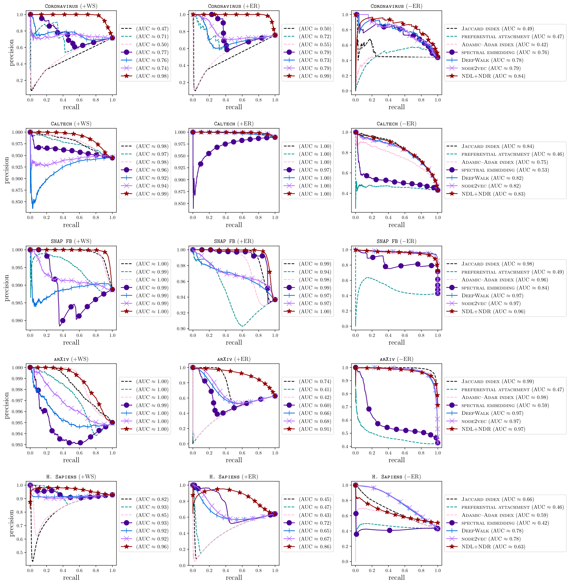


References
- [153] Jukka-Pekka Onnela et al. “Taxonomies of networks from community structure” In Physical Review E 86.3 APS, 2012, pp. 036104
- [154] Ankit. Khambhati, Ann. Sizemore, Richard. Betzel and Danielle. Bassett “Modeling and interpreting mesoscale network dynamics” In NeuroImage 180 Elsevier, 2018, pp. 337–349
- [155] Hanbaek Lyu, Deanna Needell and Laura Balzano “Online matrix factorization for Markovian data and applications to network dictionary learning” In Journal of Machine Learning Research 21, 2020, pp. 1–49
- [156] Hanbaek Lyu, Facundo Memoli and David Sivakoff “Sampling random graph homomorphisms and applications to network data analysis” In Journal of Machine Learning Research 24, 2023, pp. 1–79
- [157] Daniel. Lee and H. Seung “Learning the parts of objects by non-negative matrix factorization” In Nature 401.6755 Nature Publishing Group, 1999, pp. 788–791
- [158] Mark E.. Newman “Networks” Oxford, UK: Oxford University Press, 2018
- [159] Alice. Schwarze and Mason. Porter “Motifs for processes on networks” In SIAM Journal on Applied Dynamical Systems 20.4, 2021, pp. 2516–2557
- [160] Ron Milo et al. “Network motifs: Simple building blocks of complex networks” In Science 298.5594 American Association for the Advancement of Science, 2002, pp. 824–827
- [161] Gavin. Conant and Andreas Wagner “Convergent evolution of gene circuits” In Nature Genetics 34.3 Nature Publishing Group, 2003, pp. 264–266
- [162] Jason M.. Rip, Kevin. McCann, Denis. Lynn and Sonia Fawcett “An experimental test of a fundamental food web motif” In Proceedings of the Royal Society B: Biological Sciences 277.1688 The Royal Society, 2010, pp. 1743–1749
- [163] Olaf Sporns, Rolf K\"otter and Karl. Friston “Motifs in brain networks” In PLoS Biology 2.11 Public Library of Science San Francisco, USA, 2004, pp. e369
- [164] Konstantin Ristl, Sebastian. Plitzko and Barbara Drossel “Complex response of a food-web module to symmetric and asymmetric migration between several patches” In Journal of Theoretical Biology 354 Elsevier, 2014, pp. 54–59
- [165] Uri Alon “Network motifs: Theory and experimental approaches” In Nature Reviews Genetics 8.6 Nature Publishing Group, 2007, pp. 450–461
- [166] Xu Hong-lin, Yan Han-bing, Gao Cui-fang and Zhu Ping “Social network analysis based on network motifs” In Journal of Applied Mathematics 2014 Hindawi, 2014, pp. 874708
- [167] Krzysztof Juszczyszyn, Przemyslaw Kazienko and Bogdan Gabrys “Temporal changes in local topology of an email-based social network” In Computing and Informatics 28.6, 2009, pp. 763–779
- [168] Takaaki Ohnishi, Hideki Takayasu and Misako Takayasu “Network motifs in an inter-firm network” In Journal of Economic Interaction and Coordination 5.2 Springer, 2010, pp. 171–180
- [169] Frank. Takes, Walter. Kosters, Boyd Witte and Eelke. Heemskerk “Multiplex network motifs as building blocks of corporate networks” In Applied Network Science 3.1 Springer, 2018, pp. 39
- [170] Bryan Perozzi, Rami Al-Rfou and Steven Skiena “DeepWalk: Online learning of social representations” In Proceedings of the 20th ACM SIGKDD International Conference on Knowledge Discovery and Data Mining, 2014, pp. 701–710
- [171] Aditya Grover and Jure Leskovec “node2vec: Scalable feature learning for networks” In Proceedings of the 22nd ACM SIGKDD International Conference on Knowledge Discovery and Data Mining, 2016, pp. 855–864
- [172] C. Seshadhri, Aneesh Sharma, Andrew Stolman and Ashish Goel “The impossibility of low-rank representations for triangle-rich complex networks” In Proceedings of the National Academy of Sciences of the United States of America 117.11 National Academy of Sciences, 2020, pp. 5631–5637
- [173] Leman Akoglu, Hanghang Tong and Danai Koutra “Graph based anomaly detection and description: A survey” In Data Mining and Knowledge Discovery 29 Springer, 2015, pp. 626–688
- [174] Caleb. Noble and Diane. Cook “Graph-based anomaly detection” In Proceedings of the Ninth ACM SIGKDD International Conference on Knowledge Discovery and Data Mining, 2003, pp. 631–636
- [175] Benjamin. Miller, Michelle. Beard, Patrick. Wolfe and Nadya. Bliss “A spectral framework for anomalous subgraph detection” In IEEE Transactions on Signal Processing 63.16 IEEE, 2015, pp. 4191–4206
- [176] Xiaoxiao Ma et al. “A comprehensive survey on graph anomaly detection with deep learning” In IEEE Transactions on Knowledge and Data Engineering IEEE, 2021
- [177] Michael Elad and Michal Aharon “Image denoising via sparse and redundant representations over learned dictionaries” In IEEE Transactions on Image Processing 15.12 IEEE, 2006, pp. 3736–3745
- [178] Julien Mairal, Michael Elad and Guillermo Sapiro “Sparse representation for color image restoration” In IEEE Transactions on Image Processing 17.1 IEEE, 2007, pp. 53–69
- [179] Gabriel Peyr\’e “Sparse modeling of textures” In Journal of Mathematical Imaging and Vision 34.1 Springer, 2009, pp. 17–31
- [180] Veronica Red, Eric. Kelsic, Peter. Mucha and Mason. Porter “Comparing community structure to characteristics in online collegiate social networks” In SIAM Review 53, 2011, pp. 526–543
- [181] Amanda. Traud, Peter. Mucha and Mason. Porter “Social structure of Facebook networks” In Physica A 391.16 Elsevier, 2012, pp. 4165–4180
- [182] Mason. Porter, Jukka-Pekka Onnela and Peter. Mucha “Communities in networks” In Notices of the American Mathematical Society 56.9, 2009, pp. 1082–1097, 1164–1166
- [183] Santo Fortunato and Darko Hric “Community detection in networks: A user guide” In Physics Reports 659 Elsevier, 2016, pp. 1–44
- [184] Rose Oughtred et al. “The BioGRID interaction database: 2019 update” In Nucleic Acids Research 47.D1 Oxford University Press, 2019, pp. D529–D541
- [185] theBiogrid.org “Coronavirus PPI network” Retrieved from https://wiki.thebiogrid.org/doku.php/covid (downloaded 24 July 2020, Ver. 3.5.187.tab3), 2020
- [186] David. Gordon et al. “A SARS-CoV-2 protein interaction map reveals targets for drug repurposing” In Nature 583 Nature Publishing Group, 2020, pp. 1–13
- [187] Jure Leskovec and Julian. McAuley “Learning to discover social circles in ego networks” In Proceedings of the 25th International Conference on Neural Information Processing Systems — Volume 1, 2012, pp. 539–547
- [188] Jure Leskovec and Andrej Krevl “SNAP Datasets: Stanford Large Network Dataset Collection” Available at http://snap.stanford.edu/data, 2020
- [189] Paul Erdos and Alfr\’ed R\’enyi “On random graphs. I” In Publicationes Mathematicae 6.18, 1959, pp. 290–297
- [190] Duncan. Watts and Steven. Strogatz “Collective dynamics of ‘small-world’ networks” In Nature 393.6684 Nature Publishing Group, 1998, pp. 440–442
- [191] Albert-L\’aszl\’o Barab\’asi and R\’eka Albert “Emergence of scaling in random networks” In Science 286.5439 American Association for the Advancement of Science, 1999, pp. 509–512
- [192] Paul. Holland, Kathryn Laskey and Samuel Leinhardt “Stochastic blockmodels: First steps” In Social Networks 5.2 Elsevier, 1983, pp. 109–137
- [193] William. Rand “Objective criteria for the evaluation of clustering methods” In Journal of the American Statistical Association 66.336 Taylor & Francis Group, 1971, pp. 846–850
- [194] Lucas G.. Jeub et al. “Think locally, act locally: Detection of small, medium-sized, and large large networks” In Physical Review E 91.1 American Physical Society, 2015, pp. 012821
- [195] Rajul Parikh et al. “Understanding and using sensitivity, specificity and predictive values” In Indian Journal of Ophthalmology 56.1 Wolters Kluwer–Medknow Publications, 2008, pp. 45
- [196] Fernanda. Correia, Edgar. Coelho, Jos\’e. Oliveira and Joel. Arrais “Handling noise in protein interaction networks” In BioMed Research International 2019 Hindawi, 2019, pp. 8984248
- [197] Tao Zhou “Progresses and challenges in link prediction” In iScience 24.11, 2021, pp. 103217
- [198] David Liben-Nowell and Jon Kleinberg “The link-prediction problem for social networks” In Journal of the American Society for Information Science and Technology 58.7 Wiley Online Library, 2007, pp. 1019–1031
- [199] Aditya Menon and Charles Elkan “Link prediction via matrix factorization” In Machine Learning and Knowledge Discovery in Databases Heidelberg, Germany: Springer-Verlag, 2011, pp. 437–452
- [200] Istv\’an. Kov\’acs et al. “Network-based prediction of protein interactions” In Nature Communications 10.1 Nature Publishing Group, 2019, pp. 1240
- [201] Roger Guimer\‘a “One model to rule them all in network science?” In Proceedings of the National Academy of Sciences of the United States of America 117.41 National Acad Sciences, 2020, pp. 25195–25197
- [202] Mohammad Hasan and Mohammed. Zaki “A survey of link prediction in social networks” In Social Network Data Analytics Springer, 2011, pp. 243–275
- [203] Ivan Markovsky and Konstantin Usevich “Low Rank Approximation” Heidelberg, Germany: Springer-Verlag, 2012
- [204] Ashwin Paranjape, Austin Benson and Jure Leskovec “Motifs in temporal networks” In Proceedings of the Tenth ACM International Conference on Web Search and Data Mining, 2017, pp. 601–610
- [205] Federico Battiston, Vincenzo Nicosia, Mario Chavez and Vito Latora “Multilayer motif analysis of brain networks” In Chaos: An Interdisciplinary Journal of Nonlinear Science 27.4 AIP Publishing LLC, 2017, pp. 047404
- [206] Daniel. Lee and H. Seung “Algorithms for non-negative matrix factorization” In Proceedings of the 13th International Conference on Neural Information Processing Systems, 2001, pp. 556–562
- [207] Julien Mairal, Francis Bach, Jean Ponce and Guillermo Sapiro “Online learning for matrix factorization and sparse coding” In Journal of Machine Learning Research 11, 2010, pp. 19–60
- [208] Julien Mairal, Michael Elad and Guillermo Sapiro “Sparse learned representations for image restoration” In Proceedings of the 4th World Conference of the International Association for Statistical Computing, 2008, pp. 118 IASC
- [209] Julien Mairal et al. “Non-local sparse models for image restoration” In 2009 IEEE 12th International Conference on Computer Vision, 2009, pp. 2272–2279 IEEE
- [210] theBiogrid.org “Homo sapiens PPI network” Retrieved from https://wiki.thebiogrid.org/doku.php/covid (downloaded 24 July 2020, Ver. 3.5.180.tab2), 2020
- [211] L\’aszl\’o Lov\’asz “Large Networks and Graph Limits” 60, Colloquium Publications Providence, RI, USA: American Mathematical Society, 2012, pp. 475
- [212] Marco Bressan “Efficient and near-optimal algorithms for sampling connected subgraphs” In Proceedings of the 53rd Annual ACM SIGACT Symposium on Theory of Computing, STOC 2021 Virtual, Italy: Association for Computing Machinery, 2021, pp. 1132–1143
- [213] Nadav Kashtan, Shalev Itzkovitz, Ron Milo and Uri Alon “Efficient sampling algorithm for estimating subgraph concentrations and detecting network motifs” In Bioinformatics 20.11 Oxford University Press, 2004, pp. 1746–1758
- [214] Sebastian Wernicke “Efficient detection of network motifs” In IEEE/ACM Transactions on Computational Biology and Bioinformatics 3.4 IEEE, 2006, pp. 347–359
- [215] Jure Leskovec and Christos Faloutsos “Sampling from large graphs” In Proceedings of the 12th ACM SIGKDD International Conference on Knowledge Discovery and Data Mining, 2006, pp. 631–636
- [216] Paul Glasserman “Monte Carlo Methods in Financial Engineering” Heidelberg, Germany: Springer-Verlag, 2004
- [217] David. Levin and Yuval Peres “Markov Chains and Mixing Times” Providence, RI, USA: American Mathematical Society, 2017
- [218] Bradley Efron, Trevor Hastie, Iain Johnstone and Robert Tibshirani “Least angle regression” In The Annals of Statistics 32.2 Institute of Mathematical Statistics, 2004, pp. 407–499
- [219] Robert Tibshirani “Regression shrinkage and selection via the lasso” In Journal of the Royal Statistical Society: Series B (Methodological) 58.1 Wiley Online Library, 1996, pp. 267–288
- [220] Honglak Lee, Alexis Battle, Rajat Raina and Andrew. Ng “Efficient sparse coding algorithms” In Advances in Neural Information Processing Systems, 2007, pp. 801–808
- [221] Roger. Horn and Charles. Johnson “Matrix Analysis” Cambridge, UK: Cambridge University Press, 2012
- [222] Vincent. Blondel, Jean-Loup Guillaume, Renaud Lambiotte and Etienne Lefebvre “Fast unfolding of communities in large networks” In Journal of Statistical Mechanics: Theory and Experiment 2008.10 IOP Publishing, 2008, pp. P10008
- [223] George. Brown and Alexander. Mood “On median tests for linear hypotheses” In Proceedings of the Second Berkeley Symposium on Mathematical Statistics and Probability 2, 1951, pp. 159–166 University of California Press
- [224] Lei Tang and Huan Liu “Leveraging social media networks for classification” In Data Mining and Knowledge Discovery 23.3 Springer, 2011, pp. 447–478
- [225] Tomas Mikolov et al. “Distributed representations of words and phrases and their compositionality” In Proceedings of the 26th International Conference on Neural Information Processing Systems — Volume 2, 2013, pp. 3111–3119
- [226] Richard. Durrett “Probability: Theory and Examples”, Cambridge Series in Statistical and Probabilistic Mathematics Cambridge, UK: Cambridge University Press, 2010, pp. 428
- [227] Sean. Meyn and Richard. Tweedie “Markov Chains and Stochastic Stability” Heidelberg, Germany: Springer-Verlag, 2012
- [228] Julien Mairal “Stochastic majorization–minimization algorithms for large-scale optimization” In Proceedings of the 26th International Conference on Neural Information Processing Systems — Volume 2, 2013, pp. 2283–2291