Precise transit and radial-velocity characterization of a resonant pair: a warm Jupiter TOI-216c and eccentric warm Neptune TOI-216bJournal: AJ mpfit (Markwardt 2009), TAP(Gazak et al. 2012), Tapir (Jensen 2013), TESS pipeline (Jenkins et al. 2016; Twicken et al. 2018; Li et al. 2019), AstroImageJ (Collins et al. 2017), exoplanet (Foreman-Mackey et al. 2019), astropy (Astropy Collaboration et al. 2013; Astropy Collaboration et al. 2018), celerite (Foreman-Mackey et al. 2017; Foreman-Mackey 2018), starry (Luger et al. 2019), pymc3 (Salvatier et al. 2016), theano (Theano Development Team 2016), ceres (Brahm et al. 2017), PyTTV, PyTransit (Parviainen 2015), emcee (Foreman-Mackey et al. 2013), eleanor (Feinstein et al. 2019)
Abstract
TOI-216 hosts a pair of warm, large exoplanets discovered by the TESS Mission. These planets were found to be in or near the 2:1 resonance, and both of them exhibit transit timing variations (TTV). Precise characterization of the planets’ masses and radii, orbital properties, and resonant behavior can test theories for the origins of planets orbiting close to their stars. Previous characterization of the system using the first six sectors of TESS data suffered from a degeneracy between planet mass and orbital eccentricity. Radial velocity measurements using HARPS, FEROS, and PFS break that degeneracy, and an expanded TTV baseline from TESS and an ongoing ground-based transit observing campaign increase the precision of the mass and eccentricity measurements. We determine that TOI-216c is a warm Jupiter, TOI-216b is an eccentric warm Neptune, and that they librate in the 2:1 resonance with a moderate libration amplitude of degrees; small but significant free eccentricity of for TOI-216b; and small but significant mutual inclination of 1.2–3.9∘ (95% confidence interval). The libration amplitude, free eccentricity, and mutual inclination imply a disturbance of TOI-216b before or after resonance capture, perhaps by an undetected third planet.
I Introduction
Warm Jupiters – defined here as giant planets with 10–100 day orbital periods – in systems with other nearby planets are an important population for the investigation of giant planets close to their stars. High eccentricity tidal migration – a strong contender for the origins of many close-in giant planets (see Dawson & Johnson 2018 for a review) is unlikely to have been at work in these systems (e.g., Mustill et al. 2015). Disk migration has been a persistently proposed explanation (e.g., Lee & Peale 2002) – particularly for systems in or near mean motion resonance – but recent studies have argued that in situ formation may be more consistent with these planets’ observed properties (e.g., Huang et al. 2016; Frelikh et al. 2019; Anderson et al. 2020) and could possibly be consistent with resonant configurations (e.g., Dong & Dawson 2016; MacDonald & Dawson 2018; Choksi & Chiang 2020). Precise characterization of the orbital properties and resonant behavior of individual systems can test origins scenarios, complementary to population studies.
One warm Jupiter system potentially amenable to such detailed characterization is TOI-216, which hosts a pair of warm, large exoplanets discovered by the TESS Mission (Dawson et al. 2019; Kipping et al. 2019). Their masses and orbits were characterized using transit timing variations (TTVs). However, previously the TESS TTV dataset was not sufficiently precise to break the degeneracy between mass and eccentricity that arises when we can measure the near-resonant TTV signal but not the chopping TTV signal (e.g., Lithwick & Naoz 2011; Deck & Agol 2015). Different priors on mass and eccentricity led to two qualitatively different solutions for the system (Dawson et al. 2019): a Jupiter-mass planet accompanied by a Saturn-mass planet librating in orbital resonance, and a puffy sub-Saturn-mass planet and puffy Neptune-mass planet near but not in orbital resonance. The solutions also differed in the planets’ free eccentricity, the eccentricity not associated with the proximity to resonance. Since any origins scenario under consideration needs to be able to account for the planets’ masses, free eccentricities, and resonant behavior, detailed characterization of these properties with a more extended dataset is warranted.
Since our previous study (Dawson et al. 2019), seven more TESS transits of planet b, three more TESS transits of planet c, a ground-based transit of planet b, and five more ground-based transits of planet c have been observed, including recent ground-based transit observations that significantly extend the baseline for measuring transit timing variations beyond the observations conducted during the first year of the TESS primary mission. Furthermore, we have been conducting a ground-based radial-velocity campaign using HARPS, FEROS, and PFS. Radial-velocity measurements serve to break the mass-eccentricity degeneracy.
Here we combine TESS light curves, ground-based light curves, and ground-based radial velocities to precisely characterize TOI-216b and c. In Section II, we describe our analysis of the TESS data and the observation and analysis of ground-based light curves. We identify a weak stellar activity periodicity in the TESS data that also shows up in the radial velocities. In Section III, we present radial velocity measurements from HARPS, FEROS, and PFS and show that they immediately confirm the higher mass, lower eccentricity solution. We investigate additional weak periodicities in the radial-velocities and argue that they are caused by stellar activity. We jointly fit the transit timing variations and radial velocities in Section IV and determine that the planet pair is librating in resonance, that the inner planet has a significant free eccentricity, and that planets have a small but significant mutual inclination. We present our conclusions – including implications for the system’s origins – in Section V.
II Light Curve Analysis
This paper is based on data from TESS Sectors 1–13 (2018 July 25 – 2019 July 17) and Sectors 27–30 (2020 July 4 – 2020 October 21), during which TOI-216 was observed with CCD 1 on Camera 4, and from ground-based observatories. We use the publicly available 2-min cadence TESS data, which is processed with the Science Processing Operations Center pipeline (Jenkins et al. 2016). We download the publicly available data from the Mikulski Archive for Space Telescopes (MAST). The pipeline, a descendant of the Kepler mission pipeline based at the NASA Ames Research Center (Jenkins et al. 2002; Jenkins et al. 2010), analyzes target pixel postage stamps that are obtained for pre-selected target stars.
We use the resources of the TESS Follow-up Observing Program (TFOP) Working Group (WG) Sub Group 1 (SG1)11 1 https://tess.mit.edu/followup/ to collect seeing-limited time-series photometric follow-up of TOI-216. All photometric time series are publicly available on the Exoplanet Follow-up Observing Program for TESS (ExoFOP-TESS) website22 2 https://exofop.ipac.caltech.edu/tess/. Light curves observed on or before February 24, 2019 are described in Dawson et al. 2019. Our new time-series follow-up observations are listed in Table 1. We used the TESS Transit Finder, which is a customized version of the Tapir software package (Jensen 2013), to schedule our transit observations. Unless otherwise noted, the photometric data were extracted using the AstroImageJ (AIJ) software package (Collins et al. 2017). The facilities used to collect the new TOI-216 observations published here are Las Cumbres Observatory Global Telescope (LCOGT) network (Brown et al. 2013), Hazelwood Observatory (Churchill, Vic, Australia), El Sauce Observatory (Coquimbo Province, Chile), and the Antarctic Search for Transiting ExoPlanets (ASTEP) observatory (Concordia Station, Antarctica). All LCOGT 1 m telescopes are equipped with the Sinistro camera, with a 4k4k pixel Fairchild back illuminated CCD and a FOV. The LCOGT images were calibrated using the standard LCOGT BANZAI pipeline (McCully et al. 2018). Hazelwood is a private observatory with an f/8 Planewave Instruments CDK12 0.32 m telescope and an SBIG STT3200 2.2k1.5k CCD, giving a field of view. El Sauce is a private observatory which hosts a number of telescopes; the observations reported here were carried out with a Planewave Instruments CDK14 0.36 m telescope and an SBIG STT-1603-3 1536k1024k CCD, giving a field of view. ASTEP is a 0.4 m telescope with an FLI Proline 16801E 4k4k CCD, giving a field of view. The ASTEP photometric data were extracted using a custom IDL-based pipeline.
| TOI-216 | Date | Telescope${\dagger}$${\dagger}$Telescopes:
LCOGT-CTIO-1.0: Las Cumbres Observatory - Cerro Tololo Inter-American Observatory (1.0 m) LCOGT-SAAO-1.0: Las Cumbres Observatory - South African Astronomical Observatory (1.0 m) LCOGT-SSO-1.0: Las Cumbres Observatory - Siding Spring Observatory (1.0 m) Hazelwood-0.3: Stockdale Private Observatory - Victoria, Australia (0.32 m) El Sauce-0.36: El Sauce Observatory - Coquimbo Province, Chile (0.36 m) ASTEP-0.4: Antarctic Search for Transiting ExoPlanets - Concordia Station, Antarctica (0.4 m) |
Filter | ExpT | Exp | Dur. | Transit | Ap. Radius | FWHM |
| (UTC) | (sec) | (N) | (min) | Coverage | (arcsec) | (arcsec) | |||
| b | 2019-10-30 | LCOGT-CTIO-1.0 | I | 40 | 220 | 241 | Full | 5.8 | 2.4 |
| 2020-05-23 | ASTEP-0.4 | Rc | 120 | 376 | 924 | Full | 10.2 | 5.3 | |
| c | 2018-12-16 | LCOGT-SAAO-1.0 | i′ | 90 | 331 | 450 | Full | 5.8 | 2.1 |
| 2019-01-20 | Hazelwood-0.3 | g′ | 240 | 101 | 449 | Egress+70 | 5.5 | 3.2 | |
| 2019-02-24 | El Sauce-0.36 | Rc | 30 | 514 | 303 | Egress+90 | 5.9 | 3.4 | |
| 2019-06-07 | ASTEP-0.4 | Rc | 120 | 549 | 1440 | Full | 12.0 | 5.0 | |
| 2019-11-27 | Hazelwood-0.3 | Rc | 60 | 114 | 255 | Egress+60 | 5.5 | 3.1 | |
| 2019-12-31 | LCOGT-SAAO-1.0 | Ic | 40 | 316 | 345 | Ingress+90 | 4.7 | 2.0 | |
| 2020-02-24 | Hazelwood-0.3 | Rc | 120 | 161 | 380 | Egress+60 | 5.5 | 3.1 | |
| 2020-03-09 | LCOGT-CTIO-1.0 | I | 40 | 146 | 176 | Egress+30 | 8.2 | 2.6 | |
| 2020-06-21 | ASTEP-0.4 | Rc | 120 | 272 | 656 | Full | 11.0 | 5.0 |
We fit the transit light curves (Fig. 1) using the TAP software package (Gazak et al. 2012), which implements Markov Chain Monte Carlo using the Mandel & Agol 2002 transit model and the Carter & Winn 2009 wavelet likelihood function, with the modifications described in Dawson et al. 2014. The results are summarized in Table 2. For TESS light curves, we use the presearch data conditioned (PDC) flux, which is corrected for systematic (e.g., instrumental) trends using cotrending basis vectors (Smith et al. 2012; Stumpe et al. 2014). For all light curves, we use Carter & Winn 2009 wavelet likelihood function (which, for the red noise component, assumes noise with an amplitude that scales as frequency-1) with free parameters for the amplitude of the red and white noise and a linear trend fit simultaneously to each transit light curve segment with other transit parameters. For the ground-based observations, we fit a linear trend to airmass instead of time. We assign each instrument and filter (TESS, Hazelwood g’ and Rc, LCOGT i’ and I, El Sauce Rc, and ASTEP Rc) its own set of limb darkening parameters because of the different wavebands. We use one set of noise parameters for all the TESS light curves and an additional set for each ground-based light curve. We adopt uniform priors on the planet-to-star radius ratio (), the impact parameter (which can be either negative or positive; we report ), the mid transit time, the limb darkening coefficients and (Kipping 2013a), and the slope and intercept of each transit segment’s linear trend. For the grazing transits of the inner planet, we impose a uniform prior on from 0 to 0.17, with the upper limit corresponding to a planet radius of 0.13 solar radii (see Dawson et al. 2019 for details and justification). Despite a well-constrained transit depth (Table 2), the inner planet’s radius ratio is highly uncertain due to degeneracy between the radius ratio and impact parameter (see Fig. 3 of Dawson et al. 2019). We also impose a uniform prior on the log of the light curve stellar density . We use , the stellar density derived from the light curve assuming a circular orbit, to compute the Mandel & Agol 2002 model normalized separation of centers , assuming and a circular orbit:
| (1) |
where is the orbital period, the subscript denotes the Earth, and the subscript denotes the Sun. We will later combine the posteriors from the light curve and (from Dawson et al. 2019’s isochrone fit) to constrain the orbital eccentricity (Section IV.2). We perform an additional set of fits where we allow for a dilution factor for the TESS light curves and find the results to be indistinguishable. We measure a dilution factor of .


We also perform two additional fits to look for transit duration variations, following Dawson 2020. In the first fit, we allow the impact parameter to vary with the prior recommended by Dawson 2020. We find tentative evidence for the variation in the transit impact parameter for the inner planet, with an impact parameter change scale of 0.007. In the second fit, we allow (Eqn. 1) and to vary for each transit with a prior that corresponds to a uniform prior in transit duration (Dawson 2020). Again the inner planet exhibits tentative evidence for variation in its transit durations. We fit a line to the transit durations as a function of mid-transit time and determine a three-sigma confidence interval on the slope of -0.4 – 4 seconds/day for the inner planet and -1 – 0.4 seconds/day for the outer planet.
For comparison and to ensure that the results are not sensitive to the correlated noise treatment, we also fit the light curves using the exoplanet package (Foreman-Mackey et al. 2019), which uses Gaussian process regression. Each set of TESS light curves along with eight ground-based light curves is modeled with a light curve transit model built from starry (Luger et al. 2019) plus a Matern-3/2 Gaussian process kernel with a white noise term. Seven sets of limb-darkening parameters (Kipping 2013b) are used for observations conducted in seven different filters. We use a log-uniform prior on stellar densities (), log-normal prior on transit depths, uniform prior on the impact parameters, and uniform prior on mid-transit times. We infer posteriors for each parameter using this approach that are consistent within 1 sigma to our nominal fit above.
| Parameter | ValueaaAs a summary statistic we report the median and 68.3% confidence interval of the posterior distribution. | |
|---|---|---|
| TOI-216b | ||
| Planet-to-star radius ratio, | 0.10 | |
| Transit depth [ppm] | 4750 | |
| Planet radius, [] | 8 | |
| Light curve stellar densitybbEqn. 1, [] | 1.1 | |
| Impact parameter, | 0.98 | |
| Mid-transit times (daysc,dc,dfootnotemark: ) | 1325.328 | |
| 1342.430 | ||
| 1359.540 | ||
| 1376.631 | ||
| 1393.723 | ||
| 1427.879 | ||
| 1444.958 | ||
| 1462.031 | ||
| 1479.094 | ||
| 1496.155 | ||
| 1513.225 | ||
| 1547.338 | ||
| 1564.403 | ||
| 1598.529 | ||
| 1615.604 | ||
| 1632.679 | ||
| 1649.759 | ||
| 1666.851 | ||
| LCOGT | 1786.698 | |
| ASTEP | 1993.486 | |
| 2045.465 | ||
| 2062.800 | ||
| 2080.157 | ||
| 2097.511 | ||
| 2132.243 | ||
| Best fit linear ephemeris: | ||
| Period (days) | 17.16073 | |
| Epoch (days) | 1324.5911 | |
| TOI-216c | ||
| Planet-to-star radius ratio, | 0.1230 | |
| Transit depth [ppm] | 18310 | |
| Planet radius, [] | 10.1 | |
| Light curves stellar density, [] | 1.73 | |
| Impact parameter, | 0.14 | |
| Mid-transit times (daysc,dc,dfootnotemark: ) | 1331.2850 | |
| 1365.8244 | ||
| 1400.3686 | ||
| 1434.9227 | ||
| 1469.4773 | ||
| LCOGT | 1469.4781 | |
| Hazelwood | 1504.036 | |
| El Sauce | 1538.5938 | |
| 1538.5921 | ||
| 1607.7082 | ||
| 1642.2612 | ||
| ASTEP | 1642.2595 | |
| 1676.8085 | ||
| Hazelwood | 1814.939 | |
| LCOGT | 1849.4526 | |
| Hazelwood | 1883.955 | |
| LCOGT | 1918.4506 | |
| ASTEP | 2021.8887 | |
| 2056.3520 | ||
| 2090.8107 | ||
| 2125.2698 | ||
| Best fit linear ephemeris: | ||
| Period (days) | 34.525528 | |
| Epoch (days) | 1331.4110 |
We examine the light curve for evidence of stellar rotation. We do not see any significant periodicities in the SPOC 2 minute cadence data. To investigate further, we create a systematics-corrected long cadence light curve using eleanor (Feinstein et al. 2019) with a 15 x 15 target pixel file, background size of 100, and custom square aperture of 3x3 pixels centered on TOI-216. We follow eleanor’s recommendation for background subtraction: the 1D postcard background for sectors 1, 2, 4, 6, 7, 8, 11 and 13; the 1D target pixel file background for sectors 3 and 5; and the 2D target pixel file background for sectors 9 and 12. Then we mask out the transits and compute a discrete autocorrelation function (DCF; Eqn. 2 of Edelson & Krolik 1988), plotted in Fig. 2.
The peak at 6.5 day and valley at approximately half that value are consistent with a 6.5 day periodicity. This periodicity could represent the rotation period or a shorter harmonic. A rotation period of days would be most typical for a 0.78 star on the main sequence (e.g., McQuillan et al. 2014), so the periodicity could plausibly be an integer fraction of the rotation period (e.g., one half, one third). The stellar radius of 0.747 (Dawson et al. 2019) and km/s from the FEROS spectra correspond to a rotation period of days assuming an edge-on orientation. A rotation period of 26 days would be compatible with the measurement, or a shorter rotation period would indicate a spin-orbit misalignment. A periodicity of 13 days or 26 days is challenging to detect in the TESS light curve (e.g., Canto Martins et al. 2020). 13 days is close to TESS’s 13.7 day orbital period and thus susceptible to corrections for systematics. Both are a significant fraction of the sector (27 days) and subject to imprecision in stitching together different segments. Given the many bumps and wiggles in the DCF, we do not consider this lightcurve detection of a stellar rotation harmonic definitive.

| [ppm] | [ppm] | |||||||
|---|---|---|---|---|---|---|---|---|
| TESS | ||||||||
| 2 min | 3900 | 2475 | ||||||
| 20 s | 15000 | 5364 | ||||||
| LCOGT i’ | 1600 | 1060 | ||||||
| Hazelwood g’ | 4000 | 2450 | ||||||
| El Sauce | 3130 | |||||||
| Hazelwood Rc: | ||||||||
| Nov. 2019 | 9000 | 2100 | ||||||
| Feb. 2020 | 1920 | |||||||
| LCOGT I: | ||||||||
| Oct. 2019 | 1400 | 2360 | ||||||
| Dec. 2019 | 1200 | 1130 | ||||||
| Mar. 2020 | 1600 | 990 | ||||||
| ASTEP | ||||||||
| June 2019 | 13000 | 2100 | ||||||
| May 2020 | 3800 | 1270 | ||||||
| June 2020 | 11900 | 1360 |
III Radial velocity analysis
TOI-216 was monitored with three different high resolution echelle spectrographs over a time span of 16 months with the goal of obtaining precision radial velocities to further constrain the masses and orbital parameters of the giant planets present in the TOI-216 system. These observations were performed in the context of the Warm gIaNts with tEss (WINE) collaboration, which focuses on the systematic characterization of TESS transiting giant planets with orbital periods longer than 10 days (Brahm et al. 2019; Jordán et al. 2020, e.g.,). All radial velocity measurements of TOI-216 are presented in Table 5.
We obtained 27 spectra with the Fibre-fed, Extended Range, Échelle Spectrograph (Kaufer et al. 1999, FEROS,) between November of 2018 and March of 2019. FEROS is mounted on the MPG 2.2 m telescope at the ESO La Silla Observatory, and has a resolving power of R 48 000. Observations were performed with the simultaneous calibration mode for tracing radial velocity variations produced by environmental changes in the instrument enclosure. The adopted exposure time of 1200 seconds yielded spectra with signal-to-noise ratios in the range from 40 to 75. FEROS spectra were processed from raw data with the ceres pipeline (Brahm et al. 2017), which delivers precision radial velocities and line bisector span measurements via cross-correlation with a binary mask resembling the spectral properties of a G2-type star. The radial velocity uncertainties for the FEROS observations of TOI-216 range between 7 and 15 m s-1. We remove two outliers from the FEROS radial-velocity time series at 1503.75 and 1521.57 days. All subsequent results do not include these outliers. We have checked that no results except the inferred jitter for the FEROS dataset are sensitive to whether or not the outliers are included.
We observed TOI-216 on 15 different epochs between December of 2018 and October of 2019 with the High Accuracy Radial velocity Planet Searcher (Mayor et al. 2003, HARPS) mounted on the ESO 3.6 m telescope at the ESO La Silla Observatory, in Chile. We adopted an exposure time of 1800 seconds for these observations using the high radial velocity accuracy mode (HAM, R 115 000), which produced spectra with signal-to-noise ratios of 40 per resolution element. As in the case of FEROS, HARPS data for TOI-216 was processed with the ceres pipeline, delivering radial velocity measurements with typical errors of 5 m s-1.
TOI-216 was also monitored with the Planet Finder Spectrograph (Crane et al. 2006; Crane et al. 2008; Crane et al. 2010, PFS;) mounted on the 6.5 m Magellan II Clay Telescope at Las Campanas Observatory (LCO), in Chile. These spectra were obtained on 18 different nights, between December of 2018 and March of 2020, using the 0.32.5 slit, which delivers a resolving power of = 130 000. Due to its moderate faintness, TOI-216 was observed with the 33 binning mode to minimize read-out noise, and an exposure time of 1200 seconds was adopted to reach a radial velocity precision of 2 m s-1. An iodine cell was used in these observations as a reference for the wavelength calibration. The PFS data were processed with a custom IDL pipeline (Butler et al. 1996). Three consecutive 1200 second iodine-free exposures of TOI-216 were obtained to construct a stellar spectral template for disentangling the iodine spectra from the stellar one for computing the radial velocities.
It is immediately evident that the radial velocities show good agreement with Dawson et al. 2019’s higher mass solution, which was fit to the earlier, transit time only dataset (Fig. 3), and with Kipping et al. 2019’s solution based on transit times from the first six sectors. The bottom panel of Fig. 3 shows the RVs phased to the outer planet’s orbital period. We compute a generalised Lomb-Scargle periodogram (Cumming et al. 1999; Zechmeister & Kürster 2009) in Fig. 4 and 5. The x-axis is frequency in cycles per day. The y-axis is the square root of the power, where we define power as
| (2) |
where is the reported uncertainty (Table 5) and is the radial-velocity (Table 5) with the error weighted mean for each of the three datasets (PFS, HARPS, and FEROS) subtracted. The sinusoidal function is
| (3) |
where and are computed following Zechmeister & Kürster 2009, is each of the three datasets, is the time of the first observed radial velocity, and
| (4) |
We see a peak in the periodogram at planet c’s orbital period (Fig. 4, left panel). The noise-free c model (overplotted, dashed; a Keplerian signal computed using the parameters of planet c from Table 4 sampled at the observed times in Table 5) shows that many of the other peaks seen in the three periodograms are aliases of planet c’s orbital period ( i.e., they caused by the observational time sampling of the planet’s signal). Planet b’s signal is below the noise level (Fig. 3, bottom right panel; Figure 4, right panels). In the PFS dataset, including planet b improves the chi-squared from 403 to 328 (for 18 datapoints and five additional parameters); for the HARPS and FEROS datasets, there is no improvement in chi-squared. Given that planet b is barely detected, we cannot rule out other planets in the system with smaller orbital radial velocity amplitudes.
Systems containing an outer planet in or near a 2:1 mean motion resonance with a less massive inner planet can be mistaken for a single eccentric planet, because the first eccentricity harmonic appears at half the planet’s orbital period (e.g., Anglada-Escudé et al. 2010; Kürster et al. 2015). In the case of the system TOI-216, the lack of detection of TOI-216b is not due to this phenomenon because solution we subtract off for planet c has near 0 eccentricity. However, without prior knowledge that the system contains a resonant pair, if we only had the radial-velocity datasets and the datasets were less noisy (or had more data points), we might be sensitive to planet b’s signal but mistakenly interpret it as planet c’s eccentricity.


The residuals of the two-planet fit (and one-planet fit) show evidence of a signal that we attribute to stellar activity. We examined the periodograms of the residuals of each of three datasets; the bisectors for the HARPS and FEROS datasets; and H alpha for the FEROS dataset, computed with the ceres pipeline, following Boisse et al. 2009. Periodograms of the PFS residuals and FEROS H alpha are shown in Figure 5. There are no strong peaks in any of the residual or activity indicator periodograms. Some residuals datasets exhibit (weak) peaks near the 6.5 day periodicity (HARPS residuals and bisectors; FEROS residuals) identified in the light curve (Section II), or a multiple of 6.5 days (PFS; FEROS bisectors and H alpha). In Fig. 6, we plot the residuals of the two-planet fit with best-fit sinusoids for 6.5, 13, and 26 day periodicities for each dataset. Comparing the three datasets, best-fit sinusoids are out of phase with each other. The similarity of the periodicities to those seen in the light curve, the appearance of the 6.5 day periodicity in the HARPS bisectors, the 6.5 and 26 day periodicities in the FEROS H alpha, and the 13 day and 6.5 day periodicities in the FEROS bisectors, and the difference in phase among datasets suggest the weak periodicities do not arise from additional planets. They are possibly caused by stellar variability.


IV Joint fit and orbital architecture
Here we jointly fit the transit light curves (Section II) and radial-velocity measurements (Section III) to precisely measure the orbital parameters and masses of both planets. In Section IV.1, we describe our analysis of the transit timing measurements. In Section IV.2, we jointly fit the transit and radial-velocity measurements.
IV.1 Transit timing variation analysis
TOI-216b and c exhibit transit timing variations – plotted in Fig. 7 – due to the near-resonant effect (e.g., Agol et al. 2005; Lithwick et al. 2012). We have not yet observed a full super-period (which depends on the planets’ proximity to the 2:1 resonance). The amplitude depends on the perturbing planet’s mass and the free eccentricity of the transiting and perturbing planets. We previously found a significant free eccentricity, with the exact value and partition between planets degenerate with planet mass (Dawson et al. 2019).

We fit the transit times using our N-body integrator TTV model (Dawson et al. 2014). Our model contains five parameters for each planet: the mass , orbital period , mean longitude , eccentricity , and argument of periapse . All orbital elements are osculating orbital elements at the epoch 1325.3279 days. For each planet, we fix the impact parameter to the value in Table 2 and set the longitude of ascending node on the sky to . We use the conventional coordinate system where the plane is the sky plane and the axis points toward the observer. We will explore other possibilities for and in Section IV.2.
We begin by fitting the transit times only. To explore the degeneracy between mass and eccentricity, we use the Levenberg-Marquardt alogrithm implemented in IDL mpfit (Markwardt 2009) to minimize the on a grid of . We first use a dataset consisting of all the ground-based data and the TESS Year 1 data. We contour the total for thirty-four transit times and ten free parameters, i.e., twenty-four degrees of freedom in Fig. 8. Even with the additional transits since Dawson et al. 2019, the fits still suffer from a degeneracy between mass and eccentricity, though the relationship is much tighter. We integrate a random sample of 100 solutions with and find that they all librate in the 2:1 resonance with the resonant angle involving the longitude of periapse of the inner planet. Next we add TESS Year 3 transits from the TESS Extended Mission, which became available while this manuscript was under review. This very extended baseline for the TTVs substantially reduces the degeneracy between mass and eccentricity. We also contour the total for these forty-three transit times and ten free parameters, i.e., thirty-three degrees of freedom in Fig. 8.
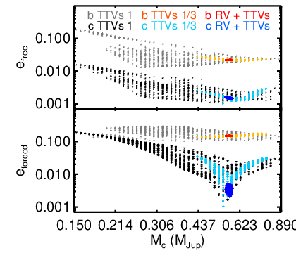
A resonant or near-resonant planet’s total eccentricity is the vector sum of its free and forced eccentricity. The forced eccentricity vector is dictated by the resonant dynamics, and the free eccentricity vector oscillates about the tip of the forced vector. Dissipation (e.g., eccentricity damping from the disk) tends to damp the free eccentricity, and other perturbations (e.g., from a third planet) can excite it. We estimate the eccentricity components from simulations as ) and ). The transit times continue to provide evidence for a moderate free eccentricity (Fig. 9), but pinning down the outer planet’s mass with a joint radial-velocity fit will allow for a tighter constraint.

IV.2 Joint transit and radial velocity fit
We perform a joint N-body fit to the transit times and radial velocities, imposing two additional constraints. One constraint is the transit exclusion intervals reported in Dawson et al. 2019. The other is the light curve joint posterior of stellar density vs. impact parameter (Table 2; Eqn. 1) combined with the posterior from Dawson et al. 2019. Following Dawson & Johnson 2012, we convert the vs. to a vs. posterior according to . We use the vs. posterior to add a term to the likelihood based on and using . We compute the sky-plane inclination for the dynamical model from according to .
Following Dawson et al. 2014, we derive posteriors for the parameters using Markov Chain Monte Carlo with the Metropolis-Hastings algorithm. Instead of including the orbital period and mean longitude at epoch 1325.3279 days as parameters in the MCMC, we optimize them at each jump (i.e., each MCMC step) using the Levenberg-Marquardt algorithm (i.e., optimizing the dynamical model). We also optimize the radial velocity offset for each instrument at each jump. We fit for a radial velocity jitter term for each of the three instruments; even though we identified possible periodicities in Fig. 5, none are strong enough to justify to explicitly modeling (e.g., with false alarm probabilities of 0.2, 0.002, and 0.02 for the highest peak in the periodogram for PFS, FEROS, and HARPS respectively; Cumming 2004). We visually inspect each parameter for convergence. We know there is a mutual inclination perpendicular to the sky plane because the inner planet exhibits grazing transits and the outer planet does not, To also allow for a mutual inclination parallel to the sky plane, we fit for , the difference in longitude of ascending node.
Following Dawson et al. 2019, we perform two fits with different priors to assess the sensitivity to these priors. The first solution (Table 4) imposes uniform priors on eccentricities and log uniform priors on mass (i.e., priors that are uniform in log space). The second imposes uniform priors on mass and log-uniform priors on eccentricity. All other fitted parameters (orbital period, mean longitude, argument of periapse, radial velocity jitters, difference in longitude of ascending node) have uniform priors. With the dataset in Dawson et al. 2019, the results were very sensitive to the priors; with the new dataset that includes radial-velocities and an expanded TTV baseline, the results with different priors are nearly indistinguishable. In both cases, we impose the three-sigma limits on change in transit duration derived in Section II. We measure a small but significant mutual inclination of 1.2–3.9∘ (95% confidence interval).
| Parameter | ValueaaAs a summary statistic we report the median and 68.3% confidence interval of the posterior distribution. An example fit with high precision suitable for numerical integration is given in Table 6. | |
|---|---|---|
| bbStellar parameters fixed to the values reported by Dawson et al. 2019: 0.77 and 0.748. Uncertainties in estimated planetary masses only account for the dynamical fitting, i.e., they do not include uncertainties in the star’s mass. | 0.77 | |
| bbStellar parameters fixed to the values reported by Dawson et al. 2019: 0.77 and 0.748. Uncertainties in estimated planetary masses only account for the dynamical fitting, i.e., they do not include uncertainties in the star’s mass. | 0.748 | |
| () | 0.059 | |
| 17.0968 | ||
| 0.160 | ||
| (deg.) | 291.8 | |
| (deg) | 82.5 | |
| (deg) | 0 | |
| (deg) | 88.60 | |
| () | 0.56 | |
| 34.5516 | ||
| 0.0046 | ||
| (deg.) | 190 | |
| (deg) | 27.8 | |
| (deg) | -1 | |
| (deg) | 89.84 | |
| (deg). | 42.5 | |
| (deg)ccBJD - 2457000.0 days | 2.0 | |
| Jitter (m/s): | ||
| HARPS | 8 | |
| FEROS | 22 | |
| PFS | 7.7 |
To ensure that our results are robust and that the parameter space has been thoroughly explored by the fitting algorithm (particularly the degeneracy between eccentricity and mass), we carry out a fit using a different N-body code and fitting algorithm. We use the Python Tool for Transit Variations (PyTTV; Korth 2020) to fit the transit times (Table 2), RVs (Table 5), and the stellar parameters reported in Dawson 2020. The parameter estimation is carried out by a joint-N-body fit using Rebound with the IAS15 integrator (Rein & Liu 2012; Rein & Spiegel 2015) and Reboundx (Tamayo et al. 2020), to model all the observables without approximations. Within the simulation, carried out in barycentric coordinates, a common coordinate system was chosen where the plane is the plane of sky. The -axis points to the East, the -axis points to the North, and the -axis points to the observer. is measured from East to North, and is measured from the plane of sky. For the parameter estimation with PyTTV, the gravitational forces between the planets and the influence of general relativity (GR) were considered, in case the influence of GR is significant enough to be visible in the TTVs; for this system, general relativistic precession does not significantly affect the TTVs. The parameter estimation is initialized using Rayleigh priors on eccentricities (Van Eylen et al. 2019) and uniform priors on log values for the planetary masses. The estimation of physical quantities from the TTV signal is done in two steps. First, the posterior mode is found using the Differential Evolution algorithm implemented in PyTransit (Parviainen 2015). The optimization is carried out varying the planetary masses, orbital periods, inclinations, eccentricities and arguments of periastron. The eccentricity and argument of periastron are mapped from sampling-parameters and . The longitudes of the ascending nodes are fixed for both planets. After the posterior mode is found, a sample from the posterior is obtained using the affine-invariant Monte Carlo Markov Chain ensemble sampler emcee (Foreman-Mackey et al. 2013). The parameters and uncertainties are consistent with those reported in Table 4.
IV.3 Dynamics and origin
We randomly draw 1000 solutions from the posterior for longer integrations of days using mercury6 (Chambers et al. 1996). We compute the libration amplitudes for the 2:1 resonant angle , where the longitude of periapse . We can now definitively determine that the system is librating in resonance. The libration amplitude is well-constrained to degrees. The very small uncertainty in the libration amplitude leads us to believe that its moderate value is real, not an artifact of imperfect characterization (e.g., Millholland et al. 2018). Fig. 10 shows a trajectory demonstrating libration about a fixed point. In our solutions, the other 2:1 resonant angle always circulates. However, the outer planet’s eccentricity and longitude of periapse are poorly constrained, so it is possible that solutions where this angle librates are also consistent with the data. The inner planet has a forced eccentricity (Fig. 9) of and a modest but significant free eccentricity of . The outer planet has very small forced and free eccentricities of and respectively. In our integrated solutions, we find that the timescale for the biggest variations in both planets’ semi-major axes and the inner planet’s eccentricity is the resonant libration timescale (approximately 5 years), and the outer planet’s eccentricity varies on apsidal alignment timescale (approximately 25 years). This system falls into the regime of resonant TTVs (e.g., Nesvorný & Vokrouhlický 2016) – rather than the more commonly characterized near-resonant TTVs (e.g., Lithwick et al. 2012)– and we expect the TTVs to oscillate on the libration timescale, which has not yet been fully covered by the observational baseline (Fig. 7). We integrate a random subset of 200 solutions for 1 Myr and find that all are stable.

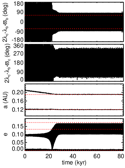
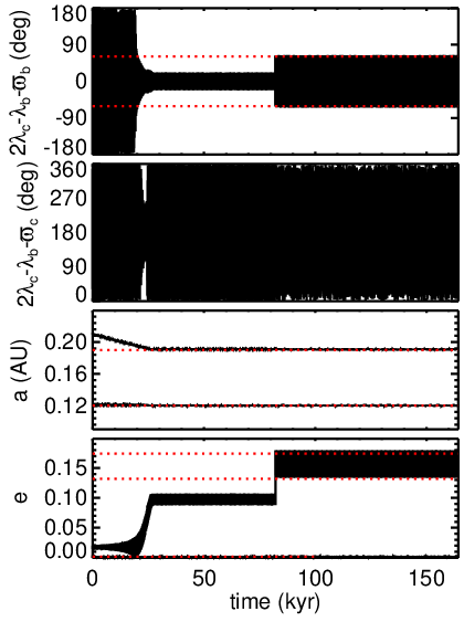
One possible scenario for establishing the resonance is convergent migration of planet c preceded or followed by perturbations of planet b by another body (Fig. 11). We show example simulations that apply a migration force using the user-defined force feature of mercury6 (as described in Wolff et al. 2012); the simulations are done in 3D with initial inclinations set to the present day values. Planet c migrates a short distance (0.8% of its initial semi-major axis) toward planet b and captures b into resonance. In the first example (top), planet b starts with a modestly eccentric (bottom) orbit (). In the second example, planet b starts with a lower eccentricity () and is captured into resonance with a tight libration amplitude. At about 80,000 years, planet b’s orbit is disturbed, which we approximate as an instantaneous change in the magnitude and direction of its eccentricity vector. The first history results in large amplitude libration of the resonant angle involving and the second in circulation; because we are not confident that only circulating resonant angles are compatible with the data, we cannot use this distinction to favor one history over the other.
These example dynamical histories are compatible with in situ formation, but are potentially compatible with long distance migration as well. In the in situ formation scenario, three or more planets form in situ, and planet c migrates a tiny distance toward b. A third planet jostles b – exciting its eccentricity and mutual inclination – before or after c’s migration. In the long distance migration scenario, the disturbing third planet could have migrated earlier. As future work, orbital dynamics simulations could place limits on the properties of this possible third planet. Although we have invoked a third planet in the example scenarios, we have not ruled out the possibility that planet b itself disturbed planet c, in a process separate from migration.
Another hypothesis for the mutual inclination is that it was excited when the planets passed through the 4:2 inclination resonance during migration (Thommes & Lissauer 2003). Precession from the proto-planetary disk can separate the 4:2 inclination resonances from the 2:1 eccentricity resonance. Figure 12 shows a proof of concept simulation where the potential of the proto-planetary disk is approximated as a oblateness term for the stellar potential. A small but significant mutual inclination is excited.

We place planet b and c on a mass-radius plot of warm exoplanets in Fig. 13. TOI-216c has a typical radius for its mass; its bulk density is 0.885 gcm-3. TOI-216b likely also has a typical radius for its mass, but because of its grazing transit (Section II) and the resulting degeneracy with impact parameter, we cannot rule out a large radius that would result in a low density for its mass compared to similar mass planets. Its poorly-constrained bulk density is 0.17 gcm-3.

V Conclusion
TOI-216b and c are now a very precisely characterized (with the exception of planet b’s radius) pair of warm, large exoplanets. Radial velocity measurements using HARPS, FEROS, and PFS broke a degeneracy between mass and eccentricity in the TTV-only fits that was particularly severe before the TESS Extended Mission observations, and an expanded TTV baseline from TESS and an ongoing ground-based transit observing campaign increased the precision of the fits. We can now better assess the consistency of its properties with different theories for formation and evolution of giant planets orbiting close to their stars.
We now know that TOI-216c is a warm Jupiter ( Jupiter masses) with a mass and radius typical of other 10–200 day giant planets (Fig. 13). TOI-216b has a mass similar to Neptune’s (18.4). Its radius is not well constrained due to its grazing transits; its radius may very well be typical for its mass (Fig. 13). Given the large uncertainty in planet b’s radius, no inflation mechanisms or scenarios requiring formation beyond the ice line (e.g., Lee & Chiang 2016) are required to explain either planet’s radius.
Furthermore, we know now that TOI-216b and c are not just near but librating in the 2:1 resonance. The argument involving the longitude of periapse of TOI-216b librates with an amplitude of degrees. TOI-216b has a small but significant free eccentricity . The mutual inclination with respect to TOI-216c is between 1.2–3.9∘ (95% confidence interval). The libration amplitude, free eccentricity, and mutual inclination imply a disturbance of TOI-216b before or after resonance capture, perhaps by an undetected third planet. The orbital properties can be consistent either with in situ formation, with resonance capture through a very short distance migration, or long distance migration. Future origins scenarios must match these precisely constrained properties. Future atmospheric characterization by the James Webb Space Telescope (JWST) may help distinguish between these origin scenarios. If the planet formed outside the water snow line, we expect its C/O ratio to be significantly smaller than that of its host star; in-situ formation, on the other hand, would imply C/O ratios closer to the star (Espinoza et al. 2017). Simulations performed with PandExo (Batalha et al. 2017) show that water features in the spectra that constrain the C/O ratio may be detectable for TOI-216c with the JWST Near Infrared Imager and Slitless Spectrograph (NIRISS), even beneath a moderate cloud layer.
This system will benefit from continued long-term radial-velocity and transit monitoring. Long-term radial velocity monitoring could reveal the presence of additional planets in the system, though stellar activity poses a challenge for detecting low amplitude signals. Observations by the TESS Extended Mission are continuing and will further increase the baseline of observations. The new TESS observations may allow us to better constrain the change in impact parameter tentatively detected here for TOI-216b, allowing for tighter constraints on the mutual inclination.
References
- Agol et al. (2005) Agol, E., Steffen, J., Sari, R., & Clarkson, W. 2005, MNRAS, 359, 567, doi: 10.1111/j.1365-2966.2005.08922.x
- Anderson et al. (2020) Anderson, K. R., Lai, D., & Pu, B. 2020, MNRAS, 491, 1369, doi: 10.1093/mnras/stz3119
- Anglada-Escudé et al. (2010) Anglada-Escudé, G., López-Morales, M., & Chambers, J. E. 2010, ApJ, 709, 168, doi: 10.1088/0004-637X/709/1/168
- Astropy Collaboration et al. (2013) Astropy Collaboration, Robitaille, T. P., Tollerud, E. J., et al. 2013, A&A, 558, A33, doi: 10.1051/0004-6361/201322068
- Astropy Collaboration et al. (2018) Astropy Collaboration, Price-Whelan, A. M., Sipőcz, B. M., et al. 2018, AJ, 156, 123, doi: 10.3847/1538-3881/aabc4f
- Batalha et al. (2017) Batalha, N. E., Mandell, A., Pontoppidan, K., et al. 2017, PASP, 129, 064501, doi: 10.1088/1538-3873/aa65b0
- Boisse et al. (2009) Boisse, I., Moutou, C., Vidal-Madjar, A., et al. 2009, A&A, 495, 959, doi: 10.1051/0004-6361:200810648
- Brahm et al. (2017) Brahm, R., Jordán, A., & Espinoza, N. 2017, PASP, 129, 034002, doi: 10.1088/1538-3873/aa5455
- Brahm et al. (2019) Brahm, R., Espinoza, N., Jordán, A., et al. 2019, AJ, 158, 45, doi: 10.3847/1538-3881/ab279a
- Brown et al. (2013) Brown, T. M., Baliber, N., Bianco, F. B., et al. 2013, Publications of the Astronomical Society of the Pacific, 125, 1031, doi: 10.1086/673168
- Butler et al. (1996) Butler, R. P., Marcy, G. W., Williams, E., et al. 1996, PASP, 108, 500, doi: 10.1086/133755
- Canto Martins et al. (2020) Canto Martins, B. L., Gomes, R. L., Messias, Y. S., et al. 2020, arXiv e-prints, arXiv:2007.03079. https://arxiv.org/abs/2007.03079
- Carter & Winn (2009) Carter, J. A., & Winn, J. N. 2009, ApJ, 704, 51, doi: 10.1088/0004-637X/704/1/51
- Chambers et al. (1996) Chambers, J. E., Wetherill, G. W., & Boss, A. P. 1996, Icarus, 119, 261, doi: 10.1006/icar.1996.0019
- Choksi & Chiang (2020) Choksi, N., & Chiang, E. 2020, MNRAS, doi: 10.1093/mnras/staa1421
- Collins et al. (2017) Collins, K. A., Kielkopf, J. F., Stassun, K. G., & Hessman, F. V. 2017, AJ, 153, 77, doi: 10.3847/1538-3881/153/2/77
- Crane et al. (2006) Crane, J. D., Shectman, S. A., & Butler, R. P. 2006, Society of Photo-Optical Instrumentation Engineers (SPIE) Conference Series, Vol. 6269, The Carnegie Planet Finder Spectrograph, 626931, doi: 10.1117/12.672339
- Crane et al. (2010) Crane, J. D., Shectman, S. A., Butler, R. P., et al. 2010, Society of Photo-Optical Instrumentation Engineers (SPIE) Conference Series, Vol. 7735, The Carnegie Planet Finder Spectrograph: integration and commissioning, 773553, doi: 10.1117/12.857792
- Crane et al. (2008) Crane, J. D., Shectman, S. A., Butler, R. P., Thompson, I. B., & Burley, G. S. 2008, Society of Photo-Optical Instrumentation Engineers (SPIE) Conference Series, Vol. 7014, The Carnegie Planet Finder Spectrograph: a status report, 701479, doi: 10.1117/12.789637
- Cumming (2004) Cumming, A. 2004, MNRAS, 354, 1165, doi: 10.1111/j.1365-2966.2004.08275.x
- Cumming et al. (1999) Cumming, A., Marcy, G. W., & Butler, R. P. 1999, ApJ, 526, 890, doi: 10.1086/308020
- Dawson (2020) Dawson, R. I. 2020, AJ, 159, 223, doi: 10.3847/1538-3881/ab7fa5
- Dawson & Johnson (2012) Dawson, R. I., & Johnson, J. A. 2012, ApJ, 756, 122, doi: 10.1088/0004-637X/756/2/122
- Dawson & Johnson (2018) —. 2018, ARA&A, 56, 175, doi: 10.1146/annurev-astro-081817-051853
- Dawson et al. (2014) Dawson, R. I., Johnson, J. A., Fabrycky, D. C., et al. 2014, ApJ, 791, 89, doi: 10.1088/0004-637X/791/2/89
- Dawson et al. (2019) Dawson, R. I., Huang, C. X., Lissauer, J. J., et al. 2019, AJ, 158, 65, doi: 10.3847/1538-3881/ab24ba
- Deck & Agol (2015) Deck, K. M., & Agol, E. 2015, ApJ, 802, 116, doi: 10.1088/0004-637X/802/2/116
- Dong & Dawson (2016) Dong, R., & Dawson, R. 2016, ApJ, 825, 77, doi: 10.3847/0004-637X/825/1/77
- Edelson & Krolik (1988) Edelson, R. A., & Krolik, J. H. 1988, ApJ, 333, 646, doi: 10.1086/166773
- Espinoza et al. (2017) Espinoza, N., Fortney, J. J., Miguel, Y., Thorngren, D., & Murray-Clay, R. 2017, ApJ, 838, L9, doi: 10.3847/2041-8213/aa65ca
- Feinstein et al. (2019) Feinstein, A. D., Montet, B. T., Foreman-Mackey, D., et al. 2019, PASP, 131, 094502, doi: 10.1088/1538-3873/ab291c
- Foreman-Mackey (2018) Foreman-Mackey, D. 2018, Research Notes of the American Astronomical Society, 2, 31, doi: 10.3847/2515-5172/aaaf6c
- Foreman-Mackey et al. (2017) Foreman-Mackey, D., Agol, E., Ambikasaran, S., & Angus, R. 2017, AJ, 154, 220, doi: 10.3847/1538-3881/aa9332
- Foreman-Mackey et al. (2019) Foreman-Mackey, D., Czekala, I., Luger, R., et al. 2019, dfm/exoplanet: exoplanet v0.2.1, doi: 10.5281/zenodo.3462740
- Foreman-Mackey et al. (2013) Foreman-Mackey, D., Hogg, D. W., Lang, D., & Goodman, J. 2013, PASP, 125, 306, doi: 10.1086/670067
- Frelikh et al. (2019) Frelikh, R., Jang, H., Murray-Clay, R. A., & Petrovich, C. 2019, ApJ, 884, L47, doi: 10.3847/2041-8213/ab4a7b
- Gazak et al. (2012) Gazak, J. Z., Johnson, J. A., Tonry, J., et al. 2012, Advances in Astronomy, 2012, 697967, doi: 10.1155/2012/697967
- Huang et al. (2016) Huang, C., Wu, Y., & Triaud, A. H. M. J. 2016, ApJ, 825, 98, doi: 10.3847/0004-637X/825/2/98
- Jenkins et al. (2002) Jenkins, J. M., Caldwell, D. A., & Borucki, W. J. 2002, ApJ, 564, 495, doi: 10.1086/324143
- Jenkins et al. (2010) Jenkins, J. M., Caldwell, D. A., Chandrasekaran, H., et al. 2010, ApJ, 713, L87, doi: 10.1088/2041-8205/713/2/L87
- Jenkins et al. (2016) Jenkins, J. M., Twicken, J. D., McCauliff, S., et al. 2016, in Proc. SPIE, Vol. 9913, Software and Cyberinfrastructure for Astronomy IV, 99133E, doi: 10.1117/12.2233418
- Jensen (2013) Jensen, E. 2013, Tapir: A web interface for transit/eclipse observability, Astrophysics Source Code Library. http://ascl.net/1306.007
- Jordán et al. (2020) Jordán, A., Brahm, R., Espinoza, N., et al. 2020, AJ, 159, 145, doi: 10.3847/1538-3881/ab6f67
- Kaufer et al. (1999) Kaufer, A., Stahl, O., Tubbesing, S., et al. 1999, The Messenger, 95, 8
- Kipping et al. (2019) Kipping, D., Nesvorný, D., Hartman, J., et al. 2019, MNRAS, 486, 4980, doi: 10.1093/mnras/stz1141
- Kipping (2013a) Kipping, D. M. 2013a, MNRAS, 435, 2152, doi: 10.1093/mnras/stt1435
- Kipping (2013b) —. 2013b, MNRAS, 435, 2152, doi: 10.1093/mnras/stt1435
- Korth (2020) Korth, J. 2020, PhD thesis. http://www.uni-koeln.de/
- Kürster et al. (2015) Kürster, M., Trifonov, T., Reffert, S., Kostogryz, N. M., & Rodler, F. 2015, A&A, 577, A103, doi: 10.1051/0004-6361/201525872
- Lee & Chiang (2016) Lee, E. J., & Chiang, E. 2016, ApJ, 817, 90, doi: 10.3847/0004-637X/817/2/90
- Lee & Peale (2002) Lee, M. H., & Peale, S. J. 2002, ApJ, 567, 596, doi: 10.1086/338504
- Li et al. (2019) Li, J., Tenenbaum, P., Twicken, J. D., et al. 2019, PASP, 131, 024506, doi: 10.1088/1538-3873/aaf44d
- Lithwick & Naoz (2011) Lithwick, Y., & Naoz, S. 2011, ApJ, 742, 94, doi: 10.1088/0004-637X/742/2/94
- Lithwick et al. (2012) Lithwick, Y., Xie, J., & Wu, Y. 2012, ApJ, 761, 122, doi: 10.1088/0004-637X/761/2/122
- Luger et al. (2019) Luger, R., Agol, E., Foreman-Mackey, D., et al. 2019, AJ, 157, 64, doi: 10.3847/1538-3881/aae8e5
- MacDonald & Dawson (2018) MacDonald, M. G., & Dawson, R. I. 2018, AJ, 156, 228, doi: 10.3847/1538-3881/aae266
- Mandel & Agol (2002) Mandel, K., & Agol, E. 2002, ApJ, 580, L171, doi: 10.1086/345520
- Markwardt (2009) Markwardt, C. B. 2009, in Astronomical Society of the Pacific Conference Series, Vol. 411, Astronomical Data Analysis Software and Systems XVIII, ed. D. A. Bohlender, D. Durand, & P. Dowler, 251. https://arxiv.org/abs/0902.2850
- Mayor et al. (2003) Mayor, M., Pepe, F., Queloz, D., et al. 2003, The Messenger, 114, 20
- McCully et al. (2018) McCully, C., Volgenau, N. H., Harbeck, D.-R., et al. 2018, in Society of Photo-Optical Instrumentation Engineers (SPIE) Conference Series, Vol. 10707, Proc. SPIE, 107070K, doi: 10.1117/12.2314340
- McQuillan et al. (2014) McQuillan, A., Mazeh, T., & Aigrain, S. 2014, ApJS, 211, 24, doi: 10.1088/0067-0049/211/2/24
- Millholland et al. (2018) Millholland, S., Laughlin, G., Teske, J., et al. 2018, AJ, 155, 106, doi: 10.3847/1538-3881/aaa894
- Mustill et al. (2015) Mustill, A. J., Davies, M. B., & Johansen, A. 2015, ApJ, 808, 14, doi: 10.1088/0004-637X/808/1/14
- Nesvorný & Vokrouhlický (2016) Nesvorný, D., & Vokrouhlický, D. 2016, ApJ, 823, 72, doi: 10.3847/0004-637X/823/2/72
- Parviainen (2015) Parviainen, H. 2015, MNRAS, 450, 3233, doi: 10.1093/mnras/stv894
- Rein & Liu (2012) Rein, H., & Liu, S. F. 2012, A&A, 537, A128, doi: 10.1051/0004-6361/201118085
- Rein & Spiegel (2015) Rein, H., & Spiegel, D. S. 2015, MNRAS, 446, 1424, doi: 10.1093/mnras/stu2164
- Salvatier et al. (2016) Salvatier, J., Wiecki, T. V., & Fonnesbeck, C. 2016, PeerJ Computer Science, 2, e55
- Schneider et al. (2011) Schneider, J., Dedieu, C., Le Sidaner, P., Savalle, R., & Zolotukhin, I. 2011, A&A, 532, A79, doi: 10.1051/0004-6361/201116713
- Smith et al. (2012) Smith, J. C., Stumpe, M. C., Van Cleve, J. E., et al. 2012, PASP, 124, 1000, doi: 10.1086/667697
- Stumpe et al. (2014) Stumpe, M. C., Smith, J. C., Catanzarite, J. H., et al. 2014, PASP, 126, 100, doi: 10.1086/674989
- Tamayo et al. (2020) Tamayo, D., Rein, H., Shi, P., & Hernand ez, D. M. 2020, MNRAS, 491, 2885, doi: 10.1093/mnras/stz2870
- Theano Development Team (2016) Theano Development Team. 2016, arXiv e-prints, abs/1605.02688. http://arxiv.org/abs/1605.02688
- Thommes & Lissauer (2003) Thommes, E. W., & Lissauer, J. J. 2003, ApJ, 597, 566, doi: 10.1086/378317
- Twicken et al. (2018) Twicken, J. D., Catanzarite, J. H., Clarke, B. D., et al. 2018, PASP, 130, 064502, doi: 10.1088/1538-3873/aab694
- Van Eylen et al. (2019) Van Eylen, V., Albrecht, S., Huang, X., et al. 2019, AJ, 157, 61, doi: 10.3847/1538-3881/aaf22f
- Wolff et al. (2012) Wolff, S., Dawson, R. I., & Murray-Clay, R. A. 2012, ApJ, 746, 171, doi: 10.1088/0004-637X/746/2/171
- Zechmeister & Kürster (2009) Zechmeister, M., & Kürster, M. 2009, A&A, 496, 577, doi: 10.1051/0004-6361:200811296
| RV | BIS | Inst. | Note | |||
|---|---|---|---|---|---|---|
| -2450000 | (m s-1) | (m s-1) | (m s-1) | (m s-1) | ||
| 8449.70722 | 36690.0 | 7.8 | -16.0 | 12.0 | FEROS | |
| 8450.62181 | 36709.1 | 8.0 | -12.0 | 12.0 | FEROS | |
| 8450.75019 | 36686.8 | 8.3 | -35.0 | 12.0 | FEROS | |
| 8451.72708 | 36706.3 | 7.7 | -21.0 | 12.0 | FEROS | |
| 8451.74212 | 36696.3 | 7.2 | -44.0 | 11.0 | FEROS | |
| 8451.75750 | 36694.2 | 7.2 | -25.0 | 11.0 | FEROS | |
| 8452.77587 | 36713.0 | 7.6 | -48.0 | 11.0 | FEROS | |
| 8464.76381 | 36754.4 | 8.7 | 11.0 | 11.0 | HARPS | |
| 8464.81000 | 36744.7 | 10.3 | 19.0 | 13.0 | HARPS | |
| 8465.73524 | 36759.3 | 4.1 | 9.0 | 5.0 | HARPS | |
| 8465.75656 | 36753.4 | 4.6 | 5.0 | 6.0 | HARPS | |
| 8466.72641 | 36733.7 | 6.4 | -5.0 | 8.0 | HARPS | |
| 8466.74802 | 36730.1 | 7.4 | -11.0 | 10.0 | HARPS | |
| 8467.74159 | 36714.5 | 7.9 | -35.0 | 12.0 | FEROS | |
| 8468.67914 | 10.49 | 1.11 | . | . | PFS | |
| 8468.74406 | 36727.7 | 7.7 | 0.0 | 12.0 | FEROS | |
| 8472.76399 | 1.38 | 1.23 | . | . | PFS | |
| 8476.74101 | -23.94 | 1.18 | . | . | PFS | |
| 8479.63075 | -33.40 | 1.15 | . | . | PFS | |
| 8480.71817 | -33.50 | 1.33 | . | . | PFS | |
| 8481.63918 | 36681.1 | 5.6 | 3.0 | 7.0 | HARPS | |
| 8481.66088 | 36670.1 | 4.9 | -7.0 | 6.0 | HARPS | |
| 8482.63750 | 36690.5 | 4.1 | 2.0 | 5.0 | HARPS | |
| 8482.65892 | 36684.0 | 4.3 | -1.0 | 6.0 | HARPS | |
| 8483.63626 | 36702.2 | 4.3 | -8.0 | 6.0 | HARPS | |
| 8483.65821 | 36704.1 | 4.1 | 11.0 | 5.0 | HARPS | |
| 8483.76291 | 36668.1 | 8.0 | -1.0 | 12.0 | FEROS | |
| 8485.70826 | 36650.9 | 13.9 | 47.0 | 19.0 | FEROS | |
| 8493.72558 | 36735.9 | 9.0 | -11.0 | 13.0 | FEROS | |
| 8497.62083 | 36696.5 | 7.8 | -40.0 | 12.0 | FEROS | |
| 8501.68699 | 34.11 | 1.72 | . | . | PFS | |
| 8503.65356 | 36813.1 | 14.3 | 64.0 | 19.0 | FEROS | Outlier |
| 8504.65888 | 36684.4 | 9.0 | -61.0 | 13.0 | FEROS | |
| 8507.66569 | -11.68 | 2.42 | . | . | PFS | |
| 8510.68697 | -27.18 | 1.88 | . | . | PFS | |
| 8521.56775 | 36625.2 | 7.6 | 5.0 | 11.0 | FEROS | Outlier |
| 8528.60948 | 46.62 | 1.76 | . | . | PFS | |
| 8529.58589 | 45.56 | 1.65 | . | . | PFS | |
| 8542.55798 | 36659.1 | 8.7 | -44.0 | 13.0 | FEROS | |
| 8543.54347 | 36640.3 | 7.4 | -6.0 | 11.0 | FEROS | |
| 8544.61674 | 36663.3 | 7.8 | -26.0 | 12.0 | FEROS | |
| 8545.57452 | 36676.3 | 7.6 | -3.0 | 11.0 | FEROS | |
| 8546.58251 | 36714.8 | 9.7 | 38.0 | 14.0 | FEROS | |
| 8547.53676 | 36635.1 | 7.9 | -17.0 | 12.0 | FEROS | |
| 8548.58309 | 36652.2 | 7.7 | 23.0 | 12.0 | FEROS | |
| 8550.61335 | 36613.1 | 8.2 | -62.0 | 12.0 | FEROS | |
| 8551.62488 | 36637.6 | 11.4 | -26.0 | 16.0 | FEROS | |
| 8554.56409 | 36707.0 | 8.9 | -38.0 | 13.0 | FEROS | |
| 8557.56708 | 36713.0 | 9.2 | -4.0 | 13.0 | FEROS | |
| 8708.90979 | 28.50 | 2.14 | . | . | PFS | |
| 8711.89325 | 12.38 | 2.62 | . | . | PFS | |
| 8714.92414 | -16.98 | 2.14 | . | . | PFS | |
| 8742.88505 | 19.06 | 2.19 | . | . | PFS | |
| 8764.84159 | 36736.7 | 5.2 | -1.0 | 7.0 | HARPS | |
| 8766.79176 | 36750.6 | 6.4 | 3.0 | 8.0 | HARPS | |
| 8767.86802 | 29.71 | 1.98 | . | . | PFS | |
| 8777.79725 | 36695.8 | 23.5 | 23.0 | 31.0 | HARPS | |
| 8914.55281 | 21.41 | 2.73 | . | . | PFS | |
| 8920.52884 | -5.82 | 1.77 | . | . | PFS | |
| 8923.53817 | -33.84 | 1.94 | . | . | PFS |
| Parameter | Value |
|---|---|
| 0.77 | |
| () | 0.061381 |
| 17.096824 | |
| 0.15830 | |
| (deg.) | 292.55926 |
| (deg) | 82.329609 |
| (deg) | 0 |
| (deg) | 88.594066 |
| () | 0.55454 |
| 34.551590 | |
| 0.0056764 | |
| (deg.) | 200.93260 |
| (deg) | 27.931018 |
| (deg) | -0.20544800 |
| (deg) | 89.785658 |