Discrete-Time Consensus Networks: Scalability, Grounding and Countermeasures

A graph is denoted by $\mathcal{{G}}=(\mathcal{{V}},\mathcal{{E}})$, where $\mathcal{{V}}=\{1,\cdots,N\}$ is the node set and $\mathcal{{E}}$ is the edge set. A graph is undirected if the edge set consists of unordered pairs $(i,j)\in\mathcal{E},i,j=1,\cdots,N$, if there is communication between nodes $i$ and $j$. A graph is called simple if there are no loops ($(i,i)\not\in\mathcal{E}~\forall i\in\mathcal{V}$) and each edge is present only once in $\mathcal{E}$. A graph family $\{\mathcal{G}_{N}\}$ is a sequence of graphs with increasing number of nodes, i.e., $N\rightarrow\infty$.

If $(i,j)\in\mathcal{{E}}$, node $j$ is called a neighbor of node $i$. $\mathcal{N}_{i}$ denotes the neighbor set of node $i$ with respect to $\mathcal{V}$. The degree of a node $i$ is equal to the number of neighbors node $i$ has, i.e., $d_{i}=|\mathcal{N}_{i}|$. The degree matrix $\mathcal{D}$ is a diagonal matrix having the elements $d_{i}$ on the diagonal. A graph is called $d$-regular if the degree of each node is equal to $d$, and is called non-regular if it is not a regular graph.

Let $\mathcal{A}=[\alpha_{ij}]_{i,j=1}^{N}\in\mathbb{R}^{N\times N}$ be the weighted adjacency matrix of ${\mathcal{G}}$ with $i,j=1,\cdots,N$, $\alpha_{ii}=0$, and $\alpha_{ij}=\frac{1}{d_{i}}$ $\Leftrightarrow$ $(j,i)\in\mathcal{E}$. The random walk normalised Laplacian matrix $L=[l_{ij}]\in\mathbb{R}^{N\times N}$ associated with $\mathcal{G}$ is defined as $l_{ii}=1$ and $l_{ij}=-\alpha_{ij},i\neq j$, we have $L=I_{N}-\mathcal{A}$. The symmetric normalized adjacency matrix is defined as $\mathcal{A}_{sym}=\mathcal{D}^{\frac{1}{2}}\mathcal{A}\mathcal{D}^{-\frac{1}{2}}$ and its associated Laplacian matrix $L_{sym}$ is denoted by $L_{sym}=\mathcal{D}^{\frac{1}{2}}L\mathcal{D}^{-\frac{1}{2}}=I_{N}-\mathcal{A}_{sym}$.

Throughout this paper, we consider undirected, simple, and connected communication graphs. The eigenvalues of $L_{sym}$ and $L$ agree since they are similar and are denoted by $\lambda_{i}\in\mathbb{R},\ i=1,\cdots,N$ and in an ascending order are written as $0=\lambda_{1}\leq\lambda_{2}\leq\cdots\leq\lambda_{N}$ and $\lambda_{i}\leq 2$ for $i=2,\dots,N$. We denote $\lambda_{\max}(\boldsymbol{M})$ and $\lambda_{\min}(\boldsymbol{M})$ by the largest and the smallest positive eigenvalue of a symmetrical matrix $\boldsymbol{M}$, respectively; see e.g., $\lambda_{\min}(L)=\lambda_{2}$. The second smallest eigenvalue of the Laplacian matrix, $\lambda_{2}$, is called the algebraic connectivity of the graph. As in [4], $\rho=\lambda_{2}/\lambda_{N}$, is called the eigenratio of an undirected graph. We consider throughout the paper graph families, $c^{\prime}$-expanders, with the so-called minimum $c^{\prime}$-algebraic connected property.

Generally, as the number of nodes increases while keeping a constant nodal degree, the algebraic connectivity tends towards zero. This means that with increasing $N$ the graph loses its connectivity and the performance of the consensus algorithm deteriorates. A minimum $c^{\prime}$-algebraic connected graph family does not exhibit this decrease in connectivity while maintaining a bounded nodal degree.

We consider a discrete-time multi-agent system where $N$ agents communicate among each other to achieve consensus on their states in a leader-less architecture. Each agent is governed by a discrete-time dynamic system given in the form of

where $x_{i}\in\mathbb{R}^{n}$, $u_{i}\in\mathbb{R}$ denote the system state and control input of the $i^{th}$ agent, $A\in\mathbb{R}^{n\times n}$, $B\in\mathbb{R}^{n\times 1}$. $\mathbb{Z}^{+}$ denotes the set of nonnegative integers $\mathbb{Z}^{+}=\{0,1,\cdots\}$. The standard consensus algorithm is adopted as follows,

where $K\in\mathbb{R}^{1\times n}$ is the control gain matrix, $\alpha_{ij}$ the $ij$-th entry of the adjacency matrix $\mathcal{A}$.

The multi-agent consensus network composed of (1) and (2) can be expressed in the following compact form

where $x=[x_{1}^{T},\dots,x_{N}^{T}]^{T}$ and $\otimes$ denotes the Kronecker product.

Throughout the paper we assume the following.

It is known that a necessary and sufficient condition for consensus of system (3) is that there exists $K$ such that $A-\lambda_{i}BK$ is Schur (i.e. all its eigenvalues are inside the open unit circle) for $i=2,\dots,N$ [4]. Under Assumption 1, consider a minimum $c^{\prime}$-algebraic connected graph family where $c^{\prime}$ should satisfy as in [17]

Then, we design

where $R\geq 0$, $P=P^{T}>0$ is a solution to the modified algebraic Riccati inequality

with $\sigma$ satisfying

From [17], we select $\epsilon$ to satisfy

which guarantees that the gain $K$ in (5) is such that the network achieves consensus.

Grounding a node of a network turns the node into one that influences other nodes but is not affected in return. In a multi-agent context, this grounded node acts as a leader and converts the whole network from a leaderless architecture to a leader-following one. In other contexts, the grounded node can be interpreted as a “stubborn agent”[18]. As mentioned previously, the terminology stems from its application in power networks where grounding a node means literally connecting the bus to ground forcing the state, in this case the voltage, to be set to $0$. To put this concept in a general framework using networked control language, we consider three different ways to ground a node. These different ways will have different influences on network consensus. Without loss of generality, we suppose grounding happens to node 1.

A first form of grounding consists in fixing node 1’s state $x_{1}(k)$ at some time $k_{0}$ to be either its current state or any constant value $\bar{c}$ in the proper dimension. Then, $x_{1}(k)=\bar{c}$ for all $k\geq k_{0}$. The closed-loop system for the remaining nodes can be described as

where $\bar{L}$ is the grounded Laplacian [13] obtained by removing the first row and column of $L$, $\Lambda$ is a diagonal matrix with diagonal entries equal to $\alpha_{i1}$ and $\bar{x}$ is obtained from $x$ by removing the states of node 1. If $(I_{N-1}\otimes A-\bar{L}\otimes BK)$ is Schur, then $\bar{x}$ will approach $(I_{n(N-1)}-(I_{N-1}\otimes A-\bar{L}\otimes BK))^{-1}(\Lambda\otimes BK)(1_{N-1}\otimes\bar{c})$.

A second form of grounding consists in cutting the control channel so that $u_{1}=0$, and optionally change the dynamics of node 1. Then, the first node’s dynamics are $x_{1}(k+1)=\bar{A}x_{1}(k)$. If $\bar{A}=A$, the consensus trajectory will be the same as that of $x_{1}$ if grounding happens after the consensus was achieved; the consensus trajectory will be different from that of $x_{1}$ if grounding happens before the consensus is achieved.

A third form of grounding consists in taking control of $u_{1}$ such that $x_{1}$ is steered towards a deliberately designed trajectory, for example, a certain setpoint $c_{0}$. Specifically, a stabilizing controller $u_{1}=-K_{1}x_{1}+c_{1}$ makes the closed-loop dynamics of node 1 $x_{1}(k+1)=(A-BK_{1})x_{1}(k)+Bc_{1}$ with $(A-BK_{1})$ Schur. The closed-loop system for the remaining nodes will be

If $(I_{N-1}\otimes A-\bar{L}\otimes BK)$ is Schur, all states of the remaining nodes will approach $c_{0}=(I-(A-BK_{1}))^{-1}Bc_{1}$.

Note that to analyze the consequences of grounding, a key system matrix to be analyzed is $(I_{N-1}\otimes A-\bar{L}\otimes BK)$. Actually, when letting $x_{1}=\mathbf{0}_{n}$, where $\mathbf{0}_{n}$ denotes the column vector of $n$ zeros, the closed-loop system for the remaining nodes will be

The performance of the grounded network will be directly related to the grounded Laplacian $\bar{L}$. We denote the eigenvalues of $\bar{L}$ as $\bar{\lambda}_{i}$ and they are numbered as $0<\bar{\lambda}_{1}\leq\dots\leq\bar{\lambda}_{N-1}$. The smallest eigenvalue $\bar{\lambda}_{1}$ is known as grounded algebraic connectivity. We denote the ratio $\bar{\rho}=\bar{\lambda}_{1}/\bar{\lambda}_{N-1}$ by grounded eigenratio.

In the following sections, we present results and discussions on spectral properties of $\bar{L}$ in regard to scalability, consensus performance, and consensusability. Specifically, we address the following problems.

Scalability, performance, and consensusability: Suppose the network graph has good scaling properties, that is, it is possible to achieve consensus as the network size grows large. Is this property preserved when a node is grounded. Is the convergence rate to consensus afffected by grounding. And, also how is the consensusability condition of Assumption 1 affected when the system dynamics are unstable. Can consensusability be lost.

Possible countermeasuers: When interpreting grounding as an attack, what are the possible countermeasures that can be taken to correct or minimise the effect of grounding. How to choose an optimal countermeasure to recover the performance or in the worst case the consensusability. One countermeasure we will in particular investigate is the grounding of additional nodes. We investigate how to select effectively which nodes to ground and how many nodes should be grounded to recover the consensus performance.

It is possible to design the controller beforehand to be resilient to grounding. At the stage of controller design, we select $K$ such that $(I_{N-1}\otimes A-\bar{L}\otimes BK)$ is Schur for every $\bar{L}$ resulting from grounding the $i{th}$ node, for $i=1,\dots,N$. Then, check that $K$ also stabilizes $(A-\lambda_{i}BK)$ for $i=2,\dots,N$. To guarantee the existence of such a grounding-resilient controller, Assumption 4 needs to hold with the eigenratio $\rho$ being replaced by the smallest grounded eigenratio among all those resulting from grounding the $i$th node, $i=1,\dots,N$.

It is possible to take the following actions:

1. 1.

   Suppose the grounded network is consensusable with respect to the agent dynamics. Then, redesign the controller after grounding such that $(I_{N-1}\otimes A-\bar{L}\otimes BK)$ is Schur. Furthermore, if the grounded algebraic connectivity is lower bounded by $c^{\prime}_{g}$ and $c^{\prime}_{g}>\frac{2(1-\tilde{\sigma})}{1+\tilde{\sigma}}$, then, consensus can be achieved by (5) with $\sigma$ and $\epsilon$ selected in (7) and (8) by replacing $c^{\prime}$ with $c^{\prime}_{g}$.

2. 2.

   Suppose the grounded network is unconsensusable with respect to the agent dynamics and the grounded node can be detected. Then we can isolate the grounded node by cutting the connections between the grounded node with all its neighbors. If the rest of the network remains minimum $c^{\prime}$-algebraic connected, not only the consensusability can be recovered but also consensus can be achieved by the original non-grounded control design without reconfiguration.

3. 3.

   Suppose the grounded network is unconsensusable with respect to the agent dynamics. If the system dynamics are unstable, and consensusability is lost, then there does not exist a $K$ to stabilize $(I_{N-1}\otimes A-\bar{L}\otimes BK)$. Neither redesign nor predesign the controller for grounding will work in this case. We then propose a possible approach to regain the consensusability by deliberately grounding more nodes to increase the upper bounds for the allowable unstable dynamics. This may sound counter-intuitive, but it will be seen from the following Lemma 5.1 that by grounding more nodes, the grounded algebraic connectivity increases (or does not decrease), and the spectral radius of the grounded Laplacian decreases (or does not increase), thus leading to a potential increase in eigenratio and larger allowable region for the dynamics to be unstable.

Lemma 5.1 considered, without loss of generality, the first $m$ (or $q$) rows/columns but the results hold for any group of $m$ (or $q$).

It is also worth mentioning that the result in Lemma 5.1 can be obtained by noticing the eigenvalue interlacing theorem. We provide the self-contained proof here for the convenience of the readers.

When the network has $m$ nodes grounded, the upper bound of the smallest eigenvalue of the resulting grounded Laplacian $\bar{L}^{(m)}$ can be obtained by straightforwardly extending Lemma 4.1 as folows.

The selection of an additional node to ground is here aimed at achieving the maximal increase of the grounded algebraic connectivity. It is worth mentioning that when the consensusability of a network is lost after grounding, the additional node to ground should be chosen to attempt to recover the eigenratio. However, when the grounded network is still consensusable, then the additional node to ground can be selected to achieve the highest grounded algebraic connectivity to improve the scalability and consensus performance.

In this section, we thus focus on how to choose an additional node from nodes $2$ to $N$ to be grounded to yield a maximal increase of the grounded algebraic connectivity for $c^{\prime}$-expander $d$-regular graphs. This problem can be formulated as follows:

where $\bar{L}(j)\in\mathbb{R}^{(N-1)\times(N-1)}$ denotes the double grounded Laplacian and is obtained by replacing the $j$th row and column of $\bar{L}$ by zeros, which also means by replacing the $(j+1)$th row and column of $L$ by zeros after grounding the first node. Since the graphs considered are $d$-regular, then $L$, $\mathcal{A}$ and their principal sub-matrices are all symmetric. Let the grounded adjacency matrix be $\bar{\mathcal{A}}$ obtained by removing the first row and the first column of $\mathcal{A}$, $\bar{\mathcal{A}}(j)$ obtained by replacing the $j$th row and column of $\bar{\mathcal{A}}$ by zeros. One has $\bar{L}=I_{N-1}-\bar{\mathcal{A}}$, $\bar{L}(j)=I_{N-1}-e_{j}e_{j}^{T}-\bar{\mathcal{A}}(j)$, where $e_{j}\in\mathbb{R}^{N-1}$ denotes a column vector with all elements being $0$ except the $j$th element being $1$. The eigenvalues of $\bar{L}(j)$ are denoted by $0=\bar{\lambda}_{0}^{\prime}<\bar{\lambda}_{1}^{\prime}\leq\bar{\lambda}_{2}^{\prime}\leq\cdots\leq\bar{\lambda}_{N-2}^{\prime}$, the eigenratio by $\bar{\rho}^{\prime}=\frac{\bar{\lambda}_{1}^{\prime}}{\bar{\lambda}_{N-2}^{\prime}}$.

The ‘max-min’ problem described in (26) appears to be hard as the solution relates to the structure of the double grounded Laplacian $\bar{L}(j)$. We then seek practical ways to select effectively the best node to ground without checking all the $\lambda_{\min}(\bar{L}(j))$ for $j=1,\dots,N-1$. To this end, we first define that a node is in the $i$-th layer if its shortest path to the grounded node has length $i$. A node is said to be in the highest layer if its shortest path to the grounded node has the longest length, with $\ell$ being the longest length. We start by reordering nodes by layers resulting in the following reordered adjacency matrix,

where $1_{n}$ denotes the column vector of $n$ ones, $\mathcal{A}_{j}$, $j=1,\dots,\ell$, denotes the interconnection of nodes in the $j$th layer, $\mathcal{S}_{j,j+1}$ represents the interconnection between nodes in the $j$th layer and those in the $(j+1)$th layer. In this permutation, ${\mathcal{A}}_{{ord}}$ is block tri-diagonal. After grounding of node $1$ occurs, the grounded reordered adjacency matrix $\bar{\mathcal{A}}_{{ord}}$ is obtained by removing the first row and the first column of $\mathcal{A}_{ord}$. One has

Consider the vector $v_{1}=\mathbf{1}_{N-1}$ and $\bar{\mathcal{A}}_{ord}(j)$ denotes the double grounded adjacency matrix obtained by replacing the $j$th row and the $j$th column of $\bar{\mathcal{A}}_{ord}$ by zeros. Then, the maximum eigenvalue of the reordered adjacency matrix can be bounded as

Note that

Minimising the lower bound (46) will allow more ‘room’ for minimising $\lambda_{\max}(\bar{\mathcal{A}}_{ord}(j))$ thus maximising $\lambda_{\min}(\bar{L}(j))$ as $\lambda_{\max}(\bar{\mathcal{A}}(j))=\lambda_{\max}(\bar{\mathcal{A}}_{ord}(j))$. Selecting $j=j^{*}$ such that

then the lower bound can be minimised. Noting that $\psi_{j}=v_{1}^{T}(e_{j}e_{j}^{T}\bar{\mathcal{A}}_{ord}+\bar{\mathcal{A}}_{ord}e_{j}e_{j}^{T})v_{1}$ is the addition of the $j$th row sum and $j$th column sum, $\psi_{j\in\mathcal{N}_{1}}$ is less than $\psi_{j\in\mathcal{V}/{\mathcal{N}}_{1}}$, since, from (6.1), $\psi_{j\in\mathcal{N}_{1}}-\psi_{j\in\mathcal{V}/{\mathcal{N}}_{1}}=\frac{-2}{d}$. Then, we conclude that the neighboring nodes are worse candidates to ground than non-neighboring nodes when considering the available ‘room’ to recover the grounded eigenvalue. This suggests that the selection of the additional node to be grounded relates to the distance from the first grounded node, namely, node $1$. In fact, Monte Carlos simulations suggest that the best additional node to ground usually appears in the highest two layers $\ell$ and $\ell-1$. Motivated by these findings, we propose the following algorithm to assist us in selecting an additional node to ground aiming at recovering the algebraic connectivity.

We illustrate this algorithm by the following example as seen in Fig. 1. This figure shows the distribution of the double grounded algebraic connectivity $\bar{\lambda}_{1}^{\prime}$ and double grounded eigenratio $\bar{\rho}^{\prime}$. To produce this figure, we use the algorithm in [21] to generate $20$ graphs of $100$ agents with degree $6$. For each graph and each layer, we plot the maximum and minimum values of the double grounded algebraic connectivity (top plot) and the maximum and minimum values of the double grounded eigenratio (bottom plot). We can see that the range of $\bar{\lambda}_{1}^{\prime}$ appears to be in ‘belt’-shape in terms of which layer the node is located. The figure shows that the worst node, that is the node with the minimal $\bar{\lambda}_{1}^{\prime}$ is always a neighboring node of the grounded node. The best node appears most likely in the highest layer $\ell$, and sometimes in the layer $\ell-1$. If we change the network by allowing different degrees, the percentage of the best node in terms of $\bar{\lambda}_{1}^{\prime}$ and $\bar{\rho}^{\prime}$ appearing in the $\ell$th layer or in the ($\ell-1$)th layer can be seen in Fig.2. This was obtained by randomly generating $100$ graphs using the algorithm in [21] for each case. We fix the network size $N=100$ and have the degree changing as $d=5,15,\dots,50$. When the degree increases up to half of the network size, the best node is almost always in the highest layer. Fig. 3 shows the percentage of the best node appearing in each layer when we fix the degree $d=6$, and change $N$ from $10,20,\dots,400$.

Next, we recall Perron-Frobenius theorem for non-negative matrices (with all the entries non-negative).

Consider $\bar{\mathcal{A}}$, which is non-negative, and assume the remaining network (excluding node $1$) is strongly connected. Then $\lambda_{\max}(\bar{\mathcal{A}})$ is real and unique, and its corresponding normalized eigenvector $v_{\max}$ has positive elements with $v_{\max}^{T}\textbf{1}_{N-1}=1$. Similar to the analysis leading to Algorithm 1, we are interested in choosing $j$ to minimise $\lambda_{\max}(\bar{\mathcal{A}}(j))$. One has

then,

where $v_{\max,j}$ represents the $j$th element of $v_{\max}$. Let $\tilde{\psi}_{j}=[(v_{\max}^{T}\bar{\mathcal{A}}e_{j})v_{\max,j}]$. Selecting $j=j^{*}$ such that $j^{*}=\arg\max_{j=1,\dots,N-1}\tilde{\psi}_{j}$, the lower bound in (49) will be minimized. As discussed before, this gives more ‘room’ for minimising $\lambda_{\max}(\bar{\mathcal{A}}(j))$ thus maximising $\lambda_{\min}(\bar{L}(j))$. Note that $\bar{\mathcal{A}}e_{j}$ represents the $j$th column of $\bar{\mathcal{A}}$ which contains mostly $0$ entries if the network is sparse. In this case, the major contribution comes from choosing the maximal $v_{\max,j}$. We can see that $\bar{\mathcal{A}}^{k}\mathbf{1}_{N-1}$ approaches $v_{\max}$, as $k\to\infty$. Thus we propose to choose the maximum element of $\bar{\mathcal{A}}^{\ell}\mathbf{1}_{N-1}$ as an approximation of $v_{\max,j}$. Based on above analysis, we propose the following algorithm to select the best node to ground.

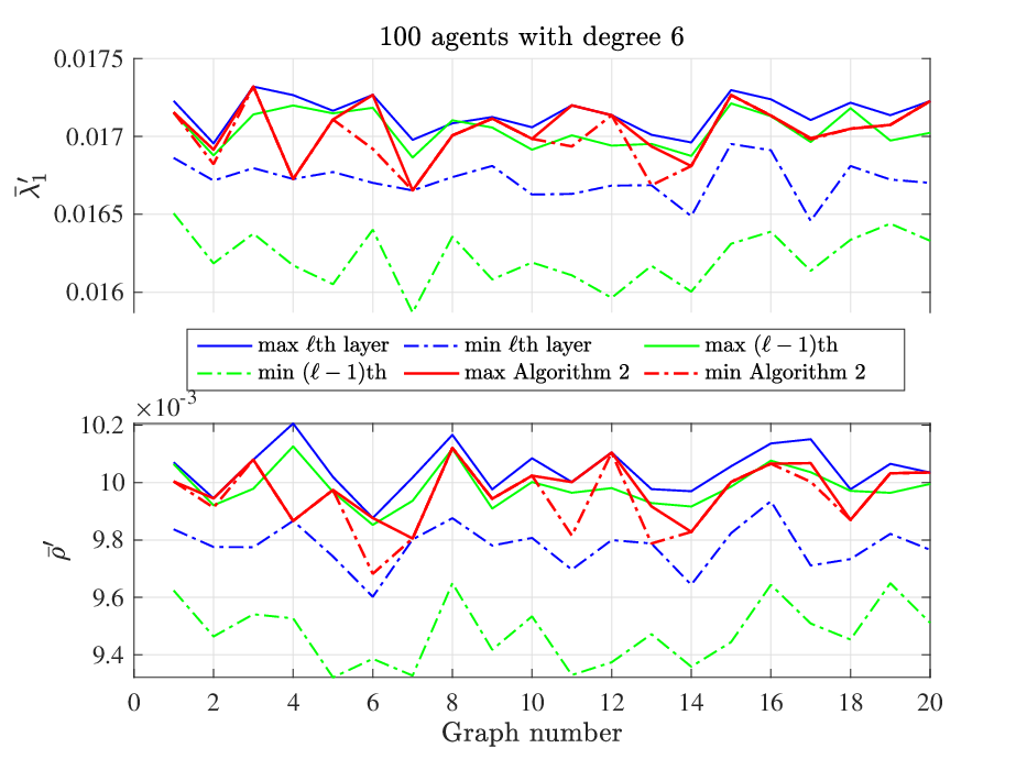
It is noted that Algorithm 2 essentially picks $j$ to maximise an approximation of $v_{\max,j}$. Fig. 4 validates the usefulness of Algorithm 2 by showing that the smallest eigenvalue $\bar{\lambda}_{1}^{\prime}$ of the resulting double grounded matrix $\bar{L}(j)$ corresponding to the selected nodes is very close to that corresponding to the best nodes. Note that Fig. 4 is generated in the same way as Fig. 1, with the addition of the selection achieved by Algorithm 2.

Finally, we observe that, $\ell$ is usually not very large ($<10$) as seen in Fig. 5, which shows the number of the highest layer $\ell$ as a function of network size for two different degrees. For each network size, we generate $100$ random graphs and record the distribution of $\ell$. It is noted that $\ell$ grows very slowly with $N$, for example, $\ell\leq 5$ for $N\leq 200$. We also recorded that when $N=1000,d=6$, $\ell=6$ for all the $100$ randomly generated graphs.

In [11], it was pointed out that it is always possible to recover consensusability by grounding a sufficiently large number of additional nodes for regular expanders by using a worst case estimation analysis.

Simulations indicate that usually after randomly grounding approximately half of the nodes the “pre-grounding” consensusability can be recovered. Here the “pre-grounding” consensusability is recovered in the sense that the grounded eigenratio becomes very close to the original eigenratio $\rho$. However, grounding only a few additional nodes $(<5)$ usually recovers consensusability. In particular, (4) in Assumption 1 restricts the system dynamics to be $\prod_{j}|\lambda_{j}^{u}(A)|<\frac{1+\rho}{1-\rho}$. If there is an $m$ such that $\frac{1+\bar{\rho}^{(m)}}{1-\bar{\rho}^{(m)}}>\prod_{j}|\lambda_{j}^{u}(A)|$, the network will be consensusable again.

Essentially how many nodes to ground for regaining consensusability will be based on how unstable the system dynamics are compared to the upper bound in terms of the eigenratio. The closer $\prod_{j}|\lambda_{j}^{u}(A)|$ is to $\frac{1+\rho}{1-\rho}$, the more nodes will be needed to ground. It is possible that proper selection of the nodes to be grounded can reduce the necessary number.

In relation to recovering the grounded algebraic connectivity so that it is larger or equal to the non-grounded algebraic connectivity, we next explore the use of Algorithm 2 to guide the selection of nodes to ground. In Fig. 6, we plot the percentage of nodes that need to be grounded to recover the algebraic connectivity when the nodes are selected in four different ways. The first one is along the ‘best direction’, which means to select additional nodes with maximal grounded eigenvalue every time by comparing the eigenvalues of all the possible grounded Laplacians. The second one is to select additional nodes using Algorithm 2, i.e., to find the node with the largest element in $\bar{\mathcal{A}}^{\ell}{\bf{1}}_{N-1}$. The third one is by randomly grounding extra nodes; here for example, we select the nodes in the order of natural numbers (to ground $m$ extra nodes is to ground nodes $2$ to $m+1$). The last one is along the ‘worst direction’, which means to select additional nodes with minimal grounded algebraic connectivity every time. The bars in the figure indicate the percentage of nodes that need to be grounded to recover the algebraic connectivity. We compute the average percentage by randomly generating ten regular graphs. As expected, along the best direction we need to ground the smallest percentage of nodes while the largest percentage is needed along the worst direction and somewhere in between for random direction. It can be seen that the percentage by using the proposed Algorithm 2 is almost identical to that for the best direction, which illustrates the effectiveness of the proposed algorithm.

Moreover, we emphasize that Algorithm 2 uses much less computational load than computing and comparing the eigenvalues directly. In fact, the computational load of Algorithm 2 is $\mathcal{O}(N^{2.373}\log({\ell}))$ with respect to the Coppersmith-Wingard algorithm [23]. In Fig. 7, we plot the computation time both for directly computing the eigenvalues and for utilizing Algorithm 2. The simulation platform is MATLAB on a laptop computer of 2.2 GHz Intel Core i7 and 16 GB memory. We can see that the computation time grows exponentially by computing eigenvalues when the network size and nodal degree grow and apparently the proposed Algorithm 2 consumes much less time than directly computing eigenvalues.

Recognizing that grounding many additional nodes may be not practical, it is important to emphasize that grounding the first additional node results in the largest incremental step towards recovery of the original algebraic connectivity. This is seen in Fig. 8, where the vertical axis indicates the incremental increase ratio, for example, after grounding a second node, the incremental increase ratio with respect to the grounded algebraic connectivity $\bar{\lambda}_{1}$ is $\frac{\bar{\lambda}_{1}^{\prime}-\bar{\lambda}_{1}}{\bar{\lambda}_{1}}$. The more nodes we ground, the less pronounced the recovery influence is.

Consider a leaderless vehicle platoon where the dynamics of each vehicle is modeled as a discrete-time double integrator,

References

- [1] A. Jadbabaie, J. Lin, and A. S. Morse, “Coordination of groups of mobile autonomous agents using nearest neighbor rules,” IEEE Transactions on automatic control, vol. 48, no. 6, pp. 988–1001, 2003.
- [2] R. Olfati-Saber, J. A. Fax, and R. M. Murray, “Consensus and cooperation in networked multi-agent systems,” Proceedings of the IEEE, vol. 95, no. 1, pp. 215–233, 2007.
- [3] S. Knorn, Z. Chen, and R. H. Middleton, “Overview: Collective control of multiagent systems,” IEEE Transactions on Control of Network Systems, vol. 3, no. 4, pp. 334–347, Dec 2016.
- [4] K. You and L. Xie, “Network topology and communication data rate for consensusability of discrete-time multi-agent systems,” IEEE Transactions on Automatic Control, vol. 56, no. 10, pp. 2262–2275, 2011.
- [5] Z. Li, Z. Duan, G. Chen, and L. Huang, “Consensus of multiagent systems and synchronization of complex networks: A unified viewpoint,” IEEE Transactions on Circuits and Systems I: Regular Papers, vol. 57, no. 1, pp. 213–224, 2010.
- [6] Y. Chen, D. W. Ho, J. Lü, and Z. Lin, “Convergence rate for discrete-time multiagent systems with time-varying delays and general coupling coefficients,” IEEE transactions on neural networks and learning systems, vol. 27, no. 1, pp. 178–189, 2015.
- [7] M. S. Pinsker, “On the complexity of a concentrator,” in 7th International Teletraffic Conference, 1973.
- [8] I. Lestas and G. Vinnicombe, “Scalable decentralized robust stability certificates for networks of interconnected heterogeneous dynamical systems,” IEEE Transactions on Automatic Control, vol. 51, no. 10, pp. 1613–1625, 2006.
- [9] T. Li, M. Fu, L. Xie, and J.-F. Zhang, “Quantized consensus over expander networks and communication energy minimization,” in Proceedings of the 48h IEEE Conference on Decision and Control (CDC) held jointly with 2009 28th Chinese Control Conference. IEEE, 2009, pp. 5809–5814.
- [10] E. Tegling, R. H. Middleton, and M. M. Seron, “Scalability and fragility in bounded-degree consensus networks,” in 8th IFAC Workshop on Distributed Estimation and Control in Networked Systems, 2019.
- [11] Y. Yan, S. Stuedli, M. M. Seron, and R. H. Middleton, “Disruption via grounding and countermeasures in discrete-time consensus networks,” in IFAC World Congress, 2020.
- [12] S. M. Dibaji, M. Pirani, D. B. Flamholz, A. M. Annaswamy, K. H. Johansson, and A. Chakrabortty, “A systems and control perspective of CPS security,” Annual Reviews in Control, 2019.
- [13] P. Barooah and J. P. Hespanha, “Graph effective resistance and distributed control: Spectral properties and applications,” in Proceedings of the 45th IEEE Conference on Decision and Control. IEEE, 2006, pp. 3479–3485.
- [14] M. Pirani and S. Sundaram, “On the smallest eigenvalue of grounded Laplacian matrices,” IEEE Transactions on Automatic Control, vol. 61, no. 2, pp. 509–514, 2015.
- [15] M. Pirani, E. M. Shahrivar, B. Fidan, and S. Sundaram, “Robustness of leader–follower networked dynamical systems,” IEEE Transactions on Control of Network Systems, vol. 5, no. 4, pp. 1752–1763, 2017.
- [16] W. Xia and M. Cao, “Analysis and applications of spectral properties of grounded Laplacian matrices for directed networks,” Automatica, vol. 80, pp. 10–16, 2017.
- [17] S. Stuedli, Y. Yan, M. M. Seron, and R. H. Middleton, “Scalable controller design for discrete-time multi-agent consensus systems,” in Australian and New Zealand Control Conference, to appear, 2020.
- [18] J. Ghaderi and R. Srikant, “Opinion dynamics in social networks: A local interaction game with stubborn agents,” in 2013 American Control Conference. IEEE, 2013, pp. 1982–1987.
- [19] R. Olfati-Saber and R. M. Murray, “Consensus problems in networks of agents with switching topology and time-delays,” IEEE Transactions on automatic control, vol. 49, no. 9, pp. 1520–1533, 2004.
- [20] W. H. Haemers, “Interlacing eigenvalues and graphs,” Linear Algebra and its applications, vol. 226, pp. 593–616, 1995.
- [21] J. H. Kim and V. H. Vu, “Generating random regular graphs,” in Proceedings of the thirty-fifth annual ACM symposium on Theory of computing. ACM, 2003, pp. 213–222.
- [22] R. A. Horn and C. R. Johnson, Matrix analysis. Cambridge university press, 2012.
- [23] D. Coppersmith and S. Winograd, “Matrix multiplication via arithmetic progressions,” in Proceedings of the nineteenth annual ACM symposium on Theory of computing, 1987, pp. 1–6.