An efficient method for goal-oriented linear Bayesian optimal experimental design: Application to optimal sensor placement Thanks: Submitted to the editors DATE.

Keyi Wu Email: keyiwu@math.utexas.edu Thanks: Department of Mathematics, The University of Texas at Austin, TX (). Peng Chen Email: peng@oden.utexas.edu Email: omar@oden.utexas.edu Thanks: Oden Institute for Computational Engineering and Sciences, The University of Texas at Austin, TX (,). Omar Ghattas³³footnotemark: 3

Abstract

Optimal experimental design (OED) plays an important role in the problem of identifying uncertainty with limited experimental data. In many applications, we seek to minimize the uncertainty of a predicted quantity of interest (QoI) based on the solution of the inverse problem, rather than the inversion model parameter itself. In these scenarios, we develop an efficient method for goal-oriented optimal experimental design (GOOED) for large-scale Bayesian linear inverse problem that finds sensor locations to maximize the expected information gain (EIG) for a predicted QoI. By deriving a new formula to compute the EIG, exploiting low-rank structures of two appropriate operators, we are able to employ an online-offline decomposition scheme and a swapping greedy algorithm to maximize the EIG at a cost measured in model solutions that is independent of the problem dimensions. We provide detailed error analysis of the approximated EIG, and demonstrate the efficiency, accuracy, and both data- and parameter-dimension independence of the proposed algorithm for a contaminant transport inverse problem with infinite-dimensional parameter field.

keywords

optimal experimental design, goal-oriented, Bayesian inverse problems, low-rank approximations

Funding.

This research was partially funded by DOE ASCR DE-SC0019303 and DE-SC0021239, DOD MURI FA9550-21-1-0084, and NSF DMS-2012453.

^†^†runningheads: An efficient method for GOOED / K. Wu, P. Chen, and O. Ghattas

AMS

62K05, 35Q62, 62F15, 35R30, 35Q93, 65C60, 90C27

1 Introduction

Optimizing the acquisition of data—e.g., what, where, and when to measure, what experiments to run—to maximize information gained from the data is a fundamental and ubiquitous problem across all of the natural and social sciences, engineering, medicine, and technology. Just three important examples include optimal observing system design for ocean climate data [37], optimal sensor placement for early warning of tsunami waves [25], and optimal experimental design to accelerate MRI imaging [9]. Bayesian optimal experimental design (BOED)—including formulations as active learning, Bayesian optimization, and sensor placement—provides a probabilistic framework to maximize the expected information gain (EIG) or mutual information (MI) for uncertain parameters or related quantities of interest [15]. However, evaluating the EIG remains prohibitive for large-scale, complex models, due to the need to compute double integrals with respect to both parameter and data distributions. Recently, advances in efficiently evaluating the EIG and optimizing the design have been achieved using methods based on posterior Laplace approximation-based EIG estimation [36], myopic posterior sampling for adaptive goal-oriented BOED [34], EIG estimation by variational inference for BOED [27], BOED for implicit models by neural EIG estimation [35], and sequential BOED with variable cost structure [45].

Interest has intensified in extending BOED to the case of experiments on, or observations of, complex physical systems, since these can be very expensive (e.g., satellite trajectories, subsurface wells, ocean-bottom acoustic sensors). Such physical systems are typically modeled by partial differential equations (PDEs), which are expensive to solve and often contain infinite-dimensional parameter fields and large numbers of design variables. This presents fundamental challenges to conventional BOED methods, which require prohibitively large numbers of (PDE) model solves. Several different classes of methods have been developed to tackle these computational challenges by exploiting (1) sparsity by polynomial chaos approximation of parameter-to-observation maps [29, 30, 31], (2) intrinsic low dimensionality by low-rank approximation of (prior-preconditioned and data-informed) operators [2, 1, 3, 41, 23, 8], and (3) decomposibility by offline (for model-constrained EIG approximation)–online (for design optimization) decomposition [43].

Here, we focus on goal-oriented optimal experimental design (GOOED) for large-scale Bayesian inverse problems, in the context of optimal sensor placement. That is, we seek optimal sensor locations that maximize the information gained from the sensors, not about the model parameters, but (of greater practical interest) for a posterior model-predictive goal. In particular, we consider linear parameter-to-observable (PtO) maps governed by expensive models (e.g., PDEs) with high-dimensional uncertain parameters (e.g., infinite-dimensional before discretization). In [8], a gradient-based optimization method is developed to solve the linear GOOED problem to find the optimal sensor locations. However, in each of the possibly very large number of iterations, many model evaluations have to be performed, which makes the algorithm prohibitive if each model evaluation (e.g., solving PDEs) is very expensive.

Contributions. We propose a fast and scalable method for high-dimensional and Bayesian GOOED problems governed by large-scale, expensive-to-solve models. To overcome the curse-of-dimensionality with respect to both parameter and data dimensions, we propose a new computational framework for the EIG with Cholesky factorization and exploit the intrinsic low-dimensionality of the data- and parameter-informed operators. The low-rank properties are revealed by Jacobians and Hessians of the PtO map, as has been done for model reduction for sampling and deep learning [10, 16, 6, 38], Bayesian inference [13, 14, 19, 21, 22, 17], optimization under uncertainty [4, 20, 18], and BOED [2, 3, 23, 41, 8, 43]. We use a randomized algorithm for the low-rank approximations, which require only a small and dimension-independent number of large-scale model evaluations and we provide a detailed error analysis for the approximated EIG. Moreover, with the proposed EIG framework, we are able to adopt an efficient offline-online decomposition to solve the optimization problem, where in the offline stage the model-constrained low-rank approximations are performed just once, while in the online stage the design optimization is performed free of model evaluations. Furthermore, for the design optimization, we use a swapping greedy algorithm that first constructs an initial set of sensors using leverage scores, and then swaps the chosen sensors with other candidates until certain convergence criteria are met. Finally, we demonstrate the efficiency, accuracy, and dimension independence (with respect to both data and parameters) of the proposed algorithm for a contaminant transport inverse problem with infinite-dimensional parameter field.

We present background on BOED in section 2, propose our computational framework for GOOED in section 3, and report results on experiments in section 4.

2 Background

2.1 Linear Bayesian inverse problem

We consider a general linear model

\mathbf{y}=\mathbf{F}\mathbf{m}+\bm{\epsilon},

(1)

where $\mathbf{y}\in{\mathbb{R}}^{d_{y}}$ is a $d_{y}$ -dimensional observational data vector corrupted by additive Gaussian noise $\bm{\epsilon}\in\mathcal{N}(\mathbf{0},\mathbf{\Gamma}_{\text{n}})$ with zero mean and covariance $\mathbf{\Gamma}_{\text{n}}\in{\mathbb{R}}^{d_{y}\times d_{y}}$ , $\mathbf{m}\in{\mathbb{R}}^{d_{m}}$ is a $d_{m}$ -dimensional uncertain parameter vector, and $\mathbf{F}:{\mathbb{R}}^{d_{m}}\mapsto{\mathbb{R}}^{d_{y}}$ is a linear PtO map. As a specific case, $\mathbf{m}$ is a discretization (e.g., by finite element method) of an infinite-dimensional parameter field in a model described by PDEs, while $\mathbf{F}$ is implicitly given by solving the PDE model. In this case, the parameter dimension is typically very high, $O(10^{6}-10^{9})$ for practical applications.

We assume a Gaussian prior $\mathbf{m}\sim\mathcal{N}(\mathbf{m}_{\text{pr}},\mathbf{\Gamma}_{\text{pr}})$ with mean $\mathbf{m}_{\text{pr}}$ and covariance $\mathbf{\Gamma}_{\text{pr}}$ for the parameter $\mathbf{m}$ with density

\pi_{\text{pr}}(\mathbf{m})\propto\exp\left(-\frac{1}{2}||\mathbf{m}-\mathbf{m}_{\text{pr}}||^{2}_{\mathbf{\Gamma}_{\text{pr}}^{-1}}\right),

(2)

where $||\mathbf{m}-\mathbf{m}_{\text{pr}}||^{2}_{\mathbf{\Gamma}_{\text{pr}}^{-1}}:=(\mathbf{m}-\mathbf{m}_{\text{pr}})^{T}\mathbf{\Gamma}_{\text{pr}}^{-1}(\mathbf{m}-\mathbf{m}_{\text{pr}})$ . Then by Bayes’ rule the posterior density of $\mathbf{m}$ satisfies

\pi_{\text{post}}(\mathbf{m}|\mathbf{y})\propto\pi_{\text{like}}(\mathbf{y}|\mathbf{m})\pi_{\text{pr}}(\mathbf{m}).

(3)

Here $\pi_{\text{like}}(\mathbf{y}|\mathbf{m})$ is the likelihood function that satisfies

\displaystyle\pi_{\text{like}}(y|\mathbf{m})\propto\exp\left(-\Phi(\mathbf{m},\mathbf{y})\right)

(4)

under Gaussian noise $\bm{\epsilon}\in\mathcal{N}(\mathbf{0},\mathbf{\Gamma}_{\text{n}})$ , where the potential

\Phi(\mathbf{m},\mathbf{y}):=\frac{1}{2}||\mathbf{F}\mathbf{m}-\mathbf{y}||^{2}_{\mathbf{\Gamma}_{\text{n}}^{-1}}.

(5)

Under the assumption of Gaussian prior and Gaussian noise, the posterior of $\mathbf{m}$ is also Gaussian $\mathcal{N}(\mathbf{m}_{\text{map}},\mathbf{\Gamma}_{\text{post}})$ with mean $\mathbf{m}_{\text{post}}=\mathbf{\Gamma}_{\text{post}}(\mathbf{F}^{*}\mathbf{\Gamma}_{\text{n}}^{-1}\mathbf{y}+\mathbf{\Gamma}_{\text{pr}}^{-1}\mathbf{m}_{\text{pr}})$ and covariance $\mathbf{\Gamma}_{\text{post}}=(\mathbf{H}_{m}+\mathbf{\Gamma}_{\text{pr}}^{-1})^{-1}$ , where

\mathbf{H}_{m}=\mathbf{F}^{*}\mathbf{\Gamma}_{\text{n}}^{-1}\mathbf{F}

(6)

is the (data-misfit) Hessian of the potential $\Phi(\mathbf{m},\mathbf{y})$ , and $\mathbf{F}^{*}$ is the adjoint of $\mathbf{F}$ , e.g., by solving the adjoint PDE model.

2.2 Bayesian optimal experimental design

2.2.1 Expected information gain

The expected information gain (EIG) is defined as the expected (with respect to data) Kullback-Leibler (KL) divergence between the posterior and the prior distributions,

\Psi:=\mathbb{E}_{\mathbf{y}}[D_{\text{KL}}(\pi_{\text{post}}(\cdot|\mathbf{y})\|\pi_{\text{pr}})],

(7)

where the KL divergence is defined as

D_{\text{KL}}(\pi_{\text{post}}\|\pi_{\text{pr}}):=\int\ln\left(\frac{d\pi_{\text{post}}}{d\pi_{\text{pr}}}\right)d\pi_{\text{post}}.

(8)

For a Bayesian linear inverse problem as formulated in section 2.1, the EIG $\Psi$ admits the closed form [1]

\Psi=\frac{1}{2}\operatorname{logdet}\left({\mathbf{I}_{m}+\widetilde{\mathbf{H}}_{m}}\right),

(9)

where $\mathbf{I}_{m}$ is an identity matrix of size $d_{m}\times d_{m}$ , and $\widetilde{\mathbf{H}}_{m}:=\mathbf{\Gamma}_{\text{pr}}^{\frac{1}{2}}\mathbf{H}_{m}\mathbf{\Gamma}_{\text{pr}}^{\frac{1}{2}}$ is the prior-preconditioned Hessian that includes both data and prior information.

2.2.2 BOED for sensor placement

We consider an optimal sensor placement problem. Assume we have a collection of $d$ candidate sensors $\{s_{i}\}^{d}_{i=1}$ . We need to choose a much smaller number $r<d$ of sensors (due to a limited budget or physical constraints) at which data are collected. The OED problem seeks to find the best sensor combination from the candidates. We use a Boolean design matrix $W\in\mathcal{W}\subset{\mathbb{R}}^{r\times d}$ to represent sensor placement such that $W_{ij}=1$ if the $i$ -th sensor is placed at the $j$ -th candidate location, i.e.,

W_{ij}\in\{0,1\},\;\sum^{d}_{j=1}W_{ij}=1,\;\sum^{r}_{i=1}W_{ij}\in\{0,1\}.

(10)

We assume that the observational noise for the $d$ candidate sensors is uncorrelated, with covariance

\mathbf{\Gamma}_{\text{n}}^{d}=\text{diag}(\sigma_{1}^{2},\dots,\sigma_{d}^{2}).

(11)

As a result, for any design $W$ with the covariance for the observation noise $\bm{\epsilon}$ as $\mathbf{\Gamma}_{\text{n}}(W)=W\mathbf{\Gamma}_{\text{n}}^{d}W^{T}$ , we have

\mathbf{\Gamma}_{\text{n}}^{-1}(W)=W(\mathbf{\Gamma}_{\text{n}}^{d})^{-1}W^{T}.

(12)

Denoting by $\mathbf{F}_{d}$ the PtO map using all $d$ candidate sensors, we have the design-specific PtO map

\mathbf{F}(W)=W\mathbf{F}_{d},

(13)

with its adjoint $\mathbf{F}^{*}=\mathbf{F}_{d}^{*}W^{T}$ . We can now state the OED problem as: find an optimal design $W\in\mathcal{W}$ such that

W=\argmax_{W\in\mathcal{W}}\Psi(W).

(14)

3 Goal-oriented optimal experimental design

The classical OED problem seeks a design that maximizes the information gain for the parameter vector $\mathbf{m}$ . In this work, we consider a goal-oriented optimal experimental design (GOOED) problem that maximizes the information gain of a predicted quantity of interest (QoI) $\bm{\rho}\in{\mathbb{R}}^{p}$ , which is assumed to be a linear function of the parameter $\mathbf{m}$ ,

\bm{\rho}=\mathbf{P}\mathbf{m},

(15)

where $\mathbf{P}:{\mathbb{R}}^{d_{m}}\mapsto{\mathbb{R}}^{d_{\rho}}$ is a linear map that typically involves model evaluation (e.g., solving PDEs). Due to linearity, the prior distribution of $\bm{\rho}$ is Gaussian $\mathcal{N}(\bm{\rho}_{\text{pr}},\mathbf{\Sigma}_{\text{pr}})$ with mean $\bm{\rho}_{\text{pr}}=\mathbf{P}\mathbf{m}_{\text{pr}}$ and covariance $\mathbf{\Sigma}_{\text{pr}}=\mathbf{P}\mathbf{\Gamma}_{\text{pr}}\mathbf{P}^{*}$ , where $\mathbf{P}^{*}$ is the adjoint of $\mathbf{P}$ . Moreover, the posterior distribution of $\bm{\rho}$ is also Gaussian $\mathcal{N}(\bm{\rho}_{\text{post}},\mathbf{\Sigma}_{\text{post}})$ with mean $\bm{\rho}_{\text{post}}=\mathbf{P}\mathbf{m}_{\text{post}}$ and covariance $\mathbf{\Sigma}_{\text{post}}=\mathbf{P}\mathbf{\Gamma}_{\text{post}}\mathbf{P}^{*}$ .

3.1 Expected information gain for GOOED

To construct an expression for EIG for GOOED, we first introduce proposition 1 [42], which relates the observational data $\mathbf{y}$ and the QoI $\bm{\rho}$ .

Proposition 1.

Model (1) and QoI (15) lead to

\mathbf{y}=\mathbf{F}\mathbf{P}_{\dagger}\bm{\rho}+\bm{\eta},

(16)

where $\mathbf{P}_{\dagger}:=\mathbf{\Gamma}_{\text{pr}}\mathbf{P}^{*}\mathbf{\Sigma}_{\text{pr}}^{-1}$ , and $\bm{\eta}\sim\mathcal{N}(\mathbf{0},\mathbf{\Gamma}_{\eta})$ with

\mathbf{\Gamma}_{\eta}:=\mathbf{\Gamma}_{\text{n}}+\mathbf{F}(\mathbf{\Gamma}_{\text{pr}}-\mathbf{\Gamma}_{\text{pr}}\mathbf{P}^{*}\mathbf{\Sigma}_{\text{pr}}^{-1}\mathbf{P}\mathbf{\Gamma}_{\text{pr}})\mathbf{F}^{*},

(17)

or equivalently $\mathbf{\Gamma}_{\eta}=\mathbb{C}ov[\bm{\epsilon}]+\mathbb{C}ov[\mathbf{F}(\mathbf{I}_{m}-\mathbf{P}_{\dagger}\mathbf{P})\mathbf{m}]$ , with $\mathbb{C}ov$ as covariance. Moreover, $\bm{\rho}$ and $\bm{\eta}$ are independent.

Thus, the EIG for $\bm{\rho}$ can be obtained analogously to (9),

\Psi^{\rho}(W)=\frac{1}{2}\operatorname{logdet}\left({\mathbf{I}_{\rho}+\widetilde{\mathbf{H}}_{m}^{\rho}(W)}\right),

(18)

where $\mathbf{I}_{\rho}$ is an identity matrix of size $d_{\rho}\times d_{\rho}$ , and $\widetilde{\mathbf{H}}_{m}^{\rho}(W)=\mathbf{\Sigma}_{\text{pr}}^{\frac{1}{2}}\mathbf{H}_{m}^{\rho}(W)\mathbf{\Sigma}_{\text{pr}}^{\frac{1}{2}}$ , with $\mathbf{H}_{m}^{\rho}(W)$ given by

\mathbf{H}_{m}^{\rho}(W)=(\mathbf{F}(W)\mathbf{P}_{\dagger})^{*}\mathbf{\Gamma}_{\eta}^{-1}(W)\mathbf{F}(W)\mathbf{P}_{\dagger}.

(19)

3.2 Offline-online decomposition for EIG $\Psi^{\rho}$

The EIG $\Psi^{\rho}(W)$ depends on $W$ through $\mathbf{F}(W)$ given in (13), which involves expensive model evaluations (e.g., PDE solutions). Since $\Psi^{\rho}(W)$ must be evaluated repeatedly in the course of maximizing EIG, these repeated model evaluations would be prohibitive. To circumvent this problem, we propose an offline-online decomposition scheme, where model-constrained computation of quantities that are independent of $W$ is performed offline a single time, and the online design optimization is free of any model evaluations. The key result permitting this decomposition is given in the following theorem.

Theorem 2.

For each design $W\in\mathcal{W}$ , the goal-oriented EIG $\Psi^{\rho}(W)$ given in (18) can be computed as

\Psi^{\rho}(W)=\frac{1}{2}\operatorname{logdet}\left({\mathbf{I}_{r}+L^{T}W\mathbf{H}^{\rho}_{d}W^{T}L}\right),

(20)

where $\mathbf{I}_{r}$ is an identity matrix of size $r\times r$ , $\mathbf{H}^{\rho}_{d}$ is given by

\mathbf{H}^{\rho}_{d}:=\mathbf{F}_{d}\mathbf{\Gamma}_{\text{pr}}\mathbf{P}^{*}\mathbf{\Sigma}_{\text{pr}}^{-1}\mathbf{P}\mathbf{\Gamma}_{\text{pr}}\mathbf{F}_{d}^{*},

(21)

and $L$ is given by the Cholesky factorization $\mathbf{\Gamma}_{\eta}^{-1}=LL^{T}$ .

Proof.

To start with, we introduce the Weinstein-Aronszajn identity in proposition 3 which is proven in [40].

Proposition 3.

Let $A$ and $B$ be matrices of size $m\times n$ and $n\times m$ respectively, then

\det(\mathbf{I}_{n\times n}+BA)=\det(\mathbf{I}_{m\times m}+AB).

(22)

Considering the design problem defined in section 2.2.2, for each design with design matrix $W$ , we have

\mathbf{F}(W)=W\mathbf{F}_{d},\text{and }\mathbf{\Gamma}_{\text{n}}(W)=W\mathbf{\Gamma}_{\text{n}}^{d}W^{T}.

(23)

We can then reformulate $\Psi^{\rho}$ with the definition in eq. 18 as

\begin{split}{\Psi}^{\rho}(W)&=\frac{1}{2}\log\det(\mathbf{I}+\widetilde{\mathbf{H}}_{m}^{\rho})\\ &=\frac{1}{2}\log\det(\mathbf{I}+\mathbf{\Sigma}_{\text{pr}}^{\frac{1}{2}}(W\mathbf{F}_{d}\mathbf{P}_{\dagger})^{*}\mathbf{\Gamma}_{\eta}^{-1}(W)(W\mathbf{F}_{d}\mathbf{P}_{\dagger})\mathbf{\Sigma}_{\text{pr}}^{\frac{1}{2}}).\end{split}

(24)

where

\begin{split}\mathbf{\Gamma}_{\eta}(W)&=\mathbf{\Gamma}_{\text{n}}(W)+\mathbf{F}(W)(\mathbf{\Gamma}_{\text{pr}}-\mathbf{\Gamma}_{\text{pr}}\mathbf{P}^{*}\mathbf{\Sigma}_{\text{pr}}^{-1}\mathbf{P}\mathbf{\Gamma}_{\text{pr}})\mathbf{F}^{*}(W)\\ &=W\mathbf{\Gamma}_{\text{n}}^{d}W^{T}+W\mathbf{F}_{d}(\mathbf{\Gamma}_{\text{pr}}-\mathbf{\Gamma}_{\text{pr}}\mathbf{P}^{*}\mathbf{\Sigma}_{\text{pr}}^{-1}\mathbf{P}\mathbf{\Gamma}_{\text{pr}})\mathbf{F}_{d}^{*}W^{T}\\ &=W(\mathbf{\Gamma}_{\text{n}}^{d}+\mathbf{F}_{d}(\mathbf{\Gamma}_{\text{pr}}-\mathbf{\Gamma}_{\text{pr}}\mathbf{P}^{*}\mathbf{\Sigma}_{\text{pr}}^{-1}\mathbf{P}\mathbf{\Gamma}_{\text{pr}})\mathbf{F}_{d}^{*})W^{T}\\ &=W(\mathbf{\Gamma}_{\text{n}}^{d}+\underbrace{\mathbf{F}_{d}\mathbf{\Gamma}_{\text{pr}}\mathbf{F}_{d}^{*}}_{:=\mathbf{H}_{d}\in{\mathbb{R}}^{d\times d}}-\underbrace{\mathbf{F}_{d}\mathbf{\Gamma}_{\text{pr}}\mathbf{P}^{*}\mathbf{\Sigma}_{\text{pr}}^{-1}\mathbf{P}\mathbf{\Gamma}_{\text{pr}}\mathbf{F}_{d}^{*}}_{:=\mathbf{H}_{d}^{\rho}\in{\mathbb{R}}^{d\times d}})W^{T}\\ &=W(\mathbf{\Gamma}_{\text{n}}^{d}+\underbrace{\mathbf{H}_{d}-\mathbf{H}_{d}^{\rho}}_{:=\Delta\mathbf{H}_{d}})W^{T}\\ &=W(\mathbf{\Gamma}_{\text{n}}^{d}+\Delta\mathbf{H}_{d})W^{T}.\end{split}

(25)

To this end, we have

\begin{split}{\Psi}(W)&=\frac{1}{2}\operatorname{logdet}\left({\mathbf{I}+\mathbf{\Sigma}_{\text{pr}}^{\frac{1}{2}}(W\mathbf{F}_{d}\mathbf{P}_{\dagger})^{*}\mathbf{\Gamma}_{\eta}^{-1}(W)(W\mathbf{F}_{d}\mathbf{P}_{\dagger})\mathbf{\Sigma}_{\text{pr}}^{\frac{1}{2}}}\right)\\ &=\frac{1}{2}\operatorname{logdet}\left({\mathbf{I}+\underbrace{\mathbf{\Sigma}_{\text{pr}}^{\frac{1}{2}}(W\mathbf{F}_{d}\mathbf{P}_{\dagger})^{*}L}_{A}\underbrace{L^{T}(W\mathbf{F}_{d}\mathbf{P}_{\dagger})\mathbf{\Sigma}_{\text{pr}}^{\frac{1}{2}}}_{B}}\right)\\ &=\frac{1}{2}\operatorname{logdet}\left({\mathbf{I}+\underbrace{L^{T}(W\mathbf{F}_{d}\mathbf{P}_{\dagger})\mathbf{\Sigma}_{\text{pr}}^{\frac{1}{2}}}_{B}\underbrace{\mathbf{\Sigma}_{\text{pr}}^{\frac{1}{2}}(W\mathbf{F}_{d}\mathbf{P}_{\dagger})^{*}L}_{A}}\right)\\ &=\frac{1}{2}\operatorname{logdet}\left({\mathbf{I}+L^{T}(W\mathbf{F}_{d}\mathbf{P}_{\dagger})\mathbf{\Sigma}_{\text{pr}}(W\mathbf{F}_{d}\mathbf{P}_{\dagger})^{*}L}\right)\\ &=\frac{1}{2}\operatorname{logdet}\left({\mathbf{I}+L^{T}W\mathbf{F}_{d}\mathbf{\Gamma}_{\text{pr}}\mathbf{P}^{*}\mathbf{\Sigma}_{\text{pr}}^{-1}\mathbf{\Sigma}_{\text{pr}}\mathbf{\Sigma}_{\text{pr}}^{-1}\mathbf{P}\mathbf{\Gamma}_{\text{pr}}\mathbf{F}^{*}_{d}W^{T}L}\right)\\ &=\frac{1}{2}\operatorname{logdet}\left({\mathbf{I}+L^{T}W\mathbf{F}_{d}\mathbf{\Gamma}_{\text{pr}}\mathbf{P}^{*}\mathbf{\Sigma}_{\text{pr}}^{-1}\mathbf{P}\mathbf{\Gamma}_{\text{pr}}\mathbf{F}^{*}_{d}W^{T}L}\right)\\ &=\frac{1}{2}\operatorname{logdet}\left({\mathbf{I}+L^{T}W\mathbf{H}^{\rho}_{d}W^{T}L}\right),\end{split}

(26)

where we use the Cholesky decomposition $\mathbf{\Gamma}_{\eta}^{-1}=LL^{T}$ in the second equality, proposition 3 in the third, definition of $\mathbf{P}_{\dagger}$ from (16) in the fifth, and definition of $\mathbf{H}^{\rho}_{d}$ from (21) in the last.

Note that $\mathbf{\Gamma}_{\eta}$ defined in (17) can be equivalently written as

\mathbf{\Gamma}_{\eta}(W)=W\left(\mathbf{\Gamma}_{\text{n}}^{d}+\mathbf{H}_{d}-\mathbf{H}^{\rho}_{d}\right)W^{T},

(27)

where $\mathbf{H}_{d}:=\mathbf{F}_{d}\mathbf{\Gamma}_{\text{pr}}\mathbf{F}_{d}^{*}$ . Hence evaluation of $\Psi^{\rho}(W)$ can be decomposed as follows: (1) construct the model-constrained matrices $\mathbf{H}_{d}$ and $\mathbf{H}^{\rho}_{d}$ offline just once; and (2) for each $W$ in the online optimization process, assemble a small ( $r\times r$ ) matrix $\mathbf{\Gamma}_{\eta}(W)$ by (27), compute a Cholesky factorization $\mathbf{\Gamma}_{\eta}^{-1}=LL^{T}$ , and assemble $\Psi^{\rho}(W)$ by (20), which are all free of the expensive model evaluations.

Note that $\mathbf{H}_{d}\in{\mathbb{R}}^{d\times d}$ and $\mathbf{H}_{d}^{\rho}\in{\mathbb{R}}^{d\times d}$ are large matrices when we have a large number of candidate sensors $d\gg 1$ . Moreover, their construction involves expensive model evaluations when the parameters are high-dimensional, $d_{m}\gg 1$ , e.g., by solving PDEs. Therefore, it is computationally not practical to directly compute and store these matrices. Fortunately, the intrinsic ill-posedness of high-dimensional Bayesian inverse problems—data inform only a low-dimensional subspace of parameter space, e.g., [32, 13, 39, 26, 7]—suggests that these matrices are likely low rank or exhibit rapid spectral decay. We exploit this property and construct low-rank approximations of $\mathbf{H}_{d}^{\rho}$ and $\mathbf{H}_{d}-\mathbf{H}_{d}^{\rho}$ in the next section.

3.3 Low-rank approximation

Let $\Delta\mathbf{H}_{d}:=\mathbf{H}_{d}-\mathbf{H}_{d}^{\rho}$ , where $\mathbf{H}_{d}^{\rho}$ and $\mathbf{H}_{d}$ are given in (21) and (27) and integrate data, parameter, and QoI information. Noting that $\mathbf{H}_{d}^{\rho}$ and $\Delta\mathbf{H}_{d}$ are both symmetric, we compute their low-rank approximation for given tolerances $\epsilon_{\zeta},\epsilon_{\lambda}>0$ as

\hat{\mathbf{H}}_{d}^{\rho}=U_{k}Z_{k}U_{k}^{T}\quad\text{and}\quad\Delta\hat{\mathbf{H}}_{d}=V_{l}\Lambda_{l}V_{l}^{T},

(28)

where $(U_{k},Z_{k})$ represent the $k$ dominant eigenpairs of $\mathbf{H}_{d}^{\rho}$ with $Z_{k}=\text{diag}(\zeta_{1},\dots,\zeta_{k})$ such that

\zeta_{1}\geq\zeta_{2}\geq\cdots\geq\zeta_{k}\geq\epsilon_{\zeta}\geq\zeta_{k+1}\cdots\geq\zeta_{d};

(29)

and $(V_{l},\Lambda_{l})$ represent the $l$ dominant eigenpairs of $\Delta\mathbf{H}_{d}$ with $\Lambda_{l}=\text{diag}(\lambda_{1},\dots,\lambda_{l})$ such that

\lambda_{1}\geq\lambda_{2}\geq\cdots\geq\lambda_{l}\geq\epsilon_{\lambda}\geq\lambda_{l+1}\geq\cdots\geq\lambda_{d}.

(30)

For the low-rank approximation, we employ a randomized SVD algorithm [28], which requires only $O(k)$ and $O(l)$ model evaluations, respectively. In practice, $k,l\ll d$ . More details on the algorithm applied to the example problem in section 4 can be found in Appendix A.

With $\hat{\mathbf{\Gamma}}_{\eta}(W):=W\left(\mathbf{\Gamma}_{\text{n}}^{d}+\Delta\hat{\mathbf{H}}_{d}\right)W^{T}$ as an approximation of $\mathbf{\Gamma}_{\eta}(W)$ in (17), we compute the Cholesky factorization $\hat{\mathbf{\Gamma}}_{\eta}^{-1}=\hat{L}\hat{L}^{T}$ . Then we can define an approximate EIG as

\hat{\Psi}^{\rho}(W):=\frac{1}{2}\operatorname{logdet}\left({\mathbf{I}_{r}+\hat{L}^{T}W\hat{\mathbf{H}}^{\rho}_{d}W^{T}\hat{L}}\right).

(31)

The following theorem quantifies the approximation error.

Theorem 4.

For any design $W\in\mathcal{W}$ , the error for the goal-oriented EIG $\Psi^{\rho}(W)$ in (20) by its approximation $\hat{\Psi}^{\rho}(W)$ in (31) can be bounded by

\begin{split}|\Psi^{\rho}(W)-\hat{\Psi}^{\rho}(W)|&\leq\frac{1}{2}\sum_{i=k+1}^{d}\log(1+\zeta_{i}/\sigma^{2}_{\text{min}})\\ &+\frac{1}{2}\sum_{i=l+1}^{k}\log(1+\lambda_{i}\zeta_{1}/\sigma_{\text{min}}^{4}),\end{split}

(32)

where $\sigma^{2}_{\text{min}}:=\min(\sigma^{2}_{1},\dots,\sigma_{d}^{2})$ as defined in eq. 11.

Proof.

We first introduce necessary properties that are proven in [43] for proposition 5, [5] for proposition 6 and [44] for proposition 7.

Proposition 5.

Let $A$ and $B$ be matrices of size $m\times n$ and $n\times m$ respectively, then $AB$ and $BA$ have the same non-zero eigenvalues.

Proposition 6.

Let $A,B\in\mathbb{C}^{n\times n}$ be Hermitian positive semidefinite with $A\geq B$ (i.e., $A-B$ is Hermitian positive semidefinite), then

0\leq\log\det(I+A)-\log\det(I+B)\leq\log\det(I+A-B).

(33)

Proposition 7.

Let $f:{\mathbb{R}}_{+}\to{\mathbb{R}}$ be a continuous function that is differentiable on ${\mathbb{R}}_{+}$ (with $x\geq 0$ for $x\in{\mathbb{R}}_{+}$ ). If the function $x\mapsto xf^{\prime}(x)$ is monotonically increasing on ${\mathbb{R}}_{+}$ . Then for any matrices $A,B\in{\mathbb{R}}^{n\times m}$ , it holds that

\sum^{n}_{i=1}f(\upsilon_{i}(AB^{T}))\leq\sum^{n}_{i=1}f(\upsilon_{i}(A)\upsilon_{i}(B))

(34)

where $\upsilon_{i}(\cdot)$ denotes the singular values of matrices sorted in non-increasing order.

Lemma 8.

Let $A\in{\mathbb{R}}^{n\times m},B\in{\mathbb{R}}^{m\times m}$ , $A^{T}A$ and $B$ are Hermitian positive semidefinite, then

\log\det(I+ABA^{T})\leq\sum^{m}_{i=1}\log(1+\upsilon_{i}(A^{T}A)\upsilon_{i}(B)).

(35)

Proof.

Since $\log\det(I+ABA^{T})=\sum^{n}_{i=1}\log(1+\upsilon_{i}(ABA^{T}))=\sum^{n}_{i=1}\log(1+\upsilon^{2}_{i}(AB^{1/2}))$ , let $f(x)=\log(1+x^{2})$ , which satisfies proposition 7, we have

\sum^{n}_{i=1}\log(1+\upsilon^{2}_{i}(AB^{1/2}))\leq\sum^{n}_{i=1}\log(1+\upsilon^{2}_{i}(A)\upsilon^{2}_{i}(B^{1/2}))=\sum^{m}_{i=1}\log(1+\upsilon_{i}(A^{T}A)\upsilon_{i}(B)).

(36)

Denote the eigenvalue decompositions of $\mathbf{H}^{\rho}_{d}$ and $\Delta\mathbf{H}_{d}$ as

\mathbf{H}_{d}^{\rho}=U_{k}Z_{k}U_{k}^{T}+U_{\perp}Z_{\perp}U_{\perp}^{T},\text{ and }\Delta\mathbf{H}_{d}=V_{l}\Lambda_{l}V_{l}^{T}+V_{\perp}\Lambda_{\perp}V_{\perp}^{T},

(37)

where $(Z_{k},U_{k}),(V_{l},\Lambda_{l})$ represent the dominant eigenpairs, and $(Z_{\perp},U_{\perp}),(V_{\perp},\Lambda_{\perp})$ represent the remaining eigenpairs. By triangle inequality, we have

\begin{split}|\Psi^{\rho}(W)-\hat{\Psi}^{\rho}(W)|&=|\frac{1}{2}\operatorname{logdet}\left({\mathbf{I}_{r\times r}+L^{T}W\mathbf{H}^{\rho}_{d}W^{T}L}\right)-\frac{1}{2}\operatorname{logdet}\left({\mathbf{I}_{r\times r}+\hat{L}^{T}W\hat{\mathbf{H}}^{\rho}_{d}W^{T}\hat{L}}\right)|\\ &\leq\underbrace{|\frac{1}{2}\operatorname{logdet}\left({\mathbf{I}_{r\times r}+L^{T}W\mathbf{H}^{\rho}_{d}W^{T}L}\right)-\frac{1}{2}\operatorname{logdet}\left({\mathbf{I}_{r\times r}+L^{T}W\hat{\mathbf{H}}^{\rho}_{d}W^{T}L}\right)|}_{(a)}\\ &~~~~+\underbrace{|\frac{1}{2}\operatorname{logdet}\left({\mathbf{I}_{r\times r}+L^{T}W\hat{\mathbf{H}}^{\rho}_{d}W^{T}L}\right)-\frac{1}{2}\operatorname{logdet}\left({\mathbf{I}_{r\times r}+\hat{L}^{T}W\hat{\mathbf{H}}^{\rho}_{d}W^{T}\hat{L}}\right)|}_{(b)}.\end{split}

(38)

We first look at $(a)$ . By proposition 6 and note that $(\mathbf{H}^{\rho}_{d}-\hat{\mathbf{H}}^{\rho}_{d})=U_{\perp}Z_{\perp}U_{\perp}^{T}$ is Hermitian positive semidefinite, we have

\begin{split}(a)&\leq\frac{1}{2}\operatorname{logdet}\left({\mathbf{I}_{r\times r}+L^{T}W\mathbf{H}^{\rho}_{d}W^{T}L-L^{T}W\hat{\mathbf{H}}^{\rho}_{d}W^{T}L}\right)\\ &=\frac{1}{2}\operatorname{logdet}\left({\mathbf{I}_{r\times r}+L^{T}W(\mathbf{H}^{\rho}_{d}-\hat{\mathbf{H}}^{\rho}_{d})W^{T}L}\right)\\ &=\frac{1}{2}\operatorname{logdet}\left({\mathbf{I}_{r\times r}+L^{T}WU_{\perp}Z_{\perp}U_{\perp}^{T}W^{T}L}\right).\end{split}

(39)

Then applying proposition 3, we have

\begin{split}(a)&=\frac{1}{2}\operatorname{logdet}\left({\mathbf{I}_{r\times r}+L^{T}WU_{\perp}Z_{\perp}^{1/2}Z_{\perp}^{1/2}U_{\perp}^{T}W^{T}L}\right)\\ &=\frac{1}{2}\operatorname{logdet}\left({\mathbf{I}_{(d-k)\times(d-k)}+Z_{\perp}^{1/2}U_{\perp}^{T}W^{T}LL^{T}WU_{\perp}Z_{\perp}^{1/2}}\right)\\ &=\frac{1}{2}\operatorname{logdet}\left({\mathbf{I}_{(d-k)\times(d-k)}+Z_{\perp}^{1/2}U_{\perp}^{T}W^{T}(W(\mathbf{\Gamma}_{\text{n}}^{d}+\Delta\mathbf{H}_{d})W^{T})^{-1}WU_{\perp}Z_{\perp}^{1/2}}\right).\end{split}

(40)

Applying lemma 8, let $A=Z_{\perp}^{1/2}U_{\perp}^{T}W^{T},B=(W(\mathbf{\Gamma}_{\text{n}}^{d}+\Delta\mathbf{H}_{d})W^{T})^{-1}$ , we have

\begin{split}(a)&\leq\frac{1}{2}\sum_{i}\log(1+\upsilon_{i}(WU_{\perp}Z_{\perp}^{1/2}Z_{\perp}^{1/2}U_{\perp}^{T}W^{T})\upsilon_{i}((W(\mathbf{\Gamma}_{\text{n}}^{d}+\Delta\mathbf{H}_{d})W^{T})^{-1}))\\ &=\frac{1}{2}\sum_{i}\log(1+\upsilon_{i}(WU_{\perp}Z_{\perp}U_{\perp}^{T}W^{T})\upsilon_{i}((W(\mathbf{\Gamma}_{\text{n}}^{d}+\Delta\mathbf{H}_{d})W^{T})^{-1})).\end{split}

(41)

By proposition 1, $\Delta\mathbf{H}_{d}=\mathbb{C}ov[\mathbf{F}_{d}(I-\mathbf{P}_{\dagger}\mathbf{P})\mathbf{m}]$ , is a covariance matrix, thus is positive semidefinite. The smallest eigenvalue of $\mathbf{\Gamma}_{\text{n}}^{d}+\Delta\mathbf{H}_{d}$ is greater than the smallest eigenvalue of $\mathbf{\Gamma}_{\text{n}}^{d}$ . Hence $\upsilon_{i}(W(\mathbf{\Gamma}_{\text{n}}^{d}+\Delta\mathbf{H}_{d})W^{T}))\geq\sigma^{2}_{\text{min}}$ , i.e., $\upsilon_{i}((W(\mathbf{\Gamma}_{\text{n}}^{d}+\Delta\mathbf{H}_{d})W^{T})^{-1})\leq 1/\sigma_{\text{min}}^{2}$ . Note that $\upsilon_{i}(WU_{\perp}Z_{\perp}U_{\perp}^{T}W^{T})\leq\upsilon_{i}(U_{\perp}Z_{\perp}U_{\perp}^{T})=\zeta_{i}$ . Thus we have

(a)\leq\frac{1}{2}\sum_{i=k+1}^{d}\log(1+\zeta_{i}/\sigma^{2}_{\text{min}}).

(42)

Then we turn to second part $(b)$ , with proposition 3 and proposition 6, we have

\begin{split}(b)&=|-\frac{1}{2}\operatorname{logdet}\left({\mathbf{I}_{r\times r}+L^{T}WU_{k}Z_{k}U_{k}^{T}W^{T}L}\right)+\frac{1}{2}\operatorname{logdet}\left({\mathbf{I}_{r\times r}+\hat{L}^{T}WU_{k}Z_{k}U_{k}^{T}W^{T}\hat{L}}\right)|\\ &=|-\frac{1}{2}\operatorname{logdet}\left({\mathbf{I}_{k\times k}+Z_{k}^{1/2}U_{k}^{T}W^{T}LL^{T}WU_{k}Z_{k}^{1/2}}\right)+\frac{1}{2}\operatorname{logdet}\left({\mathbf{I}_{k\times k}+Z_{k}^{1/2}U_{k}^{T}W^{T}\hat{L}\hat{L}^{T}WU_{k}Z_{k}^{1/2}}\right)|\\ &\leq\frac{1}{2}\operatorname{logdet}\left({\mathbf{I}_{k\times k}+Z_{k}^{1/2}U_{k}^{T}W^{T}\hat{L}\hat{L}^{T}WU_{k}Z_{k}^{1/2}-Z_{k}^{1/2}U_{k}^{T}W^{T}LL^{T}WU_{k}Z_{k}^{1/2}}\right)\\ &=\frac{1}{2}\operatorname{logdet}\left({\mathbf{I}_{k\times k}+Z_{k}^{1/2}U_{k}^{T}W^{T}(\hat{L}\hat{L}^{T}-LL^{T})WU_{k}Z_{k}^{1/2}}\right)\\ &=\frac{1}{2}\operatorname{logdet}\left({\mathbf{I}_{k\times k}+Z_{k}^{1/2}U_{k}^{T}W^{T}\underbrace{((W(\mathbf{\Gamma}_{\text{n}}^{d}+\Delta\hat{\mathbf{H}}_{d})W^{T})^{-1}-(W(\mathbf{\Gamma}_{\text{n}}^{d}+\Delta\mathbf{H}_{d})W^{T})^{-1})}_{(c)}WU_{k}Z_{k}^{1/2}}\right).\end{split}

(43)

Note that $(A+B)^{-1}=A^{-1}-A^{-1}B(A+B)^{-1}$ , let $A=W(\mathbf{\Gamma}_{\text{n}}^{d}+\Delta\hat{\mathbf{H}}_{d})W^{T},B=W(\Delta\mathbf{H}_{d}-\Delta\hat{\mathbf{H}}_{d})W^{T}=WV_{\perp}\Lambda_{\perp}V_{\perp}^{T}W^{T}$ , we have

\begin{split}&(A+B)^{-1}=(W(\mathbf{\Gamma}_{\text{n}}^{d}+\Delta\mathbf{H}_{d})W^{T})^{-1}\\ &=(W(\mathbf{\Gamma}_{\text{n}}^{d}+\Delta\hat{\mathbf{H}}_{d})W^{T})^{-1}-(W(\mathbf{\Gamma}_{\text{n}}^{d}+\Delta\hat{\mathbf{H}}_{d})W^{T})^{-1}WV_{\perp}\Lambda_{\perp}V_{\perp}^{T}W^{T}(W(\mathbf{\Gamma}_{\text{n}}^{d}+\Delta\mathbf{H}_{d})W^{T})^{-1}\\ \Rightarrow&(c)=(W(\mathbf{\Gamma}_{\text{n}}^{d}+\Delta\hat{\mathbf{H}}_{d})W^{T})^{-1}WV_{\perp}\Lambda_{\perp}V_{\perp}^{T}W^{T}(W(\mathbf{\Gamma}_{\text{n}}^{d}+\Delta\mathbf{H}_{d})W^{T})^{-1}\end{split}

(44)

Then we can see that

\begin{split}(b)&\leq\frac{1}{2}\operatorname{logdet}\left({\mathbf{I}_{k\times k}+Z_{k}^{1/2}U_{k}^{T}W^{T}(W(\mathbf{\Gamma}_{\text{n}}^{d}+\Delta\hat{\mathbf{H}}_{d})W^{T})^{-1}WV_{\perp}\Lambda_{\perp}V_{\perp}^{T}W^{T}(W(\mathbf{\Gamma}_{\text{n}}^{d}+\Delta\mathbf{H}_{d})W^{T})^{-1}WU_{k}Z_{k}^{1/2}}\right)\\ &=\frac{1}{2}\operatorname{logdet}\left({\mathbf{I}_{(d-l)\times(d-l)}+\Lambda_{\perp}^{1/2}V_{\perp}^{T}W^{T}(W(\mathbf{\Gamma}_{\text{n}}^{d}+\Delta\hat{\mathbf{H}}_{d})W^{T})^{-1}WU_{k}Z_{k}^{1/2}Z_{k}^{1/2}U_{k}^{T}W^{T}(W(\mathbf{\Gamma}_{\text{n}}^{d}+\Delta\mathbf{H}_{d})W^{T})^{-1}WV_{\perp}\Lambda_{\perp}^{1/2}}\right)\\ &=\frac{1}{2}\operatorname{logdet}\left({\mathbf{I}_{(d-l)\times(d-l)}+\Lambda_{\perp}^{1/2}V_{\perp}^{T}W^{T}(W(\mathbf{\Gamma}_{\text{n}}^{d}+\Delta\hat{\mathbf{H}}_{d})W^{T})^{-1}WU_{k}Z_{k}U_{k}^{T}W^{T}(W(\mathbf{\Gamma}_{\text{n}}^{d}+\Delta\mathbf{H}_{d})W^{T})^{-1}WV_{\perp}\Lambda_{\perp}^{1/2}}\right).\end{split}

(45)

Applying lemma 8, we have

\begin{split}(b)&\leq\frac{1}{2}\sum_{i}\log(1+\upsilon_{i}(WV_{\perp}\Lambda_{\perp}V_{\perp}^{T}W^{T})\upsilon_{i}((W(\mathbf{\Gamma}_{\text{n}}^{d}+\Delta\hat{\mathbf{H}}_{d})W^{T})^{-1}WU_{k}Z_{k}U_{k}^{T}W^{T}(W(\mathbf{\Gamma}_{\text{n}}^{d}+\Delta\mathbf{H}_{d})W^{T})^{-1}))\\ &\leq\frac{1}{2}\sum_{i=l+1}^{k}\log(1+\lambda_{i}\zeta_{1}/\sigma_{\text{min}}^{4}),\end{split}

(46)

where we have used

\begin{split}&\upsilon_{i}((W(\mathbf{\Gamma}_{\text{n}}^{d}+\Delta\hat{\mathbf{H}}_{d})W^{T})^{-1}WU_{k}Z_{k}U_{k}^{T}W^{T}(W(\mathbf{\Gamma}_{\text{n}}^{d}+\Delta\mathbf{H}_{d})W^{T})^{-1})\\ &\leq v_{1}((W(\mathbf{\Gamma}_{\text{n}}^{d}+\Delta\hat{\mathbf{H}}_{d})W^{T})^{-1})v_{1}(WU_{k}Z_{k}U_{k}^{T}W^{T})v_{1}((W(\mathbf{\Gamma}_{\text{n}}^{d}+\Delta\mathbf{H}_{d})W^{T})^{-1})\leq\zeta_{1}/\sigma_{\text{min}}^{4}\end{split}

(47)

for $i\leq k$ in the last inequality. Note that it vanishes for $i>k$ as $Z_{k}$ has rank not larger than $k$ . Combining eq. 42 and eq. 46,

|\Psi^{\rho}(W)-\hat{\Psi}^{\rho}(W)|\leq(a)+(b)\leq\frac{1}{2}\sum_{i=k+1}^{d}\log(1+\zeta_{i}/\sigma^{2}_{\text{min}})+\frac{1}{2}\sum_{i=l+1}^{k}\log(1+\lambda_{i}\zeta_{1}/\sigma_{\text{min}}^{4}).

(48)

We remark that with rapid decay of the eigenvalues $(\zeta_{k})_{k\geq 1}$ of $\hat{\mathbf{H}}_{d}^{\rho}$ and $(\lambda_{l})_{l\geq 1}$ of $\Delta\hat{\mathbf{H}}_{d}$ , the error bound in (32) becomes very small. Moreover, the decay rates are often independent of the (candidate) data dimension $d$ and the parameter dimension $d_{m}$ , as demonstrated in section 4.3. This means that an arbitrarily-accurate EIG approximation can be constructed with a small number, $O(k+l)$ , of model solves.

3.4 Swapping greedy optimization

Once the low-rank approximations of $\mathbf{H}_{d}^{\rho}$ and $\Delta\mathbf{H}_{d}$ are constructed per (28), we obtain a fast method for evaluating the approximate EIG in (31), with certified approximation error given by theorem 4. We emphasize that this fast computation does not involve expensive model evaluations (e.g., large-scale PDE solves) for any given design $W$ . We now turn to the (combinatorial) optimization problem of finding the optimal design matrix $W$ ,

W=\argmax_{W\in\mathcal{W}}\hat{\Psi}^{\rho}(W).

(49)

We next introduce a swapping greedy algorithm to solve this problem requiring only evaluation of $\hat{\Psi}^{\rho}(W)$ .

In contrast to classical greedy algorithms that sequentially find the optimal sensors one by one (or batch by batch) [11, 33], we extend a swapping greedy algorithm developed for BOED in [43] to solve the GOOED problem. Given a current sensor set, it swaps sensors with the remaining sensors to maximize the approximate EIG $\hat{\Psi}^{\rho}(W)$ until convergence. To initialize the chosen sensor set, we take advantage of the low-rank approximation $\hat{\mathbf{H}}_{d}^{\rho}$ in (28), which contains information from the data (through $\mathbf{F}_{d}$ ), parameter (through $\mathbf{\Gamma}_{\text{pr}}$ ), and QoI (through $\mathbf{P}$ ), as can be seen from (21). In particular, the most informative sensors can be revealed by the rows of $U_{k}$ with the largest norms, or the leverage scores of $\mathbf{H}_{d}^{\rho}$ [12]. More specifically, given a budget of selecting $r$ sensors from $d$ candidate locations, we initialize the candidate set $S^{0}=\{s_{1},\dots,s_{r}\}$ such that $s_{i}$ , $i=1,\dots,r$ , is the row index corresponding to the $i$ -th largest row norm of $U_{k}$ , i.e.,

s_{i}=\argmax_{s\in S\setminus S_{i-1}}||U_{k}(s,:)||_{2},\quad i=1,\dots,r,

(50)

where $U_{k}(s,:)$ is the $s$ -th row of $U_{k}$ , $||\cdot||_{2}$ is the Euclidean norm, and the set $S_{i-1}=\{s_{1},\dots,s_{i-1}\}$ for $i=2,3,\dots,$ and $S_{0}=\emptyset$ . Then at each step of a loop for $t=1,\dots,r$ , we swap a sensor $s_{t}$ from the current chosen sensor set $S^{t-1}$ with one from the candidate set such that the approximate EIG $\hat{\Psi}^{\rho}(W)$ evaluated as in (31) can be maximized, i.e., we choose $s^{*}$ such that

s^{*}=\argmax_{s\in\{s_{t}\}\cup(S\setminus S^{t-1})}\hat{\Psi}^{\rho}(W_{s}),

(51)

where $W_{s}$ is the design matrix corresponding to the sensor choice $S^{t-1}\setminus\{s_{t}\}\cup\{s\}$ . We repeat the loop until a convergence criterion is met, e.g., the chosen $S$ does not change or the difference of the approximate EIG is smaller than a given tolerance. We summarize the swapping algorithm algorithm in algorithm 1.

Algorithm 1 A swapping greedy algorithm for GOOED

1: Input: low-rank approximations (28), a set

S=\{1,\dots,d\}

d

candidate sensors, a budget of

r

sensors to be placed.

2: Output: the optimal sensor set

S^{*}

with

r

sensors.

3: Initialize

S^{*}=\{s_{1},\dots,s_{r}\}\subset S

according to (50).

4: Set

S^{0}=\{\emptyset\}

5: while

S^{*}\neq S^{0}

S^{0}\leftarrow S^{*}

7: for

t=1,\dots,r

8: Choose

s^{*}

according to (51).

9: Update

S^{t}\leftarrow(S^{t-1}\setminus\{s_{t}\})\cup\{s^{*}\}

10: end for

11: Update

S^{*}\leftarrow S^{r}

12: end while

13: Output: optimal sensor choice

S^{*}

4 Experiments

In this section, we present results of numerical experiments for GOOED governed by a linear dynamical PDE model with infinite-dimensional parameter field and varying numbers of candidate sensors. This problem features the key challenges of (1) expensive model evaluation and (2) high-dimensional parameters and data.

4.1 Model settings

We consider sensor placement for Bayesian inversion of a contaminant source with the goal of maximizing information gain for contaminant concentration on some building surfaces. The transport of the contaminant can be modeled by the time-dependent advection-diffusion equation with homogeneous Neumann boundary condition,

\begin{split}u_{t}-k\Delta u+\bm{v}\cdot\nabla u&=0\text{ in }\mathcal{D}\times(0,T),\\ u(\cdot,0)&=m\text{ in }\mathcal{D},\\ k\nabla u\cdot n&=0\text{ on }\partial\mathcal{D}\times(0,T),\end{split}

(52)

where $k=0.001$ is the diffusion coefficient and $T>0$ is the final time. The domain $\mathcal{D}\subset{\mathbb{R}}^{2}$ is open and bounded with boundary $\partial\mathcal{D}$ depicted in fig. 1. The initial condition $m$ is an infinite-dimensional random parameter field in $\mathcal{D}$ , which is to be inferred. The velocity field $\bm{v}\in{\mathbb{R}}^{2}$ is obtained as the solution of the steady-state Navier–Stokes equations with Dirichlet boundary condition,

\begin{split}-\frac{1}{\text{Re}}\Delta\bm{v}+\nabla q+\bm{v}\cdot\nabla\bm{v}&=0\text{ in }\mathcal{D},\\ \nabla\cdot\bm{v}&=0\text{ in }\mathcal{D},\\ \bm{v}&=\bm{g}\text{ on }\partial\mathcal{D},\end{split}

(53)

where $q$ represents the pressure field and the Reynolds number $\text{Re}=50$ . The Dirichlet boundary data $\bm{g}\in{\mathbb{R}}^{2}$ are prescribed as $\bm{g}=(0,1)$ on the left wall of the domain, $\bm{g}=(0,-1)$ on the right wall, and $\bm{g}=(0,0)$ elsewhere.

Refer to caption — (a) velocity field $\bm{v}$

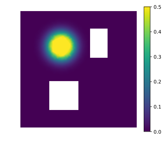
We consider a Gaussian prior for the parameter $m\sim\mathcal{N}(m_{\text{pr}},\mathcal{C}_{\text{pr}})$ with mean $m_{\text{pr}}$ and covariance operator $\mathcal{C}_{\text{pr}}=\mathcal{A}^{-2}$ , where the elliptic operator $\mathcal{A}=-\gamma\Delta+\delta I$ (with Laplacian $\Delta$ and identity $I$ ) is equipped with Robin boundary condition $\gamma\nabla m\cdot\mathbf{n}+\beta m$ on $\partial\mathcal{D}$ . Here $\gamma,\delta>0$ control the correlation length and variance of $m$ [24]. In our numerical test, we set $m_{\text{pr}}=0.25$ , $\gamma=1,\delta=8$ . We synthesize a “true” initial condition $m_{\text{true}}=\min(0.5,\exp(-100\left\lVert x-[0.35,0.7]\right\rVert^{2})$ as the contaminant source (fig. 1b). To solve the PDE model, we use an implicit Euler method for temporal discretization with $N_{t}$ time steps, and a finite element method for spatial discretization, resulting in a $d_{m}$ -dimensional discrete parameter $\mathbf{m}\sim\mathcal{N}(\mathbf{m}_{\text{pr}},\mathbf{\Gamma}_{\text{pr}})$ , with $\mathbf{m}_{\text{pr}},\mathbf{\Gamma}_{\text{pr}}$ denoting finite element discretizations of $m_{\text{pr}},\mathcal{C}_{\text{pr}}$ , respectively.

The solution of the PDE for $d_{m}=2023$ and $N_{t}=40$ at the observation time $T=0.8$ and $d$ candidate sensor locations are also shown in fig. 1c and fig. 1d, at which we observe the contaminant concentration $u$ . The linear map $\mathbf{F}$ is defined by the predicted data, i.e., the concentrations at the selected sensors. Finally, we take the QoI as an averaged contaminant concentration at time $t_{\text{pred}}$ within a distance $\delta=0.02$ from the boundaries of either the left, the right, or both buildings, with corresponding QoI maps denoted as $\mathbf{P}_{1},\mathbf{P}_{2},\mathbf{P}_{3}$ (see fig. 1c and fig. 1d).

4.2 Numerical results

We first consider the case of a small number of candidate sensors, for which we can use exhaustive search to find the optimal sensor combination and compare it with the sensors chosen by the standard and swapping greedy algorithms. Specifically, we use a grid of $d=9$ candidate locations $\{s_{i}\}_{i=0}^{9}$ ( $x_{i}\in\{0.2,0.55,0.8\}\times\{0.25,0.5,0.75\}$ ) as shown in (left) with the goal of choosing $r=2,3,4,5,6,7,8$ sensors for the QoI prediction time $t_{\text{pred}}=1.0$ . We compute the matrices $\mathbf{H}_{d}^{\rho}$ and $\Delta\mathbf{H}_{d}$ (of size $9\times 9$ ) without low-rank approximation since they are small.

(a)

\mathbf{P}_{1}

(b)

\mathbf{P}_{2}

(c)

\mathbf{P}_{3}

Figure 2: Approximate EIG

\hat{\Psi}^{\rho}

r

sensors chosen by the standard and swapping greedy algorithms, and the distribution of

\hat{\Psi}^{\rho}

at all possible combinations of

9

candidate sensors. The three plots are for the QoI maps

\mathbf{P}_{1},\mathbf{P}_{2}

, and

\mathbf{P}_{3}

We can see from fig. 2 that for QoI maps $\mathbf{P}_{1}$ and $\mathbf{P}_{2}$ , both greedy algorithms find the optimal design, while for $\mathbf{P}_{3}$ with $r=2,4$ , only swapping greedy finds the optimal design. Moreover, an increase in $r$ leads to diminishing returns, as the gain in information about the QoI from additional sensors saturates. We see that $\sim$ 3 sensors is sufficient for either building, whereas 5 is sufficient for both.

Next we consider the case of the 75 candidate sensors depicted in (right). Exhaustive search across all sensor combinations is not feasible in this case; instead, we compare the best EIG from $200$ random designs with those obtained by the greedy algorithms. We seek the $r$ optimal sensors, $r=5,10,15,20,25,30,40,50,60$ , from among the 75 candidates. Results are shown in fig. 3.

(a)

\mathbf{P}_{1}

(b)

\mathbf{P}_{2}

(c)

\mathbf{P}_{3}

Figure 3: Approximate EIG

\hat{\Psi}^{\rho}

for

r

out of 75 sensors, found by the standard and swapping greedy algorithms, compared with the distribution of

\hat{\Psi}^{\rho}

for 200 randomly-chosen sets from the

75

. The three plots are for the QoI maps

\mathbf{P}_{1},\mathbf{P}_{2}

and

\mathbf{P}_{3}

We see that both greedy algorithms find designs with larger EIG than all random choices. Moreover, for small $r$ , the swapping greedy algorithm finds better designs than the standard greedy. For large $r$ , both greedy algorithms can find designs with similar EIG. In fact, multiple designs with similar EIG become more likely with larger $r$ .

To demonstrate the reduction of computational cost achieved by the offline-online decomposition, we report the total number of EIG evaluations, the number of swapping loops, and the number of swaps of the swapping greedy algorithm (algorithm 1) in table 1 for $75$ candidate sensors with different target number of sensors. We see that the number of loops at convergence is mostly $3$ . We observe in the experiments that most of the swaps take place in the first loop, followed by a smaller number of swaps in the second loop resulting in slight sensor adjustments. There are no swaps in the last loop, which we require as a convergence criterion. As a result of the offline-online decomposition theorem 2, which relieves the (thousands of) EIG evaluations of expensive PDE solves once the low-rank approximation (28) is built, we achieve over 1000X speedup. This is because the PDE solves overwhelmingly dominate the overall cost, and because the offline decomposition is computed at a cost comparable to one direct EIG evaluation by (18).

Table 1: Number of swapping loops (#LOOPS), swaps (# SWAPS), and EIG evaluations (# EIG EVAL) for different numbers of

r

selected sensors out of 75 candidates. Results are reported for algorithm 1 for the goal

\mathbf{P}_{1}

$r$	$5$	$10$	$15$	$20$	$25$
#loops	$3$	$3$	$3$	$3$	$3$
#swaps	$41$	$73$	$124$	$164$	$190$
#EIG eval	$1050$	$1950$	$2700$	$3300$	$3750$
$r$	$30$	$40$	$50$	$60$
#loops	$2$	$3$	$3$	$3$
#swaps	$194$	$235$	$199$	$119$
#EIG eval	$2700$	$4200$	$3750$	$2700$

(a)

\mathbf{P}_{1}

t_{\text{pred}}=1.

(b)

\mathbf{P}_{2}

t_{\text{pred}}=1.

(c)

\mathbf{P}_{3}

t_{\text{pred}}=1.

(d)

\mathbf{P}_{1}

t_{\text{pred}}=2.

(e)

\mathbf{P}_{1}

t_{\text{pred}}=4.

(f)

\mathbf{P}_{1}

t_{\text{pred}}=8.

Figure 4: Sensor locations chosen by the swapping greedy algorithm for

10

out of

75

candidates for the parameter-to-QoI maps

\mathbf{P}_{1},\mathbf{P}_{2},\mathbf{P}_{3}

at time

t_{\text{pred}}=1

and also

\mathbf{P}_{1}

at time

t_{\text{pred}}=2,4,8

Figure 4 illustrates the effect of the goal of maximizing information gain for the QoIs from optimally placed sensors. Specifically, for the parameter-to-QoI maps $\mathbf{P}_{1},\mathbf{P}_{2},\mathbf{P}_{3}$ that quantify the average contaminant concentration at time $t_{\text{pred}}=1$ around left, right, and both blocks, the goal-oriented OED finds the sensors depicted in the first row. For $\mathbf{P}_{1}$ at longer prediction times $t_{\text{pred}}=1,2,4,8$ , we see in the bottom row of fig. 4 that the optimal sensors are no longer placed in the immediate vicinity of the building, but instead are increasingly dispersed to better detect the now more diffused field. Finally, the ability of GOOED to reduce the posterior variance in the initial condition field is depicted in fig. 5 for different goals $\mathbf{P}_{1},\mathbf{P}_{2},\mathbf{P}_{3}$ . Compared to a random design (lower right), the three optimal designs lead to lower variance surrounding regions of interest.

(a) optimal design for

\mathbf{P}_{1}

(b) optimal design for

\mathbf{P}_{2}

\mathbf{P}_{3}

(d) random design

Figure 5: Pointwise posterior variance of the parameter at optimal designs for goals

\mathbf{P}_{1}

\mathbf{P}_{2}

\mathbf{P}_{3}

, compared to a random design, for 10 sensors. The darker regions represent lower variance.

4.3 Scalability w.r.t. parameter and data dimensions

Here we demonstrate the fast decay of the eigenvalues of $\mathbf{H}_{d}^{\rho}$ and $\Delta\mathbf{H}_{d}$ with respect to the parameter and data dimensions, as exploited by the algorithms of section 3.3. For $\mathbf{H}_{d}^{\rho}$ defined in eq. 21, we have rank( $\mathbf{H}_{d}^{\rho}$ ) $\leq\min(p,d)$ with QoI dimension $p$ and data dimension $d$ . In practice, the QoI is often an averaged quantity with small $p$ , so the rank of $\mathbf{H}_{d}^{\rho}$ is also small. In our tests we have rank( $\mathbf{H}_{d}^{\rho}$ ) $=p=1$ . For $\Delta\mathbf{H}_{d}=\mathbf{H}_{d}-\mathbf{H}_{d}^{\rho}$ with $\mathbf{H}_{d}=\mathbf{F}_{d}\mathbf{\Gamma}_{\text{pr}}\mathbf{F}^{*}$ , the spectrum of $\Delta\mathbf{H}_{d}$ depends on that of $\mathbf{H}_{d}$ , which typically exhibits fast decay due to ill-posedness of inverse problems. As can be observed in the left plot of fig. 6, the eigenvalues of $\Delta\mathbf{H}_{d}$ decay very rapidly and independently of the parameter dimension, which implies that the required number of PDE solves is small and independent of the parameter dimension while achieving the same absolute accuracy of the approximate EIG by theorem 4. The right plot in fig. 6 also illustrates rapid decay of eigenvalues, as well as diminishing returns, with the increasing number of candidate sensors, suggesting that the number of PDE solves is asymptotically independent of the data dimension for the same relative accuracy of the approximate EIG. These plots suggest that $O(100)$ PDE solves are required to accurately capture the information gained about the parameter field and QoI from the data, regardless of the parameter or sensor dimensions, when using randomized SVD ( algorithm 2).

Figure 6: Decay of the eigenvalues of

\Delta\mathbf{H}_{d}

with the increasing parameter dimension (left) and data (candidate sensor locations) dimension (right).

5 Conclusions

We have developed a fast and scalable computational framework for goal-oriented linear Bayesian optimal experimental design governed by expensive models. Repeated fast evaluation of an (arbitrarily accurate) approximate EIG while avoiding model evaluations is made possible by an offline-online decomposition and low-rank approximation of certain operators informed by the parameter, data, and predictive goals of interest. Scalability, as measured by parameter- and data-dimension independence of the number of model evaluations, is achieved by carefully exploiting the GOOED problem’s intrinsic low dimensionality as manifested by the rapid spectral decay of several critical operators. To justify the low-rank approximation of these operators in computing the EIG, we proved an upper bound for the approximation error in terms of the operators’ truncated eigenvalues. Moreover, we proposed a new swapping greedy algorithm that is demonstrated to be more effective than the standard greedy algorithm in our experiments. Numerical experiments with optimal sensor placement for Bayesian inference of the initial condition of an advection–diffusion PDE demonstrated over 1000X speedups (measured in PDE solves). Future work includes extension to nonlinear Bayesian GOOED problems with nonlinear parameter-to-observable maps and nonlinear parameter-to-QoI maps.

Appendix A: Low-rank approximation

To compute the low-rank approximations of $\Delta\mathbf{H}_{d}$ and $\mathbf{H}_{d}^{\rho}$ as described in section 3.3, we present the randomized SVD algorithm for these two quantities. Recall the explicit forms of $\Delta\mathbf{H}_{d}$ and $\mathbf{H}_{d}^{\rho}$ as

\mathbf{H}^{\rho}_{d}=\mathbf{F}_{d}\mathbf{\Gamma}_{\text{pr}}\mathbf{P}^{*}\mathbf{\Sigma}_{\text{pr}}^{-1}\mathbf{P}\mathbf{\Gamma}_{\text{pr}}\mathbf{F}_{d}^{*},\Delta\mathbf{H}_{d}=\mathbf{F}_{d}\mathbf{\Gamma}_{\text{pr}}\mathbf{F}_{d}^{*}-\mathbf{F}_{d}\mathbf{\Gamma}_{\text{pr}}\mathbf{P}^{*}\mathbf{\Sigma}_{\text{pr}}^{-1}\mathbf{P}\mathbf{\Gamma}_{\text{pr}}\mathbf{F}_{d}^{*}.

(54)

Algorithm 2 Randomized SVD to compute

\mathbf{H}

with low rank

k

1: Generate i.i.d. Gaussian matrix

\bm{\Omega}\in\mathbb{R}^{d\times(k+p)}

with an oversampling parameter

p

very small (e.g.,

p=10

2: Compute

\bm{Y}=\mathbf{H}\bm{\Omega}.

3: Compute the QR factorization

\bm{Y}=\bm{Q}\bm{R}

satisfying

\bm{Q}^{T}\bm{Q}=\bm{I}

4: Compute

\bm{B}=\bm{Q}^{T}\mathbf{H}\bm{Q}

5: Solve an eigenvalue problem for

\bm{B}

such that

\bm{B}=\bm{Z}\bm{\Sigma}\bm{Z}^{T}

6: Form

U_{k}=\bm{Q}\bm{Z}[1:k]

and

\Sigma_{k}=\bm{\Sigma}[1:k,1:k]

We see that this is a matrix-free eigensolver. Steps 2 and 4 represent $\Delta\mathbf{H}_{d}$ action on $O(2(l+p))$ vectors and $\mathbf{H}_{d}^{\rho}$ action on $O(2(k+p))$ vectors. In terms of the total actions, it requires $2(2l+k+p)$ forward operator $\mathbf{F}$ and $2(l+k+p)$ of its adjoint $\mathbf{F}^{*}$ , $2(k+l+p)$ prediction operator $\mathbf{P}$ and its adjoint $\mathbf{P}^{*}$ .

For the contaminant problem given in section 4.1, the concentration field $u(x,t)$ is given by

\begin{split}u_{t}-k\Delta u+\bm{v}\cdot\nabla u&=0\text{ in }\mathcal{D}\times(0,T),\\ u(\cdot,0)&=m\text{ in }\mathcal{D},\\ k\nabla u\cdot\bm{n}&=0\text{ on }\partial\mathcal{D}\times(0,T),\end{split}

(55)

we can form the parameter-to-observable map $\mathbf{F}\mathbf{m}$ as the discretized value of $\mathcal{B}u(m)$ where $\mathcal{B}$ is the pointwise observation operator. The adjoint problem is a terminal value problem which can be solved backwards in time by the equation:

\begin{split}-p_{t}-\nabla\cdot(p\bm{v})-k\Delta p&=\mathcal{B}^{*}\mathbf{y}\text{ in }\mathcal{D}\times(0,T),\\ p(\cdot,T)&=0\text{ in }\mathcal{D},\\ (p\bm{v}+k\nabla p)\cdot\bm{n}&=0\text{ on }\partial\mathcal{D}\times(0,T).\end{split}

(56)

Then we can define the adjoint of the parameter-to-observable map $\mathbf{F}^{*}\mathbf{y}$ as the discretized value of $p(x,0)$ for any $\mathbf{y}$ .

References

[1] A. Alexanderian, P. J. Gloor, and O. Ghattas, On Bayesian A-and D-optimal experimental designs in infinite dimensions, Bayesian Analysis, 11 (2016), pp. 671–695, https://doi.org/10.1214/15-BA969.
[2] A. Alexanderian, N. Petra, G. Stadler, and O. Ghattas, A-optimal design of experiments for infinite-dimensional Bayesian linear inverse problems with regularized $\ell_{0}$ -sparsification, SIAM Journal on Scientific Computing, 36 (2014), pp. A2122–A2148, https://doi.org/10.1137/130933381.
[3] A. Alexanderian, N. Petra, G. Stadler, and O. Ghattas, A fast and scalable method for A-optimal design of experiments for infinite-dimensional Bayesian nonlinear inverse problems, SIAM Journal on Scientific Computing, 38 (2016), pp. A243–A272, https://doi.org/10.1137/140992564.
[4] A. Alexanderian, N. Petra, G. Stadler, and O. Ghattas, Mean-variance risk-averse optimal control of systems governed by PDEs with random parameter fields using quadratic approximations, SIAM/ASA Journal on Uncertainty Quantification, 5 (2017), pp. 1166–1192, https://doi.org/10.1137/16M106306X.
[5] A. Alexanderian and A. K. Saibaba, Efficient D-optimal design of experiments for infinite-dimensional Bayesian linear inverse problems, SIAM Journal on Scientific Computing, 40 (2018), pp. A2956–A2985, https://doi.org/10.1137/17M115712X.
[6] N. Alger, P. Chen, and O. Ghattas, Tensor train construction from tensor actions, with application to compression of large high order derivative tensors, SIAM Journal on Scientific Computing, 42 (2020), pp. A3516–A3539.
[7] I. Ambartsumyan, W. Boukaram, T. Bui-Thanh, O. Ghattas, D. Keyes, G. Stadler, G. Turkiyyah, and S. Zampini, Hierarchical matrix approximations of Hessians arising in inverse problems governed by PDEs, SIAM Journal on Scientific Computing, 42 (2020), pp. A3397–A3426.
[8] A. Attia, A. Alexanderian, and A. K. Saibaba, Goal-oriented optimal design of experiments for large-scale bayesian linear inverse problems, Inverse Problems, 34 (2018), p. 095009.
[9] T. Bakker, H. van Hoof, and M. Welling, Experimental design for MRI by greedy policy search, Advances in Neural Information Processing Systems, 33 (2020).
[10] O. Bashir, K. Willcox, O. Ghattas, B. van Bloemen Waanders, and J. Hill, Hessian-based model reduction for large-scale systems with initial condition inputs, International Journal for Numerical Methods in Engineering, 73 (2008), pp. 844–868.
[11] A. A. Bian, J. M. Buhmann, A. Krause, and S. Tschiatschek, Guarantees for greedy maximization of non-submodular functions with applications, in Proceedings of the 34th International Conference on Machine Learning-Volume 70, JMLR. org, 2017, pp. 498–507.
[12] C. Boutsidis, M. W. Mahoney, and P. Drineas, An improved approximation algorithm for the column subset selection problem, CoRR, abs/0812.4293 (2008), http://arxiv.org/abs/0812.4293, https://arxiv.org/abs/0812.4293.
[13] T. Bui-Thanh, C. Burstedde, O. Ghattas, J. Martin, G. Stadler, and L. C. Wilcox, Extreme-scale UQ for Bayesian inverse problems governed by PDEs, in SC12: Proceedings of the International Conference for High Performance Computing, Networking, Storage and Analysis, 2012.
[14] T. Bui-Thanh, O. Ghattas, J. Martin, and G. Stadler, A computational framework for infinite-dimensional Bayesian inverse problems Part I: The linearized case, with application to global seismic inversion, SIAM Journal on Scientific Computing, 35 (2013), pp. A2494–A2523, https://doi.org/10.1137/12089586X.
[15] K. Chaloner and I. Verdinelli, Bayesian experimental design: A review, Statistical Science, 10 (1995), pp. 273–304.
[16] P. Chen and O. Ghattas, Hessian-based sampling for high-dimensional model reduction, International Journal for Uncertainty Quantification, 9 (2019).
[17] P. Chen and O. Ghattas, Projected Stein variational gradient descent, in Advances in Neural Information Processing Systems, 2020.
[18] P. Chen, M. Haberman, and O. Ghattas, Optimal design of acoustic metamaterial cloaks under uncertainty, Journal of Computational Physics, 431 (2021), p. 110114.
[19] P. Chen, U. Villa, and O. Ghattas, Hessian-based adaptive sparse quadrature for infinite-dimensional Bayesian inverse problems, Computer Methods in Applied Mechanics and Engineering, 327 (2017), pp. 147–172, https://doi.org/10.1016/j.cma.2017.08.016.
[20] P. Chen, U. Villa, and O. Ghattas, Taylor approximation and variance reduction for PDE-constrained optimal control under uncertainty, Journal of Computational Physics, 385 (2019), pp. 163–186, https://arxiv.org/abs/1804.04301.
[21] P. Chen, K. Wu, J. Chen, T. O’Leary-Roseberry, and O. Ghattas, Projected Stein variational Newton: A fast and scalable Bayesian inference method in high dimensions, Advances in Neural Information Processing Systems, (2019).
[22] P. Chen, K. Wu, and O. Ghattas, Bayesian inference of heterogeneous epidemic models: Application to COVID-19 spread accounting for long-term care facilities, arXiv preprint arXiv:2011.01058, (2020).
[23] B. Crestel, A. Alexanderian, G. Stadler, and O. Ghattas, A-optimal encoding weights for nonlinear inverse problems, with application to the Helmholtz inverse problem, Inverse Problems, 33 (2017), p. 074008, http://iopscience.iop.org/10.1088/1361-6420/aa6d8e.
[24] Y. Daon and G. Stadler, Mitigating the influence of boundary conditions on covariance operators derived from elliptic PDEs, Inverse Problems and Imaging, 12 (2018), pp. 1083–1102, https://arxiv.org/abs/1610.05280.
[25] A. R. Ferrolino, J. E. C. Lope, and R. G. Mendoza, Optimal location of sensors for early detection of tsunami waves, in International Conference on Computational Science, Springer, 2020, pp. 562–575.
[26] P. H. Flath, L. C. Wilcox, V. Akçelik, J. Hill, B. van Bloemen Waanders, and O. Ghattas, Fast algorithms for Bayesian uncertainty quantification in large-scale linear inverse problems based on low-rank partial Hessian approximations, SIAM Journal on Scientific Computing, 33 (2011), pp. 407–432, https://doi.org/10.1137/090780717.
[27] A. Foster, M. Jankowiak, E. Bingham, P. Horsfall, Y. W. Teh, T. Rainforth, and N. Goodman, Variational Bayesian optimal experimental design, in Advances in Neural Information Processing Systems, H. Wallach, H. Larochelle, A. Beygelzimer, F. d'Alché-Buc, E. Fox, and R. Garnett, eds., vol. 32, Curran Associates, Inc., 2019, pp. 14036–14047, https://proceedings.neurips.cc/paper/2019/file/d55cbf210f175f4a37916eafe6c04f0d-Paper.pdf.
[28] N. Halko, P. G. Martinsson, and J. A. Tropp, Finding structure with randomness: Probabilistic algorithms for constructing approximate matrix decompositions, SIAM Review, 53 (2011), pp. 217–288.
[29] X. Huan and Y. M. Marzouk, Simulation-based optimal Bayesian experimental design for nonlinear systems, Journal of Computational Physics, 232 (2013), pp. 288–317, https://doi.org/http://dx.doi.org/10.1016/j.jcp.2012.08.013, http://www.sciencedirect.com/science/article/pii/S0021999112004597.
[30] X. Huan and Y. M. Marzouk, Gradient-based stochastic optimization methods in Bayesian experimental design, International Journal for Uncertainty Quantification, 4 (2014), pp. 479–510.
[31] X. Huan and Y. M. Marzouk, Sequential bayesian optimal experimental design via approximate dynamic programming, arXiv preprint arXiv:1604.08320, (2016).
[32] T. Isaac, N. Petra, G. Stadler, and O. Ghattas, Scalable and efficient algorithms for the propagation of uncertainty from data through inference to prediction for large-scale problems, with application to flow of the Antarctic ice sheet, Journal of Computational Physics, 296 (2015), pp. 348–368, https://doi.org/10.1016/j.jcp.2015.04.047.
[33] J. Jagalur-Mohan and Y. Marzouk, Batch greedy maximization of non-submodular functions: Guarantees and applications to experimental design, arXiv preprint arXiv:2006.04554, (2020).
[34] K. Kandasamy, W. Neiswanger, R. Zhang, A. Krishnamurthy, J. Schneider, and B. Poczos, Myopic posterior sampling for adaptive goal oriented design of experiments, in International Conference on Machine Learning, PMLR, 2019, pp. 3222–3232.
[35] S. Kleinegesse and M. U. Gutmann, Bayesian experimental design for implicit models by mutual information neural estimation, in International Conference on Machine Learning, PMLR, 2020, pp. 5316–5326.
[36] Q. Long, M. Scavino, R. Tempone, and S. Wang, Fast estimation of expected information gains for Bayesian experimental designs based on Laplace approximations, Computer Methods in Applied Mechanics and Engineering, 259 (2013), pp. 24–39.
[37] N. Loose and P. Heimbach, Leveraging uncertainty quantification to design ocean climate observing systems, Journal of Advances in Modeling Earth Systems, (2021), pp. 1–29.
[38] T. O’Leary-Roseberry, U. Villa, P. Chen, and O. Ghattas, Derivative-informed projected neural networks for high-dimensional parametric maps governed by PDEs, Computer Methods in Applied Mechanics and Engineering, 388 (2022), p. 114199.
[39] N. Petra, J. Martin, G. Stadler, and O. Ghattas, A computational framework for infinite-dimensional Bayesian inverse problems: Part II. Stochastic Newton MCMC with application to ice sheet flow inverse problems, SIAM Journal on Scientific Computing, 36 (2014), pp. A1525–A1555.
[40] C. Pozrikidis, An introduction to grids, graphs, and networks, Oxford University Press, 2014.
[41] A. K. Saibaba, A. Alexanderian, and I. C. Ipsen, Randomized matrix-free trace and log-determinant estimators, Numerische Mathematik, 137 (2017), pp. 353–395.
[42] A. Spantini, T. Cui, K. Willcox, L. Tenorio, and Y. M. Marzouk, Goal-oriented optimal approximations of Bayesian linear inverse problems, SIAM Journal on Scientific Computing, 39 (2017), pp. S167–S196.
[43] K. Wu, P. Chen, and O. Ghattas, A fast and scalable computational framework for large-scale and high-dimensional Bayesian optimal experimental design, arXiv preprint arXiv:2010.15196, (2020).
[44] M.-C. Yue, A matrix generalization of the hardy-littlewood-pólya rearrangement inequality and its applications, arXiv preprint arXiv:2006.08144, (2020).
[45] S. Zheng, D. Hayden, J. Pacheco, and J. W. Fisher III, Sequential Bayesian experimental design with variable cost structure, Advances in Neural Information Processing Systems, 33 (2020).

An efficient method for goal-oriented linear Bayesian optimal experimental design: Application to optimal sensor placement Thanks: Submitted to the editors DATE.

Abstract

keywords

Funding.

AMS

1 Introduction

2 Background

2.1 Linear Bayesian inverse problem

2.2 Bayesian optimal experimental design

2.2.1 Expected information gain

2.2.2 BOED for sensor placement

3 Goal-oriented optimal experimental design

3.1 Expected information gain for GOOED

Proposition 1.

3.2 Offline-online decomposition for EIG Ψρ\Psi^{\rho}

Theorem 2.

Proof.

Proposition 3.

3.3 Low-rank approximation

Theorem 4.

Proof.

Proposition 5.

Proposition 6.

Proposition 7.

Lemma 8.

Proof.

3.4 Swapping greedy optimization

4 Experiments

4.1 Model settings

4.2 Numerical results

4.3 Scalability w.r.t. parameter and data dimensions

5 Conclusions

Appendix A: Low-rank approximation

References

3.2 Offline-online decomposition for EIG $\Psi^{\rho}$