Online Graph Dictionary Learning

Cédric Vincent-Cuaz Affiliation: Univ.Côte d’Azur, Inria, CNRS, LJAD, Maasai, Nice, France Correspondence to: cedric.vincent-cuaz@inria.fr Titouan Vayer Affiliation: ENS de Lyon, LIP UMR 5668, Lyon, France Rémi Flamary Affiliation: Ecole Polytechnique, CMAP, UMR 7641, Palaiseau, France Marco Corneli Affiliation: Univ.Côte d’Azur, Inria, CNRS, LJAD, Maasai, Nice, France Affiliation: Univ.Côte d’Azur, Center of Modeling, Simulation & Interaction,
Nice, France Nicolas Courty Affiliation: Univ.Bretagne-Sud, CNRS, IRISA, Vannes, France

Abstract

Dictionary learning is a key tool for representation learning, that explains the data as linear combination of few basic elements. Yet, this analysis is not amenable in the context of graph learning, as graphs usually belong to different metric spaces. We fill this gap by proposing a new online Graph Dictionary Learning approach, which uses the Gromov Wasserstein divergence for the data fitting term. In our work, graphs are encoded through their nodes’ pairwise relations and modeled as convex combination of graph atoms, i.e. dictionary elements, estimated thanks to an online stochastic algorithm, which operates on a dataset of unregistered graphs with potentially different number of nodes. Our approach naturally extends to labeled graphs, and is completed by a novel upper bound that can be used as a fast approximation of Gromov Wasserstein in the embedding space. We provide numerical evidences showing the interest of our approach for unsupervised embedding of graph datasets and for online graph subspace estimation and tracking.

Keywords:

Machine Learning, ICML

1 Introduction

The question of how to build machine learning algorithms able to go beyond vectorial data and to learn from structured data such as graphs has been of great interest in the last decades. Notable applications can be found in molecule compounds (Kriege et al. 2018), brain connectivity (Ktena et al. 2017), social networks (Yanardag & Vishwanathan 2015), time series (Cuturi & Blondel 2018), trees (Day 1985) or images (Harchaoui & Bach 2007; Bronstein et al. 2017). Designing good representations for these data is challenging, as their nature is by essence non-vectorial, and requires dedicated modelling of their representing structures. Given sufficient data and labels, end-to-end approaches with neural networks have shown great promises in the last years (Wu et al. 2020). In this work, we focus on the unsupervised representation learning problem, where the entirety of the data might not be known beforehand, and is rather produced continuously by different sensors, and available through streams. In this setting, tackling the non-stationarity of the underlying generating process is challenging (Ditzler et al. 2015). Good examples can be found, for instance, in the context of dynamic functional connectivity (Heitmann & Breakspear 2018) or network science (Masuda & Lambiotte 2020). As opposed to recent approaches focusing on dynamically varying graphs in online or continuous learning (Yang et al. 2018; Vlaski et al. 2018; Wang et al. 2020), we rather suppose in this work that distinct graphs are made progressively available (Zambon et al. 2017; Grattarola et al. 2019). This setting is particularly challenging as the structure, the attributes or the number of nodes of each graph observed at a time step can differ from the previous ones. We propose to tackle this problem by learning a linear representation of graphs with online dictionary learning.

Dictionary Learning (DL)

Dictionary Learning (Mairal et al. 2009; Schmitz et al. 2018) is a field of unsupervised learning that aims at estimating a linear representation of the data, i.e. to learn a linear subspace defined by the span of a family of vectors, called atoms, which constitute a dictionary. These atoms are inferred from the input data by minimizing a reconstruction error. These representations have been notably used in statistical frameworks such as data clustering (Ng et al. 2002), recommendation systems (Bobadilla et al. 2013) or dimensionality reduction (Candès et al. 2011). While DL methods mainly focus on vectorial data,

it is of prime interest to investigate flexible and interpretable factorization models applicable to structured data. We also consider the dynamic or time varying version of the problem, where the data generating process may exhibit non-stationarity over time, yielding a problem of subspace change or tracking (see e.g. (Narayanamurthy & Vaswani 2018)), where one wants to monitor changes in the subspace best describing the data. In this work, we rely on optimal transport as a fidelity term to compare these structured data.

Optimal Transport for structured data

Optimal Transport (OT) theory provides a set of methods for comparing probability distributions, using, e.g. the well-known Wasserstein distance (Villani 2003). It has been notably used by the machine learning community in the context of distributional unsupervised learning (Arjovsky et al. 2017; Schmitz et al. 2018; Peyré & Cuturi 2019). Broadly speaking the interest of OT lies in its ability to provide correspondences, or relations, between sets of points. Consequently, it has recently garnered attention for learning tasks where the points are described by graphs/structured data (see e.g. (Nikolentzos et al. 2017; Maretic et al. 2019; Togninalli et al. 2019; Xu et al. 2019a; Vayer et al. 2019; Barbe et al. 2020)). One of the key ingredient in this case is to rely on the so called Gromov-Wasserstein (GW) distance (Mémoli 2011; Sturm 2012) which is an OT problem adapted to the scenario in which the supports of the probability distributions lie in different metric spaces. The GW distance is particularly suited for comparing relational data (Peyré et al. 2016; Solomon et al. 2016) and, in a graph context, is able to find the relations between the nodes of two graphs when their respective structure is encoded through the pairwise relationship between the nodes in the graph. GW has been further studied for weighted directed graphs in (Chowdhury & Mémoli 2019) and has been extended to labeled graphs thanks to the Fused Gromov-Wasserstein (FGW) distance in (Vayer et al. 2018). Note that OT divergences as losses for linear and non-linear DL over vectorial data have already been proposed in (Bonneel et al. 2016; Rolet et al. 2016; Schmitz et al. 2018) but the case of structured data remains quite unaddressed. A non-linear DL approach for graphs based on GW was proposed in (Xu 2020) but suffers from a lack of interpretability and high computational complexity (see discussions in Section 3). To the best of our knowledge, a linear counterpart does not exist for now.

Refer to caption — Figure 1: From a dataset of graphs with different number of nodes, our method builds a dictionary of graph atoms with an online procedure. It uses the Gromov-Wasserstein distance as data fitting term between a convex combination of the atoms and a pairwise relations representation for graphs from the dataset.

Contributions

In this paper we use OT distances between structured data to design a linear and online DL for undirected graphs. Our proposal is depicted in Figure 1. It consists in a new factorization model for undirected graphs optionally having node attributes relying on (F)GW distance as data fitting term. We propose an online stochastic algorithm to learn the dictionary which scales to large real-world data (Section 2.3), and uses extensively novel derivations of sub-gradients of the (F)GW distance (Section 2.4). An unmixing procedure projects the graph in an embedding space defined w.r.t. the dictionary (Section 2.2). Interestingly enough, we prove that the GW distance in this embedding is upper-bounded by a Mahalanobis distance over the space of unmixing weights, providing a reliable and fast approximation of GW (Section 2.1). Moreover, this approximation defines a proper kernel that can be efficiently used for clustering and classification of graphs datasets (sections 4.1-4.2). We empirically demonstrate the relevance of our approach for online subspace estimation and subspace tracking by designing streams of graphs over two datasets (Section 4.3).

Notations

The simplex of histograms with $N$ bins is $\Sigma_{N}:=\left\{\mathbf{h}\in\mathbb{R}^{+}_{N}|\sum_{i}h_{i}=1\right\}$ . Let denote $S_{N}({\mathbb{R}})$ the set of symmetric matrices in ${\mathbb{R}}^{N\times N}$ . The Euclidean norm is denoted as $\|.\|_{2}$ and $\langle.,.\rangle_{F}$ the Frobenius inner product. We denote the gradient of a function $f$ over ${\bm{x}}$ at ${\bm{y}}$ in a stochastic context by $\widetilde{\nabla}_{{\bm{x}}}f({\bm{y}})$ . The number nodes in a graph is called the order of the graph.

2 Online Graph Dictionary Learning

2.1 (Fused) Gromov-Wasserstein for graph similarity

A graph $G^{X}$ with $N^{X}$ nodes, can be regarded as a tuple $({\bm{C}}^{X},{\bf h}^{X})$ where ${\bm{C}}^{X}\in{\mathbb{R}}^{N^{X}\times N^{X}}$ is a matrix that encodes a notion of similarity between nodes and ${\bf h}^{X}\in\Sigma_{N^{X}}$ is a histogram, or equivalently a vector of weights which models the relative importance of the nodes within the graph. Without any prior knowledge uniform weights can be chosen so that ${\bf h}^{X}=\frac{1}{N^{X}}\mathbf{1}_{N^{X}}$ . The matrix ${\bm{C}}^{X}$ carries the neighbourhood information of the nodes and, depending on the context, it may designate the adjacency matrix, the Laplacian matrix (Maretic et al. 2019) or the matrix of the shortest-path distances between the nodes (Bavaud 2010). Let us now consider two graphs $G^{X}=({\bm{C}}^{X},{\bf h}^{X})$ and $G^{Y}=({\bm{C}}^{Y},{\bf h}^{Y})$ , of potentially different orders (i.e $N^{X}\neq N^{Y}$ ). The $GW_{2}$ distance between $G^{X}$ and $G^{Y}$ is defined as the result of the following optimization problem:

\min_{{\bm{T}}\in\mathcal{U}({\bm{h}}^{X},{\bm{h}}^{Y})}\sum_{ijkl}\left(C^{X}_{ij}-C^{Y}_{kl}\right)^{2}T_{ik}T_{jl}

(1)

where $\mathcal{U}({\bm{h}}^{X},{\bm{h}}^{Y}):=\{{\bm{T}}\in{\mathbb{R}}_{+}^{N^{X}\times N^{Y}}|{\bm{T}}\mathbf{1}_{N^{Y}}={\bm{h}}^{X},{\bm{T}}^{T}\mathbf{1}_{N^{X}}={\bm{h}}^{Y}\}$ is the set of couplings between ${\bm{h}}^{X},{\bm{h}}^{Y}$ . The optimal coupling ${\bm{T}}$ of the GW problem acts as a probabilistic matching of nodes which tends to associate pairs of nodes that have similar pairwise relations in ${\bm{C}}^{X}$ and ${\bm{C}}^{Y}$ , respectively. In the following we denote by $GW_{2}({\bm{C}}^{X},{\bm{C}}^{Y},{\bm{h}}^{X},{\bm{h}}^{Y})$ the optimal value of equation 1 or by $GW_{2}({\bm{C}}^{X},{\bm{C}}^{Y})$ when the weights are uniform.

The previous framework can be extended to graphs with node attributes (typically ${\mathbb{R}}^{d}$ vectors). In this case we use the Fused Gromov-Wasserstein distance (FGW) (Vayer et al. 2018; Vayer et al. 2019) instead of GW. More precisely, a labeled graph $G^{X}$ with $N^{X}$ nodes can be described this time as a tuple $G^{X}=({\bm{C}}^{X},{\bm{A}}^{X},{\bm{h}}^{X})$ where ${\bm{A}}^{X}\in{\mathbb{R}}^{N^{X}\times d}$ is the matrix of all features. Given two labeled graphs $G^{X}$ and $G^{Y}$ , FGW aims at finding an optimal coupling by minimizing an OT cost which is a trade-off of a Wasserstein cost between the features and a GW cost between the similarity matrices. For the sake of clarity, we detail our approach in the GW context and refer the reader to the supplementary material for its extension to FGW.

2.2 Linear embedding and GW unmixing

Linear modeling of graphs

We propose to model a graph as a weighted sum of pairwise relation matrices. More precisely, given a graph $G=({\bm{C}},{\bm{h}})$ and a dictionary $\{\overline{{\bm{C}}}_{s}\}_{s\in[S]}$ we want to find a linear representation $\sum_{s\in[S]}w_{s}\overline{{\bm{C}}}_{s}$ of the graph $G$ , as faithful as possible. The dictionary is made of pairwise relation matrices of graphs with order $N$ . Thus, each $\overline{{\bm{C}}}_{s}\in S_{N}({\mathbb{R}})$ is called an atom, and ${\bm{w}}=(w_{s})_{s\in[S]}\in\Sigma_{S}$ is referred as embedding and denotes the coordinate of the graph $G$ in the dictionary as illustrated in Fig.1. We rely on the GW distance to assess the quality of our linear approximation and propose to minimize it to estimate its optimal embedding. In addition to being interpretable thanks to its linearity, we also propose to promote sparsity in the weights ${\bm{w}}$ similarly to sparse coding (Chen et al. 2001). Finally note that, when the pairwise matrices ${\bm{C}}$ are adjacency matrices and the dictionary atoms have components in $[0,1]$ , the model $\sum_{s\in[S]}w_{s}\overline{{\bm{C}}}_{s}$ provides a matrix whose components can be interpreted as probabilities of connection between the nodes.

Gromov-Wasserstein unmixing

We first study the unmixing problem that consists in projecting a graph on the linear representation discussed above, i.e. estimate the optimal embedding ${\bm{w}}$ of a graph $G$ . The unmixing problem can be expressed as the minimization of the GW distance between the similarity matrix associated to the graph and its linear representation in the dictionary:

\displaystyle\min_{{\bm{w}}\in\Sigma_{S}}\quad GW^{2}_{2}\left({\bm{C}},\sum_{s\in[S]}w_{s}\overline{{\bm{C}}}_{s}\right)-\lambda\|{\bm{w}}\|^{2}_{2}

(2)

Algorithm 1 BCD for unmixing problem 46

1: Initialize

{\bm{w}}=\frac{1}{S}\mathbf{1}_{S}

2: repeat

3: Compute OT matrix

{\bm{T}}

GW_{2}^{2}({\bm{C}},\sum_{s}w_{s}\overline{{\bm{C}}}_{s})

, with CG algorithm (Vayer et al. 2018, Alg.1 & 2).

4: Compute the optimal

{\bm{w}}

solving equation 46 for a fixed

{\bm{T}}

with CG algorithm.

5: until convergence

The BCD (Alg.3) works by alternatively updating the OT matrix of the GW distance and the embeddings ${\bm{w}}$ . When ${\bm{w}}$ is fixed the problem is a classical GW which is a non-convex quadratic program. We solve it using a Conditional Gradient (CG) algorithm (Jaggi 2013) based on (Vayer et al. 2019). Note that the use of the exact GW instead of a regularized proxy allowed us to keep a sparse OT matrix as well as to preserve “high frequency” components of the graph, as opposed to regularized versions of GW (Peyré et al. 2016; Solomon et al. 2016; Xu et al. 2019b) that promotes dense OT matrices and leads to smoothed/averaged pairwise matrices. For a fixed OT matrix ${\bm{T}}$ , the problem of finding ${\bm{w}}$ is a non-convex quadratic program and can also be tackled with a CG algorithm. Note that for non-convex problems the CG algorithm is known to converge to a local stationary point (Lacoste-Julien 2016). In practice, we observed a typical convergence of the CGs in a few tens of iterations. The BCD itself converges in less than 10 iterations.

Fast upper bound for GW

Interestingly, when two graphs belong to the linear subspace defined by our dictionary, there exists a proxy of the GW distance using a dedicated Mahalanobis distance as described in the next propositon:

Proposition 1

For two embedded graphs with embeddings ${\bm{w}}^{(1)}$ and ${\bm{w}}^{(2)}$ , assuming they share the same weights ${\bm{h}}$ , the following inequality holds

\displaystyle GW_{2}\left(\sum_{s\in[S]}w^{(1)}_{s}\overline{{\bm{C}}}_{s},\sum_{s\in[S]}w^{(2)}_{s}\overline{{\bm{C}}}_{s}\right)\leq\|{\bm{w}}^{(1)}-{\bm{w}}^{(2)}\|_{\bm{M}}

(3)

where $M_{pq}=\langle{\bm{D}}_{{\bm{h}}}\overline{{\bm{C}}}_{p},\overline{{\bm{C}}}_{q}{\bm{D}}_{{\bm{h}}}\rangle_{F}$ and ${\bm{D}}_{\bm{h}}=diag({\bm{h}})$ . ${\bm{M}}$ is a positive semi-definite matrix hence engenders a Mahalanobis distance between embeddings.

As detailed in the supplementary material, this upper bound is obtained by considering the GW cost between the linear models calculated using the admissible coupling ${\bm{D}}_{{\bm{h}}}$ . The latter coupling assumes that both graph representations are aligned and therefore is a priori suboptimal. As such, this bound is not tight in general. However, when the embeddings are close, the optimal coupling matrix should be close to ${\bm{D}}_{{\bm{h}}}$ so that Proposition 3 provides a reasonable proxy to the GW distance into our embedding space. In practice, this upper bound can be used to compute efficiently pairwise kernel matrices or to do retrieval of closest samples (see numerical experiments).

2.3 Dictionary learning and online algorithm

Assume now that the dictionary $\{\overline{{\bm{C}}}_{s}\}_{s\in[S]}$ is not known and has to be estimated from the data. We define a dataset of $K$ graphs $\left\{G^{(k)}:({\bm{C}}^{(k)},{\bm{h}}^{(k)})\right\}_{k\in[K]}$ . Recall that each graph $G^{(k)}$ of order $N^{(k)}$ is summarized by its pairwise relation matrix ${\bm{C}}^{(k)}\in S_{N^{(k)}}({\mathbb{R}})$ and weights ${\bm{h}}^{(k)}\in\Sigma_{N^{(k)}}$ over nodes, as described in Section 2.1. The DL problem, that aims at estimating the optimal dictionary for a given dataset can be expressed as:

\displaystyle\min_{\begin{smallmatrix}\{{\bm{w}}^{(k)}\}_{k\in[K]}\\ \{\overline{{\bm{C}}}_{s}\}_{s\in[S]}\end{smallmatrix}}

\displaystyle\sum_{k=1}^{K}GW^{2}_{2}\left({\bm{C}}^{(k)},\sum_{s\in[S]}w^{(k)}_{s}\overline{{\bm{C}}}_{s}\right)-\lambda\|{\bm{w}}^{(k)}\|^{2}_{2}

(4)

where ${\bm{w}}^{(k)}\in\Sigma_{S},\overline{{\bm{C}}}_{s}\in S_{N}({\mathbb{R}})$ . Note that the optimization problem above is a classical sparsity promoting dictionary learning on a linear subspace but with the important novelty that the reconstruction error is computed with the GW distance. This allows us to learn a graphs subspace of fixed order $N$ using a dataset of graphs with various orders. The sum over the errors in equation 52 can be seen as an expectation and we propose to devise an online strategy to optimize the problem similarly to the online DL proposed in (Mairal et al. 2009). The main idea is to update the dictionary $\{\overline{{\bm{C}}}_{s}\}_{s}$ with a stochastic estimation of the gradients on few dataset graphs (minibatch). At each stochastic update the unmixing problems are solved independently for each graph of the minibatch using a fixed dictionary $\{\overline{{\bm{C}}}_{s}\}_{s}$ , using the procedure described in Section 2.2. Then one can compute a gradient of the loss on the minibatch w.r.t $\{\overline{{\bm{C}}}_{s}\}_{s}$ and proceed to a projected gradient step. The stochastic update of the proposed algorithm is detailed in Alg.5. Note that it can be used on a finite dataset with possibly several epochs on the whole dataset or online in the presence of streaming graphs. We provide an example of such subspace tracking in Section 4.3. We will refer to our approach as GDL in the rest of the paper.

Algorithm 2 GDL: stochastic update of atoms

\{\overline{{\bm{C}}}_{s}\}_{s\in[S]}

1: Sample a minibatch of graphs

\mathcal{B}:=\{{\bm{C}}^{(k)}\}_{k\in\mathcal{B}}

2: Compute optimal

\{({\bm{w}}^{(k)},{\bm{T}}^{(k)})\}_{k\in[B]}

by solving B independent unmixing problems with Alg.3.

3: Projected gradient step with estimated gradients

\widetilde{\nabla}_{\overline{{\bm{C}}}_{s}}

(equation in supplementary),

\forall s\in[S]

\overline{{\bm{C}}}_{s}\leftarrow Proj_{S_{N}({\mathbb{R}})}(\overline{{\bm{C}}}_{s}-\eta_{C}\widetilde{\nabla}_{\overline{{\bm{C}}}_{s}})

(5)

Numerical complexity

The numerical complexity of GDL depends on the complexity of each update. The main computational bottleneck is the unmixing procedure that relies on multiple resolution of GW problems. The complexity of solving a GW with the CG algorithm between two graphs of order $N$ and $M$ and computing its gradient is dominated by $\mathcal{O}\left(N^{2}M+M^{2}N\right)$ operations (Peyré et al. 2016; Vayer et al. 2018). Thus given dictionary atoms of order $N$ , the worst case complexity can be only quadratic in the highest graph order in the dataset. For instance, estimating embedding on dataset IMDB-M (see Section 4.2) over 12 atoms takes on average $44$ ms per graph (on processor i9-9900K CPU 3.60GHz). We refer the reader to the supplementary for more details. Note that in addition to scale well to large datasets thanks to the stochastic optimization, our method also leads to important speedups when using the representations as input feature for other ML tasks. For instance, we can use the upper bound in equation 11 to compute efficiently kernels between graphs instead of computing all pairwise GW distances.

GDL on labeled graphs

We can also define the same DL procedure for labeled graphs using the FGW distance. The unmixing part defined in equation 46 can be adapted by considering a linear embedding of the similarity matrix and of the feature matrix parametrized by the same ${\bm{w}}$ . From an optimization perspective, finding the optimal coupling of FGW can be achieved using a CG procedure so that Alg.5 extends naturally to the FGW case. Note also that the upper bound of Proposition 3 can be generalized to this setting. This discussion is detailed in supplementary material.

2.4 Learning the graph structure and distribution

Recent researches have studied the use of potentially more general distributions ${\bm{h}}$ on the nodes of graphs than the naive uniform ones commonly used. (Xu et al. 2019a) empirically explored the use of distributions induced by degrees, such as parameterized power laws, $h_{i}=\frac{p_{i}}{\sum_{i}p_{i}}$ , where $p_{i}=(deg(x_{i})+a)^{b}$ with $a\in{\mathbb{R}}_{+}$ and $b\in[0,1]$ . They demonstrated the interest of this approach but also highlighted how hard it is to calibrate, which advocates for learning these distributions. With this motivation, we extend our GDL model defined in equation 52 and propose to learn atoms of the form $\{\overline{{\bm{C}}}_{s},\overline{{\bm{h}}}_{s}\}_{s\in[S]}$ . In this setting we have two independent dictionaries modeling the relative importance of the nodes with $\overline{{\bm{h}}}_{s}\in\Sigma_{N}$ , and their pairwise relations through $\overline{{\bm{C}}}_{s}$ . This dictionary learning problem reads:

	$\displaystyle\min_{\begin{subarray}{c}\{({\bm{w}}^{(k)},{\bm{v}}^{(k)})\}_{k\in[K]}\\ \{(\overline{{\bm{C}}}_{s},\overline{{\bm{h}}}_{s})\}_{s\in[S]}\end{subarray}}\sum_{k=1}^{K}$	$\displaystyle GW^{2}_{2}\left({\bm{C}}^{(k)},\widetilde{{\bm{C}}}({\bm{w}}^{(k)}),{\bm{h}}^{(k)},\widetilde{{\bm{h}}}({\bm{v}}^{(k)})\right)$
		$\displaystyle-\lambda\\|{\bm{w}}^{(k)}\\|^{2}_{2}-\mu\\|{\bm{v}}^{(k)}\\|^{2}_{2}$		(6)

where ${\bm{w}}^{(k)},{\bm{v}}^{(k)}\in\Sigma_{S}$ are the structure and distribution embeddings and the linear models are defined as:

\forall k,\ \widetilde{{\bm{h}}}({\bm{v}}^{(k)})=\sum_{s}v^{(k)}_{s}\overline{{\bm{h}}}_{s},\quad\widetilde{{\bm{C}}}({\bm{w}}^{(k)})=\sum_{s}w^{(k)}_{s}\overline{{\bm{C}}}_{s}

Here we exploit fully the GW formalism by estimating simultaneously the graph distribution $\widetilde{{\bm{h}}}$ and its geometric structure $\widetilde{{\bm{C}}}$ . Optimization problem 64 can be solved by an adaptation of stochastic Algorithm 5. We estimate the structure/node weights unmixings $({\bm{w}}^{(k)},{\bm{v}}^{(k)})$ over a minibatch of graphs with a BCD (see Section 2.3). Then we perform simultaneously a projected gradient step update of $\{\overline{{\bm{C}}}_{s}\}_{s}$ and $\{\overline{{\bm{h}}}_{s}\}_{s}$ . More details are given in the supplementary.

The optimization procedure above requires to have access to a gradient for the GW distance w.r.t. the weights. To the best of our knowledge no theoretical results exists in the literature for finding such gradients. We provide below a simple way to compute a subgradient for GW weights from subgradients of the well-known Wasserstein distance:

Proposition 2

Let $({\bm{C}}^{1},{\bm{h}}^{1})$ and $({\bm{C}}^{2},{\bm{h}}^{2})$ be two graphs. Let ${\bm{T}}^{*}$ be an optimal coupling of the GW problem between $({\bm{C}}^{1},{\bm{h}}^{1}),({\bm{C}}^{2},{\bm{h}}^{2})$ . We define the following cost matrix ${\bm{M}}({\bm{T}}^{*}):=\left(\sum_{kl}(C^{1}_{ik}-C^{2}_{jl})^{2}T^{*}_{kl}\right)_{ij}$ . Let $\bm{\alpha}^{*}({\bm{T}}^{*}),\bm{\beta}^{*}({\bm{T}}^{*})$ be the dual variables of the following linear OT problem:

\min_{{\bm{T}}\in\mathcal{U}({\bm{h}}^{1},{\bm{h}}^{2})}\langle{\bm{M}}({\bm{T}}^{*}),{\bm{T}}\rangle_{F}

(7)

Then $\bm{\alpha}^{*}({\bm{T}}^{*})$ (resp $\bm{\beta}^{*}({\bm{T}}^{*})$ ) is a subgradient of the function $GW_{2}^{2}({\bm{C}}^{1},{\bm{C}}^{2},\ \mathchoice{\mathbin{\vbox{\hbox{\scalebox{.5}{$\displaystyle\bullet$}}}}}{\mathbin{\vbox{\hbox{\scalebox{.5}{$\textstyle\bullet$}}}}}{\mathbin{\vbox{\hbox{\scalebox{.5}{$\scriptstyle\bullet$}}}}}{\mathbin{\vbox{\hbox{\scalebox{.5}{$\scriptscriptstyle\bullet$}}}}}\ ,{\bm{h}}^{2})$ (resp $GW_{2}^{2}({\bm{C}}^{1},{\bm{C}}^{2},{\bm{h}}^{1},\ \mathchoice{\mathbin{\vbox{\hbox{\scalebox{.5}{$\displaystyle\bullet$}}}}}{\mathbin{\vbox{\hbox{\scalebox{.5}{$\textstyle\bullet$}}}}}{\mathbin{\vbox{\hbox{\scalebox{.5}{$\scriptstyle\bullet$}}}}}{\mathbin{\vbox{\hbox{\scalebox{.5}{$\scriptscriptstyle\bullet$}}}}}\ )$ ).

The proposition above shows that the subgradient of GW w.r.t. the weights can be found by solving a linear OT problem which corresponds to a Wasserstein distance. The ground cost ${\bm{M}}({\bm{T}}^{*})$ of this Wasserstein is moreover the gradient (w.r.t. the couplings) of the optimal GW loss. Note that in practice the GW problem is solved with a CG algorithm which already requires to solve this linear OT problem at each iteration. In this way, after convergence, the gradient w.r.t. the weights can be extracted for free from the last iteration of the CG algorithm. The proof of proposition 2 is given in the supplementary material.

3 Related work and discussion

In this section we discuss the relation of our GDL framework with existing approaches designed to handle graph data. We first focus on existing contributions for graph representation in machine learning applications. Then, we discuss in more details the existing non-linear graph dictionary learning approach of (Xu 2020).

Graph representation learning

Processing of graph data in machine learning applications have traditionally been handled using implicit representations such as with graph kernels (Shervashidze et al. 2009; Vishwanathan et al. 2010). Recent results have shown the interest of using OT based distances to measure graph similarities and to design new kernels (Vayer et al. 2019; Maretic et al. 2019; Chowdhury & Needham 2020). However, one limit of kernel methods is that the representation of the graph is fixed a priori and cannot be adapted to specific datasets. On the other hand, Geometric deep learning approaches (Bronstein et al. 2017) attempt to learn the representation for structured data by means of deep learning (Scarselli et al. 2008; Perozzi et al. 2014; Niepert et al. 2016). Graph Neural Networks (Wu et al. 2020) have shown impressive performance for end-to-end supervised learning problems. Note that both kernel methods and many deep learning based representations for graphs suffer from the fundamental pre-image problem, that prevents recovering actual graph objects from the embeddings. Our proposed GDL aims at overcoming such a limit relying on an unmixing procedure that not only provides a simple vectorial representation on the dictionary but also allows a direct reconstruction of interpretable graphs (as illustrated in the experiments). A recent contribution potentially overcoming the pre-image problem is Grattarola et al. 2019. In that paper, a variational autoencoder is indeed trained to embed the observed graphs into a constant curvature Riemannian manifold. The aim of that paper is to represent the graph data into a space where the statistical tests for change detection are easier. We look instead for a latent representation of the graphs that remains as interpretable as possible. As a side note, we point out that our GDL embeddings might be used as input for the statistical tests developed by (Zambon et al. 2017; Zambon et al. 2019) to detect stationarity changes in the stochastic process generating the observed graphs (see for instance Figure 6) .

Non-linear GW dictionary learning of graphs

In a recent work, (Xu 2020) proposed a non-linear factorization of graphs using a regularized version of GW barycenters (Peyré et al. 2016) and denoted it as Gromov-Wasserstein Factorization (GWF). Authors propose to learn a dictionary $\{\overline{{\bm{C}}_{s}}\}_{s\in[S]}$ by minimizing over $\{\overline{{\bm{C}}}_{s}\}_{s\in[S]}$ and $\{{\bm{w}}^{(k)}\}_{k\in[K]}$ the quantity $\sum_{k=1}^{K}GW_{2}^{2}(\widetilde{{\bm{B}}}({\bm{w}}^{(k)};\{\overline{{\bm{C}}}_{s}\}_{s}),{\bm{C}}^{(k)})$ where $\widetilde{{\bm{B}}}({\bm{w}}^{(k)};\{\overline{{\bm{C}}}_{s}\}_{s})\in\arg\min_{{\bm{B}}}\sum_{s}w^{(k)}_{s}GW_{2}^{2}({\bm{B}},\overline{{\bm{C}}}_{s})$ is a GW barycenter. The main difference between GDL and this work lies in the linear representation of the approximated graph that we adopt whereas (Xu 2020) relies on the highly non-linear Gromov barycenter. As a consequence, the unmixing requires solving a complex bi-level optimization problem that is computationally expensive. Similarly, reconstructing a graph from this embedding requires again the resolution of a GW barycenter, whereas our linear reconstruction process is immediate. In Section 4, we show that our GDL representation technique compares favorably to GWF, both in terms of numerical complexity and performance.

4 Numerical experiments

This section aims at illustrating the behavior of the approaches introduced so far for both clustering (Sections 4.1-4.2) and online subspace tracking (Section 4.3).

Implementation details

The base OT solvers that are used in the algorithms rely on the POT toolbox (Flamary & Courty 2017). For our experiments, we considered the Adam algorithm (Kingma & Ba 2014) as an adaptive strategy for the update of the atoms with a fixed dataset, but used SGD with constant step size for the online experiments in Section 4.3. The code is available at https://github.com/cedricvincentcuaz/GDL.

4.1 GDL on simulated datasets

The GDL approach discussed in this section refers to equation 52. First we illustrate it on datasets simulated according to the well understood Stochastic Block Model (Holland et al. 1983; Wang & Wong 1987, SBM,) and show that we can recover embeddings and dictionary atoms corresponding to the generative structure.

Datasets description

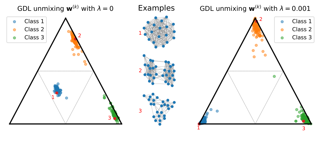
We consider two datasets of graphs, generated according to SBM, with various orders, randomly sampled in $\{10,15,...,60\}$ . The first scenario ( $D_{1}$ ) adopts three different generative structures (also referred to as classes): dense (no clusters), two clusters and three clusters (see Figures 2). Nodes are assigned to clusters into equal proportions. For each generative structure 100 graphs are sampled. The second scenario $(D_{2})$ considers the generative structure with two clusters, but with varying proportions of nodes for each block (see top of Figure 3), 150 graphs are simulated accordingly. In both scenarios we fix $p=0.1$ as the probability of inter-cluster connectivity and $1-p$ as the probability of intra-cluster connectivity. We consider adjacency matrices for representing the structures of the graphs in the datasets and uniform weights on the nodes.

Results and interpretation

First we learn on dataset $D_{1}$ a dictionary of 3 atoms of order 6. The unmixing coefficients for the samples in $D_{1}$ are reported in Fig. 2. On the left, we see that the coefficients are not sparse on the simplex but the samples are clearly well clustered and graphs sharing the same class (i.e. color) are well separated. When adding sparsity promoting regularization (right part of the figure) the different classes are clustered on the corners of the simplex, thus suggesting that regularization leads to a more discriminant representation. The estimated atoms for the regularized GDL are reported on the top of Fig. 1 as both matrices $\overline{{\bm{C}}}_{s}$ and their corresponding graphs. As it can be seen, the different SBM structures in $D_{1}$ are recovered. Next we estimate on $D_{2}$ a dictionary with 2 atoms of order 12. The interpolation between the two estimated atoms for some samples is reported in Fig. 3. As it can be seen, $D_{2}$ can be modeled as a one dimensional manifold where the proportion of nodes in each block changes continuously. We stress that the grey links on the bottom of Figure 3 correspond to the entries of the reconstructed adjacency matrices. Those entries are in $[0,1]$ , thus encoding a probability of connection (see Section 2.2). The darker the link, the higher the probability of interaction between the corresponding nodes. The possibility of generating random graphs using these probabilities opens the door to future researches.

We evaluate in Fig. 4 the quality of the Mahalanobis upper bound in equation 11 as a proxy for the GW distance on $D_{1}$ . On the left, one can see that the linear model allows us to recover the true GW distances between graphs most of the time. Exceptions occur for samples in the same class (i.e. ”near” to each other in terms of GW distance). The right part of the figure shows that the correlation between the Mahalanobis upper bound (cf. Proposition 3) and the GW distance between the embedded graphs is nearly perfect (0.999). This proves that our proposed upper bound provides a nice approximation of the GW distance between the input graphs, with a correlation of 0.96 (middle of the figure), at a much lower computational cost.

4.2 GDL on real data for clustering and classification

We now show how our unsupervised GDL procedure can be used to find meaningful representations for well-known graph classification datasets. The knowledge of the classes will be employed as a ground truth to validate our estimated embeddings in clustering tasks. For the sake of completeness, in supplementary material we also report the supervised classification accuracies of some recent supervised graph classification methods (e.g. GNN, kernel methods) showing that our DL and embedding is also competitive for classification.

Datasets and methods

We considered well-known benchmark datasets divided into three categories: i) IMDB-B and IMDB-M (Yanardag & Vishwanathan 2015) gather graphs without node attributes derived from social networks; ii) graphs with discrete attributes representing chemical compounds from MUTAG (Debnath et al. 1991) and cuneiform signs from PTC-MR (Krichene et al. 2015); iii) graphs with real vectors as attributes, namely BZR, COX2 (Sutherland et al. 2003) and PROTEINS, ENZYMES (Borgwardt & Kriegel 2005). We benchmarked our models for clustering tasks with the following state-of-the-art OT models: i) GWF (Xu 2020), using the proximal point algorithm detailed in that paper and exploring two configurations, i.e. with either fixed atom order (GWF-f) or random atom order (GWF-r, default for the method); ii) GW k-means (GW-k) which is a k-means using GW distances and GW barycenter (Peyré et al. 2016); iii) Spectral Clustering (SC) of (Shi & Malik 2000; Stella & Shi 2003) applied to the pairwise GW distance matrices or the pairwise FGW distance matrices for graphs with attributes. We complete these clustering evaluations with an ablation study of the effect of the negative quadratic regularization proposed with our models. As introduced in equation 52, this regularization is parameterized by $\lambda$ , so in this specific context we will distinguish GDL ( $\lambda=0$ ) from $\text{GDL}_{\lambda}$ ( $\lambda>0$ ).

Table 1: Clustering: Rand Index computed for benchmarked approaches on real datasets.

	NO ATTRIBUTE		DISCRETE ATTRIBUTES		REAL ATTRIBUTES
MODELS	IMDB-B	IMDB-M	MUTAG	PTC-MR	BZR	COX2	ENZYMES	PROTEIN
GDL (ours)	51.32(0.30)	55.08(0.28)	70.02(0.29)	51.53(0.36)	62.59(1.68)	58.39(0.52)	66.97(0.93)	60.22(0.30)
$\text{GDL}_{\lambda}$ (ours)	$\mathbf{51.64(0.59)}$	55.41(0.20)	$\mathbf{70.89(0.11)}$	$\mathbf{51.90(0.54)}$	$\mathbf{66.42(1.96)}$	$\mathbf{59.48(0.68)}$	66.79(1.12)	$\mathbf{60.49(0.71)}$
GWF-r	51.24 (0.02)	$\mathbf{55.54(0.03)}$	68.83(1.47)	51.44(0.52)	52.42(2.48)	56.84(0.41)	$\mathbf{72.13(0.19)}$	59.96(0.09)
GWF-f	50.47(0.34)	54.01(0.37)	58.96(1.91)	50.87(0.79)	51.65(2.96)	52.86(0.53)	71.64(0.31)	58.89(0.39)
GW-k	50.32(0.02)	53.65(0.07)	57.56(1.50)	50.44(0.35)	56.72(0.50)	52.48(0.12)	66.33(1.42)	50.08(0.01)
SC	50.11(0.10)	54.40(9.45)	50.82(2.71)	50.45(0.31)	42.73(7.06)	41.32(6.07)	70.74(10.60)	49.92(1.23)

Experimental settings

For the datasets with attributes involving FGW, we tested 15 values of the trade-off parameter $\alpha$ via a logspace search in $(0,0.5)$ and symmetrically $(0.5,1)$ and select the one minimizing our objectives. For our GDL methods as well as for GWF, a first step consists into learning the atoms. A variable number of $S=\beta k$ atoms is tested, where $k$ denotes the number of classes and $\beta\in\{2,4,6,8\}$ , with a uniform number of atoms per class. When the order $N$ of each atom is fixed, for GDL and GWF-f, it is set to the median order in the dataset. The atoms are initialized by randomly sampling graphs from the dataset with corresponding order. We tested 4 regularization coefficients for both methods.

The embeddings ${\bm{w}}$ are then computed and used as input for a k-means algorithm. However, whereas a standard Euclidean distance is used to implement k-means over the GWFs embeddings, we use the Mahalanobis distance from Proposition 3 for the k-means clustering of the GDLs embeddings. Unlike GDL and GWF, GW-k and SC do not require any embedding learning step. Indeed, GW-k directly computes (a GW) k-means over the input graphs and SC is applied to the GW distance matrix obtained from the input graphs. The cluster assignments are assessed by means of Rand Index (Rand 1971, RI,), computed between the true class assignment (known) and the one estimated by the different methods. For each parameter configuration (number of atoms, number of nodes and regularization parameter) we run each experiment five times, independently, with different random initializations. The mean RI was computed over the random initializations and the dictionary configuration leading to the highest RI was finally retained.

Results and interpretation

Clustering results can be seen in Table 1. The mean RI and its standard deviation are reported for each dataset and method. Our model outperforms or is at least comparable to the state-of-the-art OT based approaches for most of the datasets. Results show that the negative quadratic regularization proposed with our models brings additional gains in performance. Note that for this benchmark, we considered a fixed batch size for learning our models on labeled graphs, which turned out to be a limitation for the dataset ENZYMES. Indeed, comparable conclusions regarding our models performance have been observed by setting a higher batch size for this latter dataset and are reported in the supplementary material. This might be due to both a high number of heterogeneous classes and a high structural diversity of labeled graphs inside and among classes.

We illustrate in Fig. 5 the interest of the extension of GDL with estimated weights for IMDB-M dataset. We can see in the center-left part of the figure that, without estimating the weights, GDL can experience difficulties producing a model that preserves the global structure of the graph because of the uniform weights on the nodes. In opposition, simultaneously estimating the weights brings a more representative modeling (in the GW sense), as illustrated in the centred-right columns. The weights estimation can re-balance and even discard non relevant nodes, in the vein of attention mechanisms. We report in the supplementary material a companion study for clustering tasks which further supports our extension concerning the learning of node weights.

Figure 5: Modeling of two real life graphs from IMDB-M with our GDL approaches with 8 atoms of order 10. (left) original graphs from the dataset, (center left) linear model for GDL with uniform weights as in equation 52, (center right) linear model for GDL with estimated weights as in equation 64 and (right) different

\overline{{\bm{h}}}_{s}

on the estimated structure.

4.3 Online graph subspace estimation and change detection

Finally we provide experiments for online graph subspace estimation on simulated and real life datasets. We show that our approach can be used for subspace tracking of graphs as well as for change point detection of subspaces.

Datasets and experiments

In this section we considered two new large graph classification datasets: TWITCH-EGOS (Rozemberczki et al. 2020) containing social graphs without attributes belonging to 2 classes and TRIANGLES (Knyazev et al. 2019) that is a simulated dataset of labeled graphs with 10 classes. Here we investigate how our approach fits to online data, i.e. in the presence of a stream of graphs. The experiments are designed with different time segments where each segment streams graphs belonging to the same classes (or group of classes). The aim is to see if the method learns the current stream and detects or adapts to abrupt changes in the stream. For TWITCH-EGOS, we first streamed all graphs of a class (A), then graphs of the other class (B), both counting more than 60.000 graphs. All these graphs consist in a unique high-frequency (a hub structure) with sparse connections between non-central nodes (sparser for class B). For TRIANGLES, the stream follows the three groups A,B and C, with 10,000 graphs each, where the labels associated with each group are: $A=\{4,5,6,7\}$ , $B=\{8,9,10\}$ and $C=\{1,2,3\}$ .

Results and discussion

The online (F)GW losses and a running mean of these losses are reported for each dataset on the left part of Fig. 6. One the right part of the Figure, we report the average losses computed on several datasets containing data from each stream at some time instant along the iterations. First, the online learning for both datasets can be seen in the running means with a clear decrease of loss on each time segment. Also, note that at each event (change of stream) a jump in terms of loss is visible suggesting that the method can be used for change point detection. Finally it is interesting to see on the TRIANGLES dataset that while the loss on Data B is clearly decreased during Stream B it increases again during Stream C, thus showing that our algorithm performs subspace tracking, adapting to the new data and forgetting old subspaces no longer necessary.

5 Conclusion

We present a new linear Dictionary Learning approach for graphs with different orders relying on the Gromov Wasserstein (GW) divergence, where graphs are modeled as convex combination of graph atoms. We design an online stochastic algorithm to efficiently learn our dictionary and propose a computationally light proxy to the GW distance in the described graphs subspace. Our experiments on clustering classification and online subspace tracking demonstrate the interest of our unsupervised representation learning approach. We envision several extensions to this work, notably in the context of graph denoising or graph inpainting.

Acknowledgments

This work is partially funded through the projects OATMIL ANR-17-CE23-0012, OTTOPIA ANR-20-CHIA-0030 and 3IA Côte d’Azur Investments ANR-19-P3IA-0002 of the French National Research Agency (ANR). This research was produced within the framework of Energy4Climate Interdisciplinary Center (E4C) of IP Paris and Ecole des Ponts ParisTech. This research was supported by 3rd Programme d’Investissements d’Avenir ANR-18-EUR-0006-02. This action benefited from the support of the Chair ”Challenging Technology for Responsible Energy” led by l’X – Ecole polytechnique and the Fondation de l’Ecole polytechnique, sponsored by TOTAL. This work is supported by the ACADEMICS grant of the IDEXLYON, project of the Université de Lyon, PIA operated by ANR-16-IDEX-0005. The authors are grateful to the OPAL infrastructure from Université Côte d’Azur for providing resources and support.

References

Arjovsky et al. (2017) Arjovsky, M., Chintala, S., and Bottou, L. Wasserstein gan. arXiv preprint arXiv:1701.07875, 2017.
Barbe et al. (2020) Barbe, A., Sebban, M., Gonçalves, P., Borgnat, P., and Gribonval, R. Graph Diffusion Wasserstein Distances. In European Conference on Machine Learning and Principles and Practice of Knowledge Discovery in Databases, Ghent, Belgium, September 2020.
Bavaud (2010) Bavaud, F. Euclidean distances, soft and spectral clustering on weighted graphs. In Joint European Conference on Machine Learning and Knowledge Discovery in Databases, pp. 103–118. Springer, 2010.
Bobadilla et al. (2013) Bobadilla, J., Ortega, F., Hernando, A., and Gutiérrez, A. Recommender systems survey. Knowledge-based systems, 46:109–132, 2013.
Bonneel et al. (2016) Bonneel, N., Peyré, G., and Cuturi, M. Wasserstein barycentric coordinates: Histogram regression using optimal transport. ACM Transactions on Graphics (Proceedings of SIGGRAPH 2016), 35(4), 2016.
Borgwardt & Kriegel (2005) Borgwardt, K. M. and Kriegel, H.-P. Shortest-path kernels on graphs. In Fifth IEEE international conference on data mining (ICDM’05), pp. 8–pp. IEEE, 2005.
Bronstein et al. (2017) Bronstein, M. M., Bruna, J., LeCun, Y., Szlam, A., and Vandergheynst, P. Geometric deep learning: going beyond euclidean data. IEEE Signal Processing Magazine, 34(4):18–42, 2017.
Candès et al. (2011) Candès, E. J., Li, X., Ma, Y., and Wright, J. Robust principal component analysis? Journal of the ACM (JACM), 58(3):1–37, 2011.
Chen et al. (2001) Chen, S. S., Donoho, D. L., and Saunders, M. A. Atomic decomposition by basis pursuit. SIAM review, 43(1):129–159, 2001.
Chowdhury & Mémoli (2019) Chowdhury, S. and Mémoli, F. The gromov–wasserstein distance between networks and stable network invariants. Information and Inference: A Journal of the IMA, 8(4):757–787, 2019.
Chowdhury & Needham (2020) Chowdhury, S. and Needham, T. Generalized Spectral Clustering via Gromov-Wasserstein Learning. arXiv:2006.04163 [cs, math, stat], June 2020. arXiv: 2006.04163.
Cuturi & Blondel (2018) Cuturi, M. and Blondel, M. Soft-DTW: a Differentiable Loss Function for Time-Series. arXiv:1703.01541 [stat], February 2018. arXiv: 1703.01541.
Day (1985) Day, W. H. Optimal algorithms for comparing trees with labeled leaves. Journal of classification, 2(1):7–28, 1985.
Debnath et al. (1991) Debnath, A. K., Lopez de Compadre, R. L., Debnath, G., Shusterman, A. J., and Hansch, C. Structure-activity relationship of mutagenic aromatic and heteroaromatic nitro compounds. correlation with molecular orbital energies and hydrophobicity. Journal of medicinal chemistry, 34(2):786–797, 1991.
Ditzler et al. (2015) Ditzler, G., Roveri, M., Alippi, C., and Polikar, R. Learning in nonstationary environments: A survey. Computational Intelligence Magazine, IEEE, 10:12–25, 11 2015.
Feragen et al. (2013) Feragen, A., Kasenburg, N., Petersen, J., de Bruijne, M., and Borgwardt, K. Scalable kernels for graphs with continuous attributes. In Advances in neural information processing systems, pp. 216–224, 2013.
Flamary & Courty (2017) Flamary, R. and Courty, N. Pot python optimal transport library. GitHub: https://github. com/rflamary/POT, 2017.
Gärtner et al. (2003) Gärtner, T., Flach, P., and Wrobel, S. On graph kernels: Hardness results and efficient alternatives. In Learning theory and kernel machines, pp. 129–143. Springer, 2003.
Grattarola et al. (2019) Grattarola, D., Zambon, D., Livi, L., and Alippi, C. Change detection in graph streams by learning graph embeddings on constant-curvature manifolds. IEEE Transactions on Neural Networks and Learning Systems, PP:1–14, 07 2019.
Harchaoui & Bach (2007) Harchaoui, Z. and Bach, F. Image classification with segmentation graph kernels. In 2007 IEEE Conference on Computer Vision and Pattern Recognition, pp. 1–8. IEEE, 2007.
Heitmann & Breakspear (2018) Heitmann, S. and Breakspear, M. Putting the ”dynamic” back into dynamic functional connectivity. Network Neuroscience, 2(2):150–174, 2018.
Holland et al. (1983) Holland, P. W., Laskey, K. B., and Leinhardt, S. Stochastic blockmodels: First steps. Social networks, 5(2):109–137, 1983.
Ioffe & Szegedy (2015) Ioffe, S. and Szegedy, C. Batch normalization: Accelerating deep network training by reducing internal covariate shift. In International conference on machine learning, pp. 448–456. PMLR, 2015.
Jaggi (2013) Jaggi, M. Revisiting frank-wolfe: Projection-free sparse convex optimization. In International Conference on Machine Learning, pp. 427–435. PMLR, 2013.
Kingma & Ba (2014) Kingma, D. P. and Ba, J. Adam: A method for stochastic optimization. arXiv preprint arXiv:1412.6980, 2014.
Knyazev et al. (2019) Knyazev, B., Taylor, G. W., and Amer, M. R. Understanding attention and generalization in graph neural networks. arXiv preprint arXiv:1905.02850, 2019.
Krichene et al. (2015) Krichene, W., Krichene, S., and Bayen, A. Efficient bregman projections onto the simplex. In 2015 54th IEEE Conference on Decision and Control (CDC), pp. 3291–3298. IEEE, 2015.
Kriege et al. (2018) Kriege, N. M., Fey, M., Fisseler, D., Mutzel, P., and Weichert, F. Recognizing Cuneiform Signs Using Graph Based Methods. arXiv:1802.05908 [cs], March 2018. arXiv: 1802.05908.
Ktena et al. (2017) Ktena, S. I., Parisot, S., Ferrante, E., Rajchl, M., Lee, M., Glocker, B., and Rueckert, D. Distance metric learning using graph convolutional networks: Application to functional brain networks. In International Conference on Medical Image Computing and Computer-Assisted Intervention, pp. 469–477. Springer, 2017.
Lacoste-Julien (2016) Lacoste-Julien, S. Convergence rate of frank-wolfe for non-convex objectives. arXiv preprint arXiv:1607.00345, 2016.
Li et al. (2016) Li, P., Rangapuram, S. S., and Slawski, M. Methods for sparse and low-rank recovery under simplex constraints. arXiv preprint arXiv:1605.00507, 2016.
Mairal et al. (2009) Mairal, J., Bach, F., Ponce, J., and Sapiro, G. Online dictionary learning for sparse coding. In Proceedings of the 26th annual international conference on machine learning, pp. 689–696, 2009.
Maretic et al. (2019) Maretic, H. P., El Gheche, M., Chierchia, G., and Frossard, P. Got: an optimal transport framework for graph comparison. In Advances in Neural Information Processing Systems, pp. 13876–13887, 2019.
Masuda & Lambiotte (2020) Masuda, N. and Lambiotte, R. A Guide To Temporal Networks, volume 6. World Scientific, 2020.
Mémoli (2011) Mémoli, F. Gromov–wasserstein distances and the metric approach to object matching. Foundations of computational mathematics, 11(4):417–487, 2011.
Murty (1988) Murty, K. Linear Complementarity, Linear and Nonlinear Programming. Sigma series in applied mathematics. Heldermann, 1988. ISBN 978-3-88538-403-8.
Narayanamurthy & Vaswani (2018) Narayanamurthy, P. and Vaswani, N. Nearly optimal robust subspace tracking. In International Conference on Machine Learning, pp. 3701–3709. PMLR, 2018.
Neumann et al. (2016) Neumann, M., Garnett, R., Bauckhage, C., and Kersting, K. Propagation kernels: efficient graph kernels from propagated information. Machine Learning, 102(2):209–245, 2016.
Ng et al. (2002) Ng, A. Y., Jordan, M. I., Weiss, Y., et al. On spectral clustering: Analysis and an algorithm. Advances in neural information processing systems, 2:849–856, 2002.
Niepert et al. (2016) Niepert, M., Ahmed, M., and Kutzkov, K. Learning convolutional neural networks for graphs. In International conference on machine learning, pp. 2014–2023, 2016.
Nikolentzos et al. (2017) Nikolentzos, G., Meladianos, P., and Vazirgiannis, M. Matching node embeddings for graph similarity. In Proceedings of the Thirty-First AAAI Conference on Artificial Intelligence, February 4-9, 2017, San Francisco, California, USA., pp. 2429–2435, 2017.
Perozzi et al. (2014) Perozzi, B., Al-Rfou, R., and Skiena, S. Deepwalk: Online learning of social representations. In Proceedings of the 20th ACM SIGKDD international conference on Knowledge discovery and data mining, pp. 701–710, 2014.
Peyré & Cuturi (2019) Peyré, G. and Cuturi, M. Computational optimal transport. Foundations and Trends in Machine Learning, 11:355–607, 2019.
Peyré et al. (2016) Peyré, G., Cuturi, M., and Solomon, J. Gromov-wasserstein averaging of kernel and distance matrices. In International Conference on Machine Learning, pp. 2664–2672, 2016.
Rand (1971) Rand, W. M. Objective criteria for the evaluation of clustering methods. Journal of the American Statistical association, 66(336):846–850, 1971.
Rolet et al. (2016) Rolet, A., Cuturi, M., and Peyré, G. Fast dictionary learning with a smoothed wasserstein loss. In Artificial Intelligence and Statistics, pp. 630–638. PMLR, 2016.
Rozemberczki et al. (2020) Rozemberczki, B., Kiss, O., and Sarkar, R. Karate Club: An API Oriented Open-source Python Framework for Unsupervised Learning on Graphs. In Proceedings of the 29th ACM International Conference on Information and Knowledge Management (CIKM ’20), pp. 3125–3132. ACM, 2020.
Scarselli et al. (2008) Scarselli, F., Gori, M., Tsoi, A. C., Hagenbuchner, M., and Monfardini, G. The graph neural network model. IEEE Transactions on Neural Networks, 20(1):61–80, 2008.
Schmitz et al. (2018) Schmitz, M. A., Heitz, M., Bonneel, N., Ngole, F., Coeurjolly, D., Cuturi, M., Peyré, G., and Starck, J.-L. Wasserstein dictionary learning: Optimal transport-based unsupervised nonlinear dictionary learning. SIAM Journal on Imaging Sciences, 11(1):643–678, 2018.
Shervashidze et al. (2009) Shervashidze, N., Vishwanathan, S., Petri, T., Mehlhorn, K., and Borgwardt, K. Efficient graphlet kernels for large graph comparison. In Artificial intelligence and statistics, pp. 488–495. PMLR, 2009.
Shi & Malik (2000) Shi, J. and Malik, J. Normalized cuts and image segmentation. IEEE Transactions on pattern analysis and machine intelligence, 22(8):888–905, 2000.
Siglidis et al. (2020) Siglidis, G., Nikolentzos, G., Limnios, S., Giatsidis, C., Skianis, K., and Vazirgiannis, M. Grakel: A graph kernel library in python. Journal of Machine Learning Research, 21(54):1–5, 2020.
Solomon et al. (2016) Solomon, J., Peyré, G., Kim, V. G., and Sra, S. Entropic metric alignment for correspondence problems. ACM Transactions on Graphics (TOG), 35(4):1–13, 2016.
Srivastava et al. (2014) Srivastava, N., Hinton, G., Krizhevsky, A., Sutskever, I., and Salakhutdinov, R. Dropout: a simple way to prevent neural networks from overfitting. The journal of machine learning research, 15(1):1929–1958, 2014.
Stella & Shi (2003) Stella, X. Y. and Shi, J. Multiclass spectral clustering. In null, pp. 313. IEEE, 2003.
Sturm (2012) Sturm, K.-T. The space of spaces: curvature bounds and gradient flows on the space of metric measure spaces. arXiv preprint arXiv:1208.0434, 2012.
Sutherland et al. (2003) Sutherland, J. J., O’brien, L. A., and Weaver, D. F. Spline-fitting with a genetic algorithm: A method for developing classification structure- activity relationships. Journal of chemical information and computer sciences, 43(6):1906–1915, 2003.
Togninalli et al. (2019) Togninalli, M., Ghisu, E., Llinares-López, F., Rieck, B., and Borgwardt, K. Wasserstein weisfeiler–lehman graph kernels. In Wallach, H., Larochelle, H., Beygelzimer, A., d’Alché-Buc, F., Fox, E., and Garnett, R. (eds.), Advances in Neural Information Processing Systems 32 (NeurIPS), pp. 6436–6446. Curran Associates, Inc., 2019.
Tseng (2001) Tseng, P. Convergence of a block coordinate descent method for nondifferentiable minimization. Journal of optimization theory and applications, 109(3):475–494, 2001.
Vayer et al. (2018) Vayer, T., Chapel, L., Flamary, R., Tavenard, R., and Courty, N. Fused gromov-wasserstein distance for structured objects: theoretical foundations and mathematical properties. arXiv preprint arXiv:1811.02834, 2018.
Vayer et al. (2019) Vayer, T., Courty, N., Tavenard, R., and Flamary, R. Optimal transport for structured data with application on graphs. In International Conference on Machine Learning, pp. 6275–6284. PMLR, 2019.
Villani (2003) Villani, C. Topics in optimal transportation. Number 58. American Mathematical Soc., 2003.
Vishwanathan et al. (2010) Vishwanathan, S. V. N., Schraudolph, N. N., Kondor, R., and Borgwardt, K. M. Graph kernels. The Journal of Machine Learning Research, 11:1201–1242, 2010.
Vlaski et al. (2018) Vlaski, S., Maretić, H. P., Nassif, R., Frossard, P., and Sayed, A. H. Online graph learning from sequential data. In 2018 IEEE Data Science Workshop (DSW), pp. 190–194. IEEE, 2018.
Wang et al. (2020) Wang, J., Song, G., Wu, Y., and Wang, L. Streaming graph neural networks via continual learning. Proceedings of the 29th ACM International Conference on Information & Knowledge Management, 2020.
Wang & Wong (1987) Wang, Y. J. and Wong, G. Y. Stochastic blockmodels for directed graphs. Journal of the American Statistical Association, 82(397):8–19, 1987.
Wu et al. (2020) Wu, Z., Pan, S., Chen, F., Long, G., Zhang, C., and Philip, S. Y. A comprehensive survey on graph neural networks. IEEE Transactions on Neural Networks and Learning Systems, 2020.
Xu (2020) Xu, H. Gromov-wasserstein factorization models for graph clustering. In Proceedings of the AAAI Conference on Artificial Intelligence, volume 34, pp. 6478–6485, 2020.
Xu et al. (2019a) Xu, H., Luo, D., and Carin, L. Scalable gromov-wasserstein learning for graph partitioning and matching. arXiv preprint arXiv:1905.07645, 2019a.
Xu et al. (2019b) Xu, H., Luo, D., Zha, H., and Duke, L. C. Gromov-wasserstein learning for graph matching and node embedding. In International conference on machine learning, pp. 6932–6941. PMLR, 2019b.
Xu et al. (2018) Xu, K., Hu, W., Leskovec, J., and Jegelka, S. How powerful are graph neural networks? arXiv preprint arXiv:1810.00826, 2018.
Yanardag & Vishwanathan (2015) Yanardag, P. and Vishwanathan, S. Deep graph kernels. In Proceedings of the 21th ACM SIGKDD international conference on knowledge discovery and data mining, pp. 1365–1374, 2015.
Yang et al. (2018) Yang, P., Zhao, P., and Gao, X. Bandit online learning on graphs via adaptive optimization. International Joint Conferences on Artificial Intelligence, 2018.
Zambon et al. (2017) Zambon, D., Alippi, C., and Livi, L. Concept drift and anomaly detection in graph streams. IEEE Transactions on Neural Networks and Learning Systems, PP, 06 2017.
Zambon et al. (2019) Zambon, D., Alippi, C., and Livi, L. Change-point methods on a sequence of graphs. IEEE Transactions on Signal Processing, 67:6327–6341, 2019.

6 Supplementary Material

6.1 Notations & definitions

In this section we recall the notations used in the rest of the supplementary.

For matrices we note $S_{N}({\mathbb{R}})$ the set of symmetric matrices in ${\mathbb{R}}^{N\times N}$ and $\langle\cdot,\cdot\rangle_{F}$ the Frobenius inner product defined for real matrices ${\bm{C}}_{1},{\bm{C}}_{2}$ as $\langle{\bm{C}}_{1},{\bm{C}}_{2}\rangle_{F}={\text{tr}}({\bm{C}}_{1}^{\top}{\bm{C}}_{2})$ where tr denotes the trace of matrices. Moreover ${\bm{C}}_{1}\odot{\bm{C}}_{2}$ denotes the Hadamard product of ${\bm{C}}_{1},{\bm{C}}_{2}$ , i.e. $({\bm{C}}_{1}\odot{\bm{C}}_{2})_{ij}=C_{1}(i,j)C_{2}(i,j)$ . Finally ${\text{vec}}({\bm{C}})$ denotes the vectorization of the matrix ${\bm{C}}$ .

For vectors the Euclidean norm is denoted as $\|\cdot\|_{2}$ associated with the inner product $\langle\cdot,\cdot\rangle$ . For a vector $\mathbf{x}\in{\mathbb{R}}^{N}$ the operator ${\text{diag}}(\mathbf{x})$ denotes the diagonal matrix defined with the values of $\mathbf{x}$ . If ${\bf M}\in S_{N}({\mathbb{R}})$ is a positive semi-definite matrix we note $\|\cdot\|_{{\bf M}}$ the pseudo-norm defined for $\mathbf{x}\in{\mathbb{R}}^{N}$ by $\|\mathbf{x}\|^{2}_{{\bf M}}=\mathbf{x}^{\top}{\bf M}\mathbf{x}$ . By some abuse of terminology we will use the term Mahalanobis distance to refer to generalized quadratic distances defined as $d_{{\bf M}}(\mathbf{x},\mathbf{y})=\|\mathbf{x}-\mathbf{y}\|_{{\bf M}}$ . The fact that ${\bf M}$ is positive semi-definite ensures that $d_{{\bf M}}$ satisfies the properties of a pseudo-distance.

For a $4$ -D tensor ${\bf L}=(L_{ijkl})_{ijkl}$ we note $\otimes$ the tensor-matrix multiplication, i.e. given a matrix ${\bm{C}}$ , ${\bf L}\otimes{\mathbf{A}}$ is the matrix $\left(\sum_{k,l}L_{i,j,k,l}A_{k,l}\right)_{i,j}$ .

The simplex of histograms (or weights) with $N$ bins is $\Sigma_{N}:=\left\{\mathbf{h}\in\mathbb{R}^{+}_{N}|\sum_{i}h_{i}=1\right\}$ . For two histograms ${\bm{h}}^{X}\in\Sigma_{N_{X}},{\bm{h}}^{Y}\in\Sigma_{N_{Y}}$ the set $\mathcal{U}({\bm{h}}^{X},{\bm{h}}^{Y}):=\{{\bm{T}}\in{\mathbb{R}}_{+}^{N^{X}\times N^{Y}}|{\bm{T}}\mathbf{1}_{N^{Y}}={\bm{h}}^{X},{\bm{T}}^{T}\mathbf{1}_{N^{X}}={\bm{h}}^{Y}\}$ is the set of couplings between ${\bm{h}}^{X},{\bm{h}}^{Y}$ .

Recall that for two graphs $G^{X}=({\bm{C}}^{X},{\bf h}^{X})$ and $G^{Y}=({\bm{C}}^{Y},{\bf h}^{Y})$ the $GW_{2}$ distance between $G^{X}$ and $G^{Y}$ is defined as the result of the following optimization problem:

\min_{{\bm{T}}\in\mathcal{U}({\bm{h}}^{X},{\bm{h}}^{Y})}\sum_{ijkl}\left(C^{X}_{ij}-C^{Y}_{kl}\right)^{2}\ T_{ik}T_{jl}

(8)

In the following we denote by $GW_{2}({\bm{C}}^{X},{\bm{C}}^{Y},{\bm{h}}^{X},{\bm{h}}^{Y})$ the optimal value of equation 8 or by $GW_{2}({\bm{C}}^{X},{\bm{C}}^{Y})$ when the weights are uniform. With more compact notations:

GW_{2}({\bm{C}}^{X},{\bm{C}}^{Y},{\bm{h}}^{X},{\bm{h}}^{Y})=\min_{{\bm{T}}\in\mathcal{U}({\bm{h}}^{X},{\bm{h}}^{Y})}\langle{\bf L}({\bm{C}}^{X},{\bm{C}}^{Y})\otimes{\bm{T}},{\bm{T}}\rangle_{F}

(9)

where ${\bf L}({\bm{C}}^{X},{\bm{C}}^{Y})$ is the $4$ -D tensor ${\bf L}({\bm{C}}^{X},{\bm{C}}^{Y})=\left((C^{X}_{ij}-C^{Y}_{kl})^{2}\right)_{ijkl}$

For graphs with attributes we use the Fused Gromov-Wasserstein distance (Vayer et al. 2019). More precisely consider two graphs $G^{X}=({\bm{C}}^{X},{\bm{A}}^{X},{\bf h}^{X})$ and $G^{Y}=({\bm{C}}^{Y},{\bm{A}}^{Y},{\bf h}^{Y})$ where ${\bm{A}}^{X}=({\bf a}_{i}^{X})_{i\in[N^{X}]}\in{\mathbb{R}}^{N^{X}\times d},{\bm{A}}^{Y}=({\bf a}_{j}^{Y})_{j\in[N^{Y}]}\in{\mathbb{R}}^{N^{Y}\times d}$ are the matrices of all features. Given $\alpha\in[0,1]$ and a cost function $c:{\mathbb{R}}^{d}\times{\mathbb{R}}^{d}\rightarrow{\mathbb{R}}$ between vectors in ${\mathbb{R}}^{d}$ the $FGW_{2}$ distance is defined as the result of the following optimization problem:

\min_{{\bm{T}}\in\mathcal{U}({\bm{h}}^{X},{\bm{h}}^{Y})}(1-\alpha)\sum_{ij}c({\bf a}^{X}_{i},{\bf a}_{j}^{Y})T_{ij}+\alpha\sum_{ijkl}\left(C^{X}_{ij}-C^{Y}_{kl}\right)^{2}T_{ik}T_{jl}

(10)

In the following we note $FGW_{2,\alpha}({\bm{C}}^{X},{\bm{A}}^{X},{\bm{C}}^{Y},{\bm{A}}^{Y},{\bm{h}}^{X},{\bm{h}}^{Y})$ the optimal value of equation 10 or by $FGW_{2,\alpha}({\bm{C}}^{X},{\bm{A}}^{X},{\bm{C}}^{Y},{\bm{A}}^{Y})$ when the weights are uniform. The term $\sum_{ij}c({\bf a}^{X}_{i},{\bf a}_{j}^{Y})T_{ij}$ will be called the Wasserstein objective and denoted as $\mathcal{F}({\bm{A}}^{X},{\bm{A}}^{Y},{\bm{T}})$ and the term $\sum_{ijkl}\left(C^{X}_{ij}-C^{Y}_{kl}\right)^{2}T_{ik}T_{jl}$ will be called the Gromov-Wasserstein objective and denoted $\mathcal{E}({\bm{C}}^{X},{\bm{C}}^{Y},{\bm{T}})$ .

6.2 Proofs of the different results

6.2.1 (F)GW upper-bounds in the embedding space

Proposition 3 (Gromov-Wasserstein)

For two embedded graphs with embeddings ${\bm{w}}^{(1)}$ and ${\bm{w}}^{(2)}$ over the set of pairwise relation matrices $\{\overline{{\bm{C}}_{s}}\}_{s\in[S]}\subset S_{N}({\mathbb{R}})$ , with a shared masses vector ${\bm{h}}$ , the following inequality holds

GW_{2}\left(\sum_{s\in[S]}w^{(1)}_{s}\overline{{\bm{C}}_{s}},\sum_{s\in[S]}w^{(2)}_{s}\overline{{\bm{C}}_{s}}\right)\leq\|{\bm{w}}^{(1)}-{\bm{w}}^{(2)}\|_{\bm{M}}

(11)

where ${\bf M}=(\langle{\bm{D}}_{{\bm{h}}}\overline{{\bm{C}}_{p}},\overline{{\bm{C}}_{q}}{\bm{D}}_{{\bm{h}}}\rangle_{F})_{pq}$ and ${\bm{D}}_{{\bm{h}}}=diag({\bm{h}})$ . ${\bm{M}}$ is a positive semi-definite matrix hence engenders a Mahalanobis distance between embeddings.

Proof.

Let consider the formulation of the GW distance as a Frobenius inner product (see e.g (Peyré et al. 2016)). Denoting ${\bm{T}}$ the optimal transport plan between both embedded graph and the power operation over matrices applied at entries level,

GW_{2}(\sum_{s}w^{(1)}_{s}\overline{{\bm{C}}_{s}},\sum_{s}w^{(2)}_{s}\overline{{\bm{C}}_{s}},{\bm{h}})=\langle(\sum_{s}w_{s}^{(1)}\overline{{\bm{C}}_{s}})^{2}{\bm{h}}\mathbf{1}_{N}^{\top}+\mathbf{1}_{N}{\bm{h}}^{\top}(\sum_{s}w_{s}^{(2)}\overline{{\bm{C}}_{s}}^{\top})^{2}-2(\sum_{s}w_{s}^{(1)}\overline{{\bm{C}}_{s}}){\bm{T}}(\sum_{s}w_{s}^{(2)}\overline{{\bm{C}}_{s}}^{\top}),{\bm{T}}\rangle_{F}

(12)

Using the marginal constraints of GW problem, i.e ${\bm{T}}\in\mathcal{U}({\bm{h}},{\bm{h}}):=\{{\bm{T}}\in{\mathbb{R}}_{+}^{N\times N}|{\bm{T}}\mathbf{1}_{N}={\bm{h}},{\bm{T}}^{T}\mathbf{1}_{N}={\bm{h}}\}$ , and the symmetry of matrices $\{\overline{{\bm{C}}_{s}}\}$ ,equation 12 can be developed as follow,

GW_{2}(\sum_{s}w^{(1)}_{s}\overline{{\bm{C}}_{s}},\sum_{s}w^{(2)}_{s}\overline{{\bm{C}}_{s}},{\bm{h}})=\sum_{pq}{\text{tr}}\left(w_{p}^{(1)}w_{q}^{(1)}(\overline{{\bm{C}}_{p}}\odot\overline{{\bm{C}}_{q}}){\bm{h}}{\bm{h}}^{\top}+w_{p}^{(2)}w_{q}^{(2)}(\overline{{\bm{C}}_{p}}\odot\overline{{\bm{C}}_{q}}){\bm{h}}{\bm{h}}^{\top}-2w_{p}^{(1)}w_{q}^{(2)}\overline{{\bm{C}}_{p}}{\bm{T}}\overline{{\bm{C}}_{q}}{\bm{T}}^{\top}\right)

(13)

With the following property of the trace operator:

{\text{tr}}\left(({\bm{C}}_{1}\odot{\bm{C}}_{2}){\bm{x}}{\bm{x}}^{\top}\right)={\text{tr}}\left({\bm{C}}_{1}^{\top}{\text{diag}}({\bm{x}}){\bm{C}}_{2}{\text{diag}}({\bm{x}})\right)

(14)

Denoting ${\bm{D}}_{{\bm{h}}}={\text{diag}}({\bm{h}})$ , equation 13 can be expressed as:

\begin{split}&GW_{2}(\sum_{p}w^{(1)}_{p}\overline{{\bm{C}}_{p}},\sum_{q}w^{(2)}_{q}\overline{{\bm{C}}_{q}},{\bm{h}})=\sum_{pq}(w_{p}^{(1)}w_{q}^{(1)}+w_{p}^{(2)}w_{q}^{(2)})\langle{\bm{D}}_{{\bm{h}}}\overline{{\bm{C}}_{p}},\overline{{\bm{C}}_{q}}{\bm{D}}_{{\bm{h}}}\rangle_{F}-2w_{p}^{(1)}w_{q}^{(2)}\langle{\bm{T}}^{\top}\overline{{\bm{C}}_{p}},\overline{{\bm{C}}_{q}}{\bm{T}}^{\top}\rangle_{F}\end{split}

(15)

As ${\bm{T}}\in\mathcal{U}({\bm{h}},{\bm{h}})$ is a minimum of the GW objective, we can bound by above equation 13 by evaluating the GW objective in ${\bm{D}}_{{\bm{h}}}\in\mathcal{U}({\bm{h}},{\bm{h}})$ , which is a sub-optimal admissible coupling.

\begin{split}GW_{2}(\sum_{p}w^{(1)}_{p}\overline{{\bm{C}}_{p}},\sum_{q}w^{(2)}_{q}\overline{{\bm{C}}_{q}},{\bm{h}})&\leq\sum_{pq}(w_{p}^{(1)}w_{q}^{(1)}+w_{p}^{(2)}w_{q}^{(2)}-2w_{p}^{(1)}w_{q}^{(2)})\langle{\bm{D}}_{{\bm{h}}}\overline{{\bm{C}}_{p}},\overline{{\bm{C}}_{q}}{\bm{D}}_{{\bm{h}}}\rangle_{F}\\ &={{\bm{w}}^{(1)}}^{T}{\bm{M}}{\bm{w}}^{(1)}+{{\bm{w}}^{(2)}}^{\top}{\bm{M}}{\bm{w}}^{(2)}-2{{\bm{w}}^{(1)}}^{\top}{\bm{M}}{\bm{w}}^{(2)}\\ \end{split}

(16)

with ${\bm{M}}=(\langle{\bm{D}}_{{\bm{h}}}\overline{{\bm{C}}_{p}},\overline{{\bm{C}}_{q}}{\bm{D}}_{{\bm{h}}}\rangle_{F})_{pq}$ . It suffices to prove that the matrix ${\bm{M}}$ is a PSD matrix to conclude that it defines a Mahalanobis distance over the set of embeddings ${\bm{w}}$ which bounds by above the GW distance between corresponding embedded graphs. Let consider the following reformulation of an entry $M_{pq}$ as follow,

\langle{\bm{D}}_{{\bm{h}}}\overline{{\bm{C}}_{p}},\overline{{\bm{C}}_{q}}{\bm{D}}_{{\bm{h}}}\rangle={\text{vec}}({\bm{B}}_{p})^{\top}{\text{vec}}({\bm{B}}_{q})

(17)

where $\forall n\in[S],{\bm{B}}_{n}={\bm{D}}_{{\bm{h}}}^{1/2}\overline{{\bm{C}}_{n}}{\bm{D}}_{{\bm{h}}}^{1/2}$ . Hence with ${\bm{B}}=({\bm{B}}_{n})_{n}\subset{\mathbb{R}}^{N^{2}\times S}$ , ${\bm{M}}$ can be factorized as ${\bm{B}}^{T}{\bm{B}}$ and therefore is a PSD matrix. $\square$

A similar result can be proven for the Fused Gromov-Wasserstein distance:

Proposition 4 (Fused Gromov-Wasserstein)

For two embedded graphs with node attributes, with embeddings ${\bm{w}}^{(1)}$ and ${\bm{w}}^{(2)}$ over the set of pairwise relation matrices $\{(\overline{{\bm{C}}_{s}},\overline{{\bm{A}}_{s}})\}_{s\in[S]}\subset S_{N}({\mathbb{R}})\times{\mathbb{R}}^{N\times dd}$ , and a shared masses vector ${\bm{h}}$ , the following inequality holds $\forall\alpha\in(0,1)$ ,

\begin{split}FGW_{2,\alpha}\left(\widetilde{{\bm{C}}}({\bm{w}}^{(1)}),\widetilde{{\bm{A}}}({\bm{w}}^{(1)}),\widetilde{{\bm{C}}}({\bm{w}}^{(2)}),\widetilde{{\bm{A}}}({\bm{w}}^{(2)})\right)\leq\|{\bm{w}}^{(1)}-{\bm{w}}^{(2)}\|_{\alpha{\bm{M}}_{1}+(1-\alpha){\bm{M}}_{2}}\end{split}

(18)

with,

\widetilde{{\bm{C}}}({\bm{w}})=\sum_{s}w_{s}\overline{{\bm{C}}_{s}}\quad\textit{and}\quad\widetilde{{\bm{A}}}({\bm{w}})=\sum_{s}w_{s}\overline{{\bm{A}}_{s}}

(19)

Where ${\bm{M}}_{1}=\left(\langle{\bm{D}}_{{\bm{h}}}\overline{{\bm{C}}_{p}},\overline{{\bm{C}}_{q}}{\bm{D}}_{{\bm{h}}}\rangle_{F}\right)_{pq}$ and ${\bm{M}}_{2}=(\langle{\bm{D}}_{{\bm{h}}}^{1/2}\overline{{\bm{A}}_{p}},{\bm{D}}_{{\bm{h}}}^{1/2}\overline{{\bm{A}}_{q}}\rangle_{F})_{pq\in[S]}$ , and ${\bm{D}}_{{\bm{h}}}=diag({\bm{h}})$ , are PSD matrices and therefore their linear combination being PSD engender Mahalanobis distances over the unmixing space.

Proof.

Let consider the optimal transport plan ${\bm{T}}\in\mathcal{U}({\bm{h}},{\bm{h}})$ of the $FGW$ distance between both embedded structures.

\begin{split}FGW_{2,\alpha}^{2}\left(\widetilde{{\bm{C}}}({\bm{w}}^{(1)}),\widetilde{{\bm{A}}}({\bm{w}}^{(1)}),\widetilde{{\bm{C}}}({\bm{w}}^{(2)}),\widetilde{{\bm{A}}}({\bm{w}}^{(2)}),{\bm{h}}\right)&=\alpha\mathcal{E}\left(\widetilde{{\bm{C}}}({\bm{w}}^{(1)}),\widetilde{{\bm{C}}}({\bm{w}}^{(2)}),{\bm{T}}\right)+(1-\alpha)\mathcal{F}\left(\widetilde{{\bm{A}}}({\bm{w}}^{(1)}),\widetilde{{\bm{A}}}({\bm{w}}^{(2)}),{\bm{T}}\right)\end{split}

(20)

where $\mathcal{E}$ and $\mathcal{F}$ denotes respectively the Gromov-Wasserstein objective and the Wasserstein objective. As a similar approach than for Proposition 11 can be used for the GW objective involved in equation 20, we will first highlight a suitable factorization of the Wasserstein objective $\mathcal{F}$ . Note that for any feature matrices ${\bm{A}}_{1}=({\bm{a}}_{1,i})_{i\in[N]},{\bm{A}}_{2}=({\bm{a}}_{2,i})_{i\in[N]}\in{\mathbb{R}}^{N*d}$ , $\mathcal{F}$ with an euclidean ground cost can be expressed as follow using the marginal constraints on ${\bm{T}}\in\mathcal{U}({\bm{h}},{\bm{h}})$ ,

\begin{split}\mathcal{F}({\bm{A}}_{1},{\bm{A}}_{2},{\bm{T}})&=\sum_{ij}\|{\bm{a}}_{1,i}-{\bm{a}}_{2,j}\|_{2}^{2}T_{ij}\\ &=\sum_{i}\|{\bm{a}}_{1,i}\|_{2}^{2}h_{i}+\sum_{j}\|{\bm{a}}_{1,j}\|_{2}^{2}h_{j}-2\sum_{ij}\langle{\bm{a}}_{1,i},{\bm{a}}_{2,j}\rangle T_{ij}\\ &=\langle{\bm{D}}_{{\bm{h}}}^{1/2}{\bm{A}}_{1},{\bm{D}}_{{\bm{h}}}^{1/2}{\bm{A}}_{1}\rangle_{F}+\langle{\bm{D}}_{{\bm{h}}}^{1/2}{\bm{A}}_{2},{\bm{D}}_{{\bm{h}}}^{1/2}{\bm{A}}_{2}\rangle_{F}-2\langle{\bm{A}}_{1}{\bm{A}}_{2}^{\top},{\bm{T}}\rangle_{F}\end{split}

(21)

Returning to our main problem 20, a straigth-forward development of its Wasserstein term $\mathcal{F}$ using equation 21 leads to the following equality,

\begin{split}&\mathcal{F}\left(\widetilde{{\bm{A}}}({\bm{w}}^{(1)}),\widetilde{{\bm{A}}}({\bm{w}}^{(2)}),{\bm{T}}\right)=\sum_{pq}\left(w_{p}^{(1)}w_{q}^{(1)}+w_{p}^{(2)}w_{q}^{(2)}\right)\langle{\bm{D}}_{{\bm{h}}}^{1/2}\overline{{\bm{A}}_{p}},{\bm{D}}_{{\bm{h}}}^{1/2}\overline{{\bm{A}}_{q}}\rangle_{F}-2w^{(1)}_{p}w^{(2)}_{q}\langle{\bm{A}}_{p}{\bm{A}}_{q}^{\top},{\bm{T}}\rangle_{F}\end{split}

(22)

Similarly than for the proof of Proposition 1, ${\bm{T}}\in\mathcal{U}({\bm{h}},{\bm{h}})$ is an optimal admissible coupling minimizing the FGW problem, thus equation 20 is upper bounded by its evaluation in the sub-optimal admissible coupling ${\bm{D}}_{{\bm{h}}}\in\mathbf{U}({\bm{h}},{\bm{h}})$ . Let ${\bm{M}}_{1}={\bm{M}}=(\langle{\bm{D}}_{{\bm{h}}}\overline{{\bm{C}}_{p}},\overline{{\bm{C}}_{q}}{\bm{D}}_{{\bm{h}}}\rangle_{F})_{pq}$ the PSD matrix coming from the proof of Proposition 3.

Let ${\bm{M}}_{2}=\left(\langle{\bm{D}}_{{\bm{h}}}^{1/2}A_{p},{\bm{D}}_{{\bm{h}}}^{1/2}A_{q}\rangle_{F}\right)_{pq}$ which is also a PSD matrix as it can be factorized as ${\bm{B}}^{\top}{\bm{B}}$ with ${\bm{B}}=\left(vec({\bm{D}}_{{\bm{h}}}^{1/2}{\bm{A}}_{s})\right)_{s\in[S]}\in{\mathbb{R}}^{Nd\times S}$ .

Let us denote $\forall\alpha\in(0,1)$ , ${\bm{M}}_{\alpha}=\alpha{\bm{M}}_{1}+(1-\alpha){\bm{M}}_{2}$ which is PSD as convex combination of PSD matrices, hence engender a Mahalanobis distance in the embedding space. To summarize, equation 23 holds $\forall\alpha\in(0,1)$ ,

\begin{split}FGW_{2,\alpha}^{2}\left(\widetilde{{\bm{C}}}({\bm{w}}^{(1)}),\widetilde{{\bm{A}}}({\bm{w}}^{(1)}),\widetilde{{\bm{C}}}({\bm{w}}^{(2)}),\widetilde{{\bm{A}}}({\bm{w}}^{(2)}),{\bm{h}}\right)&\leq{{\bm{w}}^{(1)}}^{\top}{\bm{M}}_{\alpha}{\bm{w}}^{(1)}+{{\bm{w}}^{(2)}}^{\top}{\bm{M}}_{\alpha}{\bm{w}}^{(2)}-2{{\bm{w}}^{(1)}}^{\top}{\bm{M}}_{\alpha}{\bm{w}}^{(2)}\\ &=\|{\bm{w}}^{(1)}-{\bm{w}}^{(2)}\|_{{\bm{M}}_{\alpha}}\\ \end{split}\square

(23)

6.2.2 Proposition 3. Gradients of GW w.r.t. the weights

In this section we will prove the following result:

Proposition 5

\min_{{\bm{T}}\in\mathcal{U}({\bm{h}}^{1},{\bm{h}}^{2})}\langle{\bm{M}}({\bm{T}}^{*}),{\bm{T}}\rangle_{F}

In the following ${\bm{T}}\geq 0$ should be understood as $\forall i,j\ T_{ij}\geq 0$ . Let $({\bm{C}}^{1},{\bm{h}}^{1})$ and $({\bm{C}}^{2},{\bm{h}}^{2})$ be two graphs of order $n$ and $m$ with ${\bm{C}}^{1}\in S_{n}({\mathbb{R}}),{\bm{C}}^{2}\in S_{m}({\mathbb{R}})$ and $({\bm{h}}^{1},{\bm{h}}^{2})\in\Sigma_{n}\times\Sigma_{m}$ . Let ${\bm{T}}^{*}$ be an optimal solution of the GW problem i.e. $GW_{2}(\mathbf{C}^{1},\mathbf{C}^{2},{\bm{h}}^{1},{\bm{h}}^{2})=\langle{\bf L}(\mathbf{C}^{1},\mathbf{C}^{2})\otimes{\bm{T}}^{*},{\bm{T}}^{*}\rangle_{F}$ . We define ${\bm{M}}({\bm{T}}^{*}):={\bf L}(\mathbf{C}^{1},\mathbf{C}^{2})\otimes{\bm{T}}^{*}$ . We consider the problem:

\min_{{\bm{T}}\in\mathcal{U}({\bm{h}}^{1},{\bm{h}}^{2})}\langle{\bm{M}}({\bm{T}}^{*}),{\bm{T}}\rangle_{F}=\min_{{\bm{T}}\in\mathcal{U}({\bm{h}}^{1},{\bm{h}}^{2})}\langle{\bf L}(\mathbf{C}^{1},\mathbf{C}^{2})\otimes{\bm{T}}^{*},{\bm{T}}\rangle_{F}

(24)

We will first show that the optimal coupling for the Gromov-Wasserstein problem is also an optimal coupling for the problem equation 24, i.e. $\min_{{\bm{T}}\in\mathcal{U}({\bm{h}}^{1},{\bm{h}}^{2})}\langle{\bm{M}}({\bm{T}}^{*}),{\bm{T}}\rangle_{F}=\langle{\bm{M}}({\bm{T}}^{*}),{\bm{T}}^{*}\rangle_{F}$ . This result is based on the following theorem which relates a solution of a Quadratic Program (QP) with a solution of a Linear Program (LP):

Theorem 1 (Theorem 1.12 in (Murty 1988))

Consider the following (QP):

\begin{array}[]{cl}{\min_{\mathbf{x}}f(\mathbf{x})}&{=\mathbf{c}\mathbf{x}+\mathbf{x}^{T}\mathbf{Q}\mathbf{x}}\\ {\text{s.t.}}&{\mathbf{A}\mathbf{x}=\mathbf{b}},\;{\mathbf{x}\geq 0}\end{array}

(25)

Then if $\mathbf{x}_{*}$ is an optimal solution of equation 25 it is an optimal solution of the following (LP):

\begin{array}[]{cl}{\min_{\mathbf{x}}f(\mathbf{x})}&{=(\mathbf{c}+\mathbf{x}_{*}^{T}\mathbf{Q})\mathbf{x}}\\ {\text{s.t.}}&{\mathbf{A}\mathbf{x}=\mathbf{b}},\;{\mathbf{x}\geq 0}\end{array}

(26)

Applying Theorem 1 to our case gives exactly that:

{\bm{T}}^{*}\in\argmin_{{\bm{T}}\in\mathcal{U}({\bm{h}}^{1},{\bm{h}}^{2})}\langle{\bm{M}}({\bm{T}}^{*}),{\bm{T}}\rangle_{F}

(27)

since ${\bm{T}}^{*}$ is an optimal solution of the GW problem and so $\min_{{\bm{T}}\in\mathcal{U}({\bm{h}}^{1},{\bm{h}}^{2})}\langle{\bm{M}}({\bm{T}}^{*}),{\bm{T}}\rangle_{F}=\langle{\bm{M}}({\bm{T}}^{*}),{\bm{T}}^{*}\rangle_{F}$ .

Now let $\bm{\alpha}^{*}({\bm{T}}^{*}),\bm{\beta}^{*}({\bm{T}}^{*})$ be an optimal solution to the dual problem of equation 24. Then by strong duality it implies that:

\min_{{\bm{T}}\in\mathcal{U}({\bm{h}}^{1},{\bm{h}}^{2})}\langle{\bm{M}}({\bm{T}}^{*}),{\bm{T}}\rangle_{F}=\langle\bm{\alpha}^{*}({\bm{T}}^{*}),{\bm{h}}^{1}\rangle+\langle\bm{\beta}^{*}({\bm{T}}^{*}),{\bm{h}}^{2}\rangle=\langle{\bm{M}}({\bm{T}}^{*}),{\bm{T}}^{*}\rangle_{F}

(28)

Since $\langle{\bm{M}}({\bm{T}}^{*}),{\bm{T}}^{*}\rangle_{F}=GW_{2}(\mathbf{C}^{1},\mathbf{C}^{2},{\bm{h}}^{1},{\bm{h}}^{2})$ we have:

GW_{2}(\mathbf{C}^{1},\mathbf{C}^{2},{\bm{h}}^{1},{\bm{h}}^{2})=\langle\bm{\alpha}^{*}({\bm{T}}^{*}),{\bm{h}}^{1}\rangle+\langle\bm{\beta}^{*}({\bm{T}}^{*}),{\bm{h}}^{2}\rangle

(29)

To prove Proposition 5 the objective is to show that $\bm{\beta}^{*}({\bm{T}}^{*})$ is a subgradient of $F:\mathbf{q}\rightarrow GW(\mathbf{C}^{1},\mathbf{C}^{2},{\bm{h}}^{1},\mathbf{q})$ (by symmetry the result will be true for $\bm{\alpha}^{*}({\bm{T}}^{*})$ ). In other words we want to prove that:

\forall\mathbf{q}\in\Sigma_{m},\langle\bm{\beta}^{*}({\bm{T}}^{*}),\mathbf{q}\rangle-\langle\bm{\beta}^{*}({\bm{T}}^{*}),{\bm{h}}^{2}\rangle\leq F(\mathbf{q})-F({\bm{h}}^{2})

(30)

This condition can be rewritten based on the following simple lemma:

Lemma 1

The dual variable $\bm{\beta}^{*}({\bm{T}}^{*})$ is a subgradient of $F:\mathbf{q}\rightarrow GW_{2}(\mathbf{C}^{1},\mathbf{C}^{2},{\bm{h}}^{1},\mathbf{q})$ if and only if:

\forall\mathbf{q}\in\Sigma_{m},\langle\bm{\beta}^{*}({\bm{T}}^{*}),\mathbf{q}\rangle{}+\langle\bm{\alpha}^{*}({\bm{T}}^{*}),{\bm{h}}^{1}\rangle{}\leq F(\mathbf{q})

(31)

Proof.

It is a subgradient if and only if:

\forall\mathbf{q}\in\Sigma_{m},\langle\bm{\beta}^{*}({\bm{T}}^{*}),\mathbf{q}\rangle{}-\langle\bm{\beta}^{*}({\bm{T}}^{*}),{\bm{h}}^{2}\rangle{}\leq F(\mathbf{q})-F({\bm{h}}^{2})

(32)

However using equation 29 and the definition of $F$ we have:

F({\bm{h}}^{2})=\langle\bm{\alpha}^{*}({\bm{T}}^{*}),{\bm{h}}^{1}\rangle{}+\langle\bm{\beta}^{*}({\bm{T}}^{*}),{\bm{h}}^{2}\rangle{}

(33)

So overall:

\begin{split}&\langle\bm{\beta}^{*}({\bm{T}}^{*}),\mathbf{q}\rangle{}-\langle\bm{\beta}^{*}({\bm{T}}^{*}),{\bm{h}}^{2}\rangle{}\leq F(\mathbf{q})-(\langle\bm{\alpha}^{*}({\bm{T}}^{*}),{\bm{h}}^{1}\rangle{}+\langle\bm{\beta}^{*}({\bm{T}}^{*}),{\bm{h}}^{2}\rangle{})\\ &\iff\langle\bm{\beta}^{*}({\bm{T}}^{*}),\mathbf{q}\rangle{}+\langle\bm{\alpha}^{*}({\bm{T}}^{*}),{\bm{h}}^{1}\rangle{}\leq F(\mathbf{q})\end{split}

(34)

$\square$

In order to prove Proposition 5 we have to prove that the condition in Lemma 1 is satisfied. We will do so by leveraging the weak-duality of the GW problem as described in the next lemma:

Lemma 2

For any vectors $\bm{\alpha}\in{\mathbb{R}}^{n},\bm{\beta}\in{\mathbb{R}}^{m}$ we define:

\mathcal{G}(\bm{\alpha},\bm{\beta}):=\min_{{\bm{T}}\geq 0}\langle{\bf L}(\mathbf{C}^{1},\mathbf{C}^{2})\otimes{\bm{T}}-\bm{\alpha}{\mathbf{1}}_{m}^{\top}-{\mathbf{1}}_{n}\bm{\beta}^{\top},{\bm{T}}\rangle{}

Let ${\bm{T}}^{*}$ be an optimal solution of the GW problem. Consider:

\min_{{\bm{T}}\in\mathcal{U}({\bm{h}}^{1},{\bm{h}}^{2})}\langle{\bm{M}}({\bm{T}}^{*}),{\bm{T}}\rangle_{F}

(35)

where ${\bm{M}}({\bm{T}}^{*}):={\bf L}(\mathbf{C}^{1},\mathbf{C}^{2})\otimes{\bm{T}}^{*}$ . Let $\bm{\alpha}^{*}({\bm{T}}^{*}),\bm{\beta}^{*}({\bm{T}}^{*})$ be the dual variables of the problem in equation 35. If $\mathcal{G}(\bm{\alpha}^{*}({\bm{T}}^{*}),\bm{\beta}^{*}({\bm{T}}^{*}))=0$ then $\bm{\beta}^{*}({\bm{T}}^{*})$ is a subgradient of $F:\mathbf{q}\rightarrow GW_{2}(\mathbf{C}^{1},\mathbf{C}^{1},{\bm{h}}^{1},\mathbf{q})$

Proof.

Let $\mathbf{q}\in\Sigma_{m}$ be any weights vector be fixed. Recall that $F:\mathbf{q}\rightarrow GW_{2}(\mathbf{C}^{1},\mathbf{C}^{2},{\bm{h}}^{1},\mathbf{q})$ so that:

F(\mathbf{q})=GW_{2}(\mathbf{C}^{1},\mathbf{C}^{2},{\bm{h}}^{1},\mathbf{q})=\min_{{\bm{T}}\in\mathcal{U}({\bm{h}}^{1},\mathbf{q})}\langle{\bf L}(\mathbf{C}^{1},\mathbf{C}^{2})\otimes{\bm{T}},{\bm{T}}\rangle{}

(36)

The Lagrangian associated to equation 36 reads:

\begin{split}&\min_{{\bm{T}}\geq 0}\max_{\bm{\alpha},\bm{\beta}}\texttt{L}({\bm{T}},\bm{\alpha},\bm{\beta})\text{ where }\texttt{L}({\bm{T}},\bm{\alpha},\bm{\beta}):=\langle{\bf L}(\mathbf{C}^{1},\mathbf{C}^{2})\otimes{\bm{T}},{\bm{T}}\rangle{}+\langle{\bm{h}}^{1}-{\bm{T}}{\mathbf{1}}_{m},\bm{\alpha}\rangle{}+\langle\mathbf{q}-{\bm{T}}^{\top}{\mathbf{1}}_{n},\bm{\beta}\rangle{}\end{split}

(37)

Moreover by weak Lagrangian duality:

\min_{{\bm{T}}\geq 0}\max_{\bm{\alpha},\bm{\beta}}\texttt{L}({\bm{T}},\bm{\alpha},\bm{\beta})\geq\max_{\bm{\alpha},\bm{\beta}}\min_{{\bm{T}}\geq 0}\texttt{L}({\bm{T}},\bm{\alpha},\bm{\beta})

(38)

However:

\begin{split}\max_{\bm{\alpha},\bm{\beta}}\min_{{\bm{T}}\geq 0}\texttt{L}({\bm{T}},\bm{\alpha},\bm{\beta})&=\max_{\bm{\alpha},\bm{\beta}}\langle\bm{\alpha},{\bm{h}}^{1}\rangle{}+\langle\bm{\beta},\mathbf{q}\rangle{}+\min_{{\bm{T}}\geq 0}\langle{\bf L}(\mathbf{C}^{1},\mathbf{C}^{2})\otimes{\bm{T}}-\bm{\alpha}{\mathbf{1}}_{m}^{\top}-{\mathbf{1}}_{n}\bm{\beta}^{\top},{\bm{T}}\rangle{}\\ &=\max_{\bm{\alpha},\bm{\beta}}\langle\bm{\alpha},{\bm{h}}^{1}\rangle{}+\langle\bm{\beta},\mathbf{q}\rangle{}+\mathcal{G}(\bm{\alpha},\bm{\beta})\end{split}

So by considering the dual variable $\bm{\alpha}^{*}({\bm{T}}^{*}),\bm{\beta}^{*}({\bm{T}}^{*})$ defined previously we have:

\max_{\bm{\alpha},\bm{\beta}}\min_{{\bm{T}}\geq 0}\texttt{L}({\bm{T}},\bm{\alpha},\bm{\beta})\geq\langle\bm{\alpha}^{*}({\bm{T}}^{*}),{\bm{h}}^{1}\rangle{}+\langle\bm{\beta}^{*}({\bm{T}}^{*}),\mathbf{q}\rangle{}+\mathcal{G}(\bm{\alpha}^{*}(\bm{\pi}^{*}),\bm{\beta}^{*}({\bm{T}}^{*}))

(39)

Now combining equation 38 and equation 39 we have:

\begin{split}\min_{{\bm{T}}\geq 0}\max_{\bm{\alpha},\bm{\beta}}\texttt{L}({\bm{T}},\bm{\alpha},\bm{\beta})\geq\langle\bm{\alpha}^{*}({\bm{T}}^{*}),{\bm{h}}^{1}\rangle{}+\langle\bm{\beta}^{*}({\bm{T}}^{*}),\mathbf{q}\rangle{}+\mathcal{G}(\bm{\alpha}^{*}({\bm{T}}^{*}),\bm{\beta}^{*}({\bm{T}}^{*}))\end{split}

(40)

Since $F(\mathbf{q})=\min_{{\bm{T}}\geq 0}\max_{\bm{\alpha},\bm{\beta}}\texttt{L}({\bm{T}},\bm{\alpha},\bm{\beta})$ we have proven that:

\forall\mathbf{q}\in\Sigma_{m},\langle\bm{\beta}^{*}({\bm{T}}^{*}),\mathbf{q}\rangle{}+\langle\bm{\alpha}^{*}({\bm{T}}^{*}),{\bm{h}}^{1}\rangle{}+\mathcal{G}(\bm{\alpha}^{*}({\bm{T}}^{*}),\bm{\beta}^{*}({\bm{T}}^{*}))\leq F(\mathbf{q})

(41)

However Lemma 1 states that $\bm{\beta}^{*}({\bm{T}}^{*})$ is a subgradient of $F$ if and only if:

\forall\mathbf{q}\in\Sigma_{m},\langle\bm{\beta}^{*}({\bm{T}}^{*}),\mathbf{q}\rangle{}+\langle\bm{\alpha}^{*}({\bm{T}}^{*}),{\bm{h}}^{1}\rangle{}\leq F(\mathbf{q})

(42)

So combining equation 41 with Lemma 1 proves:

\mathcal{G}(\bm{\alpha}^{*}({\bm{T}}^{*}),\bm{\beta}^{*}({\bm{T}}^{*}))\geq 0\implies\bm{\beta}^{*}({\bm{T}}^{*})\text{ is a subgradient of }F

(43)

However we have $F({\bm{h}}^{2})=\langle\bm{\alpha}^{*}({\bm{T}}^{*}),{\bm{h}}^{1}\rangle{}+\langle\bm{\beta}^{*}({\bm{T}}^{*}),{\bm{h}}^{2}\rangle{}$ by equation 33. So $\mathcal{G}(\bm{\alpha}^{*}({\bm{T}}^{*}),\bm{\beta}^{*}({\bm{T}}^{*}))\leq 0$ using equation 41 with $\mathbf{q}={\bm{h}}^{2}$ . So we can only hope to have $\mathcal{G}(\bm{\alpha}^{*}({\bm{T}}^{*}),\bm{\beta}^{*}({\bm{T}}^{*}))=0$ . $\square$

The previous lemma states that it is sufficient to look at the quantity $\mathcal{G}(\bm{\alpha}^{*}({\bm{T}}^{*}),\bm{\beta}^{*}({\bm{T}}^{*}))$ in order to prove that $\bm{\beta}^{*}({\bm{T}}^{*})$ is a subgradient of $F$ . Interestingly the condition $\mathcal{G}(\bm{\alpha}^{*}({\bm{T}}^{*}),\bm{\beta}^{*}({\bm{T}}^{*}))=0$ is satisfied which proves Proposition 5 as sated in the next lemma:

Lemma 3

With previous notations we have $\mathcal{G}(\bm{\alpha}^{*}({\bm{T}}^{*}),\bm{\beta}^{*}({\bm{T}}^{*}))=0$ . In particular $\bm{\beta}^{*}({\bm{T}}^{*})$ is a subgradient of $F$ so that Proposition 5 is valid.

Proof.

We want to find:

\begin{split}&\mathcal{G}(\bm{\alpha}^{*}({\bm{T}}^{*}),\bm{\beta}^{*}({\bm{T}}^{*}))=\min_{{\bm{T}}\geq 0}\langle{\bf L}(\mathbf{C}^{1},\mathbf{C}^{2})\otimes{\bm{T}}-\bm{\alpha}^{*}({\bm{T}}^{*}){\mathbf{1}}_{m}^{\top}-{\mathbf{1}}_{n}\bm{\beta}^{*}({\bm{T}}^{*})^{\top},{\bm{T}}\rangle{}\\ \end{split}

We define $H({\bm{T}}):=\langle{\bf L}(\mathbf{C}_{1},\mathbf{C}_{2})\otimes{\bm{T}}-\bm{\alpha}^{*}({\bm{T}}^{*}){\mathbf{1}}_{m}^{\top}-{\mathbf{1}}_{n}\bm{\beta}^{*}({\bm{T}}^{*})^{\top},{\bm{T}}\rangle{}$ . Since ${\bm{T}}^{*}$ is optimal coupling for $\min_{{\bm{T}}\in\mathcal{U}({\bm{h}}^{1},{\bm{h}}^{2})}\langle{\bm{M}}({\bm{T}}^{*}),{\bm{T}}\rangle_{F}$ by equation 27 then for all $i,j$ we have $T_{ij}^{*}({\bm{M}}({\bm{T}}^{*})_{ij}-\alpha_{i}^{*}({\bm{T}}^{*})-\beta_{j}^{*}({\bm{T}}^{*}))=0$ by the property of the optimal couplings for the Wasserstein problems. Equivalently:

\begin{split}\forall(i,j)\in[n]\times[m],\ T_{ij}^{*}([{\bf L}(\mathbf{C}^{1},\mathbf{C}^{2})\otimes{\bm{T}}^{*}]_{ij}-\alpha_{i}^{*}({\bm{T}}^{*})-\beta_{j}^{*}({\bm{T}}^{*}))=0\end{split}

(44)

Then:

\begin{split}&H({\bm{T}}^{*})={\text{tr}}\left({{\bm{T}}^{*}}^{\top}({\bf L}(\mathbf{C}^{1},\mathbf{C}^{2})\otimes{\bm{T}}^{*}-\bm{\alpha}^{*}({\bm{T}}^{*}){\mathbf{1}}_{m}^{\top}-{\mathbf{1}}_{n}\bm{\beta}^{*}({\bm{T}}^{*})^{\top})\right)\\ &=\sum_{ij}T^{*}_{ij}({\bf L}(\mathbf{C}^{1},\mathbf{C}^{2})\otimes{\bm{T}}^{*}-\bm{\alpha}^{*}({\bm{T}}^{*}){\mathbf{1}}_{m}^{\top}-{\mathbf{1}}_{n}\bm{\beta}^{*}({\bm{T}}^{*})^{\top})_{ij}\\ &=\sum_{ij}T^{*}_{ij}([{\bf L}(\mathbf{C}^{1},\mathbf{C}^{2})\otimes{\bm{T}}^{*}]_{ij}-\alpha_{i}^{*}({\bm{T}}^{*})-\beta_{j}^{*}({\bm{T}}^{*}))=0\end{split}

(45)

Which proves $\mathcal{G}(\bm{\alpha}^{*}({\bm{T}}^{*}),\bm{\beta}^{*}({\bm{T}}^{*}))=0$ . $\square$

6.3 Algorithmic details

6.3.1 GDL for graphs without attributes

6.3.2 Gromov-Wasserstein unmixing

\min_{{\bm{w}}\in\Sigma_{S}}\quad GW^{2}_{2}\left({\bm{C}},\widetilde{{\bm{C}}}({\bm{w}})\right)-\lambda\|{\bm{w}}\|^{2}_{2}

(46)

\text{where,}\qquad\widetilde{{\bm{C}}}({\bm{w}})=\sum_{s}w_{s}\overline{{\bm{C}}_{s}}

(47)

where $\lambda\in\mathbb{R}^{+}$ induces a negative quadratic regularization promoting sparsity on the simplex as discussed in Li et al. 2016. In order to solve the non-convex problem in equation 46, we propose to use a Block Coordinate Descent (BCD) algorithms (Tseng 2001). We fully detail the algorithm in the following and refer our readers to the main paper for the discussion on this approach.

Algorithm 3 BCD for GW unmixing problem 46

1: Initialize

{\bm{w}}=\frac{1}{S}\mathbf{1}_{S}

2: repeat

3: Compute OT matrix

{\bm{T}}

GW_{2}^{2}\left({\bm{C}},\widetilde{{\bm{C}}}({\bm{w}})\right)

, with CG algorithm (Vayer et al. 2018, Alg.1 & 2).

4: Compute the optimal

{\bm{w}}

solving equation 46 for a fixed

{\bm{T}}

with CG algorithm 4

5: until convergence

Algorithm 4 CG for solving GW unmixing problem w.r.t

{\bm{w}}

given

{\bm{T}}

1: repeat

2: Compute

{\bm{g}}

, gradients w.r.t

{\bm{w}}

\mathcal{E}({\bm{C}},\widetilde{{\bm{C}}}({\bm{w}}),{\bm{T}})

following equation 49.

3: Find direction

{\bm{x}}^{\star}=\argmin_{{\bm{x}}\in\Sigma_{S}}{\bm{x}}^{T}{\bm{g}}

4: Line-search: denoting

{\bm{z}}(\gamma)=\gamma{\bm{x}}^{\star}+(1-\gamma){\bm{w}}

\gamma^{\star}=\argmin_{\gamma\in(0,1)}\mathcal{E}({\bm{C}},\widetilde{{\bm{C}}}({\bm{z}}(\gamma)),{\bm{T}})=\argmin_{\gamma\in(0,1)}a\gamma^{2}+b\gamma+c

(48)

{\bm{w}}\leftarrow{\bm{z}}(\gamma^{\star})

6: until convergence

Partial derivates of the GW objective $\mathcal{E}$ w.r.t ${\bm{w}}=(\frac{\partial\mathcal{E}}{\partial w_{s}})_{s\in[S]}$ are expressed in equation 49, and further completed with gradient of the negative regularization term .

\frac{\partial\mathcal{E}}{\partial w_{s}}({\bm{C}},\widetilde{{\bm{C}}}({\bm{w}}),{\bm{T}})=2tr\{\left(\overline{{\bm{C}}_{s}}\odot\widetilde{{\bm{C}}}({\bm{w}})\right){\bm{h}}{\bm{h}}^{\top}-\overline{{\bm{C}}_{s}}{\bm{T}}^{\top}{\bm{C}}^{\top}{\bm{T}}\}

(49)

The coefficient of the second-order polynom involved in equation 57 used to solve the problem, are expressed as follow,

a=tr\{\left(\widetilde{{\bm{C}}}({\bm{x}}^{\star}-{\bm{w}})\odot\widetilde{{\bm{C}}}({\bm{x}}^{\star}-{\bm{w}})\right){\bm{h}}{\bm{h}}^{T}\}-\lambda\|{\bm{x}}^{\star}-{\bm{w}}\|_{2}^{2}

(50)

b=2tr\{\left(\widetilde{{\bm{C}}}({\bm{x}}^{\star}-{\bm{w}})\odot\widetilde{{\bm{C}}}({\bm{w}})\right){\bm{h}}{\bm{h}}^{\top}-\widetilde{{\bm{C}}}({\bm{x}}^{\star}-{\bm{w}}){\bm{T}}^{\top}{\bm{C}}^{T}{\bm{T}}\}-2\lambda\langle{\bm{w}},{\bm{x}}-{\bm{w}}\rangle

(51)

6.3.3 Dictionary Learning and online algorithm

Assume now that the dictionary $\{\overline{{\bm{C}}}_{s}\}_{s\in[S]}$ is not known and has to be estimated from the data. We define a dataset of $K$ graphs $\left\{G^{(k)}:({\bm{C}}^{(k)},{\bm{h}}^{(k)})\right\}_{k\in[K]}$ . Recall that each graph $G^{(k)}$ of order $N^{(k)}$ is summarized by its pairwise relation matrix ${\bm{C}}^{(k)}\in S_{N^{(k)}}({\mathbb{R}})$ and weights ${\bm{h}}^{(k)}\in\Sigma_{N^{(k)}}$ over nodes. The DL problem, that aims at estimating the optimal dictionary for a given dataset can be expressed as:

\min_{\begin{smallmatrix}\{{\bm{w}}^{(k)}\}_{k\in[K]}\\ \{\overline{{\bm{C}}}_{s}\}_{s\in[S]}\end{smallmatrix}}\sum_{k=1}^{K}GW^{2}_{2}\left({\bm{C}}^{(k)},\widetilde{{\bm{C}}}({\bm{w}}^{(k)})\right)-\lambda\|{\bm{w}}^{(k)}\|^{2}_{2}

(52)

where ${\bm{w}}^{(k)}\in\Sigma_{S},\overline{{\bm{C}}}_{s}\in S_{N}({\mathbb{R}})$ . We refer the reader to the main paper for the discussion on the non-convex problem 52. To tackle this problem we proposed a stochastic algorithm 5

Algorithm 5 GDL: stochastic update of atoms

\{\overline{{\bm{C}}}_{s}\}_{s\in[S]}

1: Sample a minibatch of graphs

\mathcal{B}:=\{{\bm{C}}^{(k)}\}_{k\in\mathcal{B}}

2: Compute optimal

\{({\bm{w}}^{(k)},{\bm{T}}^{(k)})\}_{k\in[B]}

by solving B independent unmixing problems with Alg.3.

3: Projected gradient step with estimated gradients

\widetilde{\nabla}_{\overline{{\bm{C}}}_{s}}

(see equation 54),

\forall s\in[S]

\overline{{\bm{C}}}_{s}\leftarrow Proj_{S_{N}({\mathbb{R}})}(\overline{{\bm{C}}}_{s}-\eta_{C}\widetilde{\nabla}_{\overline{{\bm{C}}}_{s}})

(53)

Estimated gradients w.r.t $\{\overline{{\bm{C}}_{s}}\}$ over a minibatch of graphs $\mathcal{B}:=\{{\bm{C}}^{(k)}\}_{k\in\mathcal{B}}$ given unmixing solutions $\{({\bm{w}}^{(k)},{\bm{T}}^{(k)})\}_{k\in[B]}$ read:

\widetilde{\nabla}_{\overline{{\bm{C}}_{s}}}\left(\sum_{k\in\mathcal{B}}\mathcal{E}({\bm{C}}^{(k)},\widetilde{{\bm{C}}}({\bm{w}}^{(k)}),{\bm{T}}^{(k)}\right)=\frac{2}{B}\sum_{k\in\mathcal{B}}w^{(k)}_{s}\{\widetilde{{\bm{C}}}({\bm{w}}^{(k)})\odot{\bm{h}}{\bm{h}}^{\top}-{\bm{T}}^{{(k)}\top}{\bm{C}}^{(k)\top}{\bm{T}}^{(k)}\}

(54)

6.4 GDL for graph with nodes attribute

6.4.1 Fused Gromov-Wasserstein unmixing

More precisely, given a labeled graph $G=({\bm{C}},{\bm{A}},{\bm{h}})$ (see Section 6.1 ) and a dictionary $\{(\overline{{\bm{C}}_{s}},\overline{{\bm{A}}_{s}})\}_{s\in[S]}\subset S_{N}({\mathbb{R}})\times{\mathbb{R}}^{N\times d}$ we want to find a linear representation $(\sum_{s\in[S]}w_{s}\overline{{\bm{C}}_{s}},\sum_{s\in[S]}w_{s}\overline{{\bm{A}}_{s}})$ of the labeled graph $G$ , as faithful as possible in the sense of the FGW distance. The FGW unmixing problem that consists in projecting a labeled graph on the linear representation discussed above reads as follow, $\forall\alpha\in(0,1)$ ,

\min_{{\bm{w}}\in\Sigma_{S}}\quad FGW^{2}_{2,\alpha}\left({\bm{C}},{\bm{A}},\widetilde{{\bm{C}}}({\bm{w}}),\widetilde{{\bm{A}}}({\bm{w}})\right)-\lambda\|{\bm{w}}\|^{2}_{2}

(55)

\text{where,}\quad\widetilde{{\bm{C}}}({\bm{w}})=\sum_{s}w_{s}\overline{{\bm{C}}_{s}}\quad\text{and}\quad\widetilde{{\bm{A}}}({\bm{w}})=\sum_{s}w_{s}\overline{{\bm{A}}_{s}}

(56)

where $\lambda\in\mathbb{R}^{+}$ . A similar discussion than for the GW unmixing problem 46 holds. We adapt the BCD algorithm detailed in 3 to labeled graphs in Alg.6, to solve the non-convex problem of equation 55.

Algorithm 6 BCD for FGW unmixing problem 55

1: Initialize

{\bm{w}}=\frac{1}{S}\mathbf{1}_{S}

2: repeat

3: Compute OT matrix

{\bm{T}}

FGW_{2,\alpha}^{2}\left({\bm{C}},{\bm{A}},\widetilde{{\bm{C}}}({\bm{w}}),\widetilde{{\bm{A}}}({\bm{w}})\right)

, with CG algorithm (Vayer et al. 2018, Alg.1 & 2).

4: Compute the optimal

{\bm{w}}

solving equation 55 for a fixed

{\bm{T}}

with CG algorithm 7.

5: until convergence

Algorithm 7 CG for solving FGW unmixing problem w.r.t

{\bm{w}}

given

{\bm{T}}

1: repeat

2: Compute

{\bm{g}}

, gradients w.r.t

{\bm{w}}

of equation 55 given

{\bm{T}}

following equation 58.

3: Find direction

{\bm{x}}^{\star}=\argmin_{{\bm{x}}\in\Sigma_{S}}{\bm{x}}^{T}{\bm{g}}

4: Line-search: denoting

{\bm{z}}(\gamma)=\gamma{\bm{x}}^{\star}+(1-\gamma){\bm{w}}

\gamma^{\star}=\argmin_{\gamma\in(0,1)}\alpha\mathcal{E}({\bm{C}},\widetilde{{\bm{C}}}({\bm{z}}(\gamma)),{\bm{T}})+(1-\alpha)\mathcal{F}({\bm{A}},\widetilde{{\bm{A}}}({\bm{z}}(\gamma)),{\bm{T}})=\argmin_{\gamma\in(0,1)}a\gamma^{2}+b\gamma+c

(57)

{\bm{w}}\leftarrow{\bm{z}}(\gamma^{\star})

6: until convergence

Partial derivates of the FGW objective $\mathcal{G}_{\alpha}:=\alpha\mathcal{E}+(1-\alpha)\mathcal{F}$ w.r.t ${\bm{w}}$ are expressed in equations 49 and 58, and further completed with gradient of the negative regularization term.

\begin{split}\frac{\partial\mathcal{G}_{\alpha}}{\partial w_{s}}({\bm{C}},{\bm{A}},\widetilde{{\bm{C}}}({\bm{w}}),\widetilde{{\bm{A}}}({\bm{w}}),{\bm{T}})&=\alpha\frac{\partial\mathcal{E}}{\partial w_{s}}({\bm{C}},\widetilde{{\bm{C}}}({\bm{w}}),{\bm{T}})+(1-\alpha)\frac{\partial\mathcal{F}}{\partial w_{s}}({\bm{A}},\widetilde{{\bm{A}}}({\bm{w}}),{\bm{T}})\\ &=\alpha\frac{\partial\mathcal{E}}{\partial w_{s}}({\bm{C}},\widetilde{{\bm{C}}}({\bm{w}}),{\bm{T}})+2(1-\alpha)tr\{{\bm{D}}_{{\bm{h}}}\widetilde{{\bm{A}}}({\bm{w}})\overline{{\bm{A}}_{s}}^{\top}-{\bm{T}}^{\top}{\bm{A}}\overline{{\bm{A}}_{s}}^{\top}\}\end{split}

(58)

where ${\bm{D}}_{{\bm{h}}}=diag({\bm{h}})$ . The coefficients of the second-order polynom involved in equation 57 used to solve the problem, satisfy the following equations,

a=\alpha tr\{\left(\widetilde{{\bm{C}}}({\bm{x}}^{\star}-{\bm{w}})\odot\widetilde{{\bm{C}}}({\bm{x}}^{\star}-{\bm{w}})\right){\bm{h}}{\bm{h}}^{T}\}+(1-\alpha)tr\{{\bm{D}}_{{\bm{h}}}\widetilde{{\bm{A}}}({\bm{x}}^{\star}-{\bm{w}})\widetilde{{\bm{A}}}({\bm{x}}-{\bm{w}})^{\top}\}-\lambda\|{\bm{x}}^{\star}-{\bm{w}}\|_{2}^{2}

(59)

\begin{split}b&=2\alpha tr\{\left(\widetilde{{\bm{C}}}({\bm{x}}^{\star}-{\bm{w}})\odot\widetilde{{\bm{C}}}({\bm{w}})\right){\bm{h}}{\bm{h}}^{\top}-\widetilde{{\bm{C}}}({\bm{x}}^{\star}-{\bm{w}}){\bm{T}}^{\top}{\bm{C}}^{T}{\bm{T}}\}\\ &+(1-\alpha)tr\{{\bm{D}}_{{\bm{h}}}\widetilde{{\bm{A}}}({\bm{x}}^{\star}-{\bm{w}})\widetilde{{\bm{A}}}({\bm{w}})^{\top}-{\bm{T}}^{\top}{\bm{A}}\widetilde{{\bm{A}}}({\bm{x}}^{\star}-{\bm{w}})^{\top}\}-2\lambda\langle{\bm{w}},{\bm{x}}-{\bm{w}}\rangle\end{split}

(60)

6.4.2 Dictionary Learning and online algorithm

Assume now that the dictionary $\{(\overline{{\bm{C}}}_{s},\overline{{\bm{A}}}_{s})\}_{s\in[S]}$ is not known and has to be estimated from the data. We define a dataset of $K$ labeled graphs $\left\{G^{(k)}:({\bm{C}}^{(k)},{\bm{A}}^{(k)},{\bm{h}}^{(k)})\right\}_{k\in[K]}$ . Recall that each labeled graph $G^{(k)}$ of order $N^{(k)}$ is summarized by its pairwise relation matrix ${\bm{C}}^{(k)}\in S_{N^{(k)}}({\mathbb{R}})$ , its matrix of node features ${\bm{A}}^{(k)}\in{\mathbb{R}}^{N^{(k)}\times d}$ and weights ${\bm{h}}^{(k)}\in\Sigma_{N^{(k)}}$ over nodes. The DL problem, that aims at estimating the optimal dictionary for a given dataset can be expressed as:

\min_{\begin{smallmatrix}\{{\bm{w}}^{(k)}\}_{k\in[K]}\\ \{(\overline{{\bm{C}}_{s}},\overline{{\bm{A}}_{s}})\}_{s\in[S]}\end{smallmatrix}}\sum_{k=1}^{K}FGW^{2}_{2,\alpha}\left({\bm{C}}^{(k)},{\bm{A}}^{(k)},\widetilde{{\bm{C}}}({\bm{w}}^{(k)}),\widetilde{{\bm{A}}}({\bm{w}}^{(k)})\right)-\lambda\|{\bm{w}}^{(k)}\|^{2}_{2}

(61)

where ${\bm{w}}^{(k)}\in\Sigma_{S},\overline{{\bm{C}}}_{s}\in S_{N}({\mathbb{R}}),\overline{{\bm{A}}}_{s}\in{\mathbb{R}}^{N\times d}$ . We refer the reader to the main paper for the discussion on the non-convex problem 52 which can be transposed to problem 61. To tackle this problem we proposed a stochastic algorithm 8

Algorithm 8 GDL: stochastic update of atoms

\{(\overline{{\bm{C}}_{s}},\overline{{\bm{A}}_{s}})\}_{s\in[S]}

1: Sample a minibatch of graphs

\mathcal{B}:=\{({\bm{C}}^{(k)},{\bm{A}}^{(k)})\}_{k\in\mathcal{B}}

2: Compute optimal

\{({\bm{w}}^{(k)},{\bm{T}}^{(k)})\}_{k\in[B]}

by solving B independent unmixing problems with Alg.6.

3: Gradients step with estimated gradients

\widetilde{\nabla}_{\overline{{\bm{C}}_{s}}}

(see equation 54), and

\widetilde{\nabla}_{\overline{{\bm{A}}_{s}}}

(see equation 63),

\forall s\in[S]

. :

\overline{{\bm{C}}_{s}}\leftarrow Proj_{S_{N}({\mathbb{R}})}(\overline{{\bm{C}}_{s}}-\eta_{C}\widetilde{\nabla}_{\overline{{\bm{C}}_{s}}})\qquad\text{and}\qquad\overline{{\bm{A}}_{s}}\leftarrow\overline{{\bm{A}}_{s}}-\eta_{A}\widetilde{\nabla}_{\overline{{\bm{A}}_{s}}}

(62)

Estimated gradients w.r.t $\{\overline{{\bm{C}}_{s}}\}$ and $\{\overline{{\bm{A}}_{s}}\}$ over a minibatch of graphs $\mathcal{B}:=\{({\bm{C}}^{(k)},{\bm{A}}^{(k)})\}_{k\in\mathcal{B}}$ given unmixing solutions $\{({\bm{w}}^{(k)},{\bm{T}}^{(k)})\}_{k\in[B]}$ can be computed separately. The ones related to the GW objective are described in equation 54, while the ones related to the Wasserstein objective satisfy equation 63:

\widetilde{\nabla}_{\overline{{\bm{A}}_{s}}}\left(\sum_{k\in\mathcal{B}}\mathcal{F}({\bm{A}}^{(k)},\widetilde{{\bm{A}}}({\bm{w}}^{(k)}),{\bm{T}}^{(k)})\right)=\frac{2}{B}\sum_{k\in\mathcal{B}}w^{(k)}_{s}\{{\bm{D}}_{{\bm{h}}}\widetilde{{\bm{A}}}({\bm{w}}^{(k)})-{\bm{T}}^{\top}{\bm{A}}^{(k)}\}

(63)

6.5 Learning the graph structure and nodes distribution

Here we extend our GDL model defined in equation 52 and propose to learn atoms of the form $\{\overline{{\bm{C}}_{s}},\overline{{\bm{h}}_{s}}\}_{s\in[S]}$ . In this setting we have two independent dictionaries modeling the relative importance of the nodes with $\overline{{\bm{h}}_{s}}\in\Sigma_{N}$ , and their pairwise relations through $\overline{{\bm{C}}_{s}}$ . This dictionary learning problem reads:

\min_{\begin{subarray}{c}\{({\bm{w}}^{(k)},{\bm{v}}^{(k)})\}_{k\in[K]}\\ \{(\overline{{\bm{C}}}_{s},\overline{{\bm{h}}}_{s})\}_{s\in[S]}\end{subarray}}\sum_{k=1}^{K}GW^{2}_{2}\left({\bm{C}}^{(k)},\widetilde{{\bm{C}}}({\bm{w}}^{(k)}),{\bm{h}}^{(k)},\widetilde{{\bm{h}}}({\bm{v}}^{(k)})\right)-\lambda\|{\bm{w}}^{(k)}\|^{2}_{2}-\mu\|{\bm{v}}^{(k)}\|^{2}_{2}

(64)

where ${\bm{w}}^{(k)},{\bm{v}}^{(k)}\in\Sigma_{S}$ are the structure and distribution embeddings and the linear models are defined as:

\forall k,\ \widetilde{{\bm{h}}}({\bm{v}}^{(k)})=\sum_{s}v^{(k)}_{s}\overline{{\bm{h}}_{s}},\quad\widetilde{{\bm{C}}}({\bm{w}}^{(k)})=\sum_{s}w^{(k)}_{s}\overline{{\bm{C}}_{s}}

(65)

Here we exploit fully the GW formalism by estimating simultaneously the graph distribution $\widetilde{{\bm{h}}}$ and its geometric structure $\widetilde{{\bm{C}}}$ . Optimization problem 64 can be solved by an adaptation of stochastic Algorithm 5. Indeed, in the light of the proposition 5, we can derive the following equation 66 between the input graph $({\bm{C}}^{(k)},{\bm{h}}^{(k)})$ and its embedded representation $\widetilde{{\bm{C}}}({\bm{w}}^{(k)}$ and $\widetilde{{\bm{h}}}({\bm{v}}^{(k)})$ , given an optimal coupling ${\bm{T}}^{(k)}$ satisfying Proposition 5,

2\langle{\bm{L}}({\bm{C}}^{(k)},\widetilde{{\bm{C}}}({\bm{w}}^{(k)}))\otimes{\bm{T}}^{(k)},{\bm{T}}^{(k)}\rangle\\ =\langle{\bm{u}}^{(k)},{\bm{h}}^{(k)}\rangle+\langle\widetilde{{\bm{u}}}^{(k)},\widetilde{{\bm{h}}}({\bm{v}}^{(k)})\rangle

(66)

where ${\bm{u}}^{(k)},\widetilde{{\bm{u}}}^{(k)}$ are dual potentials of the induced linear OT problem.

First, with this observation we estimate the structure/node weights unmixings $({\bm{w}}^{(k)},{\bm{v}}^{(k)})$ for the graph $G^{(k)}$ . We proposed the BCD algorithm 9 derived from the initial BCD 3. Note that the dual variables of the induced linear OT problems are centered to ensure numerical stability.

Algorithm 9 BCD for extended GW unmixing problem inherent to equation 64

1: Initialize embeddings such as

{\bm{w}}={\bm{v}}=\frac{1}{S}\mathbf{1}_{S}

2: repeat

3: Compute OT matrix

{\bm{T}}

GW_{2}^{2}\left({\bm{C}},\widetilde{{\bm{C}}}({\bm{w}}),{\bm{h}},\widetilde{{\bm{h}}}({\bm{v}})\right)

, with CG algorithm (Vayer et al. 2018, Alg.1 & 2). From the finale iteration of CG, get dual potentials

({\bm{u}},\widetilde{{\bm{u}}})

of the corresponding linear OT problem (see Proposition 5).

4: Compute the optimal

{\bm{v}}

by minimizing equation 66 w.r.t

{\bm{v}}

given

\widetilde{{\bm{u}}}

with a CG algorithm.

5: Compute the optimal

{\bm{w}}

solving equation 46 given

{\bm{T}}

and

{\bm{v}}

with CG algorithm 4.

6: until convergence

Second, now that we benefit from an algorithm to project any graph $G^{(k)}=({\bm{C}}^{(k)},{\bm{h}}^{(k)})$ onto the linear representations described in 65, we extend the stochastic algorithm 5. to the problem 64. This extension is described in algorithm 10.

Algorithm 10 extended GDL: stochastic update of atoms

\{(\overline{{\bm{C}}_{s}},\overline{{\bm{h}}_{s}})\}_{s\in[S]}

1: Sample a minibatch of graphs

\mathcal{B}:=\{({\bm{C}}^{(k)},{\bm{h}}^{(k)})\}_{k\in\mathcal{B}}

2: Compute optimal embeddings

\{({\bm{w}}^{(k)},{\bm{v}}^{(k)})\}_{k\in[B]}

coming jointly with the set of OT variables

({\bm{T}}^{(k)},{\bm{u}}^{(k)},\widetilde{{\bm{u}}}^{(k)})

by solving B independent unmixing problems with Alg.9.

3: Projected gradient step with estimated gradients

\widetilde{\nabla}_{\overline{{\bm{C}}_{s}}}

(see equation 54) and

\widetilde{\nabla}_{\overline{{\bm{h}}_{s}}}

(see equation 68),

\forall s\in[S]

\overline{{\bm{C}}_{s}}\leftarrow Proj_{S_{N}({\mathbb{R}})}(\overline{{\bm{C}}_{s}}-\eta_{C}\widetilde{\nabla}_{\overline{{\bm{C}}_{s}}})\qquad\text{and}\qquad\overline{{\bm{h}}_{s}}\leftarrow Proj_{\Sigma_{N}}(\overline{{\bm{h}}_{s}}-\eta_{h}\widetilde{\nabla}_{\overline{{\bm{h}}_{s}}})

(67)

For a minibatch a graphs $\{{\bm{C}}_{k},{\bm{h}}_{k}\}_{k\in[B]}$ , once each unmixing problems are solved independently estimating unmixings $\{({\bm{w}}^{(k)},{\bm{w}}^{(k)})\}_{k}$ and the underlying OT matrix ${\bm{T}}^{(k)}$ associated with potential $\widetilde{{\bm{u}}}^{(k)}$ , we perform simultaneously a projected gradient step update of $\{\overline{{\bm{C}}}_{s}\}_{s}$ and $\{\overline{{\bm{h}}}_{s}\}_{s}$ . The estimated gradients of equation 64 w.r.t $\{\overline{{\bm{h}}_{s}}\}_{s}$ reads $\forall s\in[S]$ ,

\widetilde{\nabla}_{\overline{{\bm{h}}_{s}}}\cdot=\frac{1}{2B}\sum_{k\in[B]}v^{(k)}_{s}\widetilde{u}^{(k)}

(68)

6.6 Numerical experiments

6.6.1 Datasets

Table 2: Datasets descriptions

datasets	features	#graphs	#classes	mean #nodes	min #nodes	max #nodes	median #nodes	mean connectivity rate
IMDB-B	None	1000	2	19.77	12	136	17	55.53
IMDB-M	None	1500	3	13.00	7	89	10	86.44
MUTAG	$\{0..2\}$	188	2	17.93	10	28	17.5	14.79
PTC-MR	$\{0,..,17\}$	344	2	14.29	2	64	13	25.1
BZR	${\mathbb{R}}^{3}$	405	2	35.75	13	57	35	6.70
COX2	${\mathbb{R}}^{3}$	467	2	41.23	32	56	41	5.24
PROTEIN	${\mathbb{R}}^{29}$	1113	2	29.06	4	620	26	23.58
ENZYMES	${\mathbb{R}}^{18}$	600	6	32.63	2	126	32	17.14

6.6.2 Settings

In the following, we detail the benchmark of our methods on supervised classification along additional (shared) considerations we made regarding the learning of our models. To consistently benchmark methods and configurations, as real graph datasets commonly used in machine learning literature show a high variance considering structure, we perform a nested cross validation (using 9 folds for training, 1 for testing, and reporting the average accuracy of this experiment repeated 10 times) by keeping same folds across methods. All splits are balanced w.r.t labels. In following results, parameters of SVM are cross validated within $C\in\{10^{-7},10^{-6},...,10^{7}\}$ and $\gamma\in\{2^{-10},2^{-9},...,2^{10}\}$ .

For our approach, similar dictionaries are considered for unsupervised classification presented in the main paper, than for the supervised classification benchmark detailed in the following. So we refer the reader to the main paper for most implementation details. For completeness, we picked a batch size of 16. We initialized learning rate on the structure $\{\overline{C}_{s}\}$ at 0.1. In the presence of node features, we set a learning rate on $\{\overline{A}_{s}\}$ of $0.1$ if $\alpha<0.5$ and $1.0$ otherwise. We optimized our dictionaries without features over 20 epochs and those with features over 40 epochs. In the following, we denote GDL-w the SVMs derived from embeddings ${\bm{w}}$ endowed with the Mahalanobis distance. While GDL-g denotes the SVMs derived from embedded graphs with the (F)GW distance. (Xu 2020) proposed a supervised extension to their Gromov-Wasserstein Factorization (GWF), we refer to GWF-r and GWF-f when the dictionary atoms have random size or when we fix it to match our method. His supervised approach consists in balancing the dictionary objective with a classification loss by plugging a MLP classifier to the unconstrained embedding space. We explicitly regularized the learning procedure by monitoring the accuracy on train splits. Note that in their approach they relaxed constraints of their unmixing problems by applying a softmax on unconstrained embeddings to conduct barycenters estimation. Moreover, they constrain the graph atoms to be non-negative as it enhances numerical stability of their learning procedure. For fair comparisons, we considered this restriction for all dictionaries even if we did not observe any noticeable impact of this hypothesis on our approach. As for unsupervised experiments, we followed their architecture choices. We further validated their regularization coefficient in $\{1.,0.1,0.01,0.001\}$ . Their model converge over 10 epochs for datasets without features, and 20 epochs otherwise.

We also considered several kernel based approaches. (FGWK) The kernels $e^{-\gamma FGW}$ proposed by (Vayer et al. 2018) where pairwise distances are computed using CG algorithms using POT library (Flamary & Courty 2017). To get a grasp of the approximation error from this algorithmic approach, we also applied the MCMC algorithm proposed by (Chowdhury & Needham 2020) to compute FGW distance matrices with a better precision (S-GWK). As the proper graph representations for OT-based methods is still a question of key interest, we consistently benchmarked our approach and these kernels when we consider adjacency and shortest-path representations. Moreover, we experimented on the heat kernels over normalized laplacian matrices suggested by (Chowdhury & Needham 2020) on datasets without attributes, where we validated the diffusion parameter $t\in\{5,10,20\}$ . We also reproduced the benchmark for classification on Graph Kernels done by (Vayer et al. 2018) by keeping their tested parameters for each method. (SPK) denotes the shortest path kernel (Borgwardt & Kriegel 2005), (RWK) the random walk kernel (Gärtner et al. 2003), (WLK) the Weisfeler Lehman kernel (Vishwanathan et al. 2010), (GK) the graphlet count kernel (Shervashidze et al. 2009). For real valued vector attributes, we consider the HOPPER kernel (HOPPERK) (Feragen et al. 2013) and the propagation kernel (PROPAK) (Neumann et al. 2016) . We built upon the GraKel library (Siglidis et al. 2020) to construct the kernels.

Finally to compare our performances to recent state-of-the-art models for supervised graph classification, we partly replicated the benchmark done by (Xu et al. 2018). We experimented on their best model GIN-0 and the model of (Niepert et al. 2016) PSCN. r. For both we used the Adam optimizer (Kingma & Ba 2014) with initial learning rate 0.01 and decayed the learning rate by 0.5 every 50 epochs. The number of hidden units is chosen depending on dataset statistics as they propose, batch normalization (Ioffe & Szegedy 2015) was applied on each of them. The batch size was fixed at 128. We fixed a dropout ratio of 0.5 after the dense layer (Srivastava et al. 2014). The number of epochs was 150 and the model with the best cross-validation accuracy averaged over the 10 folds was selected at each epoch.

6.6.3 Results on supervised classification

The accuracies of the nested-cross validation on described datasets are reported in Tables 3, 4, 5. First, we observe as anticipated that the model GIN-0 (Xu et al. 2018) outperforms most of the time other methods including PSCN, which has been consistently argued in their paper. Moreover, (F)GW kernels over the embedded graphs built thanks to our dictionary approach consistently outperforms (F)GW kernels from input graphs. Hence, it supports that our dictionaries are able to properly denoise and capture discriminant patterns of these graphs, outperforming other models expect GNN on 6 datasets out of 8. The Mahalanobis distance over embeddings ${\bm{w}}$ demonstrates satisfying results compared to FGWK relatively to the model simplification it brings. We also observe consistent improvements of the classification performances when we use the MCMC algorithm (Chowdhury & Needham 2020) to estimate (F)GW pairwise distance matrices, for all tested graph representations reported. This estimation procedure for (F)GW distances is computationally heavy compared to the usual CG gradient algorithm (Vayer et al. 2018). Hence, we believe that it could bring significant improvements to our dictionary learning models but would increase too consequently the run time of solving unmixing problems required for each dictionary updates. Finally, results over adjacency and shortest path representations interestingly suggest that their suitability w.r.t (F)GW distance is correlated to the averaged connectivity rate (see 2) in different ways depending on the kind of node features. We envision to study these correlations in future works.

Table 3: Graphs without attributes: Classification results of 10-fold nested-cross validation on real datasets. Best results are highlighted in bolt independently of the depicted model category, and the best performances from not end-to-end supervised methods are reported in italic.

category	model	IMDB-B	IMDB-M
OT (Ours)	GDL-w (ADJ)	70.11(3.13)	49.01(3.66)
	GDL-g (ADJ)	72.06(4.09)	50.64(4.41)
	GDL-w (SP)	65.4(3.65)	48.03(3.80)
	GDL-g (SP)	68.24(4.38)	48.47(4.21)
OT	FGWK (ADJ)	70.8(3.54)	48.89(3.93)
	FGWK (SP)	65.0(3.69)	47.8(3.84)
	FGWK (heatLAP)	67.7(2.76)	48.11(3.96)
	S-GWK (ADJ)	71.95(3.87)	49.97(3.95)
	S-GWK (heatLAP)	71.05(3.02)	49.24(3.49)
	GWF-r (ADJ)	65.08(2.85)	47.53(3.16)
	GWF-f (ADJ)	64.68(2.27)	47.19(2.96)
Kernels	GK (K=3)	57.11(3.49)	41.85(4.52)
	SPK	56.18(2.87)	39.07(4.89)
GNN	PSCN	71.23(2.13)	45.7(2.71)
	GIN-0	74.7(4.98)	52.19(2.71)

Table 4: Graphs with discrete attributes : Classification results of 10-fold nested-cross validation on real datasets with discrete attributes (one-hot encoded). Best results are highlighted in bolt independently of the depicted model category, and the best performances from not end-to-end methods are reported in italic.

category	model	MUTAG	PTC-MR
OT (Ours)	GDL-w (ADJ)	81.07(7.81)	55.26(8.01)
	GDL-g (ADJ)	85.84(6.86)	58.45(7.73)
	GDL-w (SP)	84.58(6.70)	55.13(6.03)
	GDL-g (SP)	87.09(6.34)	57.09(6.59)
OT	FGWK (ADJ)	82.63(7.16)	56.17(8.85)
	FGWK (SP)	84.42(7.29)	55.4(6.97)
	S-GWK (ADJ)	84.08(6.93)	57.89(7.54)
	GWF-r (ADJ)	-	-
	GWF-f (ADJ)	-	-
Kernels	GK (K=3)	82.86(7.93)	57.11(7.24)
	SPK	83.29(8.01)	60.55(6.43)
	RWK	79.53(7.85)	55.71(6.86)
	WLK	86.44(7.95)	63.14(6.59)
GNN	PSCN	91.4(4.41)	58.9(5.12)
	GIN-0	88.95(4.91)	64.12(6.83)

Table 5: Graphs with vectorial attributes: Classification results of 10-fold nested-cross validation on real datasets with vectorial features. Best results are highlighted in bolt independently of the depicted model category, and the best performances from not end-to-end supervised methods are reported in italic.

category	model	BZR	COX2	ENZYMES	PROTEIN
OT (ours)	GDL-w (ADJ)	87.32(3.58)	76.59(3.18)	70.68(3.36)	72.13(3.14)
	GDL-g (ADJ)	87.81(4.31)	78.11(5.13)	71.44(4.19)	74.59(4.95)
	GDL-w (SP)	83.96(5.51)	75.9(3.81)	69.95(5.01)	72.95(3.68)
	GDL-g (SP)	84.61(5.89)	76.86(4.91)	71.47(5.98)	74.86(4.38)
OT	FGWK (ADJ)	85.61(5.17)	77.02(4.16)	72.17(3.95)	72.41(4.70)
	FGWK (SP)	84.15(6.39)	76.53(4.68)	70.53(6.21)	74.34(3.27)
	S-GWK (ADJ)	86.91(5.49)	77.85(4.35)	73.03(3.84)	73.51(4.96)
	GWF-r (ADJ)	83.61(4.96)	75.33(4.18)	72.53(5.39)	73.64(2.48)
	GWF-f (ADJ)	83.72(5.11)	74.96(4.0)	72.14(4.97)	73.06(2.06)
Kernels	HOPPERK	84.51(5.22)	79.68(3.48)	46.2(3.75)	72.07(3.06)
	PROPAK	80.01(5.11)	77.81(3.84)	71.84(5.80)	61.73(4.5)
GNN	PSCN	83.91(5.71)	75.21(3.29)	43.89(3.91)	74.96(2.71)
	GIN-0	88.71(5.48)	81.13(4.51)	68.6(3.69)	76.31(2.94)

6.6.4 Complementary results on unsupervised classification

vanilla GDL

As mentioned in section 4 of the main paper, we considered a fixed batch size for learning our models on labeled graphs, which turned out to be a limitation for the dataset ENZYMES. We report in table 6 our models performance on this dataset for a batch size fixed to 64 instead of 32 within the framework detailed above. These results are consistent with those observed on the other datasets.

Table 6: Clustering : dataset ENZYMES

MODELS	ENZYMES
GDL	71.83(0.18)
$\text{GDL}_{\lambda}$	$\mathbf{72.92(0.28)}$

extended version of GDL

We report here a companion study for clustering tasks which further supports our extension of GDL to the learning of node weights. As there is no Mahalanobis upper-bound for the linear models learned with this extension as their node weights are a priori different, we compare performances of K-means with GW distance applied on the embedded graphs produced with vanilla GDL, the extended version of GDL denoted here $\text{GDL}_{h}$ and GWF. Similar considerations have been made for learning $\text{GDL}_{{\bm{h}}}$ than those detailed for GDL, and we completed these results with an ablation of the quadratic negative regularization parameterized by $\lambda$ . Results provided in 7 show that GW Kmeans applied to the graph representations from our method $\text{GDL}_{h}$ leads to state-of-the-art performances.

Table 7: Clustering: RI from GW Kmeans on embedded graphs.

models	$\lambda$	IMDB-B	IMDB-M
GDL (ours)	0	51.54(0.29)	55.86(0.25)
	$>0$	51.97(0.48)	56.41(0.35)
GDL_h (ours)	0	52.51(0.22)	$\mathbf{57.12(0.3)}$
	$>0$	$\mathbf{53.09(0.38)}$	56.95(0.25)
GWF-r	NA	51.39(0.15)	55.80(0.21)
GWF-f	NA	50.93(0.39)	54.48(0.26)

6.6.5 Runtimes

We report in Table 8 averaged runtimes for the same relative precision of $10^{-4}$ to compute one graph embedding on learned dictionaries from real datasets.

Table 8: Averaged runtimes.

dataset	# atoms	GDL	GWF
IMDB-B	12	52 ms	123 ms
	16	69 ms	186 ms
IMDB-M	12	44 ms	101 ms
	18	71 ms	168 ms