Adaptive Sampling for Fast Constrained Maximization
of Submodular Functions
Francesco Quinzan Vanja Doskoč Andreas Göbel Tobias Friedrich
Hasso Plattner Institute Potsdam, Germany Hasso Plattner Institute Potsdam, Germany Hasso Plattner Institute Potsdam, Germany Hasso Plattner Institute Potsdam, Germany
Abstract
Several large-scale machine learning tasks, such as data summarization, can be approached by maximizing functions that satisfy submodularity. These optimization problems often involve complex side constraints, imposed by the underlying application. In this paper, we develop an algorithm with poly-logarithmic adaptivity for non-monotone submodular maximization under general side constraints. The adaptive complexity of a problem is the minimal number of sequential rounds required to achieve the objective.
Our algorithm is suitable to maximize a non-monotone submodular function under a -system side constraint, and it achieves a -approximation for this problem, after only poly-logarithmic adaptive rounds and polynomial queries to the valuation oracle function. Furthermore, our algorithm achieves a -approximation when the given side constraint is a -extendible system.
This algorithm yields an exponential speed-up, with respect to the adaptivity, over any other known constant-factor approximation algorithm for this problem. It also competes with previous known results in terms of the query complexity. We perform various experiments on various real-world applications. We find that, in comparison with commonly used heuristics, our algorithm performs better on these instances.
1 Introduction
Several machine learning optimization problems consist of maximizing submodular functions. Examples include subset selection (Das and Kempe 2018), data summarization (Lin and Bilmes 2010; Mirzasoleiman et al. 2016), and Bayesian experimental design (Chaloner and Verdinelli 1995; Krause et al. 2008). These problems often involve constraints imposed by the underlying application. For instance, in video summarization tasks several constraints on the solution space arise based on qualitative features and contextual information (Mirzasoleiman et al. 2016).
The problem of maximizing a submodular function is NP-hard (Feige 1998). However, several approximation algorithms for this problem have been discovered over the years. For monotone submodular functions, the classical result of Nemhauser et al. 1978 shows that a simple greedy algorithm provides a -approximation guarantee for the maximization of a monotone submodular function under a uniform constraint. If an additional matroid constraint is imposed on the solution space, then greedy achieves a -approximation guarantee on this problem (Fisher et al. 1978). A constant-factor approximation guarantee can also be achieved in the case of a knapsack constraint (Sviridenko 2004).
More complex constraints require more complex heuristics. Several algorithms have been discovered, to maximize a monotone submodular function under general side constraints such as -systems and multiple knapsacks (Badanidiyuru and Vondrák 2014; Chekuri and Pál 2005). These algorithms include streaming algorithms (Badanidiyuru et al. 2014; Chekuri et al. 2015; Chakrabarti and Kale 2015), centralized algorithms (Badanidiyuru and Vondrák 2014; Mirzasoleiman et al. 2015), and distributed algorithms (Mirzasoleiman et al. 2013; Kumar et al. 2015).
| -systems | |||
| Algorithm | Approx. | Adaptivity | Query Complexity |
| -extendable systems | |||
| -matchoids | |||
†The Parallel Greedy algorithm requires access to the rank oracle for the underlying -matchoid system. This oracle is strictly less general then the independence oracle required by all other algorithms in Table 1.
Many algorithms have also been proposed, to maximize non-monotone submodular functions under a variety of constraints (Feldman et al. 2011; Chekuri et al. 2014; Gupta et al. 2010; Lee et al. 2009; Feige et al. 2011; Buchbinder et al. 2015). These algorithms yield good approximation guarantees, but their run time is polynomial in the number of data-points, and polynomial in the number of additional side constraints.
Recently, algorithms were discovered to maximize a non-monotone submodular function under very general side constraints (Mirzasoleiman et al. 2016; Feldman et al. 2017). These constant-factor approximation algorithms scale polynomially in the number of data-points, but also in the number of additional side constraints.
In some cases, approximation algorithms do not exhibit increasingly worse run time in the number of constraints. This is the case when maximizing a submodular function under -extendible systems or -matchoid side constraints (Feldman et al. 2017; Chekuri and Quanrud 2019). These side constraints are strictly less general than those studied in Mirzasoleiman et al. 2016, but they are general enough to capture a variety of interesting applications.
Submodular functions are learnable in the standard and models (Valiant 1984; Balcan and Harvey 2011): given a collection of sampled sets and their submodular function values, it is possible to produce a surrogate that mimics the behavior of that function, on samples drawn from the same distribution. However, submodular objectives cannot be optimized from the training data we use to learn them (Balkanski et al. 2017; Rosenfeld et al. 2018). The reason is that, when learning from samples, resulting surrogate functions can be inapproximable, and their global optima can be far away from the true optimum.
Using an adaptive sampling framework (Thompson 1990), it is possible to design algorithms that reach a constant-factor approximation guarantee in poly-logarithmic adaptive rounds for submodular maximization, both in the monotone (Balkanski and Singer 2018a; Balkanski et al. 2019; Balkanski and Singer 2018b; Fahrbach et al. 2019b; Ene and Nguyen 2019) and non-monotone case (Balkanski et al. 2018; Ene et al. 2019; Fahrbach et al. 2019a). At each adaptive round, calls to the value oracle function are queried independently. However, lower-bounds for algorithms with low adaptivity are also known (Li et al. 2020; Balkanski and Singer 2018b).
Our contribution.
Focusing on sampling techniques, we study the problem of maximizing a non-monotone submodular function, to which we have oracle access. Furthermore, we consider general -system and -extendible system side constraints for this problem.
Our algorithm has access to the side constraint structure via an oracle. Standard oracle models in the literature are: the independence oracle, which takes as input a set and returns whether that set is a feasible solution; the rank oracle, that returns the maximum cardinality of any feasible solution contained in a given input set; and the span oracle, which for an input set and a point it returns whether or not has a higher rank than . In this work, we assume access to the independence oracle, which is the most general oracle model of the three.
In this work, we develop the first algorithm with poly-logarithmic adaptivity suitable to maximize a non-monotone submodular function under a -system side constraint and a -extendible system. In contrast to all previous algorithms with low adaptivity, our algorithm only requires access to the independence oracle for the side constraints. This algorithm achieves strong approximation guarantees and run time, competing with known algorithms for this problem (see Table 1).
We study the performance of our algorithm in two real-world applications, video summarization and Bayesian experimental design. We test our algorithm against other commonly used heuristics for this problem, and show that our algorithm comes out on top.
2 Problem Description
Submodularity.
In this paper, we study optimization problems that can be approached by maximizing an oracle function that, given a solution set, estimates its quality. We assume that oracle functions are submodular.
Definition 1 (Submodularity).
Given a finite set , we call a set function submodular if for all we have that .
Note that we only consider functions that do not attain negative values. This is because submodular functions with negative values cannot be maximized, even approximately (see Feige et al. 2011).
-Systems.
We study the problem of maximizing a submodular function under additional side constraints, defined as a -system side constraint. As discussed, i.e., in Mirzasoleiman et al. 2016; Gupta et al. 2010, these constraints are significantly more general than standard matroid intersections, and they arise in various domains, such as movie recommendation, video summarization, and revenue maximization.
Given a collection of feasible solutions over a ground set and a set , we denote with a collection consisting of all sets that are feasible in . Furthermore, a base for is any maximum feasible set . We define -systems as follows.
Definition 2.
A -system over a ground set is a collection of subsets of fulfilling the following three axioms:
- •
;
- •
for any two sets , if then ;
- •
for any set and any bases it holds .
The second defining axiom is referred to as subset-closure or downward-closed property. With this notation, we study the following problem.
Problem 1.
Given a submodular function and a -system , find a set maximizing such that .
-extendible Systems.
We also consider a family of side constraints of intermediate generality, commonly referred to as -extendible systems. These side constraints are strictly less general than -systems, but they capture various types of constraints found in practical applications.
Our main motivation in studying these constraints is that they admit algorithms that obtain strong approximation guarantees, in much less time than in the case of the -systems. Hence, algorithms for -extendible systems scale much better than for general -systems.
These -extendible systems were first studied by Mestre 2006, and they are defined as follows.
Definition 3.
A -extendible system over a ground set is a -system, that fulfills the following additional axiom: for every pair of sets with , and for every element , there exists a set of size such that .
These side constraints generalize matroid intersections and -matchoids. While being strictly less general than -systems, this definition captures many interesting constraints, such as the intersection of matroids (Mestre 2006). In this paper, we also study the following problem.
Problem 2.
Given a submodular function and a -extendible system , find a set maximizing such that .
Adaptivity.
An algorithm is -adaptive if every query for the -value of a solution occurs at a round such that is independent of the values of all other queries at round , with at most polynomial queries at each round in the problem size. The query complexity is the number of calls to the evaluation oracle function.
Notation.
For any submodular evaluation oracle function and sets , we define the marginal value of with respect to as .
Throughout the paper, we always use the notation introduced in Problem 1: we denote with the evaluation oracle function, with the ground set, and with the -system side constraint. We denote with opt a solution to Problem 1, and we denote with the size of the ground set , i.e., is the number of singletons in our solution space. We also denote with the maximum size of a feasible solution.
The notation introduced in Algorithm 1-3 is used consistently throughout the paper.
3 Algorithms
Our method consists of three parts (see Algorithms 1-3). We call these algorithms rand-sequence, rand-sampling, and rep-sampling respectively. These algorithms also call the binary-search and unif-sampling sub-routines. The following is a description of each algorithm and sub-routine.
rand-sequence.
It is based on the work of Karp et al. 1988. Given as input a ground set , a current solution , and a -system , this algorithm finds a random set such that is a base for .
rand-sampling.
This algorithms generalizes a sampling algorithm proposed in Balkanski et al. 2019 to non-monotone submodular maximization. This algorithm requires as input an oracle function , a ground set , a -system or -extendible system , and parameters . The parameter determines the total number of iterations for the rand-sampling, the parameter determines the rate with which the variable decreases, whereas determines the distribution for the unif-sampling sub-routine. For a constant , points are added to the current solution yielding a marginal contribution upper-bounded by . Note that at each adaptive step, the rand-sampling uses the binary-search and the unif-sampling sub-routine. If Algorithm 2 reaches an iteration with , then it decreases the value of so that points with lower marginal contribution can be added to the current solution.
binary-search.
This sub-routine is just the standard binary search algorithm. It is used to locate an index such that , with , where the index spans over the set . This sub-routine uses the fact that, due to submodularity, it holds for all .
unif-sampling.
For a given input set and probability , this algorithm samples points of the input set independently, with probability .
rep-sampling.
This algorithm requires as input an oracle function a ground set , a -system or -extendible system and parameters and . At each step, the rep-sampling calls Algorithm 2 to find a partial solution . Then, Algorithm 3 samples a subset of , where each point is drawn independently with probability . Afterwards, the rep-sampling removes all points of from the ground set, and it runs the rep-sampling on the resulting ground set. This procedure is iterated times.
4 Analysis for p-Systems
In this section, we discuss theoretical run time analysis results for Problem 1. We remark that all proofs are deferred to the appendix. Approximation guarantees for Algorithm 3 follow from the following general theorem.
Theorem 1.
Fix constants , , , and . Denote with the output of Algorithm 3. Then,
We estimate the number of adaptive rounds until Algorithm 3 reaches the desired approximation guarantee. The following lemma holds.
Lemma 1.
A proof of this result is given in Appendix D. The following lemma follows from Theorem 1 and Lemma 1.
Lemma 2.
A proof is given in Appendix E. We remark that there exists an algorithm with constant adaptivity for unconstrained non-monotone submodular maximization that achieves an approximation guarantee arbitrarily close to (see Chen et al. 2019). Using this algorithm as a sub-routine in line 4 of Algorithm 3 yields a constant-factor improvement over the approximation guarantee of Lemma 2, without affecting the upper-bound on the adaptivity. However, this algorithm requires access to a continuous extension of the value oracle , whereas Algorithm 3 only requires access to .
5 Analysis for p-extendible Systems
In this section, we perform the theoretical analysis for the rep-sampling, when maximizing a non-monotone submodular function under a -extendible system side constraint, as in Problem 2. We prove that, with different sets of input parameters, our algorithm has adaptivity and query complexity that is not dependent on . Again, all proofs are deferred to the appendix. The following theorem holds.
Lemma 3.
For a proof of this result see Appendix G. The proof of this lemma is based on the work of Feldman et al. 2017, together with the fact that Algorithm 2 yields expected marginal increase lower-bounded by the best possible greedy improvement, up to a multiplicative constant.
We remark that Lemma 3 also holds when side constraints are -matchoids and the intersections of matroids, since -extendible systems are a generalization of both.
6 Query Complexity and Adaptivity of the Independence Oracle
We conclude our analysis with a general discussion on the performance of Algorithm 3 in the number of calls to the independence oracle for the -system constraint. The independence oracle takes as input a set , and returns as output a Boolean value, true if the given set is independent in and false otherwise. The following lemma holds.
Lemma 4.
Fix parameters , , and . Then Algorithm 3 requires expected rounds of independent calls to the oracle for the -system constraint. Furthermore, the total number of calls to the independence system is .
A proof of this result is given in Appendix F, and it follows from the work of Karp et al. 1988. Note that the rounds of independent calls to the oracle are sub-linear, but not poly-logarithmic in the problem size. The reason is that Algorithm 1 requires rounds of independent calls to the oracle for the -system. We are not aware of any algorithm that finds a base in less than rounds. Furthermore, it is well-known that there is no algorithm that obtains an approximation guarantee that is constant in the problem size for Problem 1, than steps of independent calls to the oracle for the -system constraint (see Karp et al. 1988; Balkanski et al. 2019).
For a -system , the rank of a set is the maximum cardinality of its intersection with a maximum independent set in . Given access to an oracle that returns the rank of a set in , it is possible to design an algorithm that finds a maximum independent set of a -system in rounds of independent calls to the rank oracle (see Karp et al. 1988). However, this work focuses on general constraints where the rank of a set is not known.
7 Experimental Framework
In our set of experiments, we implement the rep-sampling as describe in Algorithm 3. We always test our algorithm against these algorithms:
- •
fantom . This algorithm, which iterates a density greedy algorithm multiple times, is studied in Gupta et al. 2010 and Mirzasoleiman et al. 2016.
- •
repeatedGreedy. This algorithm, studied in Feldman et al. 2017, consists of iterating a greedy algorithm multiple times. It uses Algorithm 1 in Buchbinder et al. 2015 as a sub-routine.
- •
FastSGS. This algorithm is studied in Feldman et al. 2020, and it is essentially a fast implementation of the simultaneousGreedys Feldman et al. 2020. This algorithm updates multiple solutions concurrently, and it picks the best of them.
- •
sampleGreedy. This algorithm is specifically designed to handle -extendible systems (see Feldman et al. 2017). This algorithm samples points independently at random, and then it builds a greedy solution over the resulting set.
Note that these algorithms only require access to the independence oracle for the side constraints. In our experiments we do not consider algorithms that require access to the rank oracle, since they are impractical for our applications. We perform two sets of experiments, on the following applications:
- •
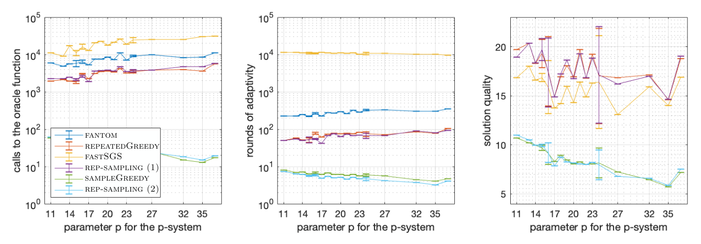
Video Summarization. This problem asks to find a set of representative frames for a given video. We use Determinantal Point Processes to select a diverse set of frame. In order to get better summaries, we employ a face-recognition tool to identify faces in each segment. This experiment is described in Section 8, and the results are displayed in Figure 1.
- •
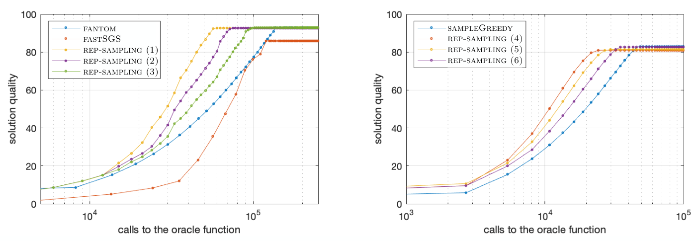
Bayesian D-Optimality. Here, the goal is to design an experiment that maximizes the expected utility of the outcome, using preliminary observations. We use observations from the Berkeley Earth data-set to select thermal stations around the world, to measure the temperature with. This experiment is described in Section 9, and the results are displayed in Figure 2.
The code and the datasets are available upon request.
8 Video Summarization
We study an application of our setting to a data summarization task: Given a video consisting of ordered frames, choose a subset of frames that gives a descriptive overview of the video. An effective way to select a diverse set of items is to apply Determinantal Point Processes (Macchi 1975). For a thorough survey on Determinantal Point Processes and their applications, we refer the reader to Kulesza and Taskar 2012.
For a set of items , a Determinantal Point Process (DPP) defines a discrete probability distribution over all subsets as , where is a positive semidefinite matrix, is the determinant of the sub-matrix of indexed by and is the -identity matrix. Intuitively, if expresses pairwise similarity, then the DPP prefers diversity.
In our setting, each item corresponds to a frame of a video segment. For each frame , we compute a feature vector , consist of both visual features, such as color and SIFT features (Kulesza and Taskar 2011), and qualitative information, such as size, colorfulness and luminosity. Following Gong et al. 2014, we parameterize as , where . We then learn the parameters and using a neural network.
We select a representative summary by maximizing the function . We impose the following additional side constraints. First, we impose an upper-bound on the maximum number of frames of each summary. Then, we partition each video into segments, and define a partition matroid to select at most frames in each segment . Following Mirzasoleiman et al. 2018; Feldman et al. 2018, we also use a face-recognition tool to identify actors in each movie, and select a summary containing at most frames showing face . This additional constraint corresponds to a -system , with all frames containing face .11 1 The parameter is estimated by counting the total number of distinct faces that appear in more than frames. In our experiments, the parameters are always set to a fixed constant for all videos. Hence, the only variable that affects is the total number of distinct faces in each movie.
For our experimental investigation, we use movies from the Frames Labeled In Cinema (FLIC) data-set (Sapp and Taskar 2013). We consider all movies in this data-set with at least frames, as to highlight performance when dealing with large problem size.
The results are displayed in Figure 1, where we describe the parameter choice for each algorithm. For each non-deterministic algorithm, results are the sample mean of independent runs. We observe that, for different parameter choice, our algorithm outperforms fantom and the FastSGS, and it has better adaptivity than the greedy algorithms. The solution quality for the sampleGreedy and rep-sampling, with parameters as in Lemma 3, is worse on these instances.
9 Bayesian D-Optimality
Bayesian experimental design provides a general framework to select a set of experiments, that maximize the expected utility of the outcome. Formally, we want to estimate the parameter of a function , where is an error. In this framework, the input is generated by a set of experiments. Assuming that parameters are equipped with a prior, Bayesian optimality criteria are useful in identifying the right experiments to perform, in order to generate the input .
We focus on linear regressions of the form , with , and . Furthermore, we assume independent and homoscedastic noise. We approach experimental design with the D-optimality criterion, although other methods can be used to this end (Krause et al. 2008). This criterion consists of maximizing the determinant of the Fisher information matrix. As shown in Sebastiani and Wynn 2000, for regressions as described above the D-optimality criterion is equivalent to maximizing the entropy.
We apply the Bayesian D-optimality criterion to the following setting. Consider a data-set consisting of monthly temperatures measured by thermal stations at different locations, over a period of time. We want to collect data to perform a regression for a model explaining the temperature variation from one measurements to the other one. Here, collecting temperatures with a single station corresponds to performing an experiment, and the goal is to identify appropriate stations to perform future measurements with.
Assuming independent and homoscedastic noise, we search for a feasible set of stations maximizing the entropy. Since temperature variation series follow a Gaussian process (Krause et al. 2008; Friedrich et al. 2019), the entropy is defined as , with a subset of stations, and the covariance matrix. The function is the determinant of the covariance matrix corresponding to a set of stations. Note that the function is submodular and non-monotone. We consider an upper-bound on the solution size as a side constraint. Furthermore, we group stations that are located in the same geographical area, and we impose an upper-bound on the number of stations that can be chosen in each group. This additional constraint is useful when stations are not distributed uniformly across a territory (see Friedrich et al. 2019). In our experiment, geographical areas correspond to continents. We remark that, if only a single cardinality constraint is given, then Bayesian optimality criteria can be optimized well via regularized Determinantal Point Processes (Derezinski et al. 2020).
For our experiments we consider the Berkeley Earth climate data-set (http://berkeleyearth.org/data/). This data-set combines billion temperature reports from preexisting data archives, for over unique stations worldwide. We run all algorithms with parameters described as in Figure 2 for a fixed time budget.
In Figure 2, we report on the average solution quality achieved by each algorithm, after a fixed number of oracle calls. We observe that the rep-sampling gets to a good solution more quickly that the other algorithms. All algorithms find similar solution qualities, for unlimited time budget, with the fantom and rep-sampling. slightly outperforming the other algorithms.
10 Conclusion
In this paper, we develop the first algorithm for non-monotone submodular maximization under -system and -extendible system side constraints, with poly-logarithm adaptivity (see Lemma 2 and Theorem 3). This algorithm also competes with previous known results in terms of the query complexity and approximation guarantee (see Table 1).
We consider two applications and study the performance of our algorithm against several other algorithms suitable for this problem. We observe that our algorithms has superior adaptivity, and that it competes in terms of the query complexity (see Figure 1-2).
11 Acknowledgements
We would like to thank Christopher Weyand for helping the authors to develop some of the code used for the experiments. We would like to thank Martin Schirneck for useful discussion on previous related work. This research has been partly funded by the Federal Ministry of Education and Research of Germany in the framework of KI-LAB-ITSE (project number 01IS19066).
References
- Badanidiyuru and Vondrák [2014] Ashwinkumar Badanidiyuru and Jan Vondrák. Fast algorithms for maximizing submodular functions. In Proc. of SODA, pages 1497–1514, 2014.
- Badanidiyuru et al. [2014] Ashwinkumar Badanidiyuru, Baharan Mirzasoleiman, Amin Karbasi, and Andreas Krause. Streaming submodular maximization: massive data summarization on the fly. In Proc. of KDD, pages 671–680, 2014.
- Balcan and Harvey [2011] Maria-Florina Balcan and Nicholas J. A. Harvey. Learning submodular functions. In proc. of STOC, pages 793–802, 2011.
- Balkanski and Singer [2018a] Eric Balkanski and Yaron Singer. Approximation guarantees for adaptive sampling. In Proc. of ICML, pages 393–402, 2018a.
- Balkanski and Singer [2018b] Eric Balkanski and Yaron Singer. The adaptive complexity of maximizing a submodular function. In Proc. of STOC, pages 1138–1151, 2018b.
- Balkanski et al. [2017] Eric Balkanski, Aviad Rubinstein, and Yaron Singer. The limitations of optimization from samples. In Proc. of STOC, pages 1016–1027, 2017.
- Balkanski et al. [2018] Eric Balkanski, Adam Breuer, and Yaron Singer. Non-monotone submodular maximization in exponentially fewer iterations. In Proc. of NeurIPS, pages 2359–2370, 2018.
- Balkanski et al. [2019] Eric Balkanski, Aviad Rubinstein, and Yaron Singer. An optimal approximation for submodular maximization under a matroid constraint in the adaptive complexity model. In Proc. of STOC, pages 66–77, 2019.
- Buchbinder et al. [2014] Niv Buchbinder, Moran Feldman, Joseph Naor, and Roy Schwartz. Submodular maximization with cardinality constraints. In Proc. of SODA, pages 1433–1452, 2014.
- Buchbinder et al. [2015] Niv Buchbinder, Moran Feldman, Joseph Naor, and Roy Schwartz. A tight linear time (1/2)-approximation for unconstrained submodular maximization. SIAM Journal of Computing, 44(5):1384–1402, 2015.
- Chakrabarti and Kale [2015] Amit Chakrabarti and Sagar Kale. Submodular maximization meets streaming: matchings, matroids, and more. Mathematical Programming, 154(1-2):225–247, 2015.
- Chaloner and Verdinelli [1995] Kathryn Chaloner and Isabella Verdinelli. Bayesian experimental design: A review. Statistical Science, 10:273–304, 1995.
- Chekuri and Pál [2005] Chandra Chekuri and Martin Pál. A recursive greedy algorithm for walks in directed graphs. In Proc. of FOCS, pages 245–253, 2005.
- Chekuri and Quanrud [2019] Chandra Chekuri and Kent Quanrud. Parallelizing greedy for submodular set function maximization in matroids and beyond. In Moses Charikar and Edith Cohen, editors, Proc. of STOC, pages 78–89, 2019.
- Chekuri et al. [2014] Chandra Chekuri, Jan Vondrák, and Rico Zenklusen. Submodular function maximization via the multilinear relaxation and contention resolution schemes. SIAM Journal of Computing, 43(6):1831–1879, 2014.
- Chekuri et al. [2015] Chandra Chekuri, Shalmoli Gupta, and Kent Quanrud. Streaming algorithms for submodular function maximization. In Proc. of ICALP, pages 318–330, 2015.
- Chen et al. [2019] Lin Chen, Moran Feldman, and Amin Karbasi. Unconstrained submodular maximization with constant adaptive complexity. In Proc. of STOC, pages 102–113, 2019.
- Das and Kempe [2018] Abhimanyu Das and David Kempe. Approximate submodularity and its applications: Subset selection, sparse approximation and dictionary selection. Journal of Machine Learning Research, 19:3:1–3:34, 2018.
- Derezinski et al. [2020] Michal Derezinski, Feynman Liang, and Michael W. Mahoney. Bayesian experimental design using regularized determinantal point processes. In Proc. of AISTATS, volume 108, pages 3197–3207, 2020.
- Ene and Nguyen [2019] Alina Ene and Huy L. Nguyen. Submodular maximization with nearly-optimal approximation and adaptivity in nearly-linear time. In Proc. of SODA, pages 274–282, 2019.
- Ene et al. [2019] Alina Ene, Huy L. Nguyen, and Adrian Vladu. Submodular maximization with matroid and packing constraints in parallel. In Proceedings of STOC, pages 90–101, 2019.
- Fahrbach et al. [2019a] Matthew Fahrbach, Vahab S. Mirrokni, and Morteza Zadimoghaddam. Non-monotone submodular maximization with nearly optimal adaptivity and query complexity. In Proc. of ICML, pages 1833–1842, 2019a.
- Fahrbach et al. [2019b] Matthew Fahrbach, Vahab S. Mirrokni, and Morteza Zadimoghaddam. Submodular maximization with nearly optimal approximation, adaptivity and query complexity. In Proc. of SODA, pages 255–273, 2019b.
- Feige [1998] Uriel Feige. A threshold of ln n for approximating set cover. Journal of the ACM, 45(4):634–652, 1998.
- Feige et al. [2011] Uriel Feige, Vahab S. Mirrokni, and Jan Vondrák. Maximizing non-monotone submodular functions. SIAM Journal of Computing, 40(4):1133–1153, 2011.
- Feldman et al. [2011] Moran Feldman, Joseph Naor, and Roy Schwartz. Nonmonotone submodular maximization via a structural continuous greedy algorithm - (extended abstract). In Proc. of ICALP, pages 342–353, 2011.
- Feldman et al. [2017] Moran Feldman, Christopher Harshaw, and Amin Karbasi. Greed is good: Near-optimal submodular maximization via greedy optimization. In Proc. of COLT, pages 758–784, 2017.
- Feldman et al. [2018] Moran Feldman, Amin Karbasi, and Ehsan Kazemi. Do less, get more: Streaming submodular maximization with subsampling. In Proc. of NeurIPS, pages 730–740, 2018.
- Feldman et al. [2020] Moran Feldman, Christopher Harshaw, and Amin Karbasi. Simultaneous greedys: A swiss army knife for constrained submodular maximization. CoRR, abs/2009.13998, 2020.
- Fisher et al. [1978] M. Fisher, George Nemhauser, and Laurence Wolsey. An analysis of approximations for maximizing submodular set functions - II. Mathematical Programming, 14:73–87, 03 1978.
- Friedrich et al. [2019] Tobias Friedrich, Andreas Göbel, Frank Neumann, Francesco Quinzan, and Ralf Rothenberger. Greedy maximization of functions with bounded curvature under partition matroid constraints. In Proc. of AAAI, pages 2272–2279, 2019.
- Gong et al. [2014] Boqing Gong, Wei-Lun Chao, Kristen Grauman, and Fei Sha. Diverse sequential subset selection for supervised video summarization. In Proc. of NIPS, pages 2069–2077, 2014.
- Gupta et al. [2010] Anupam Gupta, Aaron Roth, Grant Schoenebeck, and Kunal Talwar. Constrained non-monotone submodular maximization: Offline and secretary algorithms. In Proc. of WINE, pages 246–257, 2010.
- Karp et al. [1988] Richard M. Karp, Eli Upfal, and Avi Wigderson. The complexity of parallel search. Journal of Computer System Science, 36(2):225–253, 1988.
- Krause et al. [2008] Andreas Krause, Ajit Paul Singh, and Carlos Guestrin. Near-optimal sensor placements in gaussian processes: Theory, efficient algorithms and empirical studies. Journal of Machine Learning Research, 9:235–284, 2008.
- Kulesza and Taskar [2011] Alex Kulesza and Ben Taskar. k-dpps: Fixed-size determinantal point processes. In Proc. of ICML, pages 1193–1200, 2011.
- Kulesza and Taskar [2012] Alex Kulesza and Ben Taskar. Determinantal point processes for machine learning. Foundations and Trends in Machine Learning, 5(2-3):123–286, 2012.
- Kumar et al. [2015] Ravi Kumar, Benjamin Moseley, Sergei Vassilvitskii, and Andrea Vattani. Fast greedy algorithms in mapreduce and streaming. ACM Transaction on Parallel Computing, 2(3):14:1–14:22, 2015.
- Lee et al. [2009] Jon Lee, Vahab S. Mirrokni, Viswanath Nagarajan, and Maxim Sviridenko. Non-monotone submodular maximization under matroid and knapsack constraints. In Proc. of STOC, pages 323–332, 2009.
- Li et al. [2020] Wenzheng Li, Paul Liu, and Jan Vondrák. A polynomial lower bound on adaptive complexity of submodular maximization. CoRR, abs/2002.09130, 2020.
- Lin and Bilmes [2010] Hui Lin and Jeff Bilmes. Multi-document summarization via budgeted maximization of submodular functions. In Proc. of NAACL-HLT, pages 912–920, 2010.
- Macchi [1975] Odile Macchi. The coincidence approach to stochastic point processes. Advances in Applied Probability, 7(1):83–122, 1975. doi: 10.2307/1425855.
- Mestre [2006] Julián Mestre. Greedy in approximation algorithms. In Proc. of ESA, pages 528–539, 2006.
- Mirzasoleiman et al. [2013] Baharan Mirzasoleiman, Amin Karbasi, Rik Sarkar, and Andreas Krause. Distributed submodular maximization: Identifying representative elements in massive data. In Proc. of NIPS, pages 2049–2057, 2013.
- Mirzasoleiman et al. [2015] Baharan Mirzasoleiman, Ashwinkumar Badanidiyuru, Amin Karbasi, Jan Vondrák, and Andreas Krause. Lazier than lazy greedy. In Proc. of AAAI, pages 1812–1818, 2015.
- Mirzasoleiman et al. [2016] Baharan Mirzasoleiman, Ashwinkumar Badanidiyuru, and Amin Karbasi. Fast constrained submodular maximization: Personalized data summarization. In Proc. of ICML, pages 1358–1367, 2016.
- Mirzasoleiman et al. [2018] Baharan Mirzasoleiman, Stefanie Jegelka, and Andreas Krause. Streaming non-monotone submodular maximization: Personalized video summarization on the fly. In Sheila A. McIlraith and Kilian Q. Weinberger, editors, Proc. of AAAI, pages 1379–1386, 2018.
- Nemhauser et al. [1978] George L. Nemhauser, Laurence A. Wolsey, and Marshall L. Fisher. An analysis of approximations for maximizing submodular set functions - I. Mathematical Programming, 14(1):265–294, 1978.
- Rosenfeld et al. [2018] Nir Rosenfeld, Eric Balkanski, Amir Globerson, and Yaron Singer. Learning to optimize combinatorial functions. In Proc. of ICML, pages 4371–4380, 2018.
- Sapp and Taskar [2013] Benjamin Sapp and Ben Taskar. Modec: Multimodal decomposable models for human pose estimation. In Proc. of CVPR, 2013.
- Sebastiani and Wynn [2000] P. Sebastiani and H.P. Wynn. Maximum entropy sampling and optimal bayesian experimental design. Journal of the Royal Statistical Society: Series B (Statistical Methodology), 62(1):145–157, 2000.
- Sviridenko [2004] Maxim Sviridenko. A note on maximizing a submodular set function subject to a knapsack constraint. Operation Research Letters, 32(1):41–43, 2004.
- Thompson [1990] Steven K. Thompson. Adaptive cluster sampling. Journal of the American Statistical Association, 85(412):1050–1059, 1990.
- Valiant [1984] Leslie G. Valiant. A theory of the learnable. Communication of the ACM, 27(11):1134–1142, 1984.
Appendix
Appendix A Notation
Here, we discuss the notation that will be used throughout the proofs in the Appendix, which is also discussed in the main body of the paper.
For any submodular function and sets , we define the marginal value of with respect to as . Note that, if only attains non-negative values, it holds that for all .
We always use the notation introduced in Problem 1, and we always denote with opt a solution to Problem 1. Furthermore, we always denote with the size of the ground set , i.e., is the number of singletons in our solution space. We denote with the maximum size of any feasible solution in . This quantity is sometimes called the rank.
We denote with the parameters as in Algorithm 3. Sets and are as in Algorithm 3, and we denote with the ground set for the rand-sampling algorithm, during the -th iteration of the for-loop lines 2-6 of Algorithm 3.
Furthermore , and are as in Algorithm 2 and Algorithm 3. We denote with the problem size, and we denote with the maximum size of a feasible solution in .
Appendix B Proof of Lemma 5
In this section, we prove a lemma that is useful to prove the desired approximation guarantee. Throughout the section, we always implicitly assume that parameters for Algorithm 2 and Algorithm 3 are as in Theorem 1, i.e., and . The following lemma holds.
Lemma 5.
It holds , for all sets .
On a high level, we prove that is an upper-bound for the best possible improvement up to a multiplicative constant, and that the marginal contribution of any point added to the current solution does not exceed in expected value, up to a multiplicative constant. We then combine this fact with the defining properties of the -system to prove the claim, which holds for non-monotone functions. With this lemma, we prove that Algorithm 3 yields, in expectation, a constant-factor approximation guarantee for Problem 1.
B.1 Preliminary Results
In order to prove Lemma 5, we need the following technical proposition.
Proposition 1 (Proposition 2.2 in Fisher et al. 1978).
Let be two sequences of non-negative real numbers. Suppose that it holds
for all and for all . Then
B.2 Additional Lemmas
We first prove the following result, which follows from Lemma 2 in Balkanski et al. 2019.
Lemma 6.
Fix an index , and let be as in Algorithm 2, as it runs over the set . Then it holds
Proof.
We prove the claim by induction on the iterations of Algorithm 2. The base case trivially holds, due to the definition of . Suppose that at some point the current solution is updated to . We have that
where the first inequality uses the submodularity property of ; the second inequality holds since ; the last inequality follows due to the inductive hypothesis.
We now show that the claim holds when is updated to . At this point, it holds , and each point such that was discarded during a previous iteration. Denote with the solution at the iteration when was discarded, and let be the next set of points added to . Since was discarded, then one of the following two conditions must hold:
- 1.
;
- 2.
.
In the first case, due to the downward-closed property of it holds , which contradicts the definition of . In the latter case it holds
where the first inequality uses the fact that is submodular. The claim follows. ∎
We also need an additional lemma, to prove that Algorithm 3 gives a constant-factor approximation for Problem 1.
Lemma 7.
Fix an index , and let be as in Algorithm 2, as it optimizes the function over the set . Denote with the points of , sorted as they were added to it. It holds
Proof.
First, suppose that the constant is updated after the point is added to the current solution. In that case, by definition of the set , every point such that yields . Hence, the claim holds.
Suppose now that the constant is not updated after the point is added to the current solution. Define the set . We first claim that the point is chosen uniformly at random over the set . In fact, if is added to the current solution, then there exists a set as in Line 5 of Algorithm 1 such that . Let be an index such that . Due to the downward-closed property of it holds . Hence, is chosen uniformly at random among all points such that .
Then
where we have used that and that the point is chosen uniformly at random over the set .
We now prove that . To this end, we first note that , for all indices . Fix a point . Then, this point yields and . By the downward-closed property of we get , and by submodularity we get . Hence, and as claimed. It follows that the binary-search sub-routine of Algorithm 2 terminates whenever , which implies that . The claim follows since it holds . ∎
B.3 Proof of Lemma 5
Using Proposition 1, Lemma 6-7, we can prove Lemma 5. This proof uses ideas in Gupta et al. 2010.
Proof of Lemma 5.
Denote with the points of in the order that they were added to . Define the set
Note that this set consists of all points of such that their marginal contribution is above , when added to the current solution. First, fix a set , and suppose that for all indices . Define the sets . Since the system is downward-closed, then . Define the sets . Note that these sets consist of all points in that yield a feasible solution when added to , but that violate side constraints when added to .
We now claim that the set is a maximal independent set for
To this end, note that the set is independent by definition, and that any point is such that . Hence is maximal as claimed. Note also that is an independent set, due to the subset-closure of . Since is a -system, then it holds
| (1) |
Furthermore, using submodularity and Lemma 6 it holds
where the last inequality follows from submodularity. Combining this with (1) and Proposition 1, we get
where the last inequality uses submodularity. Hence, rearranging yields . If we unfix the set and take the expected value, and using Lemma 7 we get
| (2) |
Using Lemma 7 again, we have that , for all points added to . It follows that , with the first point added to . Then, from the definition of it follows that . Hence, using submodularity and the linearity of the expected value, we get
| (3) |
where we have used submodularity.
Appendix C Proof of Theorem 5
C.1 Preliminary results.
In our analysis we consider the following well-known result.
Lemma 8 (Theorem 2.1 in Feige et al. 2011).
Let be a set chosen uniformly at random. Then it holds , with the subset attaining the maximum -value.
Furthermore, we also consider the following properties of submodular functions.
Lemma 9 (Lemma 10 in Feldman et al. 2017).
For any fixed -tuple of mutually disjoint sets it holds .
Lemma 10 (Lemma 11 in Feldman et al. 2017).
Let be a non-negative submodular function. For every three sets it holds .
C.2 Proof of Theorem 1
Proof of Theorem 1.
Fix an -tuple of sets for Algorithm 3, and consider the sets , for all . Note that it holds . Hence, , where the last inequality uses submodularity.
Unfixing the sets and taking the expected value yields
| (4) |
for all indices . We have that it holds
where the first inequality follows from Lemma 9; the second inequality follows from Lemma 10; the third inequality follows from (4) and Lemma 5; the fourth inequality follows from Lemma 8; the last inequality follows since is maximum over and . The claim follows by rearranging the inequality above. ∎
Appendix D Proof of Lemma 1
Proof.
First, note that Algorithm 1 requires no function evaluation, and it always return a sequence of length at most .
At each step of Algorithm 2, the binary-search sub-routine requires iterations, sine the set has size at most . Each iteration of this sub-routine requires rounds of adaptivity, and function evaluations.
Note also that the while-loop, lines 5-10 of Algorithm 2 terminates after at most iterations. In fact, we have that , and that at each iteration the size of the new set decreases of a multiplicative factor of . Similarly, the outer while-loop, lines 4-13 of Algorithm 2 terminates after at most iterations.
Hence, each call of Algorithm 2 requires rounds of adaptivity. Similarly, since the binary-search sub-routine requires function evaluations, then the query complexity is . ∎
Appendix E Proof of Lemma 2
We perform the run time analysis for an optimal choice of the parameter . We have that the following theorem holds. See 2
Proof.
We start with the approximation guarantee. Denote with an approximate solution found by Algorithm 3, and let opt be the optimal solution for Problem 1. Then, from Theorem 1 we get
Substituting and rearranging yields
Hence, the claim on the approximation guarantee follows. The upper-bounds on the adaptivity, depth, and total number of calls to the valuation oracle function follow directly from Lemma 1. ∎
Appendix F Proof of Lemma 4
In this section, we perform the run time analysis for Algorithm 3 with respect to the calls to the independence oracle for the -system. The following lemma holds. See 4 In order to prove this Lemma, we use the following well-known result.
Theorem 2 (Theorem 6 in Karp et al. 1988).
Algorithm 1 terminates after steps.
Proof.
We first observed that the independence oracle for the -system is called by Algorithm 1, and also by Algorithm 2.
Since at each iteration of Algorithm 1, queries to the oracle for the -system are independent, the from Theorem 2 it follows that Algorithm 1 requires rounds of independent calls to the oracle for the -system. Furthermore, all calls to the independence oracle for the -system in Algorithm 2 are independent. Combining these observations with Lemma 1 it follows that Algorithm 3 requires rounds of independent calls to the oracle for the -system.
The claim follows, since at each round at most calls to the oracle for the -system are executed in parallel. ∎
Appendix G Proof of Theorem 3
G.1 Preliminary Results.
In order to prove Theorem 3 we use the following well-known result.
Lemma 11 (Lemma 2.2 in Buchbinder et al. 2014).
Let be a set such that each element appears in with probability at most . Then it holds .
G.2 Additional Lemmas.
In this section, we prove the following theorem. See 3 In order to prove this theorem, we introduce additional notation. First of all, since , we need not specify the index on the input search space and solution of Algorithm 2, and we simply use the notation and . Again we define . Furthermore, we define an ordering of the points , with the -th point sampled by Algorithm 2 during run time. All points of that are not sampled during run time, are placed at the end of the sequence in random order. Furthermore, we define the sets , and we define the sequence as
For each point , denote with an indicator function such that if is sampled as part of a random feasible sequence , and otherwise. We also consider a sequence of sets defined recursively as
- •
;
- •
if , then is a set of minimum size such that ;
- •
if , , and , then ;
- •
if and , or if , then .
Finally, we define the set .
Following this notation, we first prove the following lemma.
Lemma 12.
Fix all random decisions of Algorithm 2. Then it holds
Proof.
First, we prove that it holds
| (5) |
To this end, note that since , then it holds for all . Hence, by the termination criterion of Algorithm 2, we have that .
where we have used submodularity. Then (5) follows.
Next, we prove that it holds
| (6) |
Note that the claim of this lemma follows by combining (5) and (6).
To prove (6), we first observe that the sets are mutually disjoint, and we can write . Using this equality, we have that
where the first equation is the telescopic sum, the second one uses submodularity, together with the fact that , and the third one use submodularity again. Then (6) follows from the definition of . ∎
Next, using Lemma 12 we prove the following result.
Lemma 13.
It holds
Proof.
We first observe that if , then the claim holds since . Hence, we prove the claim by conditioning on the event . In this case, the point is added to w.p. .
If is not added to the current solution, then , and conditioning on the event we get
where we have used that . Furthermore, if the solution is added to , then the set has size at most , since is a -extendible system. Hence,
The claim follows combining the two chains of inequalities above, together with Lemma 6 and Lemma 7. ∎
We also need the following lemma, to prove the main theorem.
Lemma 14.
It holds
Proof.
For each , let be a random variable whose value is equal to in the increase in the value of the current solution when added to it. Note that if yields , then because it cannot be added to the current solution. Then,
| (7) |
The claim follows using Lemma 13, and using the law of total probability and linearity of the expected value. ∎
G.3 Proof of Theorem 3.
We now have all necessary tools to prove the main theorem.
Proof of Theorem 3.
Combining Lemma 12, taking the expected value, and combining with Lemma 14 we get
| (8) |
Denote with the points of in the order that they were added to . From Lemma 7 and submodularity, we have that , for all points added to . It follows that , with the first point added to . Hence, from the definition of , and since due to feasibility, we get . Substituting in (8) we get
To conclude the proof, we observe that the function is a submodular function. Since each element of appears in w.p. at most , then by Lemma 11 we get
The claim follows. ∎