Interview Hoarding We thank Anna Sorensen and Alkas Baybas for raising the question that sparked this paper. We also thank Alex Chan, Adrienne Quirouet, Assaf Romm, Al Roth, Erling Skancke, Colin Sullivan, William Thomson, and seminar audiences at North Carolina State University, Stanford, University of Arizona, and University of Lausanne for helpful comments and discussions. We are grateful for the feedback from Federico Echenique and two anonymous referees that helped us improve the paper substantially.

Vikram Manjunath University of Ottawa vikramma@gmail.com Thayer Morrill North Carolina State University thayer_morrill@ncsu.edu

Abstract

Many centralized matching markets are preceded by interviews between participants. We study the impact on the final match of an increase in the number of interviews for one side of the market. Our motivation is the match between residents and hospitals where, due to the COVID-19 pandemic, interviews for the 2020-21 season of the National Residency Matching Program were switched to a virtual format. This drastically reduced the cost to applicants of accepting interview invitations. However, the reduction in cost was not symmetric since applicants, not programs, previously bore most of the costs of in-person interviews. We show that if doctors can accept more interviews, but the hospitals do not increase the number of interviews they offer, then no previously matched doctor is better off and many are potentially harmed. This adverse consequence is the result of what we call interview hoarding. We prove this analytically and characterize optimal mitigation strategies for special cases. We use simulations to extend these insights to more general settings.

Keywords: NRMP, Deferred acceptance, Interviews, Hoarding

1 Introduction

Perhaps the most well-known application of matching theory is the entry-level labor market for physicians. In 2021, 37,470 positions were matched through the National Resident Matching Program (NRMP). The matching process consists of two steps. First, each physician interviews with a set of residency programs. Second, programs and physicians submit rank-order lists of those they interview to a centralized clearinghouse. This clearinghouse, run by the NRMP, matches physicians to residency programs using a version of Gale and Shapley 1962’s (Gale and Shapley 1962) Deferred Acceptance (DA) Algorithm (Roth and Peranson 1999).

Both programs and applicants are constrained in the number of interviews they can take part in. Prior to the COVID-19 pandemic, interviews were done in person. These interviews were particularly costly for physicians since they not only had to bear travel expenses but also had to take days off from clinical rotations. The cost to programs was mainly in terms of time. For the 2020-21 matching season, interviews were conducted virtually. While this dramatically decreased the cost of interviews for physicians, it did not substantially change the costs for the programs. We are interested in the implications of this asymmetric change on the eventual match.

Intuitively, it seems possible that a doctor might receive a better match if she accepts more interviews. We show a surprising result. As long as she would have been matched with a program, increasing her interview capacity does not help. Further, we show that even if she would have been unmatched, she can only benefit if she also would have been part of a pair (with some program) that blocked the original matching.¹¹ 1 While the NRMP match is stable with respect to submitted preferences over those one interviews, it may not be stable with respect to actual preferences over all possible matching partners. The match rate for US medical school graduates is typically around 94%.²² 2 Specifically, the match rates in 2017 through 2020 were $94.3\%$ , $94.3\%$ , $93.9\%$ , and $93.7\%$ . These figures are from the NRMP’s “Results and Data: 2021 Main Residency Match”. Our result says that at least this proportion of the doctors does not benefit, but could be harmed, from increasing the number of interviews they participate in.

Increasing the number of interviews a doctor accepts has a negative externality: these interviews can no longer be allocated to other doctors. To illustrate, consider a highly sought after physician: one who is offered interviews at the leading programs and ends up matched with her favorite program. When interviews become cheaper, she accepts more interviews.³³ 3 While we assume that agents have complete information, if there were an arbitrarily small amount of uncertainty about others’ preferences, she would accept additional costless interviews. However, as she would already have matched with her favorite program, the interviews she accepts are from inferior programs. These interviews do not help her: she ultimately matches with the same program as before. Her additional interviews are, in effect, wasted. We refer to this as interview hoarding. Interview hoarding has a cascading affect. The physicians who otherwise would have filled these wasted interview slots now interview with programs they consider inferior. Such a physician may have more interviews, but she does not have better interviews in a precise sense: she rates every new interview as worse than the program she matched with before.

This implies a striking result. If there is an increase to doctors’ interview capacities, but programs do not react, this increase causes the ultimate match to be (Pareto) worse from the matched physicians’ perspective.⁴⁴ 4 The example in Section 1.2 demonstrates that there need not exist a Pareto ranking from the programs’ perspective. These doctors fall into three categories: those who hoard interviews worse than their eventual match; those who receive more but worse interviews; and those who receive fewer and worse interviews. The first category is indifferent between the new outcome and the old. The latter two categories are harmed. Even among unmatched physicians, only those who fall through the cracks—meaning that they are unmatched but would be welcomed by some programs—could potentially benefit from an increase. At a match rate of 94%, this means fewer than 6% of doctors could possibly gain while the overwhelming majority could be harmed.

We are not suggesting that there is no benefit to increasing interviews. We are making two unrealistic assumptions. First, that doctors and programs know their preferences perfectly. Second, that agents, faced with a constraint on the number of interviews they accept, are not strategic.⁵⁵ 5 We follow the approach of Echenique et al. 2020 in assuming complete information about preferences and non-strategic offers and acceptance of interviews. In reality, of course, neither doctors nor programs perfectly know their preferences. The point of interviews is to learn more about a candidate or program. Similarly, both doctors and programs will be strategic in the interviews they accept. We expect a doctor to accept an interview with a ‘‘safety’’ program, one she is sure to match with, while lower ranked programs likely do not invite the very best candidates for interviews so that they do not ‘‘waste’’ their slots. Rather, our results show that these are the only two channels through which doctors may gain from increasing the number of interviews they accept. By doing so, a doctor learns about more programs and has more flexibility to strategize.⁶⁶ 6 If a doctor was previously unmatched but formed a blocking pair with a hospital, then she must have declined that hospital’s interview. Ex-post, this was a strategic mistake. We interpret the doctor’s benefit from increasing her interviews and being matched as a strategic benefit. The advantage of our modeling choices is that they allow us to identify a subtle bottleneck created by interviews that would likely be lost in the analysis of a more complex model.

Having shown that increases to doctors’ interview capacities has adverse welfare consequences, we turn to mitigation policies. We consider policies that limit the numbers of interviews that programs can offer and candidates can accept. Though there are essentially no such policies that always (for every preference profile) yield a stable final matching (Proposition 1), we characterize such policies for “common preferences” (Proposition 2). These are salient preference profiles where every doctor ranks the programs the same way and every program ranks the doctors the same way. The policies we characterize are such that there is a common cap on the number of interviews any program can offer or any candidate can accept. We also show that if the programs’ interview capacities are fixed, say at $l$ , then the number of blocking pairs increases and the match rate decreases as the doctors’ interview cap moves further away from $l$ in either direction (Proposition 3).

Our analytical results can advise policies for more general settings where preferences are not quite common, but have a common component. We use simulations to show that the lessons from our analytical results hold up under weaker assumptions. The optimal policy is for doctors and programs to have the same interview capacity.⁷⁷ 7 This is true whether we define the optimality of a policy as maximizing the expected proportion of positions that are filled or minimizing the expected number of blocking pairs. In fact, these objectives are equivalent.

1.1 Related Literature

While there is a large literature on the post-interview NRMP match,⁸⁸ 8 See the multitude of papers following Roth and Peranson 1999. there are relatively few papers that incorporate the pre-match interview process. One of the first to explicitly model interviews in the classic one-to-one matching model is Lee and Schwarz 2017. In their model, before participating in a centralized, two-sided match, firms learn their preferences over workers by engaging in costly interviews. They show that even if firms and workers interview with exactly the same numbers of agents, the extent of unemployment in the final match depends critically on the overlap between the sets of workers that firms interview. Three other recent papers that incorporate pre-match interviews include Kadam 2021, Beyhaghi 2019, and Echenique et al. 2020.

Like our paper, Kadam 2021 considers the implications of loosened interview constraints for doctors. However, the focus is on the strategic allocation of scarce interview slots. For the sake of tractability, the analysis is for a stylized model of large markets. Under the assumption of common preferences over programs, they show that increasing doctors’ capacities may increase total surplus, but not in a Pareto-improving way. Moreover, the match rate decreases. He also highlights that when preferences are not necessarily common, the effect is ambiguous, since increased interview capacities dilute doctors’ signaling ability.

Beyhaghi 2019 also performs a strategic analysis of a stylized large market model. However, they consider a slightly different set up with application caps for doctors and interview caps for programs. While similar, application caps are not the same as interview caps: they constrain the number of programs a doctor can express interest in at the outset of the interview matching phase, but not the number of interviews she can accept at the end. In their model, inequity in the application caps decreases the expected total surplus. Moreover, when interview capacity is low, low application caps are socially desirable.

In our model, agents do not choose interviews strategically. Determining the optimal set of interviews is closely related to the portfolio choice problems of Chade and Smith 2006 and Ali and Shorrer 2021. Both of these solve for the optimal portfolio when an agent chooses a portfolio of costly, stochastic options, but only consumes one of the realizations. In order to apply the optimal solution to the interview scheduling problem, one would have to pin down precisely the probability of any given pair matching. This is what makes strategic analysis of the problem intractable without severe simplifying assumptions (such as those in the papers we have mentioned above).

As in Echenique et al. 2020, which is methodologically closest to ours, we sidestep this issue. They explain a puzzling empirical pattern resulting from the NRMP match: 46.3% of the physicians were matched to their top ranked residency programs and 71.1% where matched to a program they ranked in their top three. These statistics seem to contradict surveys indicating that many doctors have similar preferences over residency programs. They provide an explanation for this phenomenon by pointing out the importance of the interviewing process that precedes the match. Roughly speaking, the pre-match interviewing process restricts the preferences that the physicians actually submit to the NRMP. Therefore, a proper interpretation is not that the physicians matched with their most preferred programs but rather that they matched with their most preferred programs among those they interviewed with.

Our work is complementary with these papers in the sense that they highlight the importance of understanding the prematch interviews for properly evaluating the NRMP match itself.

1.2 Motivating Example

We present the intuition behind the welfare loss from increased interview capacity for doctors with a simple example. Consider a market with five doctors $\left\{d_{1},\ldots,d_{5}\right\}$ and four hospitals $\left\{h_{1},\ldots,h_{4}\right\}$ . Their preferences are as follows:

$d_{1}$	$d_{2}$	$d_{3}$	$d_{4}$	$d_{5}$	$h_{1}$	$h_{2}$	$h_{3}$	$h_{4}$
$h_{1}$	$h_{1}$	$h_{1}$	$h_{3}$	$h_{4}$	$d_{1}$	$d_{1}$	$d_{1}$	$d_{1}$
$h_{4}$	$h_{2}$	$h_{2}$	$h_{4}$	$h_{3}$	$d_{2}$	$d_{2}$	$d_{4}$	$d_{5}$
$h_{3}$	$h_{4}$	$h_{3}$	$h_{2}$	$h_{1}$	$d_{3}$	$d_{4}$	$d_{5}$	$d_{3}$
$h_{2}$	$h_{3}$	$h_{4}$	$h_{1}$	$h_{2}$	$d_{5}$	$d_{3}$	$d_{2}$	$d_{2}$
					$d_{4}$	$d_{5}$	$d_{3}$	$d_{4}$

Suppose that the interview capacities of the doctors and hospitals are:

$d_{1}$	$d_{2}$	$d_{3}$	$d_{4}$	$d_{5}$	$h_{1}$	$h_{2}$	$h_{3}$
$2$	$1$	$1$	$1$	$1$	$2$	$1$	$1$

Interviews are initially offered by hospitals: $h_{1}$ invites $d_{1}$ and $d_{2}$ , and $h_{2},h_{3},$ and $h_{4}$ all invite $d_{1}$ . As $d_{1}$ can accept only two invitations, she turns $h_{2}$ and $h_{3}$ down. Hospital $h_{2}$ then offers an interviews to $d_{2}$ and $h_{3}$ invites $d_{4}$ . Since $d_{2}$ can only accept one interview, she declines $h_{2}$ ’s invitation. Then, $h_{2}$ invites and is turned down by $d_{4}$ . Finally, $h_{2}$ invites $d_{3}$ who accepts the invitation. The final interviews are:

$d_{1}$	$d_{2}$	$d_{3}$	$d_{4}$	$d_{5}$
$\{h_{1},h_{4}\}$	$\{h_{1}\}$	$\{h_{2}\}$	$\{h_{3}\}$	$\varnothing$

The final matching is computed by applying the doctor-proposing Deferred Acceptance algorithm to the agent preferences (restricted to agents they interview with). The outcome is therefore:

$d_{1}$	$d_{2}$	$d_{3}$	$d_{4}$	$d_{5}$
$h_{1}$		$h_{2}$	$h_{3}$

Now suppose each doctor can accept one more invitation but the hospitals’ interview capacities remain the same. In this case $d_{1}$ does not reject $h_{3}$ ’s invitation in the first round of interview invitations. Similarly, $d_{2}$ does not reject $h_{2}$ ’s invitation in the second round. The interview schedule is:

$d_{1}$	$d_{2}$	$d_{3}$	$d_{4}$
$\left\{h_{1},h_{3},h_{4}\right\}$	$\{h_{1},h_{2}\}$	$\varnothing$	$\varnothing$	$\varnothing$

This leads to the final matching:

$d_{1}$	$d_{2}$	$d_{3}$	$d_{4}$
$h_{1}$	$h_{2}$

Doctors $d_{3}$ and $d_{4}$ are worse off despite being able to accept more interviews. The only doctor who gains is $d_{2}$ .⁹⁹ 9 The programs, however, are not unanimously better or worse off: $h_{2}$ is better off while $h_{3}$ is worse off. We make a few observations about the winners and losers from the increased interview capacities:

1.

Doctor $d_{2}$ , the only doctor who gained, was among the doctors who were originally unmatched.
2.

The original matching was not stable. Each of $d_{2}$ and $d_{5}$ was part of a blocking pair ( $d_{2}$ blocked with $h_{2}$ and $d_{5}$ blocked with $h_{4}$ ). Specifically, the only doctor to gain was among doctors who blocked.
3.

Despite being part of a pair that blocked the original matching, $d_{5}$ did not regret turning down any interview invitations, while $d_{2}$ did.¹⁰¹⁰ 10 By “regret” we mean that she turned down an interview invitation from a hospital that she preferred to her final matching. In particular, the only doctor who gained did previously reject an invitation that she ended up regretting.

These observations are not specific to this example. We show that (Theorem 1), in general, a doctor can only gain from an increase to interview capacities if she was originally unmatched, she was part of a blocking pair, and she regretted rejecting an interview invitation.

2 The Model

A market consists of a triple $(D,H,P)$ , where $D$ is a finite set of doctors, $H$ is a finite set of hospitals, and $P$ is a profile of strict preferences for the doctors and hospitals. For each $h\in H$ , $\mathcal{P}_{h}$ is the set of strict preferences over $D\cup\{h\}$ , and for each $d\in D$ , $\mathcal{P}_{d}$ is the set of strict preferences over $H\cup\{d\}$ . The set of preference profiles is $\mathcal{P}\equiv\times_{i\in H\cup D}\mathcal{P}_{i}$ .

There are two phases to the matching process. The first is a decentralized interview phase and the second is the centralized matching phase. The former involves many-to-many matching while the latter is a standard one-to-one matching problem (Roth and Sotomayor 1990).

A many-to-many matching is a function $\nu:H\cup D\rightarrow 2^{H\cup D}$ such that, for each $d\in D$ and $h\in H$ , $\nu(d)\subseteq H$ , $\nu(h)\subseteq D$ , and $h\in\nu(d)$ if and only if $d\in\nu(h)$ .

For each $h\in H$ , let ${\iota_{h}}\in\mathbb{N}$ be $h$ ’s interview capacity. Similarly, for each $d\in D$ , let $\kappa_{d}\in\mathbb{N}$ be $d$ ’s interview capacity. We call the profile $(\iota,\kappa)=((\iota_{h})_{h\in H}(\kappa_{d})_{d\in D})$ the interview capacity profile. An interview matching is a many-to-many matching $\nu$ such that for every doctor $d$ , $|\nu(d)|\leq\kappa_{d}$ and for every hospital $h$ , $|\nu(h)|\leq\iota_{h}$ .

An interview matching $\nu$ is pairwise stable if there is no doctor-hospital pair $(d,h)$ such that $h\notin\nu(d)$ but:

•

either $|\nu(h)|<\iota_{h}$ and $d\mathrel{P}_{h}h$ or there exists a $d^{\prime}\in\nu(h)$ such that $d\mathrel{P_{h}}d^{\prime}$ , and
•

either $|\nu(d)|<\kappa_{d}$ and $h\mathrel{P}_{d}d$ or there exists a $h^{\prime}\in\nu(d)$ such that $h\mathrel{P_{d}}h^{\prime}$ .

A matching is a function $\mu:H\cup D\rightarrow H\cup D$ such that $\mu(h)\in D\cup\{h\}$ , $\mu(d)\in H\cup\{d\}$ , and $\mu(d)=h$ if and only if $\mu(h)=d$ . We say that the matching $\mu$ is individually rational if for each $i\in D\cup H,\mu(i)\mathrel{R}_{i}i$ . The pair $(d,h)$ blocks the matching $\mu$ if $h\mathrel{P}_{d}\mu(d)$ and $d\mathrel{P}_{h}\mu(h)$ . A matching is stable if it is individually rational and is not blocked by any pair.

To describe how the market works, we follow the approach of Echenique et al. 2020 by assuming complete information and non-strategic behavior.¹¹¹¹ 11 In Appendix A, we discuss a version of our model and some of our results when preferences are formed during the interviews. This means that hospitals naïvely make offers to their most preferred doctors and these offers, if rejected, trickle down to less preferred doctors. Thus, given $(\iota,\kappa)$ and $P\in\mathcal{P}$ , the final matching, which we call the $(\iota,\kappa)$ -matching, is the outcome of the following two phase process:¹²¹² 12 We only differ from Echenique et al. 2020 in that we set the interview matching to be the hospital-optimal many-to-many stable matching, while they set it to be the doctor-optimal one. Their choice is appropriate for the question they ask. However, we have chosen to approximate the decentralized interview phase through the hospital-proposing DA. This difference does not drive our results, as we explain in Appendix B.

Phase 1:

The interview matching $\nu$ is the hospital-optimal pairwise stable many-to-many matching where the capacities of the hospitals and doctors are given by $\iota$ and $\kappa$ , respectively. This can be computed by applying the hospital-proposing deferred acceptance (DA) algorithm: each $h\in H$ is matched with up to $\iota_{h}$ doctors and each $d\in D$ is matched with up to $\kappa_{d}$ hospitals. Since we ignore the informational aspect of the problem, the input to DA is a choice function for each agent that is responsive to her preference relation and constrained by her interview capacity.¹³¹³ 13 For the sake of completeness, we define in Appendix C the acceptant and responsive choice functions that we appeal to while running DA to compute the interview matching. According to these choice functions, hospitals naïvely select their most preferred doctors from each set. In Appendix D, we consider alternative choice functions that reflect common heuristics. Simulations involving such a heuristic based choice are closer to the results of the 2021 match, but the qualitative effects are similar. The simpler assumption of naïve behavior renders the results more transparent. The hospital-proposing DA algorithm is an approximation of the decentralized process by which hospitals invite doctors, extending invitations to further doctors when invitations are declined.
Phase 2:

The $(\iota,\kappa)$ -matching is computed by applying the doctor-proposing DA algorithm. The input to DA is the true preference profile restricted to the interview match, $(P_{i}|_{\nu(i)})_{i\in D\cup H}$ .

The deferred acceptance algorithm is used twice. To avoid confusion, we refer to running the $\ida$ and the $\mda$ algorithms.

3 Welfare Impact of Increased Interviews

Our aim is to study how a change in the interview costs impacts a market. It is intuitive that when doctors interview with more hospitals that the interviewing market becomes more competitive. However, it is not clear what the impact on a doctor’s ultimate assignment is. We expect a doctor to benefit from her increasing her interviews but to be harmed when other doctors also increase the interviews; therefore, the ultimate impact is ambiguous.

We show that in fact only certain doctors who were previously unmatched can possibly benefit from additional interviews.¹⁴¹⁴ 14 As a reminder, we are assuming that doctors have perfect information and are nonstrategic. While doctors can benefit from the increased information and easing of strategic constraints, our result say that these are the only ways a doctor can benefit. Specifically, to gain from additional interviews, a doctor must have been previously unmatched, been part of a blocking pair for the original matching, and regretted turning down an interview invitation.¹⁵¹⁵ 15 By “regretted” we mean that this unmatched doctor rejected an interview proposal in the first phase from a hospital that she would have matched with if she had not rejected it.

In 2020, 93.7 of doctors graduating from a US medical schools where matched to a program by the NRMP.¹⁶¹⁶ 16 This number is from the NRMP’s “Results and Data: 2021 Main Residency Match”. The 2020 match rate was in fact slightly lower than in previous years. In 2016 through 2020, the match rates were $93.8\%$ , $94.3\%$ , $94.3\%$ , $93.9\%$ , and $93.7\%$ , respectively. Therefore, few doctors could benefit from increasing interviews while potentially many could be harmed.

Theorem 1.

Suppose that for each $d\in D,\;\kappa_{d}^{\prime}\geq\kappa_{d}$ , and let $\mu$ and $\mu^{\prime}$ denote the $(\iota,\kappa)$ -matching and $(\iota,\kappa^{\prime})$ -matching, respectively. If $\mu^{\prime}(d)\mathrel{P}_{d}\mu(d)$ then $\mu(d)=d$ , $(d,\mu^{\prime}(d))$ blocks $\mu$ , and for each $h\in\nu(d),h\mathrel{P}_{d}\mu(d)$ .

That is, a doctor can only gain from increased interview capacities prefer if she

(i) was unmatched, (ii) was part of a blocking pair, and (iii) regretted turning down an interview from a hospital she blocked with.

Stability of the original matching is a natural notion of equilibrium in a well functioning market. An implication of Theorem 1 is that if such an equilibrium were shocked with increased interview capacities, the consequence would be a Pareto-worsening of the match from the doctors’ perspective.

Corollary 1.

Suppose that for each $d\in D,\;\kappa_{d}^{\prime}\geq\kappa_{d}$ , and let $\mu$ and $\mu^{\prime}$ denote the $(\iota,\kappa)$ -matching and $(\iota,\kappa^{\prime})$ -matching, respectively. If $\mu$ is stable, then for every $d\in D$ , $\mu_{d}\mathrel{R_{d}}\mu^{\prime}_{d}$ .

We show a series of lemmas to prove Theorem 1. In what follows, let $\nu$ and $\mu$ be the interview and final matchings, respectively, under $(\iota,\kappa)$ . Similarly, let $\nu^{\prime}$ and $\mu^{\prime}$ be the interview and final matchings under $(\iota,\kappa^{\prime})$ . We frame the temporal language below in reference to a hypothetical change in doctors’ interview capacities from $\kappa$ (“before”) to $\kappa^{\prime}$ (“after”). As a reminder, we use $\ida$ and $\mda$ to refer to the algorithms for computing the interviews and the final matching respectively.

We first establish a number of properties of the interview matchings. The intuition for these results comes from one of the classical results in two-sided matching theory: When the set of men increases, no man benefits from this increased competition while no woman is harmed.¹⁷¹⁷ 17 See Theorem 2.25 of Roth and Sotomayor 1990. In our setting, an increase in the number of interviews a doctor accepts plays the role of additional men participating in the market. This means that the hospitals are able to interview better doctors. However, there is a tension between interviewing better doctors and interviewing the “right” doctors. Thus improving the set of candidates a hospital interviews does not necessarily translate to an improvement in its eventual match.

We do not use our first lemma directly in the proof of Theorem 1, but it is the key to understanding the effect of additional interview capacities on the interviewing outcomes.

Lemma 1.

Suppose that for each $d\in D,\;\kappa_{d}^{\prime}\geq\kappa_{d}$ . If $h\in\nu(d)$ (hospital $h$ interviews $d$ under capacities $\kappa$ ), then $d$ does not reject $h$ when $\ida$ is run with capacities $\kappa^{\prime}$ . That is, no doctor rejects a hospital that previously interviewed her.

Proof.

Suppose not. When $\ida$ is run (with capacities $k^{\prime}$ ), let $d$ be the first doctor to reject a hospital $h$ that interviewed her under capacities $\kappa$ . As $\kappa^{\prime}_{d}\geq\kappa_{d}$ , $d$ must have received a new interview proposal from some hospital $h^{\prime}$ . As $h^{\prime}$ did not propose to $d$ when capacities where $\kappa$ , it must have been rejected by some doctor $d^{\prime}\in\nu(h)$ , a doctor it previously interviewed. But this contradicts $d$ being the first doctor to reject a hospital she previously interviewed with. ∎

We cannot say whether a doctor “prefers” her interviews under $\kappa$ versus $\kappa^{\prime}$ as we only have a doctor’s preferences over individual hospitals and not sets of hospitals. However, we show—in a specific sense—that while a doctor may get new interviews, she does not get better interviews.

Lemma 2.

Suppose that for each $d\in D,\;\kappa_{d}^{\prime}\geq\kappa_{d}$ . For every $d\in D$ , if $h^{\prime}\in\nu^{\prime}(d)\setminus\nu(d)$ , then $\forall h\in\nu(d),h\mathrel{P}_{d}h^{\prime}$ . That is, any new interview a doctor receives is worse than all of her prior interviews.

Proof.

Suppose $d$ receives an interview proposal from some $h\notin\nu(d)$ . If $h$ did not propose an interview to $d$ under $\kappa$ , then $h$ must have been rejected by a doctor that it previously interviewed. However, this contradicts Lemma 1. If $h$ did propose an interview to $d$ under $\kappa$ , then since $h\notin\nu(d)$ , $d$ rejected $h$ ’s interview proposal. By revealed preference, for each $h^{\prime}\in\nu(d)$ , $h^{\prime}\mathrel{P}_{d}h$ . ∎

In particular, if a doctor was previously matched to a hospital, then every new interview she receives is worse than her previous assignment. In the classical result, no man benefits from the increased competition due to additional men and also no woman is harmed. An analogous result holds in our framework. A hospital either has the same set of interviews, additional interviews, or it interviews new doctors it prefers to its previous interviews. In each of these scenarios, the hospital’s set of interviews (weakly) improves. The next lemma shows that whenever a program interviews a new doctor, the program “keeps” all the interviews with doctors it prefers.

Lemma 3.

Suppose that for each $d\in D,\;\kappa_{d}^{\prime}\geq\kappa_{d}$ . For every $h\in H$ , if $d^{\prime}\in\nu^{\prime}(h)$ , $d\in\nu(h)$ , and $d\mathrel{P}_{h}d^{\prime}$ , then $d\in\nu^{\prime}(h)$ . That is, if a hospital interviews a doctor $d$ , it interviews every doctor it used to interview among those that it prefers to $d$ .

Proof.

Since $d\mathrel{P}_{h}d^{\prime}$ , $h$ proposes an interview to $d$ before it proposes an interview to $d^{\prime}$ under $\kappa^{\prime}$ . By Lemma 1, $h$ is not rejected by any doctor it previously interviewed. As $h$ proposes to $d^{\prime}$ under $\kappa^{\prime}$ , it must have already proposed to but not have been rejected by $d$ . Therefore, $h$ continues to interview $d$ . ∎

Having established the above properties of the interview matching, we can now consider the matching phase. We start by showing that rejections in $\mda$ are monotonic with regards to doctors’ interview capacities.

Lemma 4.

Suppose doctor $d$ is rejected by hospital $h$ in when $\mda$ is run with interviews $\nu$ . If $h\in\nu^{\prime}(d)$ , then $h$ rejects $d$ when $\mda$ is run with interviews $\nu^{\prime}$ . That is, a hospital continues to reject any doctor that it previously rejected.

Proof.

We prove a stronger statement. We prove that if $d$ is rejected by $h$ in round $n$ when $\mda$ is run under $\nu$ , and if $h\in\nu^{\prime}(d)$ , then $h$ rejects $d$ in round $n$ or earlier when $\mda$ is run under $\nu^{\prime}$ . We proceed by induction on $n$ . For the base step, consider a doctor $d$ who was rejected by hospital $h$ in the first round of $\mda$ under $\nu$ . Let $d^{\prime}$ be the doctor that $h$ tentatively accepted when she rejected $d$ . By assumption, $d\in\nu^{\prime}(h)$ . By Lemma 3, since $h$ prefers $d^{\prime}$ to $d$ and $h$ interviews $d$ under $\kappa^{\prime}$ , $h$ also interviews $d^{\prime}$ under $\kappa^{\prime}$ ( $d^{\prime}\in\nu^{\prime}(h)$ ). Moreover, by Lemma 2, any new interview $d^{\prime}$ receives is worse for her than $h$ . Therefore, $d^{\prime}$ still proposes to $h$ in the first round under the new capacities and $h$ still rejects $d$ in favor of a doctor it finds at least a good as $d^{\prime}$ .

Our inductive hypothesis is that for any $d\in\nu^{\prime}(h)$ , any $n\geq 2$ , and any $m<n$ , if $h$ rejected $d$ in round $m$ of $\mda$ under $\nu$ , then $h$ rejects $d$ in round $m$ of $\mda$ under $\nu^{\prime}$ or earlier.

First we show that for any doctor $d$ and any hospital $h$ that interviews $d$ under both $\kappa$ and $\kappa^{\prime}$ ( $h\in\nu(d)\cap\nu^{\prime}(d)$ ), if $d$ proposes to hospital $h$ in round $n$ or earlier when $\mda$ is run under $\nu$ , then $d$ proposes to $h$ in round $n$ of $\mda$ or earlier under $\nu^{\prime}$ . Consider any $h^{\prime}\in\nu^{\prime}(d)$ such that $h^{\prime}\mathrel{P_{d}}h$ . By Lemma 2, $h^{\prime}$ cannot be a new interview ( $h^{\prime}\in\nu(d)$ ). Since when $\mda$ is run under $\nu$ , $d$ proposes to $h$ in round $n$ or earlier, $h^{\prime}\in\nu(d)$ , and $h^{\prime}\mathrel{P_{d}}h$ , $d$ proposes to and is rejected by $h^{\prime}$ prior to round $n$ . By the inductive hypothesis, when $\mda$ is run under $\nu^{\prime}$ , $h^{\prime}$ rejects $d^{\prime}$ prior to round $n$ . Therefore, $d^{\prime}$ proposes to $h$ by round $n$ .

To complete the induction step, suppose that hospital $h$ rejected doctor $d$ in favor of doctor $d^{\prime}$ in round $n$ under $\nu$ . By assumption, $d\in\nu^{\prime}(h)$ . By Lemma 3, since $h$ continues to interview $d$ but prefers $d^{\prime}$ , $h$ also continues to interview $d^{\prime}$ . Since $h\in\nu(d)\cap\nu^{\prime}(d)$ and $h\in\nu(d^{\prime})\cap\nu^{\prime}(d^{\prime})$ and both $d$ and $d^{\prime}$ propose to $h$ in round $n$ of $\mda$ or earlier under $\nu$ , we have shown that both $d$ and $d^{\prime}$ propose to $h$ by round $n$ in $\mda$ under $\nu^{\prime}$ . Thus, by round $n$ , under $\nu^{\prime}$ , $h$ receives a proposal it prefers to $d$ . Therefore, $h$ rejects $d$ under $\nu^{\prime}$ in round $n$ or earlier. ∎

We are now ready to prove Theorem 1.

Proof of Theorem 1.

Consider any doctor $d\in D$ . First, suppose that $\mu(d)=h\in H$ . Consider any $h^{\prime}$ such that $h^{\prime}\mathrel{P_{d}}h$ . We show that $\mu^{\prime}(d)\neq h^{\prime}$ . If $h^{\prime}\notin\nu^{\prime}(d)$ , then we are done. If $h^{\prime}\in\nu^{\prime}(d)$ , by Lemma 2, $h^{\prime}\in\nu(d)$ (all new interviews are worse than $h$ ). Since $h^{\prime}\mathrel{P_{d}}h$ , $h^{\prime}\in\nu(d)$ , and $\mu(d)=h$ , when $\mda$ is run under $\nu$ , $d$ proposed to $h^{\prime}$ and was rejected. By Lemma 4, when $\mda$ is run under $\nu^{\prime}$ , $h^{\prime}$ rejects $d$ . Therefore, $\mu^{\prime}(d)\neq h^{\prime}$ . We conclude that no doctor who was matched by $\mu$ is matched to a better hospital by $\mu^{\prime}$ .

Now suppose $\mu(d)=d$ but that $\mu^{\prime}(d)=h\in H$ . We show that $d$ and $h$ block $\mu$ . If $\mu(h)=h$ , then since $\mu^{\prime}$ is individually rational, $d$ and $h$ block $\mu$ . If $\mu(h)=d^{\prime}\in D$ , since no doctor who was matched by $\mu$ is matched to a better hospital by $\mu^{\prime}$ and since $\mu^{\prime}(d^{\prime})\neq h=\mu(d^{\prime})$ , we deduce that $h\mathrel{P_{d^{\prime}}}\mu^{\prime}(d^{\prime})$ . If $d^{\prime}\mathrel{P}_{h}d$ , then by Lemma 3, $d^{\prime}\in\nu^{\prime}(h)$ ( $h$ interviewed $d^{\prime}$ before, so since $h$ now interviews doctor $d$ whom it likes less, it continues to interview $d^{\prime}$ ). But this contradicts the stability of $\mu^{\prime}$ at the restricted preferences since $d^{\prime}$ and $h$ interview under $\nu^{\prime}$ and prefer each other to their respective assignments. Therefore, it must be that $d\mathrel{P}_{h}d^{\prime}$ , and indeed, $d$ and $h$ block $\mu$ . Finally, we show that $d$ regretted rejecting $h$ . Since $h$ and $d$ block $\mu$ and $d$ was unmatched, $d\notin\nu(h)$ . Moreover, since $d\mathrel{P_{h}}\mu(h)$ , $h$ proposed to $d$ when $\ida$ was run under capacities $\kappa$ and $d$ rejected $h$ : for each $h^{\prime}\in\nu(d),h^{\prime}\mathrel{P}_{d}h$ . ∎

Theorem 1 tells us that doctors increasing the number of interviews they accept has little scope for improving doctor welfare but great potential for harm. The example in Section 1.2 illustrates that only certain unmatched doctors can gain from increased capacities. This example is not pathological. Lemma 1 and Lemma 2 highlight the root cause of the inferior match, which is interview hoarding. The set of doctors who escape the adverse effects of an increase to capacities are a subset of unmatched doctors. When the match rate is high, this set is small.

Under our simplifying assumptions that agents are non-strategic and have complete information, Theorem 1 implies that the shift to virtual interviews for the 2020-21 season of the NRMP ought to have led to an inferior matching. In Appendix D, we contrast simulation results for this naïve behavior with the common heuristic of including a “safety” candidate when choosing a set. While the NRMP has touted the high match rate for 2021, this may be driven by hospitals being matched to safety candidates (under heuristic behavior) rather than being unmatched (under naïve behavior). Other than the match rate, heuristic choice does not qualitatively affect the results.

4 Capacity Profiles That Ensure Stability

As stated in Corollary 1, when the initial capacity profile leads the two-phase process to a stable matching, no doctor benefits from increased capacities. Thus, it is important in making policy choices related to interview capacities to understand what capacity profiles lead to a stable matching. Of course, the answer depends on specifics of the market, such as the ratio of doctors to hospitals and how correlated or aligned preferences are. However, we are able to provide tight characterizations for certain “end-point” cases that provide intuition for more general markets.

4.1 Stability for All Preferences

In studying stability of the two-phase process, we first discuss worst case performance: what capacity profiles yield stable matchings for every preference profile? It turns out that only very extreme capacity profiles satisfy this property. We characterize these capacity profiles in our next result.

Proposition 1.

Capacity profile $(\iota,\kappa)$ yields a stable matching for all preferences if and only if either

1.

every doctor and every hospital has only unit interview capacity—that is, for each $d\in D,\kappa_{d}=1$ and for each $h\in H,\iota_{h}=1$ —or
2.

every doctor and every hospital has high interview capacity—that is, for each $d\in D,\kappa_{d}\geq\min\{|D|,|H|\}$ and for each $h\in H,\iota_{h}\geq\min\{|D|,|H|\}$ .

Proof.

This result is trivial if $|D|=1$ or $|H|=1$ , so suppose that $|D|\geq 2$ and $|H|\geq 2$ . We first prove necessity. Suppose that $(\iota,\kappa)$ is yields a stable matching for all preferences.

We start by establishing that if one doctor or hospital has greater than unit interview capacity, then every doctor and hospital has interview capacity of at least two. Stated differently, if any doctor or hospital has unit capacity, then all doctors and hospitals have unit capacity. We denote by $\nu$ the interview matching and by $\mu$ the $(\iota,\kappa)$ -matching.

Claim 1.

1.

If there is $d\in D$ such that $\kappa_{d}>1$ , then for each $d^{\prime}\in D,\kappa_{d^{\prime}}\geq 2$ and for each $h\in H,\iota_{h}\geq 2$ , and
2.

If there is $h\in H$ such that $\iota_{h}>1$ , then for each $h^{\prime}\in H,\iota_{h^{\prime}}\geq 2$ and for each $d\in D,\kappa_{d}\geq 2$ .

Proof.

We prove only the first statement as the proof of the second statement is analogous—it requires only a reversal of the roles of doctors and hospitals.

Suppose, for the sake of contradiction, that $(\iota,\kappa)$ always yields a stable matching and there are $d_{1}\in D$ such that $\kappa_{d_{1}}>1$ and $h_{2}\in H$ such that $\iota_{h_{2}}=1$ . Let $h_{1}\in H\setminus\{h_{2}\}$ and $d_{2}\in D\setminus\{d_{1}\}$ . Consider $P\in\mathcal{P}$ where each doctor ranks $h_{1}$ first and $h_{2}$ second, and each hospital ranks $d_{1}$ first and $d_{2}$ second. All hospitals offer an interview to $d_{1}$ and as $\kappa_{d_{1}}>1$ , $d_{1}$ accepts interviews from at least $h_{1}$ and $h_{2}$ . Since $\iota_{h_{2}}=1$ , $h_{2}$ only interviews $d_{1}$ . Let $\mu$ be the $(\iota,\kappa)$ -matching. Since $(\iota,\kappa)$ always yields a stable matching, $\mu$ is stable, so $\mu(d_{1})=h_{1}$ , as $h_{1}$ and $d_{1}$ are mutual favorites. Therefore, $\mu(h_{2})=h_{2}$ as $h_{2}$ only interviews $d_{1}$ . Note that $(d_{2},h_{2})$ forms a blocking pair of $\mu$ as $h_{2}\mathrel{P_{d_{2}}}\mu(d_{2})$ , since $\mu(d_{2})\notin\left\{h_{1},h_{2}\right\}$ , and $d_{2}\mathrel{P_{h_{2}}}h_{2}$ . This contradicts the stability of $\mu$ and thus the assumption that $(\iota,\kappa)$ always yields a stable matching. We have therefore established that if there is $d\in D$ such that $\kappa_{d}>1$ , then for each $h\in H$ , $\iota_{h}\geq 2$ .

We now prove that if there is a $d_{1}\in D$ such that $\kappa_{d_{1}}>1$ , then for each $d\in D$ , $\kappa_{d}\geq 2$ . Suppose for the sake of contradiction that there is $d_{2}\in D$ such that $\kappa_{d_{2}}=1$ . Let $h_{1},h_{2}\in H$ . Consider $P\in\mathcal{P}$ such that each doctor ranks $h_{1}$ first and $h_{2}$ second, and each hospital ranks $d_{1}$ first and $d_{2}$ second. As we have shown above, $\iota_{h_{1}},\iota_{h_{2}}\geq 2$ , so both $h_{1}$ and $h_{2}$ offer interviews to both $d_{1}$ and $d_{2}$ . Since $h_{1}$ is her favorite hospital, $d_{2}$ accepts its offer. Thus, $\nu(d_{2})=\{h_{1}\}$ . However, $\mu(d_{1})=h_{1}$ since $d_{1}$ and $h_{1}$ are mutual favorites, so $\mu(d_{2})=d_{2}$ . This means that $(d_{2},h_{2})$ form a blocking pair of $\mu$ as the only hospital $d_{2}$ prefers to $h_{2}$ is $h_{1}$ . This contradicts the stability of $\mu$ and thus the assumption that $(\iota,\kappa)$ always yields a stable matching. ∎

We complete the proof of necessity by showing that neither a doctor nor a hospital can have an intermediate capacity.

Claim 2.

There is no $d\in D$ such that $1<\kappa_{d}<\min\{|D|,|H|\}$ , and there is no hospital $h$ such that $1<\iota_{h}<\min\{|D|,|H|\}$ .

Proof.

We prove this statement for the case where $|D|\leq|H|$ . The proof when $|H|<|D|$ is symmetric.

Suppose for the sake of contradiction that $d_{1}\in D$ is such that $\kappa_{d_{1}}=k$ where $1<k<|D|$ . Let $P\in\mathcal{P}$ be such that for $i$ from 1 through $k+1$ :

	$\displaystyle P_{d_{1}}$	$\displaystyle:h_{2},h_{3},\ldots,h_{k+1},h_{1},\ldots$
	$\displaystyle P_{h_{i}}$	$\displaystyle:h_{i},h_{1},\ldots,h_{i-1},h_{i+1},\ldots$
	$\displaystyle P_{h_{1}}$	$\displaystyle:d_{1},d_{2},\ldots$
	$\displaystyle P_{h_{i}}$	$\displaystyle:d_{i},d_{1},\ldots,d_{i-1},d_{i+1},\ldots$

We have constructed the preference profile $P$ such that:

•

For each $i$ from 1 through $k+1$ , $d_{i}$ and $h_{i}$ are matched in every stable matching.
•

Each of the $k+1$ hospitals $h_{1},\ldots,h_{k+1}$ offers $d_{1}$ an interview.
•

Doctor $d_{1}$ accepts interview offers from hospitals $h_{2},\dots,h_{k+1}$ , but not from $h_{1}$ .

The first and third points are immediate consequences of the preferences. The second is a consequence of the first part of 1: since $\kappa_{d_{1}}>1$ , every hospital has an interview capacity of at least two and ranks $d_{1}$ in its top two. However, this contradicts the definition of $\mu$ as the $(\iota,\kappa)$ -matching, since $h_{1}\notin\nu(d_{1})$ yet by stability, $h_{1}=\mu(d_{1})$ .

A similar construction shows that there is no $h\in H$ such that $1<\iota_{h}<|D|$ . Suppose for the sake of contradiction that $h_{1}\in H$ is such that $\iota_{h_{1}}=l$ where $1<l<|D|$ . Let $P\in\mathcal{P}$ be such that for $i$ from 1 through $l+1$ :

	$\displaystyle P_{d_{1}}$	$\displaystyle:h_{1},h_{2},\ldots$
	$\displaystyle P_{d_{i}}$	$\displaystyle:h_{i},h_{1},\ldots,h_{i-1},h_{i+1},\ldots$
	$\displaystyle P_{h_{1}}$	$\displaystyle:d_{2},d_{3},\ldots,d_{l+1},d_{1}$
	$\displaystyle P_{h_{i}}$	$\displaystyle:d_{i},d_{1},\ldots,d_{i-1},d_{i+1},\ldots$

By the second part of 1, since $\iota_{h_{1}}>1$ , every doctor has a capacity of at least two. Therefore:

•

For each $i$ from 1 through $l+1$ , $d_{i}$ and $h_{i}$ are matched in every stable matching.
•

Each of the $l$ doctors $d_{2},\ldots,d_{k+1}$ accepts an interview from $h_{1}$ .
•

Hospital $h_{1}$ does not offer $d_{1}$ an interview.

Thus, $h_{1}\notin\nu(d_{1})$ , so $h_{1}\neq\mu(d_{1})$ . This contradicts the stability of $\mu$ , the $(\iota,\kappa)$ -matching, and in turn the assumption that $(\iota,\kappa)$ always yields a stable matching. ∎

We now turn to sufficiency. If every agent has an interview capacity of one, then the interview matching is actually a matching. Moreover, it is a stable matching. So, suppose that each agent has an interview capacity of at least $\min\{|D|,|H|\}$ . If $|D|=|H|$ , then the interview matching involves an interview between every mutually acceptable doctor-hospital pair. This means that the $(\iota,\kappa)$ -matching is the doctor optimal stable matching under unrestricted preferences, which is stable. We now show, that even if $|D|<|H|$ or $|D|>|H|$ , the $(\iota,\kappa)$ -matching, $\mu$ , is stable. Suppose the doctor-hospital pair $(d,h)$ blocks $\mu$ . By defintion of $\mu$ as the $(\iota,\kappa)$ -matching, if $h\mathrel{P}_{d}\mu(d)$ and $d\mathrel{P}_{h}\mu(h)$ , then $h\notin\nu(d)$ .

Suppose $|D|<|H|$ . Since $\iota_{h}\geq|D|$ , $h$ would have offered an interview to $d$ and would have been rejected when $\ida$ is run, so $\nu(d)$ contains $\kappa_{d}$ hospitals that $d$ prefers to $h$ . Since $h\mathrel{P}_{d}\mu(d)$ , and $\mu(d)\in\nu(d)\cup\{d\}$ , this means $\mu(d)=d$ . Then, $d$ is rejected by every hospital in $\nu(d)$ when $\mda$ is run. However, $|\nu(d)|=\kappa_{d}\geq|D|$ and since $d$ is acceptable to every hospital in $\nu(d)$ , she is only rejected when another doctor applies. However, this implies that when DA terminates in the matching phase, every hospital in $\nu(d)$ has tentatively accepted some doctor other than $d$ , which is a contradiction—there are not enough such doctors.

Suppose $|H|<|D|$ . Since $\kappa_{d}\geq|H|$ , $d$ does not reject any interviews she is offered. Since $h\notin\nu(d)$ , $h$ offers interviews to and has them accepted by $\iota_{h}\geq|H|$ doctors whom it prefers to $d$ . Since $d\mathrel{P}_{h}\mu(h)$ , $h$ does not receive a proposal from any $d^{\prime}\in\nu(h)$ when $\mda$ is run since it finds all such $d^{\prime}$ better than $d$ . This implies that each $d^{\prime}\in\nu(h)$ is tentatively accepted by some hospital other than $h$ when DA terminates, which is a contradiction—there are not enough such hospitals. ∎

Proposition 1 highlights a previously overlooked role that the interview phase plays in determining whether or not the ultimate NRMP match is stable. While interviews are necessary for agents to gain information, we learn from Proposition 1 that interviews can also act as a bottleneck. Even with complete information, once any agent is capable of participating in more than one interview, all agents must interview with essentially the entire market to be certain that the ultimate match is stable.

4.2 Homogeneous Capacity Profiles

One potential intervention that has been suggested to deal with interview hoarding is a cap on the number of interviews each doctor can accept.¹⁸¹⁸ 18 For instance, see Morgan et al. 2020. Here we consider homogeneous capacity profiles: all doctors face the same cap and all hospitals face the same cap. Thus, the intervention would be described by two numbers: an interview capacity $l\in\mathbb{N}$ for hospitals and an interview capacity $k\in\mathbb{N}$ for doctors. The pair $(l,k)$ corresponds to the capacity profile $(\iota,\kappa)$ where for each $h\in H,\iota_{h}=l$ and for each $d\in D,\kappa_{d}=k$ .

By Proposition 1 a homogenous capacity profile $(l,k)$ always yields a stable matching only if $l=k=1$ or $l,k\geq\min\{|D|,|H|\}$ . Nonetheless, $(l,k)$ may yield stable matchings for specific profiles of preferences. One might ask whether, starting at a profile $P\in\mathcal{P}$ and capacity profile $(l,k)$ that yields a stable matching at $P$ , the comparative statics with respect to $l$ and $k$ are consistent. The following examples demonstrate that this is not so. It may be that, depending on $P$ , increasing $k$ renders a previously stable matching unstable, or the opposite. In other words, the effect of an increase to $k$ is specific to $P$ and $l$ .

Example 1.

Either incrementing or decrementing $l$ or $k$ can create or eliminate instability.

Suppose $|D|=|H|=3$ and consider $P\in\mathcal{P}$ such that for each $i=1,2,3$ ,¹⁹¹⁹ 19 This can be embedded into a larger problem instance.

\begin{array}[]{ccc}\begin{array}[]{c}P_{h_{i}}\\ \hline\cr d_{1}\\ d_{2}\\ d_{3}\\ h_{i}\end{array}&&\begin{array}[]{c}P_{d_{i}}\\ \hline\cr h_{1}\\ h_{2}\\ h_{3}\\ d_{i}\end{array}\end{array}

For $P$ , $(2,2)$ yields a stable matching: the interview matching is $\nu$ such that $\nu(h_{1})=\nu(h_{2})=\{d_{1},d_{2}\}$ and $\nu(h_{3})=\{d_{3}\}$ . So, the $(l,k)$ -matching is $\mu$ such that for each $i=1,2,3$ , $\mu(h_{i})=d_{i}$ , which is the unique stable matching.

We now observe that if we increment or decrement either $l$ or $k$ by one, the matching is no longer stable. In other words, none of $(1,2)$ , $(3,2)$ , $(2,1),$ or $(2,3)$ yields a stable matching. We summarize the interview matching and the $(l,k)$ -matching for each of these below.

\hskip-18.06749pt\begin{array}[]{|c|c|c|}\hline\cr(l,k)&\text{ interview matching }&\text{ $(l,k)$-matching }\\ \hline\cr(1,2)&\nu(h_{1})=\nu(h_{2})=\{d_{1}\},\nu(h_{3})=\{d_{2}\}&\mu(h_{1})=d_{1},\mu(h_{3})=d_{2},\mu(h_{2})=h_{2},\mu(d_{3})=d_{3}\\ \hline\cr(3,2)&\nu(h_{1})=\nu(h_{2})=D,\nu(h_{3})=\{\}&\mu(h_{1})=d_{!},\mu(h_{2})=d_{2},\mu(h_{3})=h_{3},\mu(d_{3})=d_{3}\\ \hline\cr(2,1)&\nu(h_{1})=\{d_{1},d_{2}\},\nu(h_{2})=\{d_{3}\},\nu(h_{3})=\{\}&\mu(h_{1})=d_{1},\mu(h_{2})=d_{3},\mu(h_{3})=h_{3},\mu(d_{2})=d_{2}\\ \hline\cr(2,3)&\nu(h_{1})=\nu(h_{2})=\nu(h_{3})=\{d_{1},d_{2}\}&\mu(h_{1})=d_{1},\mu(h_{2})=d_{2},\mu(h_{3})=h_{3},\mu(d_{3})=d_{3}\\ \hline\cr\end{array}

All four of the $(l,k)$ -matchings are unstable. $\circ$

The mechanics of Example 1 are robust and it is not by accident that $(2,2)$ yields a stable outcome to start with. The preferences in the example have a particularly salient configuration, which we focus on here. A profile $P\in\mathcal{P}$ has common preferences if all doctors rank the hospitals in the same way, and all hospitals rank the doctors in the same way. To further restrict the definition, we also require that each doctor finds each hospital acceptable and each hospital finds each doctor acceptable. That is, for each pair $d,d^{\prime}\in D$ and each pair $h,h^{\prime}\in H$ , $P_{d}|_{H}=P_{d^{\prime}}|_{H}$ , $P_{h}|_{D}=P_{h^{\prime}}|_{D}$ , $d\mathrel{P}_{h}h$ , and $h\mathrel{P}_{d}d$ .²⁰²⁰ 20 Under common preferences there is a unique stable matching.

As we see from Example 1, a result like Proposition 1 does not hold if we restrict ourselves to common preferences. Our next result is a characterization of homogeneous capacity profiles that yield stable matchings for common preferences.²¹²¹ 21 The characterization of Proposition 2 does not hold for capacity profiles that are not homogeneous. For a counterexample, suppose $|D|=4$ , $|H|=3$ , there is $d\in D$ such that $\kappa_{d}=3$ , for each $d^{\prime}\in D\setminus\{d\},\kappa_{d^{\prime}}=2$ , there is $h\in H$ such that $\iota_{h}=4$ , and for each $h^{\prime}\in H\setminus\{h\},\iota_{h^{\prime}}=2$ . For any common preferences, $(\iota,\kappa)$ yields a stable matching.

Proposition 2.

Let $P\in\mathcal{P}$ be such that there are common preferences. A homogeneous capacity profile $(l,k)$ yields a stable matching at $P$ if and only if $l=k$ or $l,k\geq\min\{|D|,|H|\}$ .

Proof.

Let $\{d_{t}\}_{t=1}^{|D|}$ and $\{h_{t}\}_{t=1}^{|H|}$ be enumerations of $D$ and $H$ , respectively, such that every hospital prefers $d_{t}$ to $d_{t+1}$ and every doctor prefers $h_{t}$ to $h_{t+1}$ . Let $m=\min\{|D|,|H|\}$ . There is a unique stable matching $\mu^{*}$ , such that for each $t=1,\dots,m$ , $\mu^{*}(h_{t})=d_{t}$ .

Let $\nu$ be the interview matching under $(l,k)$ and $\mu$ be the $(l,k)$ -matching.

First, we show that $(l,k)$ yields a stable matching at $P$ only if $l=k$ or $l,k\geq\min\{|D|,|H|\}$ . Suppose $l\neq k$ . If $l<k$ and $l<\min\{|D|,|H|\}$ , then for each $t=1,\dots,k$ , $\nu(h_{t})=\{d_{1},\dots,d_{l}\}$ . In particular, $d_{k}\notin\nu(h_{k})$ so $\mu(h_{k})\neq d_{k}$ . On the other hand, if $l>k$ and $k<\min\{|D|,|H|\}$ , then for each $t=1,\dots,l$ , $\nu(d_{t})=\{h_{1},\dots,h_{k}\}$ . In particular, $h_{l}\notin\nu(d_{l})$ so $\mu(d_{l})\neq h_{l}$ . In either case, the $(l,k)$ -matching is not stable.

Now, we show that if $l=k\leq m$ , then $(l,k)$ yields a stable matching. For each $t=1,\dots,m$ , let $\underline{t}=\lfloor\frac{t-1}{l}\rfloor$ . Then, for each $t=1,\dots,i$ , $\nu(h_{t})=\{d_{\underline{t}+1},\dots,d_{\underline{t}+l}\}$ and $\nu(d_{t})=\{d_{\underline{t}+1},\dots,d_{\underline{t}+l}\}$ . Thus, for each $t=1,\dots,m$ , $\mu(h_{t})=d_{t}$ and so $\mu$ is stable.

Finally, if $l,k\geq m$ , then for each $t=1,\dots,m$ , $\nu(d_{t})\supseteq\{h_{1},\dots,h_{m}\}$ . Since $h_{t}\in\nu(d_{t})$ , $h_{t}=\mu(d_{t})$ and so $\mu$ is stable. ∎

If the hospitals’ interview capacity is fixed at some specific $l$ , where to set the doctors’ interview cap, $k$ , is an important policy decision. Proposition 2 says that the optimal value for $k$ is exactly at $l$ whether the objective is to minimize the number of blocking pairs or to maximize the match rate (the proportion of positions that are filled). Our next result sheds light on this objective.

Proposition 3.

Fix the hospitals’ interview capacity at $l$ and consider $k$ and $k^{\prime}$ such that either $k^{\prime}<k\leq l$ or $l\leq k<k^{\prime}$ . Suppose $P\in\mathcal{P}$ has common preferences. The $(l,k^{\prime})$ -matching has more blocking pairs and a weakly lower match rate than the $(l,k)$ -matching.

Proof.

Let $P\in\mathcal{P}$ be such that there are common preferences. Let $\{d_{t}\}_{t=1}^{|D|}$ and $\{h_{t}\}_{t=1}^{|H|}$ be enumerations of $D$ and $H$ , respectively, such that every hospital prefers $d_{t}$ to $d_{t+1}$ and every doctor prefers $h_{t}$ to $h_{t+1}$ .

Let $m=\min\left\{\left\lfloor\frac{|H|}{k}\right\rfloor,\left\lfloor\frac{|D|}{l}\right\rfloor\right\}$ . The interview matching is such that for each $d_{t}$ , if $t\leq ml$ ,

\nu(d_{t})=\{h_{(n-1)k+1},\dots,h_{nk}\}\text{ where $n$ is such that }(1-n)l<t\leq nl

if $ml<t\leq(m+1)l$ ,

\nu(d_{t})=\left\{\begin{array}[]{ll}\{h_{mk+1},\dots,h_{n}\}&\text{if }|H|\geq mk+1\\ \emptyset&\text{otherwise}\end{array}\right.\text{ where }n=\min\{|H|,(m+1)k\}

and if $(m+1)n<t$ , $\nu(d_{t})=\emptyset$ .

We first consider the case where when $k>l$ and show that the number of matched hospitals is decreasing in $k$ and that the number of blocking pairs is increasing in $k$ .

Given $P$ and its restriction to $\nu$ , the $(l,k)$ -matching, $\mu$ , at $P$ is such that for each $d_{t}$ , if $t\leq ml$ ,

\mu(d_{t})=h_{(n-1)k+(t\bmod l)},\text{ where $n$ is such that }(n-1)l<t\leq nl,

if $ml<t\leq(m+1)l$ ,

\mu(d_{t})=\left\{\begin{array}[]{ll}h_{mk+(t\bmod l)}&\text{if }|H|\geq mk+(t\bmod l)\\ d_{t}&\text{otherwise},\end{array}\right.

and if $(m+1)l<t$ , $\mu(d_{t})=d_{t}$ .

Let $n=\min\{|H|-mk,|D|-ml\}$ . Given the $(l,k)$ -matching above, the set of matched hospitals is

\{h_{ik+s}:i=0,\dots,m-1,s=1\dots,l\}\cup\{h_{t}:t=mk+1,\dots,mk+n\}.

Therefore, the number of matched hospitals is $ml+n$ . Holding $l$ fixed, this is decreasing in $k$ .

The $(l,k)$ -matching is blocked by all pairs consisting of an unmatched hospital and any doctor with a higher index. That is, $(h_{t},d_{t^{\prime}})$ such that $t\leq mk$ , $t-1\bmod k\geq l$ and $t^{\prime}>t$ . These are the only pairs that block it. Thus, the number of blocking pairs is

\sumop\displaylimits_{n=0}^{m-1}\sumop\displaylimits_{i=l+1}^{k}|D|-(nk+i).

Holding $l$ fixed, this is increasing in $k$ .

Now, we consider the case where $k<l$ and show that the number of matched hospitals is increasing in $k$ and the number of blocking pairs is decreasing in $k$ .

Given $P$ and its restriction to $\nu$ , the $(l,k)$ -matching at $P$ is such that for each $h_{t}$ , if $t\leq mk$ ,

\mu(h_{t})=d_{(n-1)l+(t\bmod k)},\text{ where $n$ is such that }(n-1)l<t\leq nl,

if $mk<t\leq(m+1)k$ ,

\mu(h_{t})=\left\{\begin{array}[]{ll}h_{ml+(t\bmod k)}&\text{if }|D|\geq ml+(t\bmod k)\\ h_{t}&\text{otherwise}\end{array}\right.

and if $(m+1)k<t$ , $\mu(h_{t})=h_{t}$ .

Let $n=\min\{|H|-mk,|D|-ml\}$ . Given $(l,k)$ -matching above, the set of matched hospitals is $\{h_{t}:t\leq mk+n$ . Therefore, the number of matched hospitals is $mk+n$ . Since $k<l$ , this is weakly increasing in $k$ .

The $(l,k)$ -matching is blocked by all pairs consisting of an unmatched doctor and any hospital with a higher index. That is, $(d_{t},h_{t^{\prime}})$ such that $t\leq ml$ , $t-1\bmod l\geq k$ and $t^{\prime}>t$ . These are the only pairs the block it. Thus, the number of blocking pairs is

\sumop\displaylimits_{n=0}^{m-1}\sumop\displaylimits_{i=k+1}^{l}|D|-(nl+i).

Holding $l$ fixed, this is decreasing in $k$ . ∎

5 Simulations

Our analytical results are of two sorts. On one hand, Theorem 1 applies without restrictions on preferences. However, it only helps identify the problem caused by increases to doctors’ interview capacities without suggesting a remedy. On the other hand, when we focus on common preferences, Propositions 2 and 3 deliver a clearcut policy prescription. In this section, we use simulations to bridge the gap. This allows us to consider how changes in the doctors’ interview capacities affect hospitals’ welfare, match rates, stability, and so on, in a more general setting.

While there is evidence that preferences do indeed have a common component (Agarwal 2015; Rees-Jones 2018), agents care about “fit” as well. Moreover, an idiosyncratic component is to be expected. We adopt the random utility model of Ashlagi et al. 2017.²²²² 22 This, in turn, is adapted from Hitsch et al. 2010. Each hospital $h\in H$ has a common component to its quality, $x_{h}^{C}$ , and a “fit” component, $x^{F}_{h}$ . Similarly, each doctor $d\in D$ has a common component to her quality, $x_{d}^{C}$ and a fit component, $x^{F}_{d}$ . The utilities that $h$ and $d$ enjoy from being matched to one another are

\begin{array}[]{c}u_{h}(d)=\beta x_{d}^{C}-\gamma\left(x_{h}^{F}-x_{d}^{F}\right)^{2}+\varepsilon_{hd}\\ \text{ and }\\ u_{d}(h)=\beta x_{h}^{C}-\gamma\left(x_{h}^{F}-x_{d}^{F}\right)^{2}+\varepsilon_{dh},\end{array}

respectively, where $\varepsilon_{hd}$ and $\varepsilon_{dh}$ are drawn independently from the standard logistic distribution. Each $x_{h}^{C},x_{h}^{F},x_{d}^{C},$ and $x_{d}^{F}$ is drawn independently from the uniform distribution over $[0,1]$ . The coefficients $\beta$ and $\gamma$ weight the common and fit components, respectively. When $\beta$ and $\gamma$ are both zero, preferences are drawn uniformly at random. As $\beta\to\infty$ , these approach common preferences. As $\gamma$ increases, preferences become more “aligned”: the fit, which is orthogonal to the common component, becomes more important.

Our simulated market has $400$ hospitals.²³²³ 23 The NRMP match is broken down into smaller matches by specialty. In 2020, among 50 specialties for PGY-1 programs, the largest had 8,697 positions, the 10th largest had 849 positions, the 25th largest had 38 positions, the 49th largest had one position, and the smallest had no positions. This data is available from the NRMP. Our chosen number of hospitals is comparable to the 70th percentile among specialties (that is, 70% of specialities are smaller than this). We have set the number of doctors at $470$ .²⁴²⁴ 24 There were, on average, 0.85 PGY-1 positions per applicant in the 2020. Our chosen number of doctors reflects this ratio. The parameters for the random utility model are $\beta=40$ and $\gamma=20$ . Since our interest is in the effects of changes to doctors’ interview capacities, we fix hospital interview capacities at $l=25$ . We discuss the robustness of our findings with regards to our choices of model and parameter values in Appendix E.

Our first simulation results involve varying $k$ from $2$ to $100$ .²⁵²⁵ 25 We have chosen this upper bound to be high enough that further increases have little effect. Thus, we interpret this as doctors being essentially unconstrained in how many interviews they can accept. Figure 1(a) shows that the match rate increases and then decreases. On the other hand, Figure 1(b) shows that the number of blocking pairs decreases and then increases. These results are consistent with Proposition 3. Despite preferences not being common, both the match rate and stability (measured by the number of blocking pairs) are optimized at $k=l$ .

Refer to caption — (a) The average match rate is $99.9525$ when $k=l$ .

Our next set of results evaluate a hypothetical policy of restricting doctors to a maximum of $k=l(=25)$ interviews. We compare this policy with the benchmark of no intervention where doctors are completely unconstrained.

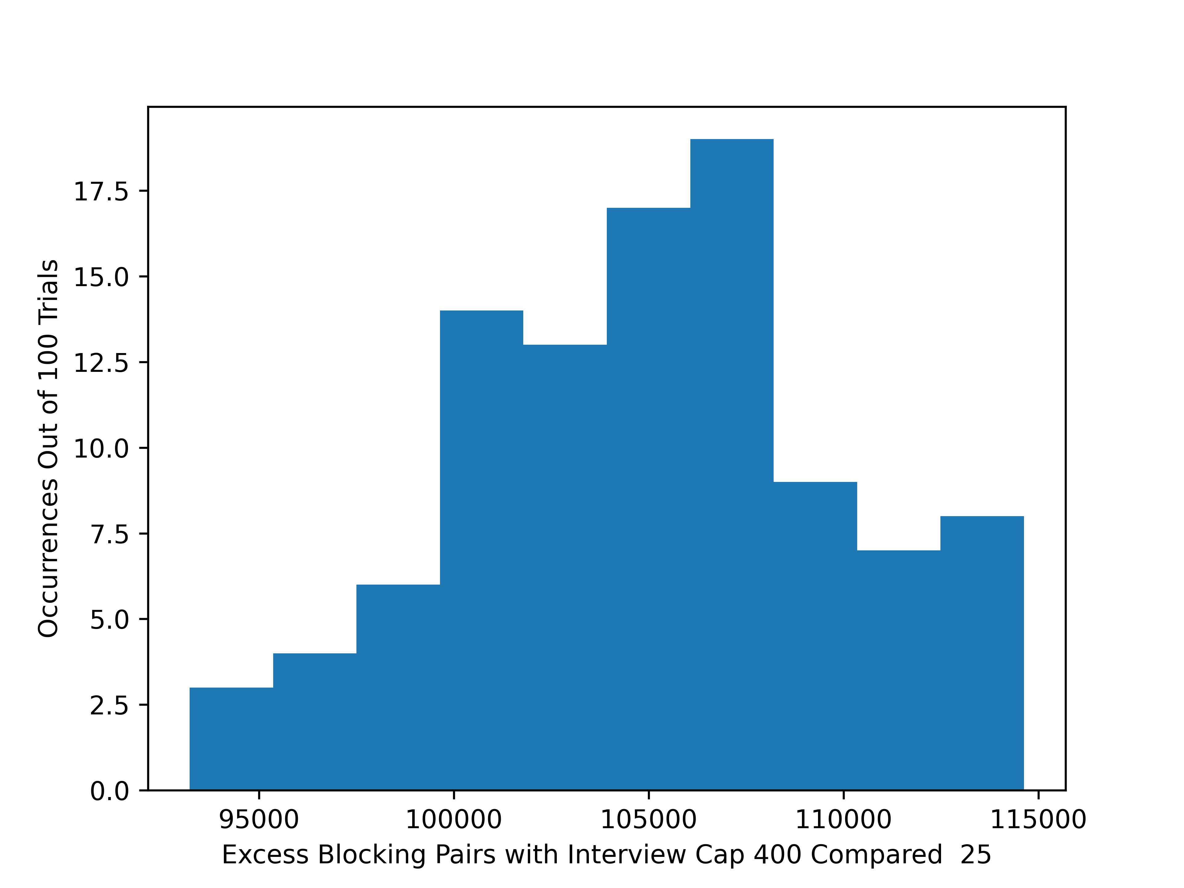
Figure 2(a) shows the distribution of the number of doctors who prefer their match under the optimal $k$ over the benchmark as well as the distribution of those with the opposite preference. We see that the former is considerably higher than the latter. Theorem 1 allows for certain unmatched doctors to gain from relaxing this policy. However, Figure 2(a) shows that such doctors are rare: on average, only 0.17 doctors gain while 334.45 are harmed. Figure 2(b) shows the same distributions, except for hospitals. Despite the fact that Theorem 1 does not address hospitals’ welfare, our simulations show that more hospitals prefer the optimal cap of $k=l$ than leaving the doctors unconstrained. The policy also has the benefit bringing stability to the final matching. Figure 2(c) shows the distribution of the increase in the number of blocking pairs when we go from the policy of $k=l$ to doctors being unconstrained. Finally, we compare the distribution of interviews among the doctors between the two capacity profiles in Figure 2(d). The constraint limiting doctors to $k=l$ interviews binds for many doctors. One implication is that significantly more doctors receive zero interviews when they are unconstrained. This is consistent with the intuition that if interviews were costless for doctors, then highly sought after doctors would hoard interviews and others would be left with nothing.

In our last simulations , we consider the possibility that the NRMP could set not only a cap on interviews that doctors can accept, but can also control the number of interviews that hospitals offer. From Proposition 2, we know that if preferences are common, the match rate would be maximized where $k=l$ . Figure 3 shows that, even when preferences are not exactly common, this is still the optimal policy: along the diagonal, where $k$ and $l$ are equal, the match rate is close to 100% and the match is almost stable.

In Appendix D, we modify our model to consist of two tiers of doctors and contrast simulations under naïve choices by hospitals (as above) to those under a heuristic for hospitals where every choice involves a “safety” doctor from the lower tier. The only qualitative difference is in the match rate: rather than being unmatched, hospitals match with safety candidates. The welfare based comparisons are very similar.

6 Conclusion

The COVID-19 pandemic has had a significant impact on the way interviews are conducted. It has also impacted the distribution of interviews among doctors. Through our theoretical results and simulations, we argue that the 2021 NRMP Match was likely inferior to previous years.

In future years, the NRMP should consider policies to mitigate these effects. Our analysis supports the idea of interview caps and our simulations provide evidence that such a policy would reduce the bottleneck created by the interview phase. Such caps can be implemented with very limited centralization, for instance, using a ticket system.

Even if such interventions are not possible in the very short run, our policy prescription is that residency programs should be advised to increase the number of candidates they interview relative to previous years.

Design of a fully centralized clearinghouse for interviews is an area that remains open. As earlier work on the interview pre-markets have shown, strategic analysis is only tractable under very stringent assumptions (Kadam 2021; Lee and Schwarz 2017; Beyhaghi 2019). Nonetheless, the current paper adds to the evidence (along with Echenique et al. 2020) that a more holistic approach that includes the interview stage is critical.

This interview-driven bottleneck is likely a factor in other matching contexts as well, including fully decentralized labor markets. For example, we expect it will affect the junior market for economists. This labor market typically consists of short interviews followed by on-campus visits. Physical constraints typically limit both the number of short interviews and on-campus visits a candidate is able to accept. With virtual interviews and virtual “fly-outs,” we expect candidates to accept more of both than they would otherwise. As a result, we could expect the same bottleneck in the economics job market as in the NRMP match.

References

(1)
Agarwal (2015) Agarwal, Nikhil (2015) “An Empirical Model of the Medical Match,” American Economic Review, Vol. 105, No. 7, pp. 1939–78, July.
Ali and Shorrer (2021) Ali, S Nageeb and Ran I Shorrer (2021) “The College Portfolio Problem,” working paper, Penn State.
Ashlagi et al. (2017) Ashlagi, Itai, Yash Kanoria, and Jacob D. Leshno (2017) “Unbalanced Random Matching Markets: The Stark Effect of Competition,” Journal of Political Economy, Vol. 125, No. 1, pp. 69–98.
Beyhaghi (2019) Beyhaghi, Hedyeh (2019) “Approximately-optimal Mechanisms in Auction Design, Search Theory, and Matching Markets,” Ph.D. dissertation, Cornell University. Chapter 5: Two-Sided Matching with Limited Number of Interviews.
Chade and Smith (2006) Chade, Hector and Lones Smith (2006) “Simultaneous Search,” Econometrica, Vol. 74, No. 5, pp. 1293–1307.
Echenique et al. (2020) Echenique, Federico, Ruy Gonzalez, Alistair Wilson, and Leeat Yariv (2020) “Top of the Batch: Interviews and the Match.”
Gale and Shapley (1962) Gale, David and Lloyd Shapley (1962) “College Admissions and the Stability of Marriage,” American Mathematical Monthly, Vol. 69, pp. 9–15.
Hitsch et al. (2010) Hitsch, Gunter J., Ali Hortaçsu, and Dan Ariely (2010) “Matching and Sorting in Online Dating,” American Economic Review, Vol. 100, No. 1, pp. 130–63, March.
Kadam (2021) Kadam, Sangram V (2021) “Interviewing in Matching Markets with Virtual Interviews.”
Lee (2017) Lee, SangMok (2017) “Incentive Compatibility of Large Centralized Matching Markets,” The Review of Economic Studies, Vol. 84, No. 1, pp. 444–463, 09.
Lee and Schwarz (2017) Lee, Robin S. and Michael Schwarz (2017) “Interviewing in two-sided matching markets,” The RAND Journal of Economics, Vol. 48, No. 3, pp. 835–855.
Morgan et al. (2020) Morgan, Helen Kang, Abigail F Winkel, Taylor Standiford, Rodrigo Muñoz, Eric A Strand, David A Marzano, Tony Ogburn, Carol A Major, Susan Cox, and Maya M Hammoud (2020) “The Case for Capping Residency Interviews,” Journal of Surgical Education, Vol. 78, No. 3, pp. 755–762, 09.
Rees-Jones (2018) Rees-Jones, Alex (2018) “Suboptimal behavior in strategy-proof mechanisms: Evidence from the residency match,” Games and Economic Behavior, Vol. 108, pp. 317–330.
Roth and Peranson (1999) Roth, Alvin E. and Elliott Peranson (1999) “The Redesign of the Matching Market for American Physicians: Some Engineering Aspects of Economic Design,” American Economic Review, Vol. 89, No. 4, pp. 748–780, September.
Roth and Sotomayor (1990) Roth, Alvin E. and Marilda A. Oliveira Sotomayor (1990) Two-Sided Matching: A Study in Game-Theoretic Modeling and Analysis, Econometric Society Monographs: Cambridge University Press.

Appendix A Role of Interviews: Preference Formation and Coordination

The interviews that precede the NRMP match serve at least two important purposes. The more obvious one is preference formation: while agents have a prior sense of their preferences, they update their preferences based on information revealed by the interviews. Less obvious is the coordination of whom to rank. A pair of agents can only be matched if they rank one another. In a market with hundreds, if not thousands, of potential partners, even formulating—much less submitting—a ranking of all possible partners is impractical. Thus agents submit only a portion of their preferences. Interviews function as a device to coordinate which portions they submit.

The second role of interviews that we have mentioned above is important even in a world where interviews are completely uninformative.

A natural question is to ask how the analysis of this paper is affected when we take preference formation into account. We first observe that we have drawn conclusions about doctors’ welfare (Theorem 1) and stability (Proposition 2 and Proposition 3). These comparisons are based on exogenous preferences. If preference formation is part of the model, then preferences are endogenous and there is no basis for such comparisons. However, we explain below how even here the match rate, which is an objective measure, is maximized when there is balance between the two sides’ interview capacities.

Represent the preferences of the agents prior to the interviews by the pre-interview preferences, $\overline{P}$ $\in\mathcal{P}$ . As with Propositions 2 and 3, we assume that $\overline{P}$ has common preferences.

Given an interview matching $\nu$ , for each agent $i\in D\cup H$ , let $P_{i}^{\nu}$ be $i$ ’s post-interview preferences. These are the preferences that $i$ forms through the interview process. The only requirement for $P^{\nu}_{i}$ is that $\nu(i)$ is the set of partners that $i$ ranks as acceptable. We do not make any other assumptions about how $P^{\nu}$ relates to $\overline{P}$ . In fact, we leave the exact orderings unspecified as this is unnecessary to draw conclusions about the match rate.

Since the pre-interview preferences are common, there is a unique interview matching, $\nu$ , that is stable with respect to these preferences. Given $\nu$ , unlike the two-phase process in Section 2, the next step is to use the post-interview preferences, $P^{\nu}$ (as opposed to $(\overline{P}_{i}|_{\nu(i)})_{i\in D\cup H}$ ) as the input to the doctor-proposing DA algorithm. The output is what we call the $(l,k)$ -matching with updating.

If the interviews either lead to a matching ( $l=k=1$ ) or do not impose any constraints ( $l,k\geq\min\{|D|,|H|\}$ ), then a total of $\min\{|D|,|H|\}$ pairs form. In the proof of Proposition 4 below, we demonstrate that when $l=k$ , the $(l,k)$ -matching with updating matches as many pairs as this “first best” benchmark. Increasing the gap between $l$ and $k$ causes the $(l,k)$ -matching with updating to fall short of this benchmark regardless of what the updated preferences are. This is a straightforward application of the pigeon hole principle.

Proposition 4.

Fix the hospitals’ interview capacity at $l$ and consider $k$ and $k^{\prime}$ such that either $k^{\prime}<k\leq l$ or $l\leq k<k^{\prime}$ . The $(l,k^{\prime})$ -matching with updating has a weakly lower match rate than the $(l,k)$ -matching with updating.

Proof.

Let $m=\min\left\{\left\lfloor\frac{|H|}{k}\right\rfloor,\left\lfloor\frac{|D|}{l}\right\rfloor\right\}$ . For each $n=1,\dots,m$ , let

	$\displaystyle D_{n}$	$\displaystyle=\{d_{t}:(n-1)l<t\leq nl\}$
		and
	$\displaystyle H_{n}$	$\displaystyle=\{h_{t}:(n-1)k<t\leq nk\}.$

By definition of $m$ , either $|D|<(m+1)l$ or $|H|<(m+1)k$ . Let $t_{D}=\min\{|D|,(m+1)l\}$ , $t_{H}=\min\{|H|,(m+1)k\}$ ,

	$\displaystyle D_{m+1}$	$\displaystyle=\left\{d_{t}:ml<t\leq t_{D}\right\},$
		and
	$\displaystyle H_{m+1}$	$\displaystyle=\left\{h_{t}:mk<t\leq t_{H}\right\}$

The unique pairwise stable interview matching, $\nu$ , is such that for each $n=1,\dots,m+1$ , every doctor in $D_{n}$ is interviewed by every hospital in $H_{n}$ —that is, for each $d\in D_{n}$ , $\nu(d)=H_{n}$ and for each $h\in H_{n},\nu(h)=D_{n}$ . Moreover, every doctor or hospital not in one of these sets has no interviews—that is, if there is $d_{t}$ such that $t>t_{D}$ , then $\nu(d_{t})=\emptyset$ and if there is $h_{t}$ such that $t>t_{H}$ , then $\nu(h_{t})=\emptyset$ .

Now we consider the $(l,k)$ -matching with updating, $\mu$ . Having received no interviews, any doctor or hospital with index higher than $t_{D}$ or $t_{H}$ , respectively, is necessarily unmatched regardless of the post-interview preferences. Since each agent’s post-interview preferences only rank those agents in one’s interview matching as acceptable, for each $n=1,\dots,m+1$ , we have that

1.

for each $d\in D_{n}$ , $\mu(d)\in H_{n}\cup\{d\}$ and
2.

for each $h\in H_{n}$ , $\mu(h)\in D_{n}\cup\{h\}$ .

If $l<k$ , then for each $n=1,\dots,m$ , $|D_{n}|=l<k=|H_{n}|$ . So exactly $k-l$ hospitals in $H_{n}$ are unmatched. There are $m(k-l)$ such hospitals. If there are fewer hospitals in $H_{m+1}$ than doctors in $D_{m+1}$ , then $|H_{m+1}|-|D_{m+1}|$ additional hospitals are unmatched. That is, the number of unmatched hospitals among those in $H_{m+1}$ is $\max\{0,|H_{m+1}|-|D_{m+1}|\}=\max\{0,(t_{H}-mk)-(t_{D}-m_{l})\}=\max\{0,(t_{H}-t_{D})-m(k-l)\}$ . So the total number of unmatched hospitals is

m(k-l)+\max\{0,(t_{H}-t_{D})-m(k-l)\},

which is weakly increasing in $k$ .

If $k<l$ , then every hospital $h_{t}$ such that $t\leq mk$ is matched by $\mu$ . As when $l<k$ , $\max\{0,(t_{H}-t_{D})-m(k-l)\}$ hospitals among those in $H_{m+1}$ are unmatched by $\mu$ . Every hospital $h_{t}$ such that $t>t_{H}$ is also unmatched. Thus, the number of hospitals that $\mu$ leaves unmatched is $\max\{0,|H|-(mk+|D|-ml)\}=\max\{0,|H|-|D|+m(l-k)\}$ , which is weakly decreasing in $k$ . ∎

Proposition 4 shows that the bottleneck of imbalanced interview capacities occurs at the interview stage. In this sense, the preference formation role of interviews is orthogonal to our main point regarding the harm such imbalance causes.

Appendix B Doctor-optimal Interview Matching

The only difference between our model and that of Echenique et al. 2020 is that we suppose that the interview matching is hospital-optimal rather than doctor-optimal. Their modeling choice is natural for the question they ask as it gives each doctor her best stable set of interviews. Thus, their result that most doctors match with hospitals they rank highly can only be stronger for other interview matchings. For our analysis, the doctor-optimal interview matching does not have this natural appeal. To the contrary, hospital-proposing DA is a reasonable approximation of the interview matching process. Nonetheless, our results are not driven by this choice. The only proof that relies on this choice is that of Theorem 1. In this section, we show that the result holds even for the doctor-optimal interview matching followed by the doctor-optimal final matching. In what follows, we use the same terminology and notation as before, with the understanding that the interview matching is doctor-optimal.

As in the statement of the theorem, suppose that for each $d\in D$ , $\kappa_{d}\leq\kappa^{\prime}_{d}$ . We show below that the Lemmas 2 and 3 hold even with the change from the hospital-optimal interview matching to the doctor-optimal interview matching. The key is to establish that, in the interview phase, if a doctor $d$ is rejected by a hospital $h$ under capacities $\kappa$ , then $h$ rejects her under $\kappa^{\prime}$ as well. Given capacities $\bar{\kappa}$ , let $A_{d}(m;\bar{\kappa})$ be the hospitals that $d$ proposes to and $R_{d}(m;\bar{\kappa})$ be the hospitals that reject doctor $d$ by the end of round $m$ of the interview phase. We show that these sets are monotonic in $\overline{\kappa}$ .

Claim 3.

For any positive integer $m$ ,

	$\displaystyle R_{d}(m;\kappa)$	$\displaystyle\subseteq R_{d}(m;\kappa^{\prime})$
	$\displaystyle A_{d}(m;\kappa)$	$\displaystyle\subseteq A_{d}(m;\kappa^{\prime})$

Proof.

We proceed by induction on $m$ , the base case being $m=1$ . In the first round of the interview phase, each $d\in D$ proposes to her favorite hospitals up to her interview capacity. Since every doctor proposes to at least as many hospitals under $\kappa^{\prime}$ as under $\kappa$ , every hospital receives at least as many proposals under $\kappa^{\prime}$ as under $\kappa$ . Therefore, if a doctor $d$ is rejected by a hospital $h$ in the first round of the interview phase under $\kappa$ , she is also rejected by $h$ in the first round under $\kappa^{\prime}$ . Now consider a round $m>1$ of the interview phase and suppose for each doctor $d$ that $R_{d}(m-1;\kappa)\subseteq R_{d}(m-1;\kappa^{\prime})$ and $A_{d}(m-1;\kappa)\subseteq A_{d}(m-1;\kappa^{\prime})$ . In round $m$ , each $d\in D$ proposes to her favorite hospitals that have not yet rejected her up to her interviewing capacity. Under $\kappa$ , $d$ proposes to her $\kappa_{d}$ favorite hospitals in $H\setminus R_{d}(m-1;\kappa)$ . Under $\kappa^{\prime}$ , she proposes to her $\kappa^{\prime}_{d}$ favorite hospitals in $H\setminus R_{d}(m-1;\kappa^{\prime})$ . By the inductive hypothesis, $H\setminus R_{d}(m-1;\kappa^{\prime})\subseteq H\setminus R_{d}(m-1;\kappa)$ . Therefore, if $d$ proposes to $h$ under $\kappa$ , either she proposes to $h$ under $\kappa^{\prime}$ as well (she is choosing more hospitals from a smaller set of options) or she has already proposed to and has been rejected by $h$ under $\kappa^{\prime}$ . In either case, if $h\in A_{d}(m;\kappa)$ , then $h\in A_{d}(m;\kappa^{\prime})$ . Since each hospital $h$ receives more proposals but its capacity does not change, if $h$ rejects doctor $d$ under $\kappa$ , she also rejects doctor $d$ when choosing from a larger set of doctors who have proposed to it under $\kappa^{\prime}$ . Therefore, if $h\in R_{d}(m;\kappa)$ , then $h\in R_{d}(m;\kappa^{\prime})$ . ∎

We now explain how 3 implies that Lemmas 2 and 3 hold even when we switch to the doctor-optimal interview matching. Let $\nu$ and $\mu$ be the interview and final matchings respectively, under $(\iota,\kappa)$ . Similarly, let $\nu^{\prime}$ and $\mu^{\prime}$ be the interview and final matchings under $(\iota,\kappa^{\prime})$ .

Lemma 2 says that for each $d\in D$ , if $h\in\nu^{\prime}(d)\setminus\nu(d)$ , then $\mu(d)\mathrel{P_{d}}h$ . Given $\bar{\kappa}$ , let $R_{d}(\bar{\kappa})$ denote the set of hospitals that reject $d$ in any round of the interview phase under capacities $\bar{\kappa}$ . By 3, $R_{d}(\kappa)\subseteq R_{d}(\kappa^{\prime})$ . Under $\kappa$ , $\nu(d)$ consists of $d$ ’s $\kappa_{d}$ most preferred hospitals in $H\setminus R_{d}(\kappa)$ . That is, the $\kappa_{d}$ highest-ranked hospitals that did not reject her. Under $\kappa^{\prime}$ , $\nu^{\prime}(d)$ comprises $d$ ’s $\kappa^{\prime}_{d}$ most preferred hospitals in $H\setminus R_{d}(\kappa^{\prime})$ . As $H\setminus R_{d}(\kappa^{\prime})\subseteq H\setminus R_{d}(\kappa)$ , if $h^{\prime}\in\nu^{\prime}(d)\setminus\nu(d)$ , then for every $h\in\nu(d)$ , $h\mathrel{P}_{d}h^{\prime}$ . In words, since $d$ is interviewed by $h$ under $\kappa$ , she was not rejected by $h$ under $\kappa$ . As more hospitals rejected $d$ under $\kappa^{\prime}$ than under $\kappa$ , $h$ does not reject $d$ under $\kappa$ . Therefore, $d$ could have proposed to $h$ under $\kappa$ , but she chose not to. Therefore, by revealed preference, she prefers all hospitals in $\nu(d)$ to any of her “new” interviews under $\kappa^{\prime}$ (those in $\nu^{\prime}(h)\setminus\nu(h)$ ).

Lemma 3 said that if $d\in v^{\prime}(h)$ , $d^{\prime}\in v(h)$ , and $d^{\prime}\mathrel{P_{h}}d$ , then $d^{\prime}\in v^{\prime}(h)$ . By 3, $d^{\prime}$ proposes to at least as many hospitals in the interview phase under $\kappa^{\prime}$ as under $\kappa$ . Since $d^{\prime}$ proposes to $h$ under $\kappa$ , she also proposes to $h$ under $\kappa^{\prime}$ . Each hospital $h$ accepts its $\iota_{h}$ favorite applicants, so if it accepts $d$ , it must also accept $d^{\prime}$ .

Since Lemmas 2 and 3 hold, the remainder of the proof follows exactly as in Section 3.

Appendix C Choice Functions for Interview Phase

In the interview phase, we compute a many-to-many matching. However, each doctor and each hospital only ultimately matches to at most one other partner, and each has strict preferences over partners. This necessitates the definition of a choice function over sets of partners. Consistent with the assumption of non-strategic behavior with complete information, we focus on acceptant choice functions that are responsive to preferences over partners and constrained by interview capacity. That is, given $P\in\mathcal{P}$ ,

•

From the set $H^{\prime}\subseteq H$ , each $d\in D$ chooses the $\kappa_{d}$ best elements of $H^{\prime}$ according to $P_{d}$ :

C_{d}(H^{\prime})=\left\{\begin{array}[]{ll}\{h\in H^{\prime}:h\mathrel{P}_{d}d\}&\text{if }|\{h\in H^{\prime}:h\mathrel{P}_{d}d\}|\leq\kappa_{d}\text{ and}\\ \\ B\subseteq\{h\in H^{\prime}:h\mathrel{P}_{d}d\}&\text{such that }|B|=\kappa_{d}\text{ and for each }h\in B\\ &\text{and each }h^{\prime}\in H^{\prime}\setminus B,h\mathrel{P}_{d}h^{\prime}\text{ otherwise.}\end{array}\right.

•

From the set $D^{\prime}\subseteq D$ , each $h\in H$ chooses the $\kappa_{h}$ best elements of $D^{\prime}$ according to $P_{h}$ :

C_{h}(D^{\prime})=\left\{\begin{array}[]{ll}\{d\in D^{\prime}:d\mathrel{P}_{h}h\}&\text{if }|\{d\in D^{\prime}:d\mathrel{P}_{h}h\}|\leq\iota_{h}\text{ and}\\ \\ B\subseteq\{d\in D^{\prime}:d\mathrel{P}_{h}h\}&\text{such that }|B|=\iota_{h}\text{ and for each }d\in B\\ &\text{and each }d^{\prime}\in D^{\prime}\setminus B,d\mathrel{P}_{h}d^{\prime}\text{ otherwise.}\end{array}\right.

Appendix D Epilogue: What Actually Happened

The 2021 “Match Day”—the day the NRMP announces the results of the match—was on March 19. In the words of the NRMP President and CEO, Donna L. Lamb,

The application and recruitment cycle was upended as a result of the pandemic, yet the results of the Match continue to demonstrate strong and consistent outcomes for participants.²⁶²⁶ 26 NRMP Press Release dated March 19, 2021.

Indeed, contrary to our results, there was a 2.6 percent increase in PGY-1 positions filled.

In this section, we argue that there is reason to be skeptical about the claim that the 2021 match is “strong and consistent.” In particular, we contend that focusing on match rates leads one to miss an effect that is analogous to our results.

We have assumed that hospitals naïvely extend interview invitations to their most preferred doctors first and that these trickle down to less preferred doctors. However, hospitals are not naïve in practice and use heuristics.²⁷²⁷ 27 Optimal strategies depend critically on the probability of matching with a doctor conditional on interviewing her (Chade and Smith 2006). In our context, these probabilities are dependent not only on other hospitals’ preferences and strategies but also on the rest of the hospital’s own interview choices. It is implausible that hospitals have this information and that they then compute the optimal portfolio of doctors to interview. Most heuristics include an option that has a high match probability even if it is ranked relatively low.²⁸²⁸ 28 Even the optimal solution has this property when being unmatched is very unattractive relative to matching with lower ranked candidates (Chade and Smith 2006). We call these candidates “safety” candidates. When hospitals offer interviews in this way, an increase to $k$ increases the proportion of hospitals that match with their safety candidates rather than the number of unfilled positions. In other words, hospitals tend to match with lower ranked doctors, the likelihood of matching for higher tier candidates decreases, and the likelihood of matching for lower tier candidates increases.

The very limited information that the NRMP has published so far supports this conjecture. We do not have access to the actual preferences of residency programs, nor their submitted rankings. Yet, the reported interview and ranking patterns in the 2020 NRMP Program Director Survey reveal a systematic preference for MD Seniors (graduating students from US MD medical schools) over DO Seniors (graduating from US DO medical schools) as well as MD and DO Grads (those who have previously graduated from US medical schools but had not matched). Nonetheless, the proportion of positions filled by MD Seniors declined slightly while the proportions of positions filled by the latter three increased slightly.²⁹²⁹ 29 See the NRMP Reports for 2020 and 2021. This lends support to our hypothesis that more positions were filled by safety candidates.

In what follows, we consider a variation of our model and contrast the matching patterns generated by the naïve behavior and a particular heuristic. The goal is to demonstrate the above explanation of how increased matches to safety candidates may mask the effects of increased interview capacities.

The change to the model is that we separate the doctors into two tiers— $D_{1}$ and $D_{2}$ (so $D_{1}\cap D_{2}=\emptyset$ and $D_{1}\cup D_{2}=D$ )—such that every hospital prefers every doctor in $D_{1}$ to every doctor in $D_{2}$ . We achieve this change by adding $\beta+\gamma+10$ to $u_{h}(d)$ , as specified in Section 5, for each $d\in D_{1}$ . We have chosen $D_{1}$ such that $|D_{1}|=200$ .

To model behavior under the heuristic, we use the following choice functions for hospitals, as opposed to those defined in Appendix C. From a set $D^{\prime}\subseteq D$ , hospital $h\in H$ chooses a safety candidate from the second tier, if one is available, and fills the remaining slots by choosing the best options in $D^{\prime}$ . In order to ensure that the interview matching (the hospital-proposing Deferred Acceptance) algorithm terminates, hospitals do not reconsider tentatively accepted interview offers. Thus, the choice function is parameterized by the number of interview offers to be made—in each round of the algorithm, the number of doctors a hospital chooses is its interview capacity minus the number of tentatively accepted offers in the previous round. Thus, when the hospital’s preferences over the doctors are represented by $P_{h}$ it chooses $n$ doctors from $D^{\prime}\subset D$ as follows: If $D\subseteq D_{1}$ ,

C_{h}(n,D^{\prime})=\left\{\begin{array}[]{ll}\{d\in D^{\prime}:d\mathrel{P}_{h}h\}&\text{if }|\{d\in D^{\prime}:d\mathrel{P}_{h}h\}|\leq n\text{ and}\\ \\ B\subseteq\{d\in D^{\prime}:d\mathrel{P}_{h}h\}&\text{such that }|B|=n\text{ and for each }d\in B\\ &\text{and each }d^{\prime}\in D^{\prime}\setminus B,d\mathrel{P}_{h}d^{\prime}\text{ otherwise.}\end{array}\right.

Otherwise, let $d^{s}$ be chosen uniformly at random from $D^{\prime}\cap D_{2}$ .³⁰³⁰ 30 Hospitals randomize their safety choice $d^{s}$ to avoid overlap. Then,

C_{h}(n,D^{\prime})=\left\{\begin{array}[]{ll}\{d^{s}\}\cup\{d\in D^{\prime}:d\mathrel{P}_{h}h\}&\text{if }|\{d\in D^{\prime}\setminus\{d^{s}\}:d\mathrel{P}_{h}h\}|\leq n-1\text{ and}\\ \\ \{d^{S}\}\cup B&\text{where }B\subseteq\{d\in D^{\prime}\setminus\{d^{s}\}:d\mathrel{P}_{h}h\}\\ &\text{is such that }|B|=n-1\text{ and for each }d\in B\\ &\text{and each }d^{\prime}\in D^{\prime}\setminus(B\cup\{d^{s}\}),d\mathrel{P}_{h}d^{\prime}\\ &\text{otherwise.}\end{array}\right.

We first observe that under the heuristic, the effect that increasing $k$ has on the match rate all but disappears. In Figures 4(a) and 4(b) we show the effects for the naïve behavior and the heuristic respectively.³¹³¹ 31 All parameter values are the same as in Section 5.

The dramatic difference in the match rates is entirely accounted for by the number of positions that are filled by second tier candidates. In other words, matching with lower ranked candidates is the alternative to being unmatched. This is easily seen in the comparison between Figures 5(a) and 5(b).

Other than the match rate, the remaining patterns that we presented in Section 5 persist with our modified model under the heuristic for hospitals’ choices. Under the heuristic, lower ranked doctors who would be unmatched at lower $k$ gain from the misallocation of interviews among higher ranked doctors. Nonetheless, more doctors prefer the outcome under a cap of $k=l$ than prefer the benchmark with no cap as shown in Figure 6(a). As noted above, hospitals tend to match with lower ranked doctors and therefore tend to be worse off, as shown in Figure 6(b). The result, as before, is driven by interview hoarding, which can be seen from the comparison of interview distributions with a cap of $k=l$ and with no cap in Figure 6(c).

Appendix E Robustness of Simulations: Choice of Random Utility Model and Parameters

In Section 5, we have adopted the random utility model of Ashlagi et al. 2017. Moreover, we have presented our results for fixed parameter values: $\beta=40$ , $\gamma=20$ , $l=25$ , $|D|=470$ , and $|H|=400$ . In this appendix, we discuss the robustness of our findings with regards to these choices.

We start with the random utility model. A very natural alternative is that of Lee 2017, which is the model that Echenique et al. 2020 have adopted. This model does not include a fit component, so a doctor’s utility from being matched to a hospital is a convex combination of a common (across all doctors) value and an idiosyncratic (to that doctor) value. A hospital’s utility from being matched to a doctor is similarly comprised. Thus, each hospital $h\in H$ has a common component to its quality, $x_{h}^{C}$ , and each doctor has a common component to her quality, $x^{C}_{d}$ . Aside from this, for each doctor-hospital pair, $d$ and $h$ , $\varepsilon_{dh}$ is the idiosyncratic value that $d$ assigns to $h$ and $\varepsilon_{hd}$ is the idiosyncratic value that $h$ assigns to $d$ . Then, the utilities that $h$ and $d$ enjoy from being matched to one another are

\begin{array}[]{c}u_{h}(d)=\alpha x_{d}^{C}+(1-\alpha)\varepsilon_{hd}\\ \text{ and }\\ u_{d}(h)=\alpha x_{h}^{C}+(1-\alpha)\varepsilon_{dh},\end{array}

respectively.

The random variables $x_{h}^{C}$ , $x_{d}^{C}$ , $\varepsilon_{dh}$ , and $\varepsilon_{hd}$ are all independently drawn from the uniform distribution over $[0,1]$ . The coefficients $\alpha$ and $(1-\alpha)$ are weights on the common and idiosyncratic components, respectively.

To make an apples-to-apples comparison between the two models, we set $\gamma=0$ since the Lee 2017 model does not have a fit component. The remaining difference is the distribution of the idiosyncratic components: the standard logistic distribution in one and the uniform distribution over $[0,1]$ in the other. Though these distributions have different supports, we can relate the two models by considering, for each pair $d,d^{\prime}\in D$ and each $h\in H$ , the degree of correlation between $u_{d}(h)$ and $u_{d^{\prime}}(h)$ as given by the Pearson correlation coefficient.³²³² 32 Given the symmetry of both models, we could equivalently state this as the correlation between $u_{h}(d)$ and $u_{h^{\prime}}(d)$ for for each pair $h,h^{\prime}\in H$ and each $d\in D$ . For the Lee 2017 model with parameter $\alpha$ , it is $\nicefrac{{\alpha^{2}}}{{\alpha^{2}+(1-\alpha)^{2}}}$ . For the Ashlagi et al. 2017 model with parameter $\beta$ (and $\gamma=0$ ), it is $\nicefrac{{\beta^{2}}}{{\beta^{2}+(2\pi)^{2}}}$ . Thus, utilities have the same linear correlation in the two models when

\alpha=\frac{\beta}{\beta+2\pi}.

We display this relationship in Figure 7. The value of $40$ that we have chosen for $\beta$ in Section 5 corresponds to an $\alpha$ of $0.864$ .

Now consider $\gamma$ . The higher $\gamma$ is, the more aligned preferences are across the two sides of the market. However, comparing two doctors, when $\gamma>0$ , the further apart they are in terms of their fit component, the less correlated their utilities are. Thus, since $\nicefrac{{\beta^{2}}}{{\beta^{2}+(2\pi)^{2}}}$ is the correlation between the utilities of two doctors with the same fit component, it is an upper bound on the correlation between the preferences of any two doctors. Our chosen value of $\gamma$ is on the same order of magnitude as $\beta$ .

We intend for our simulation results to be suggestive of how the insights from our analytical results may extend beyond the assumptions that we make for the sake of tractability. To this end, none of the choices that we have made are critical in driving the effects we describe in Section 5. We consider each of these choices in turn and make this point by focusing on how the match rate responds to different values of $k$ as shown in Figure 1(a). In other words, we show how this relationship changes as we vary our model and parameter choices. In what follows, we vary only one choice at a time, leaving fixed the other parameters as in Section 5.

In Figure 8, we consider various values of $\alpha$ and use the Lee 2017 model. As long as there is at least moderate correlation in preferences, we observe the effect, albeit with varying magnitude. Indeed, as the correlation between utilities grows, the effect becomes stronger, eventually converging to the one described by Proposition 3 when $\alpha=1$ .

In Figure 9, we consider various combinations of $\beta$ and $\gamma$ . Again, as $\beta$ grows, the correlation in preferences increases and the effect becomes stronger. However, as discussed above, $\gamma>0$ has the effect of decreasing the correlation between utilities of agents on the same side on average. Consistent with this understanding, we see that for a fixed value of $\beta$ , the lower $\gamma$ is, the stronger the effect.

The next parameter we vary is the number of doctors. Recall that we fixed the number of hospitals at $400$ for the simulations reported in Section 5. In Figure 10, holding the number of hospitals constant, we vary the number of doctors. The effect that $k$ has on the match rate is consistent with the rest of our results.³³³³ 33 For the cases where there are fewer than $400$ doctors, the match rate is necessarily lower than 100%.

Keeping the ratio of hospitals to doctors the same, we next proportionally vary the size of the market in Figure 11. The magnitude of the effect increases very slightly with market size, but there is no other change.

Finally, we consider the value of $l$ that we have fixed at $25$ for the simulations in Section 5. The lesson of Proposition 3 that an optimal policy is to set $k=l$ holds regardless of $l$ (Figure 12(a)). However, the magnitude diminishes with $l$ as see in Figure 12(b). Notably, the match rate does decrease as $k$ becomes larger than $l$ .