跳到论文正文
W Papers独立论文阅读器 arXiv:2102.06363 论文正文 计算阅读时间 · 0%
引用这篇论文根据当前论文元数据生成,正式投稿前建议核对。


License: CC BY 4.0
arXiv:2102.06363v7 [cs.IT] 30 Aug 2022

New Distributed Source Encryption Framework

Yasutada Oohama and Bagus Santoso Affiliation: University of Electro-Communications, Tokyo, Japan
Email: {oohama,santoso.bagus}@uec.ac.jp
Abstract

We pose and investigate the distributed secure source coding based on the common key cryptosystem. This cryptosystem includes the secrecy amplification problem for distributed encrypted sources with correlated keys using post-encryption-compression, which was posed investigated by Santoso and Oohama. In this paper we propose a new security criterion which is more natural compared with the commonly used security criterion which is based on the upper-bound of mutual information between the plaintext and the ciphertext. Under this criterion, we establish the necessary and sufficient condition for the secure transmission of correlated sources.

I Introduction

In this paper we pose and investigate the distributed secure source coding based on the common key cryptosystem. This cryptosystem includes the secrecy amplification problem for distributed encrypted sources with correlated keys using post-encryption-compression (PEC), which was posed investigated by Santoso and Oohama in [1], [2].

In this paper we propose a new security criterion which is more natural compared with the commonly used security criterion based on the upper-bound of mutual information between the plaintext and the ciphertext. For the proposed new metric we prove its validity. Concretely we establish the following two results:

  • a)

    We prove that if the mutual information is zero, then the proposed criterion is strictly zero.

  • b)

    The proposed criterion depends only on the property of the cryptsystem, implying that this criterion is more natural than the widely-used security metric based mutual information.

For the proposed security criterion, the part a) is quite essential. Without this condition, the criterion is meaningless.

Under the proposed security criterion we prove the strong converse theorem. We further derive a sufficient condition to achieve security. This sufficient condition matches the necessary condition. In our previous works of Santoso and Oohama [1], [2], we have derived a sufficient condition under the security criterion measured by the mutual information. To derive the sufficient condition we use the coding scheme proposed by Santoso and Oohama. We obtain the same sufficient condition as that of Santoso and Oohama [1], [2] under more natural condition than the mutual information.

Our study in this paper has a closely related to several previous works on the PEC, e.g., Johnson et al.[3], Klinc et al. [4]. Our study also has a close connection with several previous works on the Shannon cipher system, e.g. [5], [6] [7].

II Secure Source Coding Problem

II-A Preliminaries

In this subsection, we show the basic notations and related consensus used in this paper.

Random Sources of Information and Keys: Let (X1,X2)(X_{1},X_{2}) be a pair of random variables from a finite set 𝒳1×𝒳2\mathcal{X}_{1}\times\mathcal{X}_{2}. Let {(X1,t,X2,t)}t=1∞\{(X_{1,t},X_{2,t})\}_{t=1}^{\infty} be a stationary discrete memoryless source (DMS) such that for each t=1,2,…t=1,2,\ldots, the pair (X1,t,X2,t)(X_{1,t},X_{2,t}) takes values in finite set 𝒳1×𝒳2\mathcal{X}_{1}\times\mathcal{X}_{2} and obeys the same distribution as that of (X1,X2)(X_{1},X_{2}) denoted by pX1​X2={pX1​X2​(x1,x2)}(x1,x2)∈𝒳1×𝒳2p_{X_{1}X_{2}}=\{p_{X_{1}X_{2}}(x_{1},x_{2})\}_{(x_{1},x_{2})\in\mathcal{X}_{1}\times\mathcal{X}_{2}}. The stationary DMS {(X1,t,X2,t)}t=1∞\{(X_{1,t},X_{2,t})\}_{t=1}^{\infty} is specified with pX1​X2p_{X_{1}X_{2}}. Also, let (K1,K2)(K_{1},K_{2}) be a pair of random variables taken from the same finite set 𝒳1×𝒳2\mathcal{X}_{1}\times\mathcal{X}_{2} representing the pair of keys used for encryption at two separate terminals, of which the detailed description will be presented later. Similarly, let {(K1,t,K2,t)}t=1∞\{(K_{1,t},K_{2,t})\}_{t=1}^{\infty} be a stationary discrete memoryless source such that for each t=1,2,…t=1,2,\ldots, the pair (K1,t,K2,t)(K_{1,t},K_{2,t}) takes values in finite set 𝒳1×𝒳2\mathcal{X}_{1}\times\mathcal{X}_{2} and obeys the same distribution as that of (K1,K2)(K_{1},K_{2}) denoted by pK1​K2={pK1​K2​(k1,k2)}(k1,k2)∈𝒳1×𝒳2p_{K_{1}K_{2}}=\{p_{K_{1}K_{2}}(k_{1},k_{2})\}_{(k_{1},k_{2})\in\mathcal{X}_{1}\times\mathcal{X}_{2}}. The stationary DMS {(K1,t,K2,t)}t=1∞\{(K_{1,t},K_{2,t})\}_{t=1}^{\infty} is specified with pK1​K2p_{K_{1}K_{2}}.

Random Variables and Sequences: We write the sequence of random variables with length nn from the information source as follows: 𝑿1:=X1,1X1,2⋯X1,n{{\mbox{\boldmath$X$}}_{1}}:=X_{1,1}X_{1,2}\cdots X_{1,n}, 𝑿2:=X2,1X2,2⋯X2,n{{\mbox{\boldmath$X$}}_{2}}:=X_{2,1}X_{2,2}\cdots X_{2,n}. Similarly, the strings with length nn of 𝒳1n\mathcal{X}_{1}^{n} and 𝒳2n\mathcal{X}_{2}^{n} are written as 𝒙1:=x1,1x1,2⋯x1,n∈𝒳1n{{\mbox{\boldmath$x$}}_{1}}:=x_{1,1}x_{1,2}\cdots x_{1,n}\in\mathcal{X}_{1}^{n} and 𝒙2:=x2,1x2,2⋯x2,n∈𝒳2n{{\mbox{\boldmath$x$}}_{2}}:=x_{2,1}x_{2,2}\cdots x_{2,n}\in\mathcal{X}_{2}^{n} respectively. For (𝒙1,𝒙2)∈𝒳1n×𝒳2n({{\mbox{\boldmath$x$}}_{1}},{{\mbox{\boldmath$x$}}_{2}})\in\mathcal{X}_{1}^{n}\times\mathcal{X}_{2}^{n}, p𝑿1​𝑿2​(𝒙1,𝒙2)p_{{{\mbox{\scriptsize\boldmath$X$}}_{1}}{{\mbox{\scriptsize\boldmath$X$}}_{2}}}({{\mbox{\boldmath$x$}}_{1}},{{\mbox{\boldmath$x$}}_{2}}) stands for the probability of the occurrence of (𝒙1,𝒙2)({{\mbox{\boldmath$x$}}_{1}},{{\mbox{\boldmath$x$}}_{2}}). When the information source is memoryless specified with pX1​X2p_{X_{1}X_{2}}, we have the following equation holds: p𝑿1​𝑿2​(𝒙1,𝒙2)=∏t=1npX1​X2​(x1,t,x2,t)p_{{{\mbox{\scriptsize\boldmath$X$}}_{1}}{{\mbox{\scriptsize\boldmath$X$}}_{2}}}({{\mbox{\boldmath$x$}}_{1}},{{\mbox{\boldmath$x$}}_{2}})=\prod_{t=1}^{n}p_{X_{1}X_{2}}(x_{1,t},x_{2,t}). In this case we write p𝑿1​𝑿2​(𝒙1,𝒙2)p_{{{\mbox{\scriptsize\boldmath$X$}}_{1}}{{\mbox{\scriptsize\boldmath$X$}}_{2}}}({{\mbox{\boldmath$x$}}_{1}},{{\mbox{\boldmath$x$}}_{2}}) as pX1​X2n​(𝒙1,𝒙2)p_{X_{1}X_{2}}^{n}({{\mbox{\boldmath$x$}}_{1}},{{\mbox{\boldmath$x$}}_{2}}). Similar notations are used for other random variables and sequences.

Consensus and Notations: Without loss of generality, throughout this paper, we assume that 𝒳1\mathcal{X}_{1} and 𝒳2\mathcal{X}_{2} are finite fields. The notation ⊕\oplus is used to denote the field addition operation, while the notation ⊖\ominus is used to denote the field subtraction operation, i.e., a⊖b=a⊕(−b)a\ominus b=a\oplus(-b) for any elements a,ba,b of a same finite field. For the sake of simplicity, we use the same notation for field addition and subtraction for both 𝒳1\mathcal{X}_{1} and 𝒳2\mathcal{X}_{2}. Throughout this paper all logarithms are taken to the base 2.

II-B Basic System Description

First, let the information sources and keys be generated independently by different parties 𝒮𝗀𝖾𝗇\mathcal{S}_{\mathsf{gen}} and 𝒦𝗀𝖾𝗇\mathcal{K}_{\mathsf{gen}} respectively. In our setting, we assume the followings.

  • •

    The random keys 𝑲1{{\mbox{\boldmath$K$}}_{1}} and 𝑲2{{\mbox{\boldmath$K$}}_{2}} are generated by 𝒦𝗀𝖾𝗇\mathcal{K}_{\mathsf{gen}}.

  • •

    The key 𝑲1{{\mbox{\boldmath$K$}}_{1}} is correlated to 𝑲2{{\mbox{\boldmath$K$}}_{2}}.

  • •

    The sources 𝑿1{{\mbox{\boldmath$X$}}_{1}} and 𝑿2{{\mbox{\boldmath$X$}}_{2}} are generated by 𝒮𝗀𝖾𝗇\mathcal{S}_{\mathsf{gen}} and are correlated to each other.

  • •

    The sources are independent to the keys.

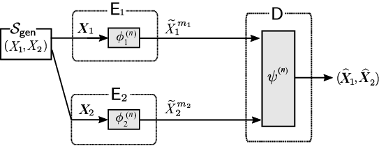
Source coding without encryption: The two correlated random sources 𝐗1{{\mbox{\boldmath$X$}}_{1}} and 𝐗2{{\mbox{\boldmath$X$}}_{2}} from 𝒮𝗀𝖾𝗇\mathcal{S}_{\mathsf{gen}} be sent to two separated nodes 𝖤1\mathsf{E}_{1} and 𝖤2\mathsf{E}_{2} respectively. Further settings of the system are described as follows. Those are also shown in Fig. 1.

  1. 1.

    Encoding Process: For each i=1,2i=1,2, at the node 𝖤i\mathsf{E}_{i}, the encoder function ϕi(n):𝒳in\phi_{i}^{(n)}:{\cal X}_{i}^{n} →𝒳imi\to{\cal X}_{i}^{m_{i}} observes 𝑿i{{\mbox{\boldmath$X$}}_{i}} to generate X~imi=ϕi(n)​(𝑿i)\tilde{X}_{i}^{m_{i}}=\phi_{i}^{(n)}({{\mbox{\boldmath$X$}}_{i}}). Without loss of generality we may assume that ϕi(n)\phi_{i}^{(n)} is surjective.

  2. 2.

    Transmission: Next, the encoded sources X~imi\tilde{X}_{i}^{m_{i}}, i=1,2i=1,2 are sent to the information processing center 𝖣\mathsf{D} through two noiseless channels.

  3. 3.

    Decoding Process: In 𝖣\mathsf{D}, the decoder function observes X~mi,i=1,2\tilde{X}^{m_{i}},i=1,2 to output (𝑿^1,𝑿^2)(\widehat{{\mbox{\boldmath$X$}}}_{1},\widehat{{\mbox{\boldmath$X$}}}_{2}), using the one-to-one mapping ψ(n)\psi^{(n)} defined by ψ(n):𝒳1m1×𝒳2m2→𝒳1n×𝒳2n\psi^{(n)}:{\cal X}_{1}^{m_{1}}\times{\cal X}_{2}^{m_{2}}\to{\cal X}_{1}^{n}\times{\cal X}_{2}^{n}. Here we set

    (𝑿^1,𝑿^2):=\displaystyle(\widehat{{\mbox{\boldmath$X$}}}_{1},\widehat{{\mbox{\boldmath$X$}}}_{2}):= ψ(n)​(X~1m1,X~2m2)\displaystyle\psi^{(n)}(\tilde{X}^{m_{1}}_{1},\tilde{X}^{m_{2}}_{2})
    =\displaystyle= ψ(n)​(ϕ1(n)​(𝑿1),ϕ2(n)​(𝑿2)).\displaystyle\psi^{(n)}\left(\phi^{(n)}_{1}({\mbox{\boldmath$X$}}_{1}),\phi^{(n)}_{2}({\mbox{\boldmath$X$}}_{2})\right).

    More concretely, the decoder outputs the unique pair (𝑿^1,𝑿^2)(\widehat{{\mbox{\boldmath$X$}}}_{1},\widehat{{\mbox{\boldmath$X$}}}_{2}) from (ϕ1(n))−1​(X~1m1)×(ϕ2(n))−1​(X~2m2)(\phi_{1}^{(n)})^{-1}(\tilde{X}_{1}^{m_{1}})\times(\phi_{2}^{(n)})^{-1}(\tilde{X}_{2}^{m_{2}}) in a proper manner.

Refer to caption
Fig. 1: Distributed source coding without encryption.
Refer to caption
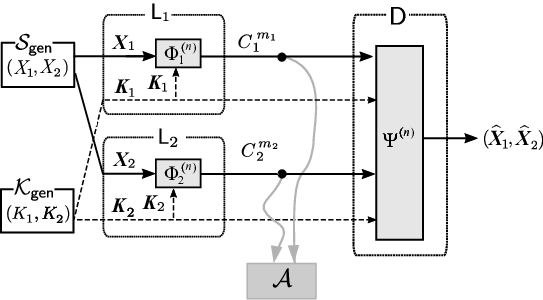
Fig. 2: Distributed source coding with encryption.

For the above (ϕ1(n),ϕ2(n),ψ(n))(\phi_{1}^{(n)},\phi_{2}^{(n)},\psi^{(n)}), we define the set 𝒟(n)\mathcal{D}^{(n)} of correct decoding by

𝒟(n)\displaystyle\mathcal{D}^{(n)} :={(𝒙1,𝒙2)∈𝒳1n×𝒳2n:\displaystyle:=\{({\mbox{\boldmath$x$}}_{1},{\mbox{\boldmath$x$}}_{2})\in\mathcal{X}_{1}^{n}\times\mathcal{X}_{2}^{n}:
ψ(n)(φ1(n)(𝒙1),φ2(n)(𝒙2))=(𝒙1,𝒙2)}.\displaystyle\psi^{(n)}(\varphi_{1}^{(n)}({\mbox{\boldmath$x$}}_{1}),\varphi_{2}^{(n)}({\mbox{\boldmath$x$}}_{2}))=({\mbox{\boldmath$x$}}_{1},{\mbox{\boldmath$x$}}_{2})\}.

On |𝒟(n)||{\cal D}^{(n)}|, we have the following property.

Property 1

We have the following.

|𝒟(n)|=|𝒳1m1|​|𝒳2m2|.\displaystyle|{\cal D}^{(n)}|=|{\cal X}_{1}^{m_{1}}||{\cal X}_{2}^{m_{2}}|. (1)

Proof of Property 1 is given in Appendix -A.

Remark 1

In brief, the reason that we can assume the decoder as injective mapping without loss of generality is that for any non-injective decoder, we can construct an injective decoder with the same performance. More concretely, for any encoder ϕ~(n):𝒳in→𝒳imi,i=1,2\tilde{\phi}^{(n)}:\mathcal{X}_{i}^{n}\rightarrow\mathcal{X}_{i}^{m_{i}},i=1,2 and any ψ~(n)\tilde{\psi}^{(n)} not necessary injective, there exists (ϕ1(n),ϕ2(n),ψ(n))(\phi_{1}^{(n)},\phi_{2}^{(n)},\psi^{(n)}) where ψ(n)\psi^{(n)} is injective such that the following holds: ψ~(n)​(ϕ~1​(𝒳1n),ϕ~2​(𝒳2n))=ψ(n)​(ϕ1​(𝒳1n),ϕ2​(𝒳2n))\tilde{\psi}^{(n)}(\tilde{\phi}_{1}({\cal X}_{1}^{n}),\tilde{\phi}_{2}({\cal X}_{2}^{n}))=\psi^{(n)}(\phi_{1}({\cal X}_{1}^{n}),\phi_{2}({\cal X}_{2}^{n})), |ϕ~i(𝒳in)|≥|ϕi(𝒳in)|,i=1,2|\tilde{\phi}_{i}({\cal X}_{i}^{n})|\geq|{\phi}_{i}({\cal X}_{i}^{n})|,i=1,2.

Distributed source coding with encryption:

The two correlated random sources 𝐗1{{\mbox{\boldmath$X$}}_{1}} and 𝐗2{{\mbox{\boldmath$X$}}_{2}} from 𝒮𝗀𝖾𝗇\mathcal{S}_{\mathsf{gen}} are sent to two separated nodes 𝖫1\mathsf{L}_{1} and 𝖫2\mathsf{L}_{2}, respectively. The two random keys 𝐊1{{\mbox{\boldmath$K$}}_{1}} and 𝐊2{{\mbox{\boldmath$K$}}_{2}} from 𝒦𝗀𝖾𝗇\mathcal{K}_{\mathsf{gen}}, are also sent to 𝖫1\mathsf{L}_{1} and and 𝖫2\mathsf{L}_{2}, respectively. Further settings of our system are described as follows. Those are also shown in Fig. 2.

  1. 1.

    Source Processing: For each i=1,2i=1,2, at the node 𝖫i\mathsf{L}_{i}, 𝑿i{{\mbox{\boldmath$X$}}}_{i} is encrypted with the key 𝑲i{{\mbox{\boldmath$K$}}}_{i} using the encryption function Φi(n):𝒳in×𝒳in\Phi_{i}^{(n)}:{\cal X}_{i}^{n}\times{\cal X}_{i}^{n} →𝒳imi\to{\cal X}_{i}^{m_{i}}. For each i=1,2i=1,2, the ciphertext CimiC_{i}^{m_{i}} of 𝑿i{{\mbox{\boldmath$X$}}}_{i} is given by Cimi=Φi(n)​(𝑲i,𝑿i)C_{i}^{m_{i}}=\Phi_{i}^{(n)}({{\mbox{\boldmath$K$}}}_{i},{{\mbox{\boldmath$X$}}}_{i}). On the encryption function Φi(n),i=1,2\Phi_{i}^{(n)},i=1,2, we use the folloiwng notation:

    Φi(n)​(𝑲i,𝑿i)=Φi,𝑲i(n)​(𝑿i)=Φi,𝑿i(n)​(𝑲i).\Phi_{i}^{(n)}({{\mbox{\boldmath$K$}}}_{i},{{\mbox{\boldmath$X$}}}_{i})=\Phi^{(n)}_{i,{{\mbox{\scriptsize\boldmath$K$}}}_{i}}({{\mbox{\boldmath$X$}}}_{i})=\Phi^{(n)}_{i,{{\mbox{\scriptsize\boldmath$X$}}}_{i}}({{\mbox{\boldmath$K$}}}_{i}).
  2. 2.

    Transmission: Next, the ciphertext Cimi,i=1,2C_{i}^{m_{i}},i=1,2 are sent to the information processing center 𝖣\mathsf{D} through two public communication channels. Meanwhile, the key 𝑲i,i=1,2{{\mbox{\boldmath$K$}}}_{i},i=1,2, are sent to 𝖣\mathsf{D} through two private communication channels.

  3. 3.

    Sink Node Processing: In 𝖣\mathsf{D}, we decrypt the ciphertext (𝑿^1,𝑿^2)(\widehat{{\mbox{\boldmath$X$}}}_{1},\widehat{{\mbox{\boldmath$X$}}}_{2}) from Cimi,i=1,2,C_{i}^{m_{i}},i=1,2, using the key 𝑲i,i=1,2{{\mbox{\boldmath$K$}}}_{i},i=1,2, through the corresponding decryption procedure Ψ(n)\Psi^{(n)} defined by Ψ(n):𝒳1n×𝒳2n×𝒳1m1×𝒳2m2→𝒳1n×𝒳2n.\Psi^{(n)}:{\cal X}_{1}^{n}\times{\cal X}_{2}^{n}\times{\cal X}_{1}^{m_{1}}\times{\cal X}_{2}^{m_{2}}\to{\cal X}_{1}^{n}\times{\cal X}_{2}^{n}. Here we set

    (𝑿^1,𝑿^2):=Ψ(n)​(𝑲1,𝑲2,C1m1,C2m2).(\widehat{{\mbox{\boldmath$X$}}}_{1},\widehat{{\mbox{\boldmath$X$}}}_{2}):=\Psi^{(n)}({{\mbox{\boldmath$K$}}_{1}},{{\mbox{\boldmath$K$}}_{2}},C_{1}^{m_{1}},C_{2}^{m_{2}}).

    More concretely, the decoder outputs the unique pair (𝑿^1,𝑿^2)(\widehat{{\mbox{\boldmath$X$}}}_{1},\widehat{{\mbox{\boldmath$X$}}}_{2}) from (Φ1,𝑲1(n))−1​(C1m1)×(Φ2,𝑲1(n))−1​(C2m2)(\Phi_{1,{\mbox{\scriptsize\boldmath$K$}}_{1}}^{(n)})^{-1}({C}_{1}^{m_{1}})\times(\Phi_{2,{\mbox{\scriptsize\boldmath$K$}}_{1}}^{(n)})^{-1}({C}_{2}^{m_{2}}) in a proper manner. On the decryption function Ψ(n)\Psi^{(n)}, we use the following notation:

    Ψ(n)​(𝑲1,𝑲2,C1m1,C2m2)=Ψ𝑲1,𝑲2(n)​(C1m1,C2m2)\displaystyle\Psi^{(n)}({{\mbox{\boldmath$K$}}}_{1},{{\mbox{\boldmath$K$}}}_{2},C_{1}^{m_{1}},C_{2}^{m_{2}})=\Psi^{(n)}_{{\mbox{\scriptsize\boldmath$K$}}_{1},{\mbox{\scriptsize\boldmath$K$}}_{2}}(C_{1}^{m_{1}},C_{2}^{m_{2}})
    =ΨC1m1,C2m2(n)​(𝑲1,𝑲2).\displaystyle=\Psi^{(n)}_{C_{1}^{m_{1}},C_{2}^{m_{2}}}({{\mbox{\boldmath$K$}}_{1}},{{\mbox{\boldmath$K$}}_{2}}).

Fix any (𝐊1,𝐊2)=(𝐤1,𝐤2)∈𝒳1n×𝒳2n({\mbox{\boldmath$K$}}_{1},{\mbox{\boldmath$K$}}_{2})=({\mbox{\boldmath$k$}}_{1},{\mbox{\boldmath$k$}}_{2})\in\mathcal{X}_{1}^{n}\times\mathcal{X}_{2}^{n}. For this (𝐊1,𝐊2)({\mbox{\boldmath$K$}}_{1},{\mbox{\boldmath$K$}}_{2}) and for (Φ1(n),Φ2(n),Ψ(n))(\Phi_{1}^{(n)},\Phi_{2}^{(n)},\Psi^{(n)}), we define the set 𝒟𝐤1,𝐤2(n)\mathcal{D}^{(n)}_{{\mbox{\scriptsize\boldmath$k$}}_{1},{\mbox{\scriptsize\boldmath$k$}}_{2}} of correct decoding by

𝒟𝒌1,𝒌2(n)\displaystyle\mathcal{D}^{(n)}_{{\mbox{\scriptsize\boldmath$k$}}_{1},{\mbox{\scriptsize\boldmath$k$}}_{2}} :={(𝒙1,𝒙2)∈𝒳1n×𝒳2n:\displaystyle:=\{({\mbox{\boldmath$x$}}_{1},{\mbox{\boldmath$x$}}_{2})\in\mathcal{X}_{1}^{n}\times\mathcal{X}_{2}^{n}:
Ψ(n)(Φ1(n)(𝒌1,𝒙1),(Φ2(n)(𝒌2,𝒙2))=(𝒙1,𝒙2)}.\displaystyle\Psi^{(n)}(\Phi_{1}^{(n)}({\mbox{\boldmath$k$}}_{1},{\mbox{\boldmath$x$}}_{1}),(\Phi_{2}^{(n)}({\mbox{\boldmath$k$}}_{2},{\mbox{\boldmath$x$}}_{2}))=({\mbox{\boldmath$x$}}_{1},{\mbox{\boldmath$x$}}_{2})\}.

We require that the cryptosystem (Φ1(n),Φ2(n),Ψ(n))(\Phi_{1}^{(n)},\Phi_{2}^{(n)},\Psi^{(n)}) must satisfy the following condition.

Condition: For each distributed source encryption sysytem (Φ1(n),Φ2(n),Ψ(n))(\Phi_{1}^{(n)},\Phi_{2}^{(n)},\Psi^{(n)}), there exists a distributed source coding system (ϕ1(n),ϕ2(n),ψ(n))(\phi_{1}^{(n)},\phi_{2}^{(n)},\psi^{(n)}) such that for any (𝐤1,𝐤2)∈𝒳1n×𝒳2n({\mbox{\boldmath$k$}}_{1},{\mbox{\boldmath$k$}}_{2})\in\mathcal{X}_{1}^{n}\times\mathcal{X}_{2}^{n} and for any (𝐱1,𝐱2)∈𝒳1n×𝒳2n({\mbox{\boldmath$x$}}_{1},{\mbox{\boldmath$x$}}_{2})\in\mathcal{X}_{1}^{n}\times\mathcal{X}_{2}^{n},

Ψ𝒌1,𝒌2(n)​(Φ1,𝒌1(n)​(𝒙1),Φ2,𝒌2(n)​(𝒙2))\displaystyle\Psi_{{\mbox{\scriptsize\boldmath$k$}}_{1},{\mbox{\scriptsize\boldmath$k$}}_{2}}^{(n)}(\Phi_{1,{\mbox{\scriptsize\boldmath$k$}}_{1}}^{(n)}({\mbox{\boldmath$x$}}_{1}),\Phi_{2,{\mbox{\scriptsize\boldmath$k$}}_{2}}^{(n)}({\mbox{\boldmath$x$}}_{2}))
=ψ(n)​(ϕ1(n)​(𝒙1),ϕ2(n)​(𝒙2)).\displaystyle=\psi^{(n)}(\phi_{1}^{(n)}({\mbox{\boldmath$x$}}_{1}),\phi_{2}^{(n)}({\mbox{\boldmath$x$}}_{2})).

The above condition implies that

𝒟(n)=𝒟𝒌1,𝒌2(n),∀(𝒌1,𝒌2)∈𝒳1n×𝒳2n.{\cal D}^{(n)}={\cal D}^{(n)}_{{\mbox{\scriptsize\boldmath$k$}}_{1},{\mbox{\scriptsize\boldmath$k$}}_{2}},\forall({\mbox{\boldmath$k$}}_{1},{\mbox{\boldmath$k$}}_{2})\in{\cal X}_{1}^{n}\times{\cal X}_{2}^{n}.

We have the following properties on 𝒟(n){\cal D}^{(n)}.

Property 2
  • a)

    If (𝒙1,𝒙2),(𝒙1′,𝒙2′)∈𝒟(n)({\mbox{\boldmath$x$}}_{1},{\mbox{\boldmath$x$}}_{2}),({\mbox{\boldmath$x$}}^{\prime}_{1},{\mbox{\boldmath$x$}}^{\prime}_{2})\in{\cal D}^{(n)} and (𝒙1,𝒙2)≠(𝒙1′,𝒙2′)({\mbox{\boldmath$x$}}_{1},{\mbox{\boldmath$x$}}_{2})\neq({\mbox{\boldmath$x$}}^{\prime}_{1},{\mbox{\boldmath$x$}}^{\prime}_{2}), then

    (Φ1,𝒌1(n)​(𝒙1),Φ2,𝒌2(n)​(𝒙2))≠(Φ1,𝒌1(n)​(𝒙1′),Φ2,𝒌2(n)​(𝒙2′)).(\Phi^{(n)}_{1,{\mbox{\scriptsize\boldmath$k$}}_{1}}({\mbox{\boldmath$x$}}_{1}),\Phi^{(n)}_{2,{\mbox{\scriptsize\boldmath$k$}}_{2}}({\mbox{\boldmath$x$}}_{2}))\neq(\Phi^{(n)}_{1,{\mbox{\scriptsize\boldmath$k$}}_{1}}({\mbox{\boldmath$x$}}^{\prime}_{1}),\Phi^{(n)}_{2,{\mbox{\scriptsize\boldmath$k$}}_{2}}({\mbox{\boldmath$x$}}^{\prime}_{2})).
  • b)

    ∀(𝒌1,𝒌2)\forall({\mbox{\boldmath$k$}}_{1},{\mbox{\boldmath$k$}}_{2}) and ∀(c1m1,c2m2)\forall(c_{1}^{m_{1}},c_{2}^{m_{2}}), ∃(𝒙1,𝒙2)\exists({\mbox{\boldmath$x$}}_{1},{\mbox{\boldmath$x$}}_{2}) ∈𝒟(n)\in{\cal D}^{(n)} such that

    (Φ1,𝒌1(n)​(𝒙1),Φ2,𝒌2(n)​(𝒙2))=(c1m1,c2m2).(\Phi^{(n)}_{1,{\mbox{\scriptsize\boldmath$k$}}_{1}}({\mbox{\boldmath$x$}}_{1}),\Phi^{(n)}_{2,{\mbox{\scriptsize\boldmath$k$}}_{2}}({\mbox{\boldmath$x$}}_{2}))=(c_{1}^{m_{1}},c_{2}^{m_{2}}).

Proof of Property 2 is given in Appendix -B. On the above distributed source encryption scheme, we have an important lemma. Before describing this lemma we give an observation on pC1m1​C2m2|𝐗1​𝐗2p_{C_{1}^{m_{1}}C_{2}^{m_{2}}|{\mbox{\scriptsize\boldmath$X$}}_{1}{\mbox{\scriptsize\boldmath$X$}}_{2}}. For (𝐱1,𝐱2)∈𝒳1n×𝒳2n({\mbox{\boldmath$x$}}_{1},{\mbox{\boldmath$x$}}_{2})\in{\cal X}_{1}^{n}\times{\cal X}_{2}^{n}, we set

𝒜𝒙1,𝒙2​(c1m1,c2m2)\displaystyle{\cal A}_{{\mbox{\scriptsize\boldmath$x$}}_{1},{\mbox{\scriptsize\boldmath$x$}}_{2}}(c_{1}^{m_{1}},c_{2}^{m_{2}})
:={(𝒌1,𝒌2):Φi,𝒙i(n)(𝒌i)=cimi,i=1,2}.\displaystyle:=\left\{({\mbox{\boldmath$k$}}_{1},{\mbox{\boldmath$k$}}_{2}):\Phi^{(n)}_{i,{\mbox{\scriptsize\boldmath$x$}}_{i}}({{\mbox{\boldmath$k$}}}_{i})=c_{i}^{m_{i}},i=1,2\right\}.

We have that for each (c1m1,c2m2,𝐱1,𝐱2)∈𝒳1m1×𝒳2m2×𝒳1n×𝒳2n(c_{1}^{m_{1}},c_{2}^{m_{2}},{\mbox{\boldmath$x$}}_{1},{\mbox{\boldmath$x$}}_{2})\in{\cal X}_{1}^{m_{1}}\times{\cal X}_{2}^{m_{2}}\times{\cal X}_{1}^{n}\times{\cal X}_{2}^{n},

pC1m1​C2m2|𝑿1​𝑿2(c1m1,c2m2|𝒙1,𝒙1)\displaystyle p_{C_{1}^{m_{1}}C_{2}^{m_{2}}|{\mbox{\scriptsize\boldmath$X$}}_{1}{\mbox{\scriptsize\boldmath$X$}}_{2}}(c_{1}^{m_{1}},c_{2}^{m_{2}}|{\mbox{\boldmath$x$}}_{1},{\mbox{\boldmath$x$}}_{1})
=Pr{(𝑲1,𝑲2)∈𝒜𝒙1,𝒙2(c1m1,c2m2)|𝑿1=𝒙1,𝑿2=𝒙2}\displaystyle={\rm Pr}\left\{({\mbox{\boldmath$K$}}_{1},{\mbox{\boldmath$K$}}_{2})\in{\cal A}_{{\mbox{\scriptsize\boldmath$x$}}_{1},{\mbox{\scriptsize\boldmath$x$}}_{2}}(c_{1}^{m_{1}},c_{2}^{m_{2}})\Bigl|{\mbox{\boldmath$X$}}_{1}={\mbox{\boldmath$x$}}_{1},{\mbox{\boldmath$X$}}_{2}={\mbox{\boldmath$x$}}_{2}\right\}
=(a)Pr{(𝑲1,𝑲2)∈𝒜𝒙1,𝒙2(c1m1,c2m2)}.\displaystyle\stackrel{{\scriptstyle{\rm(a)}}}{{=}}{\rm Pr}\left\{({\mbox{\boldmath$K$}}_{1},{\mbox{\boldmath$K$}}_{2})\in{\cal A}_{{\mbox{\scriptsize\boldmath$x$}}_{1},{\mbox{\scriptsize\boldmath$x$}}_{2}}(c_{1}^{m_{1}},c_{2}^{m_{2}})\right\}. (2)

Step (a) follows from (𝐊1,𝐊2)⟂(𝐗1,𝐗2)({\mbox{\boldmath$K$}}_{1},{\mbox{\boldmath$K$}}_{2})\perp({\mbox{\boldmath$X$}}_{1},{\mbox{\boldmath$X$}}_{2}). We can see from (14) that for each (𝐱1,𝐱2)∈𝒳1n×𝒳2n({\mbox{\boldmath$x$}}_{1},{\mbox{\boldmath$x$}}_{2})\in{\cal X}_{1}^{n}\times{\cal X}_{2}^{n}, the component pC1m1​C2m2|𝐗1​𝐗2​(c1m1,c2m2𝐶𝐿𝑂𝑆𝐸p_{C_{1}^{m_{1}}C_{2}^{m_{2}}|{\mbox{\scriptsize\boldmath$X$}}_{1}{\mbox{\scriptsize\boldmath$X$}}_{2}}(c_{1}^{m_{1}},c_{2}^{m_{2}} |𝐱1,𝐱2)|{\mbox{\boldmath$x$}}_{1},{\mbox{\boldmath$x$}}_{2}) of the stochastic matrix

pC1m1​C2m2|𝑿1​𝑿2(⋅,⋅|𝒙1,𝒙2)\displaystyle p_{C_{1}^{m_{1}}C_{2}^{m_{2}}|{\mbox{\scriptsize\boldmath$X$}}_{1}{\mbox{\scriptsize\boldmath$X$}}_{2}}(\cdot,\cdot|{\mbox{\boldmath$x$}}_{1},{\mbox{\boldmath$x$}}_{2})
={pC1m1​C2m2|𝑿1,𝑿2​(c1m1​c2m2|𝒙1,𝒙2)}(c1m1,c2m2)∈𝒳m1×𝒳m2\displaystyle=\left\{p_{C_{1}^{m_{1}}C_{2}^{m_{2}}|{\mbox{\scriptsize\boldmath$X$}}_{1},{\mbox{\scriptsize\boldmath$X$}}_{2}}(c_{1}^{m_{1}}c_{2}^{m_{2}}|{\mbox{\boldmath$x$}}_{1},{\mbox{\boldmath$x$}}_{2})\right\}_{(c_{1}^{m_{1}},c_{2}^{m_{2}})\in{\cal X}^{m_{1}}\times{\cal X}^{m_{2}}}

can be written as

pC1m1​C2m2|𝑿1​𝑿2(c1m1,c2m2|𝒙1,𝒙2)\displaystyle p_{C_{1}^{m_{1}}C_{2}^{m_{2}}|{\mbox{\scriptsize\boldmath$X$}}_{1}{\mbox{\scriptsize\boldmath$X$}}_{2}}(c_{1}^{m_{1}},c_{2}^{m_{2}}|{\mbox{\boldmath$x$}}_{1},{\mbox{\boldmath$x$}}_{2})
=Γ𝑲1​𝑲2,(𝒙1,𝒙2)​(c1m1,c2m2).\displaystyle=\Gamma_{{\mbox{\scriptsize\boldmath$K$}}_{1}{\mbox{\scriptsize\boldmath$K$}}_{2},({\mbox{\scriptsize\boldmath$x$}}_{1},{\mbox{\scriptsize\boldmath$x$}}_{2})}(c_{1}^{m_{1}},c_{2}^{m_{2}}).

Furthermore, the quantity

Γ𝑲1​𝑲2,(𝒙1,𝒙2)\displaystyle\Gamma_{{\mbox{\scriptsize\boldmath$K$}}_{1}{\mbox{\scriptsize\boldmath$K$}}_{2},({\mbox{\scriptsize\boldmath$x$}}_{1},{\mbox{\scriptsize\boldmath$x$}}_{2})}
:={Γ𝑲1​𝑲2,(𝒙1,𝒙2)​(c1m1,c2m2)}(c1m1,c2m2)∈𝒳1m1×𝒳2m2\displaystyle:=\left\{\Gamma_{{\mbox{\scriptsize\boldmath$K$}}_{1}{\mbox{\scriptsize\boldmath$K$}}_{2},({\mbox{\scriptsize\boldmath$x$}}_{1},{\mbox{\scriptsize\boldmath$x$}}_{2})}(c_{1}^{m_{1}},c_{2}^{m_{2}})\right\}_{(c_{1}^{m_{1}},c_{2}^{m_{2}})\in{\cal X}_{1}^{m_{1}}\times{\cal X}_{2}^{m_{2}}}

can be regarded as a joint distribution indexed by (𝐱1,𝐱2)∈𝒳1n×𝒳2n({\mbox{\boldmath$x$}}_{1},{\mbox{\boldmath$x$}}_{2})\in{\cal X}_{1}^{n}\times{\cal X}_{2}^{n}. Here the random pair (𝐊1,𝐊2)({\mbox{\boldmath$K$}}_{1},{\mbox{\boldmath$K$}}_{2}) appearing in Γ𝐊1​𝐊2,(𝐱1,𝐱2)\Gamma_{{\mbox{\scriptsize\boldmath$K$}}_{1}{\mbox{\scriptsize\boldmath$K$}}_{2},({\mbox{\scriptsize\boldmath$x$}}_{1},{\mbox{\scriptsize\boldmath$x$}}_{2})} stands for that the randomness of the joint probability distribution is from that of (𝐊1,𝐊2)({\mbox{\boldmath$K$}}_{1},{\mbox{\boldmath$K$}}_{2}). From Property 2, we have the following result, which is a key result of this paper.

Lemma 1

∀(c1m1,c2m2)∈𝒳1m1×𝒳2m2\forall(c_{1}^{m_{1}},c_{2}^{m_{2}})\in{\cal X}_{1}^{m_{1}}\times{\cal X}_{2}^{m_{2}}, we have

∑(𝒙1,𝒙2)∈𝒟(n)Γ𝑲1​𝑲2,(𝒙1,𝒙2)​(c1m1,c2m2)=1.\displaystyle\sum_{({\mbox{\scriptsize\boldmath$x$}}_{1},{\mbox{\scriptsize\boldmath$x$}}_{2})\in{\cal D}^{(n)}}\Gamma_{{\mbox{\scriptsize\boldmath$K$}}_{1}{\mbox{\scriptsize\boldmath$K$}}_{2},({\mbox{\scriptsize\boldmath$x$}}_{1},{\mbox{\scriptsize\boldmath$x$}}_{2})}(c_{1}^{m_{1}},c_{2}^{m_{2}})=1.

Proof of Lemma 1 is given in Appendix -C. This lemma can be regarded as an extension of the Birkhoff-von Neumann theorem [8].

III Main Results

III-A Proposed Security Criterion

In this section, we introduce our proposed security criterion. In the following arguments all logarithms are taken to the base natural. The adversary 𝒜{\cal A} tries to estimate (𝑿1,𝑿2)∈𝒳1×𝒳1n({{\mbox{\boldmath$X$}}_{1}},{{\mbox{\boldmath$X$}}_{2}})\in\mathcal{X}_{1}\times\mathcal{X}_{1}^{n} from (C1m1CLOSE,(C_{1}^{m_{1}}, OPENC2m2)C_{2}^{m_{2}}).

The mutual information (MI) between (𝑿1,𝑿2)({\mbox{\boldmath$X$}}_{1},{\mbox{\boldmath$X$}}_{2}) and (C1m1,C2m2)(C_{1}^{m_{1}},C_{2}^{m_{2}}) denoted by

ΔMI(n):=I⁡(C1m1​C2m2,𝑿1​𝑿2)\Delta_{\rm MI}^{(n)}:=I(C_{1}^{m_{1}}C_{2}^{m_{2}};{\mbox{\boldmath$X$}}_{1}{\mbox{\boldmath$X$}}_{2})

indicates a leakage of information on (𝑿1,𝑿2)({\mbox{\boldmath$X$}}_{1},{\mbox{\boldmath$X$}}_{2}) from (C1m1,C2m2)(C_{1}^{m_{1}},C_{2}^{m_{2}}). In this sense it seems to be quite natural to adopt the mutual information ΔMI(n)\Delta_{\rm MI}^{(n)} as a security criterion. On the other hand, directly using ΔMI(n)\Delta_{\rm MI}^{(n)} as a security criterion of the cyptosystem has some problem that this value depends on the statistical property of (𝑿1,𝑿2)({\mbox{\boldmath$X$}}_{1},{\mbox{\boldmath$X$}}_{2}). In this paper we propose a new security criterion, which is based on ΔMI(n)\Delta_{\rm MI}^{(n)} but overcomes the above problem.

Definition 1

Let (𝐗¯1,𝐗¯2)(\overline{\mbox{\boldmath$X$}}_{1},\overline{\mbox{\boldmath$X$}}_{2}) be an arbitrary random variable taking values in 𝒳1n×𝒳2n{\cal X}_{1}^{n}\times{\cal X}_{2}^{n}. Set C¯imi=Φi(n)(𝐊i,𝐗¯i),i=1,2\overline{C}_{i}^{m_{i}}=\Phi_{i}^{(n)}({\mbox{\boldmath$K$}}_{i},\overline{\mbox{\boldmath$X$}}_{i}),i=1,2. Define

Supp⁡(p𝑿¯1​𝑿¯2)\displaystyle{\rm Supp}(p_{\overline{\mbox{\tiny\boldmath$X$}}_{1}\overline{\mbox{\tiny\boldmath$X$}}_{2}}) :={(𝒙1,𝒙2)∈𝒳1n×𝒳2n:\displaystyle:=\{({\mbox{\boldmath$x$}}_{1},{\mbox{\boldmath$x$}}_{2})\in{\cal X}_{1}^{n}\times{\cal X}_{2}^{n}:
p𝑿¯1​𝑿¯2(𝒙1,𝒙2)>0},\displaystyle\qquad p_{\overline{\mbox{\tiny\boldmath$X$}}_{1}\overline{\mbox{\tiny\boldmath$X$}}_{2}}({\mbox{\boldmath$x$}}_{1},{\mbox{\boldmath$x$}}_{2})>0\},
𝒫⁡(𝒟(n))\displaystyle{\cal P}({\cal D}^{(n)}) :={p𝑿¯1​𝑿¯2∈𝒫(𝒳1n×𝒳2n):\displaystyle:=\{p_{\overline{\mbox{\tiny\boldmath$X$}}_{1}\overline{\mbox{\tiny\boldmath$X$}}_{2}}\in{\cal P}({\cal X}_{1}^{n}\times{\cal X}_{2}^{n}):
𝒟(n)=Supp(p𝑿¯1​𝑿¯2)=}.\displaystyle\qquad{\cal D}^{(n)}={\rm Supp}(p_{\overline{\mbox{\tiny\boldmath$X$}}_{1}\overline{\mbox{\tiny\boldmath$X$}}_{2}})=\}.

The maximum mutual information criterion denoted by Δmax−MI(n)\Delta_{\rm max-MI}^{(n)} is as follows.

Δmax−MI(n)=Δmax−MI(n)​(Φ1(n),Φ2(n),Ψ(n)|pK1​K2n)\displaystyle\Delta_{{\rm max-MI}}^{(n)}=\Delta_{{\rm max-MI}}^{(n)}(\Phi_{1}^{(n)},\Phi_{2}^{(n)},\Psi^{(n)}|{p}_{K_{1}K_{2}}^{n})
:=maxp𝑿¯1​𝑿¯2∈𝒫⁡(𝒟(n))⁡I⁡(C¯1m1​C¯2m2,𝑿¯1​𝑿¯2).\displaystyle:=\max_{p_{\overline{\mbox{\tiny\boldmath$X$}}_{1}\overline{\mbox{\tiny\boldmath$X$}}_{2}}\in{\cal P}({\cal D}^{(n)})}I(\overline{C}_{1}^{m_{1}}\overline{C}_{2}^{m_{2}};\overline{\mbox{\boldmath$X$}}_{1}\overline{\mbox{\boldmath$X$}}_{2}).

Note that in contrast to ΔMI\Delta_{\text{MI}}, Δmax−MI\Delta_{\max-\text{MI}} does not depend on the distribution of the source. Intuitively, one can see Δmax−MI\Delta_{\max-\text{MI}} as a metric similar to channel capacity. We further define the following quantity.

Δ¯max−MI(n)=Δ¯max−MI(n)​(Φ1(n),Φ2(n)|pK1​K2n)\displaystyle\overline{\Delta}_{{\rm max-MI}}^{(n)}=\overline{\Delta}_{{\rm max-MI}}^{(n)}(\Phi_{1}^{(n)},\Phi_{2}^{(n)}|{p}_{K_{1}K_{2}}^{n})
:=maxp𝑿¯1​𝑿¯2∈𝒫⁡(𝒳1n×𝒳2n)⁡I⁡(C¯1m1​C¯2m2,𝑿¯1​𝑿¯2).\displaystyle:=\max_{p_{\overline{\mbox{\tiny\boldmath$X$}}_{1}\overline{\mbox{\tiny\boldmath$X$}}_{2}}\in{\cal P}({\cal X}_{1}^{n}\times{\cal X}_{2}^{n})}I(\overline{C}_{1}^{m_{1}}\overline{C}_{2}^{m_{2}};\overline{\mbox{\boldmath$X$}}_{1}\overline{\mbox{\boldmath$X$}}_{2}).

By definition it is obvious that ΔMI(n)≤Δ¯max−MI(n)\Delta_{\rm MI}^{(n)}\leq\overline{\Delta}_{{\rm max-MI}}^{(n)} and Δmax−MI(n)≤Δ¯max−MI(n)\Delta_{\rm max-MI}^{(n)}\leq\overline{\Delta}_{{\rm max-MI}}^{(n)}. We have the following proposition on ΔMI(n)\Delta_{{\rm MI}}^{(n)}, Δmax−MI(n)\Delta_{{\rm max-MI}}^{(n)}, and Δ¯max−MI(n)\overline{\Delta}_{{\rm max-MI}}^{(n)}:

Proposition 1


  • a)

    We have the following:

    max⁡{ΔMI(n),Δmax−MI(n)}≤Δ¯max−MI(n).\max\{{\Delta}_{{\rm MI}}^{(n)},{\Delta}_{{\rm max-MI}}^{(n)}\}\leq\overline{\Delta}_{{\rm max-MI}}^{(n)}.
  • b)

    We assume that 𝒟(n)⊆Supp⁡(pX1​X2n)=Suppn​(pX1​X2).{\cal D}^{(n)}\subseteq{\rm Supp}(p_{X_{1}X_{2}}^{n})={\rm Supp}^{n}(p_{X_{1}X_{2}}). Under this assumption, if ΔMI(n)=\Delta_{\rm MI}^{(n)}= I⁡(C1m1​C2m2,𝑿1​𝑿2)=0,I(C_{1}^{m_{1}}C_{2}^{m_{2}};{\mbox{\boldmath$X$}}_{1}{\mbox{\boldmath$X$}}_{2})=0, then we have Δmax−MI(n)=0\Delta_{{\rm max-MI}}^{(n)}=0. This implies that Δmax−MI(n)\Delta_{{\rm max-MI}}^{(n)} is valid as a measure of information leakage.

  • c)

    We have the following.

    Δmax−MI(n)\displaystyle{\Delta}_{{\rm max-MI}}^{(n)}
    ≥max{m1​log⁡|𝒳1|−n​H​(K1),m2​log⁡|𝒳2|−n​H​(K2),m1log|𝒳1|+m2log|𝒳2|−nH(K1K2)}.\displaystyle\geq\begin{array}[t]{ll}\max\{&m_{1}\log{|{\cal X}_{1}|}-nH(K_{1}),\\ &m_{2}\log{|{\cal X}_{2}|}-nH(K_{2}),\\ &m_{1}\log{|{\cal X}_{1}|}+m_{2}\log{|{\cal X}_{2}|}-nH(K_{1}K_{2})\}.\end{array}

Proof of Proposition 1 is given in Appendix -D.

Remark 2

The part b) in the above proposition is quite essential. If we have a security criterion Δ^(n)\widehat{\Delta}^{(n)} not satisfying this condition, it may happen that ΔMI(n)=I⁡(C1m1​C2m2,𝐗1​𝐗2)=0,\Delta_{\rm MI}^{(n)}=I(C_{1}^{m_{1}}C_{2}^{m_{2}};{\mbox{\boldmath$X$}}_{1}{\mbox{\boldmath$X$}}_{2})=0, but Δ^(n)>0\widehat{\Delta}^{(n)}>0. Such Δ^(n)\widehat{\Delta}^{(n)} is invalid for the security criterion.

Remark 3

The property stated in the part c) is a key important property of Δmax−MI(n)\Delta_{\rm max-MI}^{(n)}, which plays an important role in establishing the strong converse theorem. Lemma 1 is a key result for the proof of the part b).

Defining Reliability and Security: The decoding process is successful if (𝑿^1,𝑿^2)=(𝑿1CLOSE,(\widehat{{\mbox{\boldmath$X$}}}_{1},\widehat{{\mbox{\boldmath$X$}}}_{2})=({\mbox{\boldmath$X$}}_{1}, OPEN𝑿2){\mbox{\boldmath$X$}}_{2}) holds. Hence the decoding error probability is given by

Pr[Ψ(n)(𝑲1,𝑲2,ϕ1(n)(𝑲1,𝑿1),ϕ2(n)(𝑲2,𝑿2))\displaystyle\Pr[\Psi^{(n)}({\mbox{\boldmath$K$}}_{1},{\mbox{\boldmath$K$}}_{2},\phi_{1}^{(n)}({{\mbox{\boldmath$K$}}_{1},{\mbox{\boldmath$X$}}_{1}}),\phi_{2}^{(n)}({{\mbox{\boldmath$K$}}_{2},{\mbox{\boldmath$X$}}_{2}}))
≠(𝑿1,𝑿2)]\displaystyle\qquad\neq({{\mbox{\boldmath$X$}}_{1}},{{\mbox{\boldmath$X$}}_{2}})]
=Pr[Ψ𝑲1,𝑲2(n)(Φ1,𝑲1(n)(𝑿1),Φ2,𝑲2(n)(𝑿2))≠(𝑿1,𝑿2)]\displaystyle=\Pr[\Psi^{(n)}_{{\mbox{\scriptsize\boldmath$K$}}_{1},{\mbox{\scriptsize\boldmath$K$}}_{2}}(\Phi_{1,{\mbox{\scriptsize\boldmath$K$}}_{1}}^{(n)}({\mbox{\boldmath$X$}}_{1}),\Phi_{2,{\mbox{\scriptsize\boldmath$K$}}_{2}}^{(n)}({\mbox{\boldmath$X$}}_{2}))\neq({{\mbox{\boldmath$X$}}_{1}},{{\mbox{\boldmath$X$}}_{2}})]
=Pr[ψ(n)(ϕ1(n)(𝑿1),ϕ2(n)(𝑿2))≠(𝑿1,𝑿2)]\displaystyle=\Pr[\psi^{(n)}(\phi_{1}^{(n)}({\mbox{\boldmath$X$}}_{1}),\phi_{2}^{(n)}({\mbox{\boldmath$X$}}_{2}))\neq({\mbox{\boldmath$X$}}_{1},{\mbox{\boldmath$X$}}_{2})]
=Pr[(𝑿1,𝑿2)∉𝒟(n)].\displaystyle=\Pr[({\mbox{\boldmath$X$}}_{1},{\mbox{\boldmath$X$}}_{2})\notin{\cal D}^{(n)}].

Since the above quantity depends only on (ϕ1(n),ϕ2(n),ψ(n))(\phi_{1}^{(n)},\phi_{2}^{(n)},\psi^{(n)}), we wirte the error probability pep_{{\rm e}} of decoding as

pe=\displaystyle p_{{\rm e}}= pe(ϕ1(n),ϕ2(n),ψ(n)|pX1​X2n,pK1​K2n)\displaystyle p_{{\rm e}}(\phi_{1}^{(n)},\phi_{2}^{(n)},\psi^{(n)}|{p}_{X_{1}X_{2}}^{n},{p}_{K_{1}K_{2}}^{n})
:⁣=\displaystyle:= Pr[(𝑿1,𝑿2)∉𝒟(n))].\displaystyle\Pr[({\mbox{\boldmath$X$}}_{1},{\mbox{\boldmath$X$}}_{2})\notin{\cal D}^{(n)})].
Definition 2

We fix some positive constant ε0\varepsilon_{0}. For a fixed pair (ε,δ)∈[0,ε0]×(0,1)(\varepsilon,\delta)\in[0,\varepsilon_{0}]\times(0,1), (R1,R2)(R_{1},R_{2}) is (ε,δ)(\varepsilon,\delta)-admissible if there exists a sequence {(Φ1(n),Φ2(n),\{(\Phi_{1}^{(n)},\Phi_{2}^{(n)}, Ψ(n))}n≥1\Psi^{(n)})\}_{n\geq 1} such that ∀γ>0\forall\gamma>0, ∃n0=n0​(γ)∈ℕ\exists n_{0}=n_{0}(\gamma)\in\mathbb{N}, ∀n≥n0\forall n\geq n_{0}, we have

1nlog|𝒳imi|=minlog|𝒳i|∈[Ri−γ,Ri+γ],i=1,2,\displaystyle\frac{1}{n}\log|{\cal X}_{i}^{m_{i}}|=\frac{m_{i}}{n}\log|{\cal X}_{i}|\in\left[R_{i}-\gamma,R_{i}+\gamma\right],i=1,2,
pe(ϕ1(n),ϕ2(n),ψ(n)|pX1​X2n,pK1​K2n)≤δ,\displaystyle p_{{\rm e}}(\phi_{1}^{(n)},\phi_{2}^{(n)},\psi^{(n)}|{p}_{X_{1}X_{2}}^{n},{p}_{K_{1}K_{2}}^{n})\leq\delta,
Δmax−MI(n)​(Φ1(n),Φ2(n),Ψ(n)|pK1​K2n)≤ε.\displaystyle\Delta^{(n)}_{\rm max-MI}(\Phi_{1}^{(n)},\Phi_{2}^{(n)},\Psi^{(n)}|{p}_{K_{1}K_{2}}^{n})\leq\varepsilon.
Definition 3

(Reliable and Secure Rate Set) Let ℛ⁡(ε𝐶𝐿𝑂𝑆𝐸,\mathcal{R}(\varepsilon, δ|pX1​X2,\delta|p_{X_{1}X_{2}}, 𝑂𝑃𝐸𝑁pK1​K2)p_{K_{1}K_{2}}) denote the set of all (R1,R2)(R_{1},R_{2}) such that (R1𝐶𝐿𝑂𝑆𝐸,(R_{1}, 𝑂𝑃𝐸𝑁R2)R_{2}) is (ε,δ)(\varepsilon,\delta)-admissible. Furthermore, set

ℛ(pX1​X1,pK1​K2):=⋂(ε,δ)∈(0,ε0]×(0,1)ℛ(ε,δ|pX1​X2,pK1​K2)\mathcal{R}(p_{X_{1}X_{1}},p_{K_{1}K_{2}}):=\bigcap_{\scriptstyle(\varepsilon,\delta)\in(0,\varepsilon_{0}]\atop{\scriptstyle\times(0,1)}}\mathcal{R}(\varepsilon,\delta|p_{X_{1}X_{2}},p_{K_{1}K_{2}})

We call ℛ⁡(pX1​X2,pK1​K2)\mathcal{R}(p_{X_{1}X_{2}},p_{K_{1}K_{2}}) the reliable and secure rate set.

III-B Strong Converse for the Distributed Source Encryption

To state our results on ℛ(ε,δ|pX1​X2,pK1​K2)\mathcal{R}(\varepsilon,\delta|p_{X_{1}X_{2}},p_{K_{1}K_{2}}) for (ε,δ)∈[0,ε0]×(0,1)(\varepsilon,\delta)\in[0,\varepsilon_{0}]\times(0,1), define the following two regions:

ℛsw(pX1​X2):={(R1,R2):\displaystyle\mathcal{R}_{\mathrm{sw}}(p_{X_{1}X_{2}}):=\{(R_{1},R_{2}):\ R1≥H⁡(X1|X2),\displaystyle R_{1}\geq H(X_{1}|X_{2}),
R2≥H⁡(X2|X1),\displaystyle R_{2}\geq H(X_{2}|X_{1}),
R1+R2≥H(X1X2)},\displaystyle R_{1}+R_{2}\geq H(X_{1}X_{2})\},
ℛkey(pK1​K2):={(R1,R2):\displaystyle\mathcal{R}_{\mathrm{key}}(p_{K_{1}K_{2}}):=\{(R_{1},R_{2}):\ R1≤H⁡(K1),R2≤H⁡(K2),\displaystyle R_{1}\leq H(K_{1}),R_{2}\leq H(K_{2}),
R1+R2≤H(K1K2)}.\displaystyle R_{1}+R_{2}\leq H(K_{1}K_{2})\}.

Santoso and Oohama [1], [2] proved that the bound ℛkey​(pK1​K2)\mathcal{R}_{\mathrm{key}}(p_{K_{1}K_{2}}) ∩\cap ℛsw​(pX1​X2)\mathcal{R}_{\mathrm{sw}}(p_{X_{1}X_{2}}) serves as an inner bound of ℛ⁡(pX1​X2CLOSE\mathcal{R}(p_{X_{1}X_{2}}, OPENpK1​K2)p_{K_{1}K_{2}}) in the case where the security criterion is measured by the mutual information ΔMI(n)\Delta_{\rm MI}^{(n)}. By a simple observation we can see that their post encryption compression scheme yields the same bound in the present case of security criterion mesured by Δmax−MI(n)\Delta_{\rm\max-MI}^{(n)}. Hence we have the following theorem:

Theorem 1

For each (ε,δ)∈(0,ε0]×(0,1)(\varepsilon,\delta)\in(0,\varepsilon_{0}]\times(0,1), we have

ℛkey​(pK1​K2)∩ℛsw​(pX1​X2)\displaystyle\mathcal{R}_{\mathrm{key}}(p_{K_{1}K_{2}})\cap\mathcal{R}_{\mathrm{sw}}(p_{X_{1}X_{2}})
⊆ℛ(pX1​X2,pK1​K2)⊆ℛ(ε,δ|pX1​X2,pK1​K2).\displaystyle\subseteq\mathcal{R}(p_{X_{1}X_{2}},p_{K_{1}K_{2}})\subseteq\mathcal{R}(\varepsilon,\delta|p_{X_{1}X_{2}},p_{K_{1}K_{2}}).

Outline of the proof of this theorem will be given in the next section. We next derive one outer bound by a simple observation based on previous works on the distributed source coding for correlted sources. From the communication scheme we can see that the common key cryptosysytem can be regarded as the data compression system, where for each i=1,2i=1,2, the encoder Φi(n)\Phi_{i}^{(n)} and the decoder Ψ(n)\Psi^{(n)} can use the common side information 𝑲i{\mbox{\boldmath$K$}}_{i}. By the strong converse coding theorem for this data compression system [9], we have that if

R1<H⁡(X1|X2​K1​K2)=H⁡(X1|X2)​ or\displaystyle R_{1}<H(X_{1}|X_{2}K_{1}K_{2})=H(X_{1}|X_{2})\mbox{ or }
R2<H⁡(X2|X1​K1​K2)=H⁡(X2|X1)​ or\displaystyle R_{2}<H(X_{2}|X_{1}K_{1}K_{2})=H(X_{2}|X_{1})\mbox{ or }
R1+R2<H⁡(X1​X2|K1​K2)=H⁡(X1​X2)\displaystyle R_{1}+R_{2}<H(X_{1}X_{2}|K_{1}K_{2})=H(X_{1}X_{2})

then ∀τ∈(0,1)\forall\tau\in(0,1), ∀γ>0\forall\gamma>0, and ∀{(ϕ1(n),ϕ2(n),\forall\{(\phi_{1}^{(n)},\phi_{2}^{(n)}, ψ(n))}n≥1\psi^{(n)})\}_{n\geq 1}, ∃n0=n0​(τ,γ)∈ℕ\exists n_{0}=n_{0}(\tau,\gamma)\in\mathbb{N}, ∀n≥n0\forall n\geq n_{0}, we have the following:

mnlog|𝒳i|≤Ri+γ,i=1,2,\displaystyle\frac{m}{n}\log|{\cal X}_{i}|\leq R_{i}+\gamma,i=1,2,\>
pe(ϕ1(n),ϕ2(n),ψ(n)|pX1​X2n,pK1​K2n)≥1−τ.\displaystyle p_{{\rm e}}(\phi_{1}^{(n)},\phi_{2}^{(n)},\psi^{(n)}|p^{n}_{X_{1}X_{2}},p^{n}_{K_{1}K_{2}})\geq 1-\tau.

Hence we have the following theorem.

Theorem 2

For each (ε,δ)∈(0,ε0]×(0,1)(\varepsilon,\delta)\in(0,\varepsilon_{0}]\times(0,1), we have

ℛ(ε,δ|pX1​X2,pK1​K2)⊆ℛsw(pX1​X2).\displaystyle\mathcal{R}(\varepsilon,\delta|p_{X_{1}X_{2}},p_{K_{1}K_{2}})\subseteq\mathcal{R}_{\mathrm{sw}}(p_{X_{1}X_{2}}).

In this paper we prove that for some ε0>0\varepsilon_{0}>0, the set ℛkey​(CLOSE\mathcal{R}_{\mathrm{key}}( OPENpK1​K2)p_{K_{1}K_{2}}) serves as an outer bound of ℛ⁡(ε,δ|pX1​X2CLOSE,\mathcal{R}(\varepsilon,\delta|p_{X_{1}X_{2}}, OPENpK1​K2)p_{K_{1}K_{2}}) for (ε,δ)∈(0,ε0]×(0,1)(\varepsilon,\delta)\in(0,\varepsilon_{0}]\times(0,1). As an immediate consequence of Proposition 1 part c), we have the following proposition.

Proposition 2

If (R1,R2)∈ℛ(ε,δ|pX1​X2,pK1​K2)(R_{1},R_{2})\in\mathcal{R}(\varepsilon,\delta|p_{X_{1}X_{2}},p_{K_{1}K_{2}}), then we have that ∀γ>0\forall\gamma>0, ∃n0​(γ)\exists n_{0}(\gamma), ∀n≥n0​(γ)\forall n\geq n_{0}(\gamma), we have

Ri≤H(Ki)+γ+εn,i=1,2,\displaystyle R_{i}\leq H(K_{i})+\gamma+\frac{\varepsilon}{n},i=1,2,
R1+R2≤H⁡(K1​K2)+γ+εn.\displaystyle R_{1}+R_{2}\leq H(K_{1}K_{2})+\gamma+\frac{\varepsilon}{n}.

From this proposition we have the following theorem.

Theorem 3

For each (ε,δ)∈(0,ε0]×(0,1)(\varepsilon,\delta)\in(0,\varepsilon_{0}]\times(0,1), we have

ℛ(ε,δ|pX1​X2,pK1​K2)⊆ℛkey(pK1​K2).\displaystyle\mathcal{R}(\varepsilon,\delta|p_{X_{1}X_{2}},p_{K_{1}K_{2}})\subseteq\mathcal{R}_{\mathrm{key}}(p_{K_{1}K_{2}}).

Combining Theorems 1, 2, and 3, we establish the following:

Theorem 4

For each (ε,δ)∈(0,ε0]×(0,1)(\varepsilon,\delta)\in(0,\varepsilon_{0}]\times(0,1), we have

ℛkey​(pK1​K2)∩ℛsw​(pX1​X2)\displaystyle\mathcal{R}_{\mathrm{key}}(p_{K_{1}K_{2}})\cap\mathcal{R}_{\mathrm{sw}}(p_{X_{1}X_{2}})
=ℛ(pX1​X2,pK1​K2)=ℛ(ε,δ|pX1​X2,pK1​K2).\displaystyle=\mathcal{R}(p_{X_{1}X_{2}},p_{K_{1}K_{2}})=\mathcal{R}(\varepsilon,\delta|p_{X_{1}X_{2}},p_{K_{1}K_{2}}).

IV Outline of the Proof of Theorem 1

Refer to caption
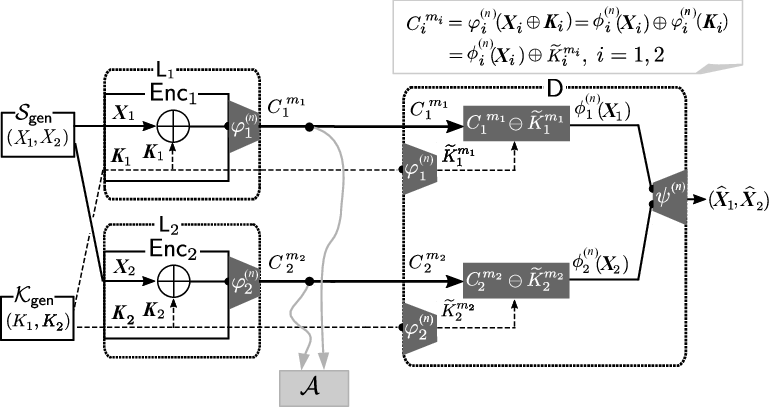
Fig. 3: Our proposed solution: linear encoders as privacy amplifiers.

In this section we outline the proof of Theorem 1. Our construction of (Φ1(n),Φ2(n),Ψ(n))(\Phi_{1}^{(n)},\Phi_{2}^{(n)},\Psi^{(n)}) is the same as that of Santoso and Oohama [1], [2] for the post encryption commpression scheme.

Let ϕ(n):=(ϕ1(n),ϕ2(n))\phi^{(n)}:=(\phi_{1}^{(n)},\phi_{2}^{(n)}) be a pair of linear mappings ϕ1(n):𝒳1n→𝒳1m1\phi_{1}^{(n)}:\mathcal{X}_{1}^{n}\rightarrow\mathcal{X}_{1}^{m_{1}} and ϕ2(n):𝒳2n→𝒳2m2\phi_{2}^{(n)}:\mathcal{X}_{2}^{n}\rightarrow\mathcal{X}_{2}^{m_{2}}. For each i=1,2i=1,2, we define the mapping ϕi(n)​𝒳in→𝒳imi\phi_{i}^{(n)}{\cal X}_{i}^{n}\to{\cal X}_{i}^{m_{i}} by

ϕi(n)​(𝒙i)=𝒙i​Ai​ for 𝐱i∈𝒳in,\phi_{i}^{(n)}({{\mbox{\boldmath$x$}}_{i}})={{\mbox{\boldmath$x$}}_{i}}A_{i}\mbox{ for }{{\mbox{\boldmath$x$}}_{i}}\in{\cal X}_{i}^{n}, (3)

where AiA_{i} is a matrix with nn rows and mim_{i} columns. For each i=1,2i=1,2, entries of AiA_{i} are from 𝒳i{\cal X}_{i}. We fix bimi∈𝒳imi,b_{i}^{m_{i}}\in\mathcal{X}_{i}^{m_{i}}, i=1,2i=1,2. For each i=1,2i=1,2, define the mapping φi(n):𝒳in→𝒳imi\varphi^{(n)}_{i}:{\cal X}_{i}^{n}\to{\cal X}_{i}^{m_{i}} by

φi(n)​(𝒌i):=ϕi(n)​(𝒌i)⊕bimi=𝒌i​Ai⊕bimi,\displaystyle\varphi_{i}^{(n)}({{\mbox{\boldmath$k$}}_{i}}):=\phi_{i}^{(n)}({{\mbox{\boldmath$k$}}_{i}})\oplus b_{i}^{m_{i}}={{\mbox{\boldmath$k$}}_{i}}A_{i}\oplus b_{i}^{m_{i}}, (4)

for 𝒌i∈𝒳in{{\mbox{\boldmath$k$}}_{i}}\in\mathcal{X}^{n}_{i}. For each i=1,2i=1,2, the mapping φi(n)\varphi_{i}^{(n)} is called the affine mapping induced by the linear mapping ϕi(n)\phi_{i}^{(n)} and constant vector bimib_{i}^{m_{i}} ∈𝒳mi\in{\cal X}^{m_{i}}. For each i=1,2i=1,2, define Φi(n)\Phi_{i}^{(n)} by

Φi(n)​(𝒌i,𝒙i)=φi(n)​(𝒌i⊕𝒙i).\Phi_{i}^{(n)}({\mbox{\boldmath$k$}}_{i},{\mbox{\boldmath$x$}}_{i})=\varphi_{i}^{(n)}({{\mbox{\boldmath$k$}}}_{i}\oplus{\mbox{\boldmath$x$}}_{i}).

By the definition (4) of φi(n)\varphi_{i}^{(n)}, i=1,2i=1,2, we have

Φi(n)​(𝒌i,𝒙i)=φi(n)​(𝒙i⊕𝒌i)\displaystyle\Phi_{i}^{(n)}({\mbox{\boldmath$k$}}_{i},{\mbox{\boldmath$x$}}_{i})=\varphi_{i}^{(n)}({{\mbox{\boldmath$x$}}_{i}}\oplus{{\mbox{\boldmath$k$}}_{i}})
=(𝒙i⊕𝒌i)​Ai⊕bimi=𝒙i​Ai⊕(𝒌i​Ai⊕bimi)\displaystyle=({{\mbox{\boldmath$x$}}_{i}}\oplus{{\mbox{\boldmath$k$}}_{i}})A_{i}\oplus b_{i}^{m_{i}}={{\mbox{\boldmath$x$}}_{i}}A_{i}\oplus({{\mbox{\boldmath$k$}}_{i}}A_{i}\oplus b_{i}^{m_{i}})
=ϕi(n)​(𝒙i)⊕φi(n)​(𝒌i), for 𝐱i,𝒌i∈𝒳in.\displaystyle=\phi_{i}^{(n)}({{\mbox{\boldmath$x$}}_{i}})\oplus\varphi_{i}^{(n)}({{\mbox{\boldmath$k$}}_{i}}),\mbox{ for }{{\mbox{\boldmath$x$}}_{i}},{{\mbox{\boldmath$k$}}_{i}}\in{\cal X}_{i}^{n}. (5)

Set φ(n):=(φ1(n),φ2(n))\varphi^{(n)}:=(\varphi_{1}^{(n)},\varphi_{2}^{(n)}). Next, let ψ(n)\psi^{(n)} be the corresponding joint decoder for ϕ(n)\phi^{(n)} such that ψ(n):𝒳1m1×𝒳2m2→𝒳1n×𝒳2n.\psi^{(n)}:\mathcal{X}_{1}^{m_{1}}\times\mathcal{X}_{2}^{m_{2}}\rightarrow\mathcal{X}_{1}^{n}\times\mathcal{X}_{2}^{n}. Note that ψ(n)\psi^{(n)} does not have a linear structure in general.

Description of Proposed procedure

We describe the procedure of our privacy amplified system as follows.

  1. 1.

    Encoding of Ciphertexts: First, we use φ1(n)\varphi_{1}^{(n)} and φ2(n)\varphi_{2}^{(n)} to encode the ciphertexts 𝑿1⊕𝑲1{\mbox{\boldmath$X$}}_{1}\oplus{\mbox{\boldmath$K$}}_{1} and 𝑿2⊕𝑲2{\mbox{\boldmath$X$}}_{2}\oplus{\mbox{\boldmath$K$}}_{2}. Let Cimi=φi(n)​(𝑿i⊕𝑲i)C_{i}^{m_{i}}=\varphi_{i}^{(n)}({\mbox{\boldmath$X$}}_{i}\oplus{{\mbox{\boldmath$K$}}}_{i}) for i=1,2i=1,2. By the affine structure (5) of encoders we have that for each i=1,2i=1,2,

    Φi(n)​(𝑲i,𝑿i)=Cimi=φi(n)​(𝑿i⊕𝑲i)\displaystyle\Phi_{i}^{(n)}({{\mbox{\boldmath$K$}}_{i}},{{\mbox{\boldmath$X$}}_{i}})={C}_{i}^{m_{i}}=\varphi_{i}^{(n)}({{\mbox{\boldmath$X$}}_{i}}\oplus{{\mbox{\boldmath$K$}}_{i}})
    =ϕi(n)​(𝑿i)⊕φi(n)​(𝑲i)=X~imi⊕K~imi,\displaystyle=\phi_{i}^{(n)}({{\mbox{\boldmath$X$}}_{i}})\oplus\varphi_{i}^{(n)}({{\mbox{\boldmath$K$}}_{i}})=\widetilde{X}_{i}^{m_{i}}\oplus\widetilde{K}_{i}^{m_{i}}, (6)

    where X~imi:=ϕi(n)​(𝑿i),K~imi:=φi(n)​(𝑲i).\widetilde{X}_{i}^{m_{i}}:=\phi_{i}^{(n)}({{\mbox{\boldmath$X$}}_{i}}),\widetilde{K}_{i}^{m_{i}}:=\varphi_{i}^{(n)}({{\mbox{\boldmath$K$}}_{i}}).

  2. 2.

    Decoding at Joint Sink Node 𝖣\mathsf{D}: First, using the pair of linear encoders (φ1(n),φ2(n))(\varphi_{1}^{(n)},\varphi_{2}^{(n)}), 𝖣\mathsf{D} encodes the keys (𝑲1,𝑲2)({{\mbox{\boldmath$K$}}_{1}},{{\mbox{\boldmath$K$}}_{2}}) which are received through private channel into (K~1m1,K~2m2)=(\widetilde{K}_{1}^{m_{1}},\widetilde{K}_{2}^{m_{2}})= (φ1(n)​(𝑲1),φ2(n)​(𝑲2))(\varphi_{1}^{(n)}({{\mbox{\boldmath$K$}}_{1}}),\varphi_{2}^{(n)}({{\mbox{\boldmath$K$}}_{2}})). Receiving (C1m1,C2m2)({C}_{1}^{m_{1}},{C}_{2}^{m_{2}}) from public communication channel, 𝖣\mathsf{D} computes X~imi,i=1,2\widetilde{X}_{i}^{m_{i}},i=1,2 in the following way. From (6), we have that for each i=1,2i=1,2, the decoder 𝖣\mathsf{D} can obtain X~imi=ϕi(n)​(𝑿i)\widetilde{X}_{i}^{m_{i}}=\phi_{i}^{(n)}({{\mbox{\boldmath$X$}}_{i}}) by subtracting K~imi=φi(n)​(𝑲i)\widetilde{K}_{i}^{m_{i}}=\varphi_{i}^{(n)}({{\mbox{\boldmath$K$}}_{i}}) from Cimi{C}_{i}^{m_{i}}. Finally, 𝖣\mathsf{D} outputs (𝑿^1,𝑿^2)(\widehat{\mbox{\boldmath$X$}}_{1},\widehat{\mbox{\boldmath$X$}}_{2}) by applying the joint decoder ψ(n)\psi^{(n)} to (X~1m1,X~2m2)(\widetilde{X}_{1}^{m_{1}},\widetilde{X}_{2}^{m_{2}}) as follows:

    (𝑿^1,𝑿^2)\displaystyle(\widehat{\mbox{\boldmath$X$}}_{1},\widehat{\mbox{\boldmath$X$}}_{2}) =(ψ(n)​(X~1m1,X~2m2))\displaystyle=(\psi^{(n)}(\widetilde{X}_{1}^{m_{1}},\widetilde{X}_{2}^{m_{2}}))
    =(ψ(n)​(ϕ1(n)​(𝑿1),ϕ2(n)​(𝑿2))CLOSE.\displaystyle=(\psi^{(n)}(\phi_{1}^{(n)}({{\mbox{\boldmath$X$}}_{1}}),\phi_{2}^{(n)}({{\mbox{\boldmath$X$}}_{2}})). (7)

    We summarize the above argument. For (𝑲1,𝑲2)({\mbox{\boldmath$K$}}_{1},{\mbox{\boldmath$K$}}_{2}) and (C1m1,C2m2)(C_{1}^{m_{1}},C_{2}^{m_{2}}), define Ψ(n)\Psi^{(n)} by

    Ψ(n)​(𝑲1,𝑲2,C1m1,C2m2)=Ψ𝑲1,𝑲2(n)​(C1m1,C2m2)\displaystyle\Psi^{(n)}({\mbox{\boldmath$K$}}_{1},{\mbox{\boldmath$K$}}_{2},C_{1}^{m_{1}},C_{2}^{m_{2}})=\Psi^{(n)}_{{\mbox{\scriptsize\boldmath$K$}}_{1},{\mbox{\scriptsize\boldmath$K$}}_{2}}(C_{1}^{m_{1}},C_{2}^{m_{2}})
    :=ψ(n)​(C1m1⊖K~1m1,C2m2⊖K~2m2)\displaystyle:=\psi^{(n)}({C}_{1}^{m_{1}}\ominus\widetilde{K}_{1}^{m_{1}},{C}_{2}^{m_{2}}\ominus\widetilde{K}_{2}^{m_{2}})
    =ψ(n)​(X~1m1,X~2m2).\displaystyle=\psi^{(n)}(\widetilde{X}_{1}^{m_{1}},\widetilde{X}_{2}^{m_{2}}).

    By the above definition and Cimi=Φi,𝑲i(n)(𝑿i),i=1,2,C_{i}^{m_{i}}=\Phi^{(n)}_{i,{{\mbox{\scriptsize\boldmath$K$}}}_{i}}({\mbox{\boldmath$X$}}_{i}),i=1,2, we have

    Ψ𝑲1,𝑲2(n)​(Φ1,𝑲1(n)​(𝑿1),Φ2,𝑲2(n)​(𝑿2))\displaystyle\Psi^{(n)}_{{\mbox{\scriptsize\boldmath$K$}}_{1},{\mbox{\scriptsize\boldmath$K$}}_{2}}(\Phi^{(n)}_{1,{\mbox{\scriptsize\boldmath$K$}}_{1}}({\mbox{\boldmath$X$}}_{1}),\Phi^{(n)}_{2,{\mbox{\scriptsize\boldmath$K$}}_{2}}({\mbox{\boldmath$X$}}_{2}))
    =ψ(n)​(X~1m1,X~2m2)=ψ(n)​(ϕ1(n)​(𝑿1),ϕ2(n)​(𝑿2)).\displaystyle=\psi^{(n)}(\widetilde{X}_{1}^{m_{1}},\widetilde{X}_{2}^{m_{2}})=\psi^{(n)}(\phi_{1}^{(n)}({\mbox{\boldmath$X$}}_{1}),\phi_{2}^{(n)}({\mbox{\boldmath$X$}}_{2})).

    Hence we have the condition which (Φ1(n),Φ2(n),Ψ(n))(\Phi^{(n)}_{1},\Phi^{(n)}_{2},\Psi^{(n)}) must satisfy.

In this paper, we use the minimum entropy decoder for our joint decoder ψ(n)\psi^{(n)}.
Minimum Entropy Decoder: For ϕi(n)(𝒙i)=x~imi,i=1,2\phi_{i}^{(n)}({\mbox{\boldmath$x$}}_{i})=\widetilde{x}_{i}^{m_{i}},i=1,2, ψ(n):𝒳1m1×𝒳2m2→𝒳1n×𝒳2n\psi^{(n)}:{\cal X}_{1}^{m_{1}}\times{\cal X}_{2}^{m_{2}}\to{\cal X}_{1}^{n}\times{\cal X}_{2}^{n} is defined as follows:

ψ(n)​(x~1m1,x~2m2)\displaystyle\psi^{(n)}(\widetilde{x}_{1}^{m_{1}},\widetilde{x}_{2}^{m_{2}})
:={(𝒙^1,𝒙^2)if ϕi(n)(𝒙^i)=x~imi,i=1,2,and ​H​(𝒙^1​𝒙^2)<H⁡(𝒙ˇ1​𝒙ˇ2)for all ​(𝒙ˇ1,𝒙ˇ2)​ such that ϕi(n)(𝒙ˇi)=x~imi,i=1,2,and ​(𝒙ˇ1,𝒙ˇ2)≠(𝒙^1,𝒙^2),arbitraryif there is no such ​(𝒙^1,𝒙^2)∈𝒳1n×𝒳2n.\displaystyle:=\left\{\begin{array}[]{cl}({\widehat{\mbox{\boldmath$x$}}_{1}},{\widehat{\mbox{\boldmath$x$}}_{2}})&\mbox{if }\phi_{i}^{(n)}({\widehat{\mbox{\boldmath$x$}}_{i}})=\widetilde{x}_{i}^{m_{i}},i=1,2,\\ &\mbox{and }H({\widehat{\mbox{\boldmath$x$}}_{1}}{\widehat{\mbox{\boldmath$x$}}_{2}})<H({\check{\mbox{\boldmath$x$}}_{1}}{\check{\mbox{\boldmath$x$}}_{2}})\\ &\mbox{for all }({\check{\mbox{\boldmath$x$}}_{1}},{\check{\mbox{\boldmath$x$}}_{2}})\mbox{ such that }\\ &\>\phi_{i}^{(n)}({\check{\mbox{\boldmath$x$}}_{i}})=\widetilde{x}_{i}^{m_{i}},i=1,2,\\ &\mbox{and }\>({\check{\mbox{\boldmath$x$}}_{1}},{\check{\mbox{\boldmath$x$}}_{2}})\neq({\widehat{\mbox{\boldmath$x$}}_{1}},{\widehat{\mbox{\boldmath$x$}}_{2}}),\\ \mbox{arbitrary}&\mbox{if there is no such }({\widehat{\mbox{\boldmath$x$}}_{1}},{\widehat{\mbox{\boldmath$x$}}_{2}})\in{\cal X}_{1}^{n}\times{\cal X}_{2}^{n}.\end{array}\right.

Our privacy amplified system described above is illustrated in Fig. 3.

Evaluations of the reliablility and security: On the error probability pep_{\rm e} of decoding we have

pe=Pr[Ψ(n)(𝑲1,𝑲2,ϕ1(n)(𝑲1,𝑿1),ϕ2(n)(𝑲2,𝑿2))\displaystyle p_{\rm e}=\Pr[\Psi^{(n)}({\mbox{\boldmath$K$}}_{1},{\mbox{\boldmath$K$}}_{2},\phi_{1}^{(n)}({{\mbox{\boldmath$K$}}_{1},{\mbox{\boldmath$X$}}_{1}}),\phi_{2}^{(n)}({{\mbox{\boldmath$K$}}_{2},{\mbox{\boldmath$X$}}_{2}}))
≠(𝑿1,𝑿2)]\displaystyle\qquad\neq({{\mbox{\boldmath$X$}}_{1}},{{\mbox{\boldmath$X$}}_{2}})]
=Pr[Ψ𝑲1,𝑲2(n)(Φ1,𝑲1(n)(𝑿1),Φ2,𝑲2(n)(𝑿2))≠(𝑿1,𝑿2)]\displaystyle=\Pr[\Psi^{(n)}_{{\mbox{\scriptsize\boldmath$K$}}_{1},{\mbox{\scriptsize\boldmath$K$}}_{2}}(\Phi_{1,{\mbox{\scriptsize\boldmath$K$}}_{1}}^{(n)}({\mbox{\boldmath$X$}}_{1}),\Phi_{2,{\mbox{\scriptsize\boldmath$K$}}_{2}}^{(n)}({\mbox{\boldmath$X$}}_{2}))\neq({{\mbox{\boldmath$X$}}_{1}},{{\mbox{\boldmath$X$}}_{2}})]
=Pr[ψ(n)(ϕ1(n)(𝑿1),ϕ2(n)(𝑿2))≠(𝑿1,𝑿2)].\displaystyle=\Pr[\psi^{(n)}(\phi_{1}^{(n)}({\mbox{\boldmath$X$}}_{1}),\phi_{2}^{(n)}({\mbox{\boldmath$X$}}_{2}))\neq({\mbox{\boldmath$X$}}_{1},{\mbox{\boldmath$X$}}_{2})].

We have the following upper bound of Δmax−MI(n)​(Φ1(n),Φ2(n)CLOSE,\Delta_{{\rm max-MI}}^{(n)}(\Phi_{1}^{(n)},\Phi_{2}^{(n)}, OPENΨ(n)|pK1​K2n)\Psi^{(n)}|{p}_{K_{1}K_{2}}^{n}).

Lemma 2

For the proposed construction of (Φ1(n),Φ2(n)𝐶𝐿𝑂𝑆𝐸,(\Phi^{(n)}_{1},\Phi^{(n)}_{2}, 𝑂𝑃𝐸𝑁Ψ(n))\Psi^{(n)}), we have

Δmax−MI(n)​(Φ1(n),Φ2(n),Ψ(n)|pK1​K2n)\displaystyle\Delta_{{\rm max-MI}}^{(n)}(\Phi_{1}^{(n)},\Phi_{2}^{(n)},\Psi^{(n)}|{p}_{K_{1}K_{2}}^{n})
≤Δ¯max−MI(n)​(Φ1(n),Φ2(n)|pK1​K2n)\displaystyle\leq\overline{\Delta}_{{\rm max-MI}}^{(n)}(\Phi_{1}^{(n)},\Phi_{2}^{(n)}|{p}_{K_{1}K_{2}}^{n})
≤m1​log⁡|𝒳1|+m2​log|𝒳2|−H⁡(K~1m1​K~2m2)\displaystyle\leq m_{1}\log|{\cal X}_{1}|+m_{2}\log|{\cal X}_{2}|-H(\widetilde{K}_{1}^{m_{1}}\widetilde{K}_{2}^{m_{2}})
=D(pK~1m1​K~2m2∥pU1m1​U2m2).\displaystyle=D(p_{\widetilde{K}_{1}^{m_{1}}\widetilde{K}_{2}^{m_{2}}}\|p_{{U}_{1}^{m_{1}}{U}_{2}^{m_{2}}}).

Here pU1m1​U2m2p_{{U}_{1}^{m_{1}}{U}_{2}^{m_{2}}} is the uniform distribution over 𝒳1m1×𝒳2m2{\cal X}_{1}^{m_{1}}\times{\cal X}_{2}^{m_{2}}.

Proof:

By Proposition 1 part a), it sufficies to prove the upper bound of Δ¯max−MI(n)​(Φ1(n),Φ2(n)|pK1​K2n).\overline{\Delta}_{{\rm max-MI}}^{(n)}(\Phi_{1}^{(n)},\Phi_{2}^{(n)}|{p}_{K_{1}K_{2}}^{n}). For the proposed construction of (Φ1(n),Φ2(n))(\Phi_{1}^{(n)},\Phi_{2}^{(n)}), we have

C¯imi=K~imi⊕ϕi(n)(𝑿¯i),i=1,2.\displaystyle\overline{C}_{i}^{m_{i}}=\widetilde{K}_{i}^{m_{i}}\oplus\phi_{i}^{(n)}(\overline{{\mbox{\boldmath$X$}}}_{i}),i=1,2. (8)

Then we have the following chain of inequalities:

I⁡(C¯1m1​C¯1m1,𝑿¯1​𝑿¯2)\displaystyle I(\overline{C}_{1}^{m_{1}}\overline{C}_{1}^{m_{1}};\overline{{\mbox{\boldmath$X$}}}_{1}\overline{{\mbox{\boldmath$X$}}}_{2})
=H⁡(C¯1m1​C¯2m2)−H⁡(C¯1m1​C¯2m2|𝑿¯1​𝑿¯2)\displaystyle=H(\overline{C}_{1}^{m_{1}}\overline{C}_{2}^{m_{2}})-H(\overline{C}_{1}^{m_{1}}\overline{C}_{2}^{m_{2}}|\overline{{\mbox{\boldmath$X$}}}_{1}\overline{{\mbox{\boldmath$X$}}}_{2})
≤m1​log⁡|𝒳1|+m2​log|𝒳2|−H⁡(C¯1m1​C¯2m2|𝑿¯1​𝑿¯2)\displaystyle\leq m_{1}\log|{\cal X}_{1}|+m_{2}\log|{\cal X}_{2}|-H(\overline{C}_{1}^{m_{1}}\overline{C}_{2}^{m_{2}}|\overline{{\mbox{\boldmath$X$}}}_{1}\overline{{\mbox{\boldmath$X$}}}_{2})
=(a)m1​log⁡|𝒳1|+m2​log⁡|𝒳2|\displaystyle\stackrel{{\scriptstyle{\rm(a)}}}{{=}}m_{1}\log|{\cal X}_{1}|+m_{2}\log|{\cal X}_{2}|
−H⁡(K~1m1⊕ϕ1(n)​(𝑿¯1),K~2m2⊕ϕ2(n)​(𝑿¯2)|𝑿¯1​𝑿¯2)\displaystyle\quad-H(\widetilde{K}_{1}^{m_{1}}\oplus\phi_{1}^{(n)}(\overline{{\mbox{\boldmath$X$}}}_{1}),\widetilde{K}_{2}^{m_{2}}\oplus\phi_{2}^{(n)}(\overline{{\mbox{\boldmath$X$}}}_{2})|\overline{{\mbox{\boldmath$X$}}}_{1}\overline{{\mbox{\boldmath$X$}}}_{2})
=m1​log⁡|𝒳1|+m2​log|𝒳2|−H⁡(K~1m1​K~2m2|𝑿¯1​𝑿¯2)\displaystyle=m_{1}\log|{\cal X}_{1}|+m_{2}\log|{\cal X}_{2}|-H(\widetilde{K}_{1}^{m_{1}}\widetilde{K}_{2}^{m_{2}}|\overline{{\mbox{\boldmath$X$}}}_{1}\overline{{\mbox{\boldmath$X$}}}_{2})
=(b)m1​log⁡|𝒳1|+m2​log|𝒳2|−H⁡(K~1m1​K~2m2)\displaystyle\stackrel{{\scriptstyle{\rm(b)}}}{{=}}m_{1}\log|{\cal X}_{1}|+m_{2}\log|{\cal X}_{2}|-H(\widetilde{K}_{1}^{m_{1}}\widetilde{K}_{2}^{m_{2}})
=D(pK~1m1​K~2m2∥pU1m1​U2m2).\displaystyle=D(p_{\widetilde{K}_{1}^{m_{1}}\widetilde{K}_{2}^{m_{2}}}\|p_{{U}_{1}^{m_{1}}{U}_{2}^{m_{2}}}). (9)

Step (a) follows from (8). Step (b) follows from (𝐗¯1,𝐗¯2)(\overline{{\mbox{\boldmath$X$}}}_{1},\overline{{\mbox{\boldmath$X$}}}_{2}) ⟂(𝐊1,𝐊2)\perp({\mbox{\boldmath$K$}}_{1},{\mbox{\boldmath$K$}}_{2}). Since (9) holds for any (𝐗¯1,𝐗¯2)(\overline{{\mbox{\boldmath$X$}}}_{1},\overline{{\mbox{\boldmath$X$}}}_{2}), we have the upper bound of Δ¯max−MI(n)​(Φ1(n),Φ2(n)|pK1​K2n)\overline{\Delta}_{{\rm max-MI}}^{(n)}(\Phi_{1}^{(n)},\Phi_{2}^{(n)}|{p}_{K_{1}K_{2}}^{n}) in Lemma 2. ∎According to Santoso and Oohama [2], ∃{(Φ1(n),Φ2(n),\exists\{(\Phi_{1}^{(n)},\Phi_{2}^{(n)}, Ψ(n))}n≥1\Psi^{(n)})\}_{n\geq 1} such that for any (pX1​X2,pK1​K2)(p_{X_{1}X_{2}},p_{K_{1}K_{2}}) satisfying

(m1n​log⁡|𝒳1|,m2n​log⁡|𝒳2|)\displaystyle\left(\frac{m_{1}}{n}\log|{\cal X}_{1}|,\frac{m_{2}}{n}\log|{\cal X}_{2}|\right)
∈ℛkey​(pK1​K2)∩ℛsw​(pX1​X2),\displaystyle\in\mathcal{R}_{\mathrm{key}}(p_{K_{1}K_{2}})\cap\mathcal{R}_{\mathrm{sw}}(p_{X_{1}X_{2}}),

the two quantities

Pr[ψ(n)(ϕ1(n)(𝑿1),ϕ2(n)(𝑿2))≠(𝑿1,𝑿2)] and\displaystyle\Pr[\psi^{(n)}(\phi_{1}^{(n)}({\mbox{\boldmath$X$}}_{1}),\phi_{2}^{(n)}({\mbox{\boldmath$X$}}_{2}))\neq({\mbox{\boldmath$X$}}_{1},{\mbox{\boldmath$X$}}_{2})]\mbox{ and }
D(pK~1m1​K~2m2∥pU1m1​U2m2)\displaystyle D(p_{\widetilde{K}_{1}^{m_{1}}\widetilde{K}_{2}^{m_{2}}}\|p_{{U}_{1}^{m_{1}}{U}_{2}^{m_{2}}})

decay exponentially as nn tends to infinity. Hence we have Theorem 1.

-A Proof of Property 1

Proof:

We have the following:

𝒟(n)=(a)\displaystyle{\cal D}^{(n)}\stackrel{{\scriptstyle{\rm(a)}}}{{=}} {(𝒙1,𝒙2)=ψ(n)(x~1m1,x~2m2):\displaystyle\{({\mbox{\boldmath$x$}}_{1},{\mbox{\boldmath$x$}}_{2})=\psi^{(n)}(\tilde{x}_{1}^{m_{1}},\tilde{x}_{2}^{m_{2}}):
(x~1m1,x~2m2)∈ϕ1(n)(𝒳1n)×ϕ2(n)(𝒳2n)}\displaystyle\quad(\tilde{x}_{1}^{m_{1}},\tilde{x}_{2}^{m_{2}})\in\phi_{1}^{(n)}({\cal X}_{1}^{n})\times\phi_{2}^{(n)}({\cal X}_{2}^{n})\}
=(b)\displaystyle\stackrel{{\scriptstyle{\rm(b)}}}{{=}} {(𝒙1,𝒙2)=ψ(n)(x~1m1,x~2m2):\displaystyle\{({\mbox{\boldmath$x$}}_{1},{\mbox{\boldmath$x$}}_{2})=\psi^{(n)}(\tilde{x}_{1}^{m_{1}},\tilde{x}_{2}^{m_{2}}):
(x~1m1,x~2m2)∈𝒳1m1×𝒳2m2}.\displaystyle\quad(\tilde{x}_{1}^{m_{1}},\tilde{x}_{2}^{m_{2}})\in{\cal X}_{1}^{m_{1}}\times{\cal X}_{2}^{m_{2}}\}. (10)

Step (a) follows from that every pair (x~1m1,x~2m2)∈ϕ1(n)(𝒳1n)×ϕ2(n)(𝒳2n)}(\tilde{x}_{1}^{m_{1}},\tilde{x}_{2}^{m_{2}})\in\phi_{1}^{(n)}({\cal X}_{1}^{n})\times\phi_{2}^{(n)}({\cal X}_{2}^{n})\} uniquely determines (𝐱1,𝐱2)∈𝒟(n)({\mbox{\boldmath$x$}}_{1},{\mbox{\boldmath$x$}}_{2})\in{\cal D}^{(n)}. Step (b) follows from that ϕi(n),i=1,2\phi_{i}^{(n)},i=1,2 are surjective. Since ψ(n):𝒳1m1×𝒳2m2→𝒳1n×𝒳2n\psi^{(n)}:{\cal X}_{1}^{m_{1}}\times{\cal X}_{2}^{m_{2}}\to{\cal X}_{1}^{n}\times{\cal X}_{2}^{n} is a one-to-one mapping and (10), we have |𝒟(n)|=|𝒳1m1|​|𝒳2m2|.|{\cal D}^{(n)}|=|{\cal X}_{1}^{m_{1}}||{\cal X}_{2}^{m_{2}}|. ∎

-B Proof of Property 2

We frist prove the part a) and next prove the part b).

Proof:

Under (𝐱1,𝐱2),(𝐱1′,𝐱2′)∈𝒟(n)({\mbox{\boldmath$x$}}_{1},{\mbox{\boldmath$x$}}_{2}),({\mbox{\boldmath$x$}}_{1}^{\prime},{\mbox{\boldmath$x$}}_{2}^{\prime})\in{\cal D}^{(n)} and (𝐱1,𝐱2)≠({\mbox{\boldmath$x$}}_{1},{\mbox{\boldmath$x$}}_{2})\neq (𝐱1′,𝐱2′)({\mbox{\boldmath$x$}}_{1}^{\prime},{\mbox{\boldmath$x$}}_{2}^{\prime}), we assume that

(Φ1,𝒌1(n)​(𝒙1),Φ2,𝒌2(n)​(𝒙2))=(Φ1,𝒌1(n)​(𝒙1′),Φ2,𝒌2(n)​(𝒙2′)).(\Phi^{(n)}_{1,{\mbox{\scriptsize\boldmath$k$}}_{1}}({{\mbox{\boldmath$x$}}_{1}}),\Phi^{(n)}_{2,{\mbox{\scriptsize\boldmath$k$}}_{2}}({{\mbox{\boldmath$x$}}_{2}}))=(\Phi^{(n)}_{1,{\mbox{\scriptsize\boldmath$k$}}_{1}}({{\mbox{\boldmath$x$}}}_{1}^{\prime}),\Phi^{(n)}_{2,{\mbox{\scriptsize\boldmath$k$}}_{2}}({{\mbox{\boldmath$x$}}}_{2}^{\prime})). (11)

Then we have the following

(𝒙1,𝒙2)=(a)ψ(n)​(ϕ1(n)​(𝒌1),ϕ2(n)​(𝒌2)CLOSE,\displaystyle({\mbox{\boldmath$x$}}_{1},{\mbox{\boldmath$x$}}_{2})\stackrel{{\scriptstyle{\rm(a)}}}{{=}}\psi^{(n)}(\phi_{1}^{(n)}({\mbox{\boldmath$k$}}_{1}),\phi_{2}^{(n)}({\mbox{\boldmath$k$}}_{2}),
=(b)Ψ𝒌1,𝒌2(n)​(Φ1,𝒌1(n)​(𝒙1),Φ2,𝒌2(n)​(𝒙2))\displaystyle\stackrel{{\scriptstyle{\rm(b)}}}{{=}}\Psi^{(n)}_{{\mbox{\scriptsize\boldmath$k$}}_{1},{\mbox{\scriptsize\boldmath$k$}}_{2}}(\Phi^{(n)}_{1,{\mbox{\scriptsize\boldmath$k$}}_{1}}({{\mbox{\boldmath$x$}}_{1}}),\Phi^{(n)}_{2,{\mbox{\scriptsize\boldmath$k$}}_{2}}({{\mbox{\boldmath$x$}}_{2}}))
=(c)Ψ𝒌1,𝒌2(n)​(Φ1,𝒌1(n)​(𝒙1′),Φ2,𝒌2(n)​(𝒙2′))\displaystyle\stackrel{{\scriptstyle{\rm(c)}}}{{=}}\Psi^{(n)}_{{\mbox{\scriptsize\boldmath$k$}}_{1},{\mbox{\scriptsize\boldmath$k$}}_{2}}(\Phi^{(n)}_{1,{\mbox{\scriptsize\boldmath$k$}}_{1}}({{\mbox{\boldmath$x$}}}_{1}^{\prime}),\Phi^{(n)}_{2,{\mbox{\scriptsize\boldmath$k$}}_{2}}({{\mbox{\boldmath$x$}}}_{2}^{\prime}))
=(d)ψ(n)​(ϕ1(n)​(𝒙1′),ϕ2(n)​(𝒙2′))=(e)(𝒙1′,𝒙2′).\displaystyle\stackrel{{\scriptstyle{\rm(d)}}}{{=}}\psi^{(n)}(\phi^{(n)}_{1}({{\mbox{\boldmath$x$}}}_{1}^{\prime}),\phi^{(n)}_{2}({{\mbox{\boldmath$x$}}}_{2}^{\prime}))\stackrel{{\scriptstyle{\rm(e)}}}{{=}}({{\mbox{\boldmath$x$}}}_{1}^{\prime},{{\mbox{\boldmath$x$}}}_{2}^{\prime}). (12)

Steps (a) and (e) follow from the definition of 𝒟(n){\cal D}^{(n)}. Step (c) follows from 11. Steps (b) and (d) follow from the relationship between (ϕ1(n),ϕ2(n),ψ(n))(\phi^{(n)}_{1},\phi^{(n)}_{2},\psi^{(n)}) and (Φ1,𝐤1(n),Φ2,𝐤2(n),Ψ𝐤1,𝐤2(n)).(\Phi^{(n)}_{1,{\mbox{\scriptsize\boldmath$k$}}_{1}},\Phi^{(n)}_{2,{\mbox{\scriptsize\boldmath$k$}}_{2}},\Psi^{(n)}_{{\mbox{\scriptsize\boldmath$k$}}_{1},{\mbox{\scriptsize\boldmath$k$}}_{2}}). The equality (12) contradics the first assumption. Hence we must have Property 2 part a). ∎

Proof:

We assume that ∃(𝐤1,𝐤2)\exists({\mbox{\boldmath$k$}}_{1},{\mbox{\boldmath$k$}}_{2}) and ∃(c1m1,c2m2)\exists(c_{1}^{m_{1}},c_{2}^{m_{2}}) such that ∀(𝐱1,𝐱2)∈𝒟(n)\forall({\mbox{\boldmath$x$}}_{1},{\mbox{\boldmath$x$}}_{2})\in{\cal D}^{(n)}, (Φ1,𝐤1(n)​(𝐱1)𝐶𝐿𝑂𝑆𝐸,(\Phi^{(n)}_{1,{\mbox{\scriptsize\boldmath$k$}}_{1}}({\mbox{\boldmath$x$}}_{1}), 𝑂𝑃𝐸𝑁Φ2,𝐤2(n)​(𝐱2))\Phi^{(n)}_{2,{\mbox{\scriptsize\boldmath$k$}}_{2}}({\mbox{\boldmath$x$}}_{2})) ≠\neq (c1m1,c2m2)(c_{1}^{m_{1}},c_{2}^{m_{2}}). Set B :={ (Φ^(n)_1,𝐤k_1(𝐱x_1), Φ^(n)_2,𝐱x_2(𝐱x_2)): (𝐱x_1,𝐱x_2)∈D^(n) }. Then by the above assumption we have

ℬ⊆𝒳1m1×𝒳2m2−{(c1m1,c2m2)}.\displaystyle{\cal B}\subseteq{\cal X}_{1}^{m_{1}}\times{\cal X}_{2}^{m_{2}}-\left\{(c_{1}^{m_{1}},c_{2}^{m_{2}})\right\}. (13)

On the other hand we have

Ψ𝒌1,𝒌2(n)​(ℬ)\displaystyle\Psi^{(n)}_{{\mbox{\scriptsize\boldmath$k$}}_{1},{\mbox{\scriptsize\boldmath$k$}}_{2}}({\cal B})
={Ψ𝒌1,𝒌2(n)​(Φ1,𝒌1(n)​(𝒙1),Φ2,𝒌2(n)​(𝒙2)):(𝒙1,𝒙2)∈𝒟(n)}\displaystyle=\left\{\Psi^{(n)}_{{\mbox{\scriptsize\boldmath$k$}}_{1},{\mbox{\scriptsize\boldmath$k$}}_{2}}(\Phi^{(n)}_{1,{\mbox{\scriptsize\boldmath$k$}}_{1}}({\mbox{\boldmath$x$}}_{1}),\Phi^{(n)}_{2,{\mbox{\scriptsize\boldmath$k$}}_{2}}({\mbox{\boldmath$x$}}_{2})):({\mbox{\boldmath$x$}}_{1},{\mbox{\boldmath$x$}}_{2})\in{\cal D}^{(n)}\right\}
={ψ(n)​(ϕ1(n)​(𝒙1),ϕ2(n)​(𝒙2)):(𝒙1,𝒙2)∈𝒟(n)}=𝒟(n),\displaystyle=\left\{\psi^{(n)}(\phi^{(n)}_{1}({\mbox{\boldmath$x$}}_{1}),\phi^{(n)}_{2}({\mbox{\boldmath$x$}}_{2})):({\mbox{\boldmath$x$}}_{1},{\mbox{\boldmath$x$}}_{2})\in{\cal D}^{(n)}\right\}={\cal D}^{(n)},

which together with that Ψ𝐤1,𝐤2(n):\Psi_{{\mbox{\scriptsize\boldmath$k$}}_{1},{\mbox{\scriptsize\boldmath$k$}}_{2}}^{(n)}: 𝒳1m1×𝒳2m2{\cal X}_{1}^{m_{1}}\times{\cal X}_{2}^{m_{2}}→\to 𝒳1n×𝒳2n{\cal X}_{1}^{n}\times{\cal X}_{2}^{n} is a one-to-one mapping yields that

|ℬ|=|Ψ𝒌1,𝒌2(n)​(ℬ)|=|𝒟(n)|=|𝒳1m1|​|𝒳2m2|.\displaystyle|{\cal B}|=|\Psi^{(n)}_{{\mbox{\scriptsize\boldmath$k$}}_{1},{\mbox{\scriptsize\boldmath$k$}}_{2}}({\cal B})|=|{\cal D}^{(n)}|=|{\cal X}_{1}^{m_{1}}||{\cal X}_{2}^{m_{2}}|.

The above equality contradicts (13). Hence we must have that ∀(𝐤1,𝐤2),\forall({\mbox{\boldmath$k$}}_{1},{\mbox{\boldmath$k$}}_{2}), ∀(c1m1,c2m2),\forall(c_{1}^{m_{1}},c_{2}^{m_{2}}), ∃(𝐱1,𝐱2)∈𝒟(n)\exists({\mbox{\boldmath$x$}}_{1},{\mbox{\boldmath$x$}}_{2})\in{\cal D}^{(n)} such that Φi,𝐤i(n)(𝐱i)=cimi,i=1,2\Phi^{(n)}_{i,{{\mbox{\scriptsize\boldmath$k$}}}_{i}}({\mbox{\boldmath$x$}}_{i})=c_{i}^{m_{i}},i=1,2. ∎

-C Proof of Lemma 1

In this appendix we prove Lemma 1.

Proof:

By definition we have

pC1m1​C2m2|𝑿1​𝑿2(c1m1,c2m2|𝒙1,𝒙2)\displaystyle p_{C_{1}^{m_{1}}C_{2}^{m_{2}}|{\mbox{\scriptsize\boldmath$X$}}_{1}{\mbox{\scriptsize\boldmath$X$}}_{2}}(c_{1}^{m_{1}},c_{2}^{m_{2}}|{\mbox{\boldmath$x$}}_{1},{\mbox{\boldmath$x$}}_{2})
=Pr{(𝑲1,𝑲2)∈𝒜𝒙1,𝒙2(c1m1,c2m2)|𝑿1=𝒙1,𝑿2=𝒙2}\displaystyle={\rm Pr}\left\{({\mbox{\boldmath$K$}}_{1},{\mbox{\boldmath$K$}}_{2})\in{\cal A}_{{\mbox{\scriptsize\boldmath$x$}}_{1},{\mbox{\scriptsize\boldmath$x$}}_{2}}(c_{1}^{m_{1}},c_{2}^{m_{2}})\Bigl|{\mbox{\boldmath$X$}}_{1}={\mbox{\boldmath$x$}}_{1},{\mbox{\boldmath$X$}}_{2}={\mbox{\boldmath$x$}}_{2}\right\}
=(a)Pr{(𝑲1,𝑲2)∈𝒜𝒙1,𝒙2(c1m1,c2m2)}.\displaystyle\stackrel{{\scriptstyle{\rm(a)}}}{{=}}{\rm Pr}\left\{({\mbox{\boldmath$K$}}_{1},{\mbox{\boldmath$K$}}_{2})\in{\cal A}_{{\mbox{\scriptsize\boldmath$x$}}_{1},{\mbox{\scriptsize\boldmath$x$}}_{2}}(c_{1}^{m_{1}},c_{2}^{m_{2}})\right\}. (14)

Step (a) follows from (𝐊1,𝐊2)⟂(𝐗1,𝐗2)({\mbox{\boldmath$K$}}_{1},{\mbox{\boldmath$K$}}_{2})\perp({\mbox{\boldmath$X$}}_{1},{\mbox{\boldmath$X$}}_{2}). On the other hand, Property 2 part a) implies that

𝒜𝒙1,𝒙2​(c1m1,c2m2)∩𝒜𝒙1′,𝒙2′​(c1m1,c2m2)=∅\displaystyle{\cal A}_{{\mbox{\scriptsize\boldmath$x$}}_{1},{\mbox{\scriptsize\boldmath$x$}}_{2}}(c_{1}^{m_{1}},c_{2}^{m_{2}})\cap{\cal A}_{{{\mbox{\scriptsize\boldmath$x$}}}^{\prime}_{1},{{\mbox{\scriptsize\boldmath$x$}}}^{\prime}_{2}}(c_{1}^{m_{1}},c_{2}^{m_{2}})=\emptyset
for ​(𝒙1,𝒙2)≠(𝒙1′,𝒙2′)∈𝒟(n).\displaystyle\mbox{ for }({\mbox{\boldmath$x$}}_{1},{\mbox{\boldmath$x$}}_{2})\neq({{\mbox{\boldmath$x$}}}^{\prime}_{1},{{\mbox{\boldmath$x$}}}^{\prime}_{2})\in{\cal D}^{(n)}. (15)

Furthermore, Property 2 part b) implies that

⋃(𝒙1,𝒙2)∈𝒟(n)𝒜𝒙1,𝒙2​(c1m1,c2m2)=𝒳1n×𝒳2n.\displaystyle\bigcup_{({\mbox{\scriptsize\boldmath$x$}}_{1},{\mbox{\scriptsize\boldmath$x$}}_{2})\in{\cal D}^{(n)}}{\cal A}_{{\mbox{\scriptsize\boldmath$x$}}_{1},{\mbox{\scriptsize\boldmath$x$}}_{2}}(c_{1}^{m_{1}},c_{2}^{m_{2}})={\cal X}_{1}^{n}\times{\cal X}_{2}^{n}. (16)

From (14), we have the following chain of equalities:

∑(𝒙1,𝒙2)∈𝒟(n)pC1m1​C2m2|𝑿1​𝑿2(c1m1,c2m2|𝒙1,𝒙2)\displaystyle\sum_{({\mbox{\scriptsize\boldmath$x$}}_{1},{\mbox{\scriptsize\boldmath$x$}}_{2})\in{\cal D}^{(n)}}p_{C_{1}^{m_{1}}C_{2}^{m_{2}}|{\mbox{\scriptsize\boldmath$X$}}_{1}{\mbox{\scriptsize\boldmath$X$}}_{2}}(c_{1}^{m_{1}},c_{2}^{m_{2}}|{\mbox{\boldmath$x$}}_{1},{\mbox{\boldmath$x$}}_{2})
=(a)Pr{(𝑲1,𝑲2)∈⋃(𝒙1,𝒙2)∈𝒟(n)𝒜𝒙1,𝒙2(c1m1,c2m2)}=(b)1.\displaystyle\stackrel{{\scriptstyle{\rm(a)}}}{{=}}\Pr\left\{({\mbox{\boldmath$K$}}_{1},{\mbox{\boldmath$K$}}_{2})\in\bigcup_{({\mbox{\scriptsize\boldmath$x$}}_{1},{\mbox{\scriptsize\boldmath$x$}}_{2})\in{\cal D}^{(n)}}{\cal A}_{{\mbox{\scriptsize\boldmath$x$}}_{1},{\mbox{\scriptsize\boldmath$x$}}_{2}}(c_{1}^{m_{1}},c_{2}^{m_{2}})\right\}\stackrel{{\scriptstyle{\rm(b)}}}{{=}}1.

Step (a) follows from (15). Step (b) follows from (16). ∎

-D Proof of Proposition 1

In this appendix we prove Proposition 1.

Proof:

The part a) is obvious. We first prove the part b). Using the quntities

Γ𝑲1​𝑲2,(𝒙1,𝒙2)​(c1m1,c2m2),\displaystyle\Gamma_{{\mbox{\scriptsize\boldmath$K$}}_{1}{\mbox{\scriptsize\boldmath$K$}}_{2},({\mbox{\scriptsize\boldmath$x$}}_{1},{\mbox{\scriptsize\boldmath$x$}}_{2})}(c_{1}^{m_{1}},c_{2}^{m_{2}}),
(𝒙1,𝒙2,c1m1,c1m1)∈𝒳1n×𝒳2n×𝒳m1×𝒳m1,\displaystyle({\mbox{\boldmath$x$}}_{1},{\mbox{\boldmath$x$}}_{2},c_{1}^{m_{1}},c_{1}^{m_{1}})\in{\cal X}_{1}^{n}\times{\cal X}_{2}^{n}\times{\cal X}^{m_{1}}\times{\cal X}^{m_{1}},

components pC1m1​C2m2|𝐗1​𝐗2​(c1m1,c2m2)p_{C_{1}^{m_{1}}C_{2}^{m_{2}}|{\mbox{\scriptsize\boldmath$X$}}_{1}{\mbox{\scriptsize\boldmath$X$}}_{2}}(c_{1}^{m_{1}},c_{2}^{m_{2}}) of the joint distribution pC1m1​C2m2p_{C_{1}^{m_{1}}C_{2}^{m_{2}}} can be computed as

pC1m1​C2m2​(c1m1,c2m2)\displaystyle p_{C_{1}^{m_{1}}C_{2}^{m_{2}}}(c_{1}^{m_{1}},c_{2}^{m_{2}})
=∑(𝒙1,𝒙2)p𝑿1​𝑿2​(𝒙1,𝒙2)​Γ𝑲1​𝑲2,(𝒙1,𝒙2)​(c1m1​c2m2).\displaystyle=\sum_{({\mbox{\scriptsize\boldmath$x$}}_{1},{\mbox{\scriptsize\boldmath$x$}}_{2})}p_{{\mbox{\scriptsize\boldmath$X$}}_{1}{\mbox{\scriptsize\boldmath$X$}}_{2}}({\mbox{\boldmath$x$}}_{1},{\mbox{\boldmath$x$}}_{2})\Gamma_{{\mbox{\scriptsize\boldmath$K$}}_{1}{\mbox{\scriptsize\boldmath$K$}}_{2},({\mbox{\scriptsize\boldmath$x$}}_{1},{\mbox{\scriptsize\boldmath$x$}}_{2})}(c_{1}^{m_{1}}c_{2}^{m_{2}}).

Set

Γ𝑲1​𝑲2(p𝑿1​𝑿2)​(c1m1,c2m2)\displaystyle\Gamma_{{\mbox{\scriptsize\boldmath$K$}}_{1}{\mbox{\scriptsize\boldmath$K$}}_{2}}^{(p_{{\mbox{\tiny\boldmath$X$}}_{1}{\mbox{\tiny\boldmath$X$}}_{2}})}(c_{1}^{m_{1}},c_{2}^{m_{2}})
=∑(𝒙1,𝒙2)p𝑿1​𝑿2​(𝒙1,𝒙2)​Γ𝑲1​𝑲2,(𝒙1,𝒙2)​(c1m1,c2m2)\displaystyle=\sum_{({\mbox{\scriptsize\boldmath$x$}}_{1},{\mbox{\scriptsize\boldmath$x$}}_{2})}p_{{\mbox{\scriptsize\boldmath$X$}}_{1}{\mbox{\scriptsize\boldmath$X$}}_{2}}({\mbox{\boldmath$x$}}_{1},{\mbox{\boldmath$x$}}_{2})\Gamma_{{\mbox{\scriptsize\boldmath$K$}}_{1}{\mbox{\scriptsize\boldmath$K$}}_{2},({\mbox{\scriptsize\boldmath$x$}}_{1},{\mbox{\scriptsize\boldmath$x$}}_{2})}(c_{1}^{m_{1}},c_{2}^{m_{2}})
=pC1m1​C2m2​(c1m1,c2m2).\displaystyle=p_{C_{1}^{m_{1}}C_{2}^{m_{2}}}(c_{1}^{m_{1}},c_{2}^{m_{2}}).

Furthermore, set

Γ𝑲1​𝑲2(p𝑿1​𝑿2):={Γ𝑲1​𝑲2(p𝑿1​𝑿2)​(c1m1,c2m2)}(c1m1,c2m2)∈𝒳1m1×𝒳2m2\displaystyle\Gamma^{(p_{{\mbox{\tiny\boldmath$X$}}_{1}{\mbox{\tiny\boldmath$X$}}_{2}})}_{{\mbox{\scriptsize\boldmath$K$}}_{1}{\mbox{\scriptsize\boldmath$K$}}_{2}}:=\left\{\Gamma_{{\mbox{\scriptsize\boldmath$K$}}_{1}{\mbox{\scriptsize\boldmath$K$}}_{2}}^{(p_{{\mbox{\tiny\boldmath$X$}}_{1}{\mbox{\tiny\boldmath$X$}}_{2}})}(c_{1}^{m_{1}},c_{2}^{m_{2}})\right\}_{(c_{1}^{m_{1}},c_{2}^{m_{2}})\in{\cal X}_{1}^{m_{1}}\times{\cal X}_{2}^{m_{2}}}
=pC1m1​C2m2.\displaystyle=p_{C_{1}^{m_{1}}C_{2}^{m_{2}}}.

Using Γ𝐊1​𝐊1,(𝐱1,𝐱2),(𝐱1,𝐱2)∈𝒳1n×𝒳2n\Gamma_{{\mbox{\scriptsize\boldmath$K$}}_{1}{\mbox{\scriptsize\boldmath$K$}}_{1},({\mbox{\scriptsize\boldmath$x$}}_{1},{\mbox{\scriptsize\boldmath$x$}}_{2})},({\mbox{\boldmath$x$}}_{1},{\mbox{\boldmath$x$}}_{2})\in{\cal X}_{1}^{n}\times{\cal X}_{2}^{n} and Γ𝐊1​𝐊2(p𝐗1​𝐗2)\Gamma_{{\mbox{\scriptsize\boldmath$K$}}_{1}{\mbox{\scriptsize\boldmath$K$}}_{2}}^{(p_{{\mbox{\tiny\boldmath$X$}}_{1}{\mbox{\tiny\boldmath$X$}}_{2}})}, we compute ΔMI(n)\Delta_{\rm MI}^{(n)} to obtain

ΔMI(n)=I⁡(C1m1​C2m2,𝑿1​𝑿2)=∑(𝒙1,𝒙2)∈𝒳1n×𝒳2np𝑿1​𝑿2​(𝒙1,𝒙2)\displaystyle\Delta_{\rm MI}^{(n)}=I(C_{1}^{m_{1}}C_{2}^{m_{2}};{\mbox{\boldmath$X$}}_{1}{\mbox{\boldmath$X$}}_{2})=\sum_{\scriptstyle({\mbox{\scriptsize\boldmath$x$}}_{1},{\mbox{\scriptsize\boldmath$x$}}_{2})\atop{\scriptstyle\in{\cal X}_{1}^{n}\times{\cal X}_{2}^{n}}}p_{{\mbox{\scriptsize\boldmath$X$}}_{1}{\mbox{\scriptsize\boldmath$X$}}_{2}}({\mbox{\boldmath$x$}}_{1},{\mbox{\boldmath$x$}}_{2})
×D⁡(Γ𝑲1​𝑲2,(𝒙1,𝒙2)​||​Γ𝑲1​𝑲2(p𝑿1​𝑿2))\displaystyle\quad\qquad\times D\left(\Gamma_{{\mbox{\scriptsize\boldmath$K$}}_{1}{\mbox{\scriptsize\boldmath$K$}}_{2},({\mbox{\scriptsize\boldmath$x$}}_{1},{\mbox{\scriptsize\boldmath$x$}}_{2})}\hbox{$\left|\vbox to0.0pt{}\right.$}\hbox{$\left|\vbox to0.0pt{}\right.$}\Gamma^{(p_{{\mbox{\tiny\boldmath$X$}}_{1}{\mbox{\tiny\boldmath$X$}}_{2}})}_{{\mbox{\scriptsize\boldmath$K$}}_{1}{\mbox{\scriptsize\boldmath$K$}}_{2}}\right)
≥∑(𝒙1,𝒙2)∈𝒟(n)p𝑿1​𝑿2​(𝒙1,𝒙2)\displaystyle\geq\sum_{\scriptstyle({\mbox{\scriptsize\boldmath$x$}}_{1},{\mbox{\scriptsize\boldmath$x$}}_{2})\in{\cal D}^{(n)}}p_{{\mbox{\scriptsize\boldmath$X$}}_{1}{\mbox{\scriptsize\boldmath$X$}}_{2}}({\mbox{\boldmath$x$}}_{1},{\mbox{\boldmath$x$}}_{2})
×D⁡(Γ𝑲1​𝑲2,(𝒙1,𝒙2)​||​Γ𝑲1​𝑲2(p𝑿1​𝑿2)).\displaystyle\quad\qquad\times D\left(\Gamma_{{\mbox{\scriptsize\boldmath$K$}}_{1}{\mbox{\scriptsize\boldmath$K$}}_{2},({\mbox{\scriptsize\boldmath$x$}}_{1},{\mbox{\scriptsize\boldmath$x$}}_{2})}\hbox{$\left|\vbox to0.0pt{}\right.$}\hbox{$\left|\vbox to0.0pt{}\right.$}\Gamma^{(p_{{\mbox{\tiny\boldmath$X$}}_{1}{\mbox{\tiny\boldmath$X$}}_{2}})}_{{\mbox{\scriptsize\boldmath$K$}}_{1}{\mbox{\scriptsize\boldmath$K$}}_{2}}\right). (17)

By the assumption 𝒟(n)⊆Suppn​(pX1​X2){\cal D}^{(n)}\subseteq{\rm Supp}^{n}(p_{X_{1}X_{2}}), we have that

p𝑿1​𝑿2​(𝒙1,𝒙2)=∏t=1npX1​X2​(x1,t,x2,t)>0,\displaystyle p_{{\mbox{\scriptsize\boldmath$X$}}_{1}{\mbox{\scriptsize\boldmath$X$}}_{2}}({\mbox{\boldmath$x$}}_{1},{\mbox{\boldmath$x$}}_{2})=\prod_{t=1}^{n}p_{X_{1}X_{2}}(x_{1,t},x_{2,t})>0,
∀(𝒙1,𝒙2)∈𝒟(n).\displaystyle\forall({\mbox{\boldmath$x$}}_{1},{\mbox{\boldmath$x$}}_{2})\in{\cal D}^{(n)}. (18)

Now we suppose that ΔMI(n)=0\Delta_{\rm MI}^{(n)}=0. Then from (17) and (18), we have

Γ𝑲1​𝑲2,(𝒙1,𝒙2)=Γ𝑲1​𝑲2,(𝒙1∗,𝒙2∗)=Γ𝑲1​𝑲2(p𝑿1​𝑿2),\displaystyle\Gamma_{{\mbox{\scriptsize\boldmath$K$}}_{1}{\mbox{\scriptsize\boldmath$K$}}_{2},({\mbox{\scriptsize\boldmath$x$}}_{1},{\mbox{\scriptsize\boldmath$x$}}_{2})}=\Gamma_{{\mbox{\scriptsize\boldmath$K$}}_{1}{\mbox{\scriptsize\boldmath$K$}}_{2},({{\mbox{\scriptsize\boldmath$x$}}}_{1}^{\ast},{{\mbox{\scriptsize\boldmath$x$}}}_{2}^{\ast})}=\Gamma^{(p_{{\mbox{\tiny\boldmath$X$}}_{1}{\mbox{\tiny\boldmath$X$}}_{2}})}_{{\mbox{\scriptsize\boldmath$K$}}_{1}{\mbox{\scriptsize\boldmath$K$}}_{2}},
∀(𝒙1,𝒙2)∈𝒟(n),\displaystyle\forall({\mbox{\boldmath$x$}}_{1},{\mbox{\boldmath$x$}}_{2})\in{\cal D}^{(n)}, (19)

where (𝐱1∗,𝐱2∗)({{\mbox{\boldmath$x$}}}_{1}^{\ast},{{\mbox{\boldmath$x$}}}_{2}^{\ast}) is an element of 𝒟(n){\cal D}^{(n)}. Let (𝐗¯1,opt,𝐗¯2,opt)(\overline{\mbox{\boldmath$X$}}_{1,{\rm opt}},\overline{\mbox{\boldmath$X$}}_{2,{\rm opt}}) be the optimal random variable, the distribution p𝐗¯1,opt​𝐗¯2,optp_{\overline{\mbox{\scriptsize\boldmath$X$}}_{1,{\rm opt}}\overline{\mbox{\scriptsize\boldmath$X$}}_{2,{\rm opt}}} of which attains the maximum in the definition of Δmax−MI(n)\Delta_{{\rm max-MI}}^{(n)}. We set C¯i,optm=Φi(n)​(𝐊i,𝐗¯i,opt)\overline{C}^{m}_{i,{\rm opt}}=\Phi^{(n)}_{i}({\mbox{\boldmath$K$}}_{i},\overline{\mbox{\boldmath$X$}}_{i,{\rm opt}}), i=1,2i=1,2. By definition we have Δ_max-MI^(n) =I(C_1,opt^m_1 C_2,opt^m_2; 𝐗X_1,opt 𝐗X_2,opt^n). Using (19), we compute Γ𝐊1​𝐊2(p𝐗¯1,opt​𝐗¯2,opt)​(c1m1,c2m2)\Gamma^{(p_{\overline{{\mbox{\tiny\boldmath$X$}}}_{1,\rm opt}\overline{{\mbox{\tiny\boldmath$X$}}}_{2,\rm opt}})}_{{\mbox{\scriptsize\boldmath$K$}}_{1}{\mbox{\scriptsize\boldmath$K$}}_{2}}(c_{1}^{m_{1}},c_{2}^{m_{2}}), (c1m1𝐶𝐿𝑂𝑆𝐸,(c_{1}^{m_{1}}, 𝑂𝑃𝐸𝑁c2m2)∈𝒳1m1×𝒳2m2c_{2}^{m_{2}})\in{\cal X}_{1}^{m_{1}}\times{\cal X}_{2}^{m_{2}} to obtain

Γ𝑲1​𝑲2(p𝑿¯1,opt​𝑿¯2,opt)​(c1m1,c2m2)\displaystyle\Gamma^{(p_{\overline{{\mbox{\tiny\boldmath$X$}}}_{1,\rm opt}\overline{{\mbox{\tiny\boldmath$X$}}}_{2,\rm opt}})}_{{\mbox{\scriptsize\boldmath$K$}}_{1}{\mbox{\scriptsize\boldmath$K$}}_{2}}(c_{1}^{m_{1}},c_{2}^{m_{2}})
=∑(𝒙1,𝒙2)∈𝒟(n)p𝑿¯1,opt​𝑿¯2,opt​(𝒙1,𝒙2)\displaystyle=\sum_{\scriptstyle({\mbox{\scriptsize\boldmath$x$}}_{1},{\mbox{\scriptsize\boldmath$x$}}_{2})\in{\cal D}^{(n)}}p_{\overline{{\mbox{\scriptsize\boldmath$X$}}}_{1,\rm opt}\overline{{\mbox{\scriptsize\boldmath$X$}}}_{2,\rm opt}}({\mbox{\boldmath$x$}}_{1},{\mbox{\boldmath$x$}}_{2})
×Γ𝑲1​𝑲2,(𝒙1,𝒙2)​(c1m1,c2m2)=Γ𝑲1​𝑲2,(𝒙1∗,𝒙2∗)​(c1m1,c2m2).\displaystyle\quad\times\Gamma_{{\mbox{\scriptsize\boldmath$K$}}_{1}{\mbox{\scriptsize\boldmath$K$}}_{2},({\mbox{\scriptsize\boldmath$x$}}_{1},{\mbox{\scriptsize\boldmath$x$}}_{2})}(c_{1}^{m_{1}},c_{2}^{m_{2}})=\Gamma_{{\mbox{\scriptsize\boldmath$K$}}_{1}{\mbox{\scriptsize\boldmath$K$}}_{2},({{\mbox{\scriptsize\boldmath$x$}}}_{1}^{\ast},{{\mbox{\scriptsize\boldmath$x$}}}_{2}^{\ast})}(c_{1}^{m_{1}},c_{2}^{m_{2}}).

Hence we have

Γ𝑲1​𝑲2(p𝑿¯1,opt​𝑿¯2,opt)​(c1m1,c2m2)=Γ𝑲1​𝑲2,(𝒙1∗,𝒙2∗)​(c1m1,c2m2)\displaystyle\Gamma^{(p_{\overline{{\mbox{\tiny\boldmath$X$}}}_{1,\rm opt}\overline{{\mbox{\tiny\boldmath$X$}}}_{2,\rm opt}})}_{{\mbox{\scriptsize\boldmath$K$}}_{1}{\mbox{\scriptsize\boldmath$K$}}_{2}}(c_{1}^{m_{1}},c_{2}^{m_{2}})=\Gamma_{{\mbox{\scriptsize\boldmath$K$}}_{1}{\mbox{\scriptsize\boldmath$K$}}_{2},({{\mbox{\scriptsize\boldmath$x$}}}_{1}^{\ast},{{\mbox{\scriptsize\boldmath$x$}}}_{2}^{\ast})}(c_{1}^{m_{1}},c_{2}^{m_{2}})
=Γ𝑲1​𝑲2,(𝒙1,𝒙2)​(c1m1,c2m2),∀(𝒙1,𝒙2)∈𝒟(n).\displaystyle=\Gamma_{{\mbox{\scriptsize\boldmath$K$}}_{1}{\mbox{\scriptsize\boldmath$K$}}_{2},({\mbox{\scriptsize\boldmath$x$}}_{1},{\mbox{\scriptsize\boldmath$x$}}_{2})}(c_{1}^{m_{1}},c_{2}^{m_{2}}),\forall({\mbox{\boldmath$x$}}_{1},{\mbox{\boldmath$x$}}_{2})\in{\cal D}^{(n)}. (20)

From (20), we have

Δmax−MI(n)=I⁡(C¯1,optm​C¯2,optm,𝑿¯1,opt​𝑿¯2,opt)\displaystyle\Delta_{{\rm max-MI}}^{(n)}=I(\overline{C}_{1,\rm opt}^{m}\overline{C}_{2,\rm opt}^{m};\overline{{\mbox{\boldmath$X$}}}_{1,\rm opt}\overline{{\mbox{\boldmath$X$}}}_{2,\rm opt})
=∑(𝒙1,𝒙2)∈𝒟(n)p𝑿¯1,opt​𝑿¯2,opt​(𝒙1,𝒙2)\displaystyle=\sum_{\scriptstyle({\mbox{\scriptsize\boldmath$x$}}_{1},{\mbox{\scriptsize\boldmath$x$}}_{2})\scriptstyle\in{\cal D}^{(n)}}p_{\overline{{\mbox{\scriptsize\boldmath$X$}}}_{1,\rm opt}\overline{{\mbox{\scriptsize\boldmath$X$}}}_{2,\rm opt}}({\mbox{\boldmath$x$}}_{1},{\mbox{\boldmath$x$}}_{2})
×D⁡(Γ𝑲1​𝑲2,(𝒙1,𝒙2)​||​Γ𝑲1​𝑲2(p𝑿¯1,opt​𝑿¯2,opt))=0.\displaystyle\quad\qquad\times D\left(\Gamma_{{\mbox{\scriptsize\boldmath$K$}}_{1}{\mbox{\scriptsize\boldmath$K$}}_{2},({\mbox{\scriptsize\boldmath$x$}}_{1},{\mbox{\scriptsize\boldmath$x$}}_{2})}\hbox{$\left|\vbox to0.0pt{}\right.$}\hbox{$\left|\vbox to0.0pt{}\right.$}\Gamma^{(p_{\overline{{\mbox{\tiny\boldmath$X$}}}_{1,\rm opt}\overline{{\mbox{\tiny\boldmath$X$}}}_{2,\rm opt}})}_{{\mbox{\scriptsize\boldmath$K$}}_{1}{\mbox{\scriptsize\boldmath$K$}}_{2}}\right)=0.

We next prove the part c). Let (𝐗ˇ1,𝐗ˇ2)(\check{\mbox{\boldmath$X$}}_{1},\check{\mbox{\boldmath$X$}}_{2}) be a pair of uniformly distributed random vectors over 𝒟(n){\cal D}^{(n)}. Set Cˇimi:=\check{C}_{i}^{m_{i}}:= Φi,𝐊i​(𝐗ˇi)\Phi_{i,{\mbox{\scriptsize\boldmath$K$}}_{i}}(\check{\mbox{\boldmath$X$}}_{i}), i=1,2i=1,2. We claim that (Cˇ1m2,Cˇ2m2)(\check{C}_{1}^{m_{2}},\check{C}_{2}^{m_{2}}) is the uniformly distributed random pair over 𝒳1m1×𝒳2m2{\cal X}_{1}^{m_{1}}\times{\cal X}_{2}^{m_{2}}. In fact for each (c1m1,c2m2)∈𝒳1m1×𝒳2m2(c_{1}^{m_{1}},c_{2}^{m_{2}})\in{\cal X}_{1}^{m_{1}}\times{\cal X}_{2}^{m_{2}}, we have the following chain of equalities:

|𝒳1m1|​|𝒳2m2|​pCˇ1m1​Cˇ2m2​(c1m1,c2m2)=(a)|𝒟(n)|​∑(𝒙1,𝒙2)∈𝒟(n)1\displaystyle|{\cal X}_{1}^{m_{1}}||{\cal X}_{2}^{m_{2}}|p_{\check{C}_{1}^{m_{1}}\check{C}_{2}^{m_{2}}}(c_{1}^{m_{1}},c_{2}^{m_{2}})\stackrel{{\scriptstyle{\rm(a)}}}{{=}}|{\cal D}^{(n)}|\sum_{\scriptstyle({\mbox{\scriptsize\boldmath$x$}}_{1},{\mbox{\scriptsize\boldmath$x$}}_{2})\in{\cal D}^{(n)}}1
×pCˇ1(m1)​Cˇ2(m2)|𝑿ˇ1​𝑿ˇ2(c1m1,c2m2|𝒙1,𝒙2)⋅1|𝒟(n)|\displaystyle\quad\times p_{\check{C}_{1}^{(m_{1})}\check{C}_{2}^{(m_{2})}|\check{\mbox{\scriptsize\boldmath$X$}}_{1}\check{\mbox{\scriptsize\boldmath$X$}}_{2}}(c_{1}^{m_{1}},c_{2}^{m_{2}}|{\mbox{\boldmath$x$}}_{1},{\mbox{\boldmath$x$}}_{2})\cdot\frac{1}{|{\cal D}^{(n)}|}
=∑(𝒙1,𝒙2)∈𝒟(n)Γ𝑲1​𝑲2,(𝒙1,𝒙2)​(c1m1,c2m2)=(b)1.\displaystyle=\sum_{\scriptstyle({\mbox{\scriptsize\boldmath$x$}}_{1},{\mbox{\scriptsize\boldmath$x$}}_{2}){\scriptstyle\in{\cal D}^{(n)}}}\Gamma_{{\mbox{\scriptsize\boldmath$K$}}_{1}{\mbox{\scriptsize\boldmath$K$}}_{2},({\mbox{\scriptsize\boldmath$x$}}_{1},{\mbox{\scriptsize\boldmath$x$}}_{2})}(c_{1}^{m_{1}},c_{2}^{m_{2}})\stackrel{{\scriptstyle{\rm(b)}}}{{=}}1. (21)

Step (a) follows from Property 1. Step (b) follows from Lemma 1. Since we have (21) for every (c1m1,c2m2)∈𝒳1m1×𝒳2m2(c_{1}^{m_{1}},c_{2}^{m_{2}})\in{\cal X}_{1}^{m_{1}}\times{\cal X}_{2}^{m_{2}}, we have that (Cˇ1m1,Cˇ2m2)(\check{C}_{1}^{m_{1}},\check{C}_{2}^{m_{2}}) is the uniformly distributed random pair over 𝒳1m1×𝒳2m2{\cal X}_{1}^{m_{1}}\times{\cal X}_{2}^{m_{2}}. We have the following chain of inequalities:

Δmax−MI(n)≥I⁡(Cˇ1m1​Cˇ2m2,𝑿ˇ1​𝑿ˇ2)\displaystyle\Delta_{{\rm max-MI}}^{(n)}\geq I(\check{C}_{1}^{m_{1}}\check{C}_{2}^{m_{2}};\check{\mbox{\boldmath$X$}}_{1}\check{\mbox{\boldmath$X$}}_{2})
=H⁡(Cˇ1m1​Cˇ2m2)−H⁡(Cˇ1m1​Cˇ2m2|𝑿ˇ1​𝑿ˇ2)\displaystyle=H(\check{C}_{1}^{m_{1}}\check{C}_{2}^{m_{2}})-H(\check{C}_{1}^{m_{1}}\check{C}_{2}^{m_{2}}|\check{\mbox{\boldmath$X$}}_{1}\check{\mbox{\boldmath$X$}}_{2})
=(a)m1​log⁡|𝒳1|+m2​log|𝒳2|−H⁡(Cˇ1m1​Cˇ1m1|𝑿ˇ1​𝑿ˇ2).\displaystyle\stackrel{{\scriptstyle{\rm(a)}}}{{=}}m_{1}\log|{\cal X}_{1}|+m_{2}\log|{\cal X}_{2}|-H(\check{C}_{1}^{m_{1}}\check{C}_{1}^{m_{1}}|\check{\mbox{\boldmath$X$}}_{1}\check{\mbox{\boldmath$X$}}_{2}).
=m1​log⁡|𝒳1|+m2​log⁡|𝒳2|\displaystyle=m_{1}\log|{\cal X}_{1}|+m_{2}\log|{\cal X}_{2}|
−H⁡(Φ1(n)​(𝑲1,𝑿ˇ1)​Φ2(n)​(𝑲1,𝑿ˇ1)|𝑿ˇ1​𝑿ˇ2)\displaystyle\quad-H(\Phi_{1}^{(n)}({\mbox{\boldmath$K$}}_{1},\check{\mbox{\boldmath$X$}}_{1})\Phi_{2}^{(n)}({\mbox{\boldmath$K$}}_{1},\check{\mbox{\boldmath$X$}}_{1})|\check{\mbox{\boldmath$X$}}_{1}\check{\mbox{\boldmath$X$}}_{2})
≥(b)m1​log⁡|𝒳1|+m2​log|𝒳2|−H⁡(𝑲1​𝑲2|𝑿ˇ1​𝑿ˇ2)\displaystyle\stackrel{{\scriptstyle{\rm(b)}}}{{\geq}}m_{1}\log{|{\cal X}_{1}|}+m_{2}\log{|{\cal X}_{2}|}-H({\mbox{\boldmath$K$}}_{1}{\mbox{\boldmath$K$}}_{2}|\check{\mbox{\boldmath$X$}}_{1}\check{\mbox{\boldmath$X$}}_{2})
=m1​log⁡|𝒳1|+m2​log|𝒳2|−n​H​(K1​K2).\displaystyle=m_{1}\log{|{\cal X}_{1}|}+m_{2}\log{|{\cal X}_{2}|}-nH(K_{1}K_{2}).

Step (a) follows from that (Cˇ1m2,Cˇ2m2)(\check{C}_{1}^{m_{2}},\check{C}_{2}^{m_{2}}) is the uniformly distributed random pair over 𝒳1m1×𝒳2m2{\cal X}_{1}^{m_{1}}\times{\cal X}_{2}^{m_{2}}. Step (b) follows from the data processing inequality. Furthermore for i=1,2i=1,2, we have the following chain of inequalities:

Δmax−MI(n)≥I⁡(Cˇ1m1​Cˇ2m2,𝑿ˇ1​𝑿ˇ2)≥I⁡(Cˇimi,𝑿ˇi)\displaystyle\Delta_{{\rm max-MI}}^{(n)}\geq I(\check{C}_{1}^{m_{1}}\check{C}_{2}^{m_{2}};\check{\mbox{\boldmath$X$}}_{1}\check{\mbox{\boldmath$X$}}_{2})\geq I(\check{C}_{i}^{m_{i}};\check{\mbox{\boldmath$X$}}_{i})
=H⁡(Cˇimi)−H⁡(Cˇimi|𝑿ˇi)=(a)mi​log|𝒳i|−H⁡(Cˇimi|𝑿ˇi)\displaystyle=H(\check{C}_{i}^{m_{i}})-H(\check{C}_{i}^{m_{i}}|\check{\mbox{\boldmath$X$}}_{i})\stackrel{{\scriptstyle{\rm(a)}}}{{=}}m_{i}\log|{\cal X}_{i}|-H(\check{C}_{i}^{m_{i}}|\check{\mbox{\boldmath$X$}}_{i})
=mi​log|𝒳i|−H⁡(Φi(n)​(𝑲i,𝑿ˇi)|𝑿ˇi)\displaystyle=m_{i}\log|{\cal X}_{i}|-H(\Phi_{i}^{(n)}({\mbox{\boldmath$K$}}_{i},\check{\mbox{\boldmath$X$}}_{i})|\check{\mbox{\boldmath$X$}}_{i})
≥(b)mi​log⁡|𝒳i|−H⁡(𝑲i|𝑿ˇi)=mi​log|𝒳i|−n​H​(Ki).\displaystyle\stackrel{{\scriptstyle{\rm(b)}}}{{\geq}}m_{i}\log{|{\cal X}_{i}|}-H({\mbox{\boldmath$K$}}_{i}|\check{\mbox{\boldmath$X$}}_{i})=m_{i}\log{|{\cal X}_{i}|}-nH(K_{i}).

Step (a) follows from that for i=1,2i=1,2, Cˇimi\check{C}_{i}^{m_{i}} is the uniformly distributed random variable over 𝒳imi{\cal X}_{i}^{m_{i}}. Step (b) follows from the data processing inequality. ∎

References

  • [1] B. Santoso and Y. Oohama, “Privacy amplification of distributed encrypted sources with correlated keys,” in 2017 IEEE International Symposium on Information Theory - ISIT. IEEE, 2017, pp. 958–962.
  • [2] ——, “Secrecy amplification of distributed encrypted sources with correlated keys using post-encryption-compression,” IEEE Trans. Information Forensics and Security, vol. 14, no. 11, pp. 3042–3056, November 2019.
  • [3] M. Johnson, P. Ishwar, V. Prabhakaran, D. Schonberg, and K. Ramchandran, “On compressing encrypted data,” IEEE Transactions on Signal Processing, vol. 52, no. 10, pp. 2992–3006, Oct 2004.
  • [4] D. Klinc, C. Hazay, A. Jagmohan, H. Krawczyk, and T. Rabin, “On compression of data encrypted with block ciphers,” IEEE Trans. Information Theory, vol. 58, no. 11, pp. 6989–7001, 2012. [Online]. Available: https://doi.org/10.1109/TIT.2012.2210752
  • [5] C. E. Shannon, “A mathematical theory of communication,” Bell System Technical Journal, vol. 27, pp. 379–423, 623–656, July, October 1948.
  • [6] H. Yamamoto, “Information theory in cryptology,” IEICE Transactions, vol. E.74, no. 9, pp. 2456–2464, September 1991.
  • [7] M. Iwamoto, K. Ohta, and J. Shikata, “Security formalizations and their relationships for encryption and key agreement in information-theoretic cryptography,” IEEE Trans. Inf. Theory, vol. 64, no. 1, pp. 654–685, 2018. [Online]. Available: https://doi.org/10.1109/TIT.2017.2744650
  • [8] M. Iwamoto, “Security notions for information theoretically secure encryptions,” in Proc. IEEE Int. Symp. Inf. Theory 2011, Saint-Petersburg, Russia, 2011, pp. 1777–1781.
  • [9] Y. Oohama and T. S. Han, “Universal coding for the Slepian-Wolf data compression system and the strong converse theorem,” IEEE Trans. Inform. Theory, vol. 40, no. 6, pp. 1908–1919, November 1994.