Recovery of a cubic non-linearity in the wave equation in the weakly non-linear regimeThanks: The first author is partly supported by the Simons Foundation grants #349507 and #848410. The second author is partly supported by the NSF Grant DMS-1900475.

We want the phase $\phi$ to be unaffected by the non-linearity and we want the principal part of the amplitude to be the same as in the linear case. For the first requirement, we need $p-2<3p$, and for the second one: $p-1<3p$. In other words, $p>-1/2$. If we want an expansion of $a$ in integer powers of $h$ (which provides a good estimate of the error, i.e., for the non-linear part), we need $p\geq 0$. This corresponds to $\varepsilon=1$ in (2.2).

Assume $p>-1/2$ below. Then we get the eikonal equation

and the first transport equation is the same as in the linear case:

The easiest to understand case is $p=0$; then the non-linear effect is of order $h$. Note that when $p=0$, the solution is not small; the amplitude is $\sim 1$. When $p\in(-1/2,0]$, the solution increases when $h\to 0$ (in the $L^{2}$ norm).

This case is somewhat similar to the propagation of conormal singularities for one progressing wave [1], which states that if the initial data is conormal to a characteristic hypersurface $\Sigma$, and it is smooth enough, then the solution of (1.1) remains conormal to $\Sigma$ and its principal symbol satisfies (2.5). In this case, the subprincipal symbol of the solution involves the $X$-ray transform of $\alpha(x)u|u|^{2}$, which is not enough to determine $\alpha(x)$.

This happens when the eikonal equation stays the same but the first transport equation involves the non-linearity. To have this, we need $p-1=3p$, see (2.3), i.e., $p=-1/2$. Then $u\sim h^{-1/2}\to\infty$. The first transport equation then takes the form

We analyze this case further in next section.

Now we want $p$ to be such that the eikonal equation gets modified. Then $p-2=3p$, i.e., $p=-1$. The ansatz described in [18] is to look for a solution of the form

with $U_{k}$ periodic in $\theta$. Set $\sigma^{2}=\phi_{t}^{2}-|{\partial}_{x}\phi|^{2}$; then

etc.

If we view $\sigma$ as an independent variable in the “eikonal equation”, we seek $U_{0}$ of the form $U_{0}=\sigma G$; then $G=e^{\mathrm{i}\theta}$ works (also, the conjugate does). One then guesses that the first one is enough, and one gets

We still have to determine $\phi$, and therefore, $\sigma$. The phase $\phi$ now solves a quasi-linear hyperbolic PDE of order two instead of the eikonal equation. More details can be found in [18, p. 85] and the references there. We are not going to consider this regime in the present work.

We analyze the weakly non-linear regime in more detail now and in particular, we prove Theorem 1.1. Let us take a linear phase: $\phi=-t+x\cdot\omega$, $|\omega|=1$ as in (1.3). Then (2.6) takes the form

Along the characteristics, parameterized properly by some $s$ as in (3.5) below, we get

with $\alpha=\alpha(x(s))$, which we denote by $\alpha(s)$ below. We have

Therefore, $|a_{0}|=\text{const}$ along any fixed characteristic, call it $A$ (the physical intensity is $A^{2}$), as in the analysis of the Maxwell-Bloch system in [18, p.69]. Now we are solving $2\dot{a}_{0}+\mathrm{i}A^{2}\alpha a_{0}=0$, which has the solution

Since $|a_{0}|=A$, the phase of $C$ can be added to the integral above, which would give us another indefinite integral; thus

One can see directly that this solves (3.2).

Recall that we have the incoming wave (1.3) and assume $\chi\geq 0$. In time-space, for a fixed $\omega$, introduce the variables $(s,y)=(t,x-t\omega)$; then $(t,x)=(s,y+s\omega)$. Then ${\partial}_{s}={\partial}_{t}+\omega\cdot{\partial}_{x}$ which justifies (3.2). The initial condition would be $a_{0}=\chi(y\cdot\omega)$ for $s\ll 0$. Then we can take a definite integral in (3.4) from $-\infty$ to $s$, with a “dummy variable” of integration $\sigma$; then $A=\chi(y\cdot\omega)$. Passing to the $(t,x)$ variables, after replacing $t-\sigma$ in the integrand by $s$, we get

An approximate solution (we will justify this later) is

We show later that $u=\tilde{u}+O(h)$. With (1.5) in mind, we take $t=T$ to get

where $X\alpha=X\alpha(x-(x\cdot\omega)\omega,\omega)$ is the X-ray transform of $\alpha$ along the ray $x\mapsto x+s\omega$, written in coordinates $(z,\omega)$, $z\in\omega^{\perp}$. By (1.5) again, we want to restrict this to $|x\cdot\omega-T|\leq\delta$ but this is already done since the support of the $\chi$ term lies there (but maybe not the $O(h)$ error). Hence,

This is equality (1.6) in the theorem. This data is over determined and one can restrict it to $x\cdot\omega=T$, for example, to get

It is easy to see now that we get $X\alpha$ modulo $4\pi/K^{2}$ up to an $O(h)$ error. If we have an a priori estimate of $\max|\alpha|$, we can choose $K$ small enough to determine $X\alpha$ uniquely, up to $O(h)$. Even if we do not, we can use the following argument. By (3.7), for each $\omega$,

where $g$ is a possibly discontinuous function taking integer values only. Here, $\log$ is the logarithmic function of a complex argument, say in $\mathbf{C}\setminus(-\infty,0]$ with its principal branch there; which makes it a priori discontinuous. The error term can jump by $O(h)$ only; therefore, the discontinuities of the other two terms on the right must cancel each other. Since $X\alpha=0$ for $|z|\gg 0$, the first term on the right vanishes there up to $O(h)$; then $g=0$ there. This allows us to resolve the ambiguity caused by the multi-valued behavior of the log function, responsible for the term $2\pi g$ there. If we take any $z$ (with $\omega$ fixed) and connect it to some $z_{0}$ with $|z_{0}|\gg 1$ with a continuous curve, then along that curve, the l.h.s. is continuous. Therefore, we can choose $g$ along that curve so that the r.h.s. stays continuous; i.e., we chose the appropriate branch of the logarithmic term by continuity. This does not depend on the curve because we work with data corresponding to some $\alpha$ by assumption, so the result is the l.h.s.

To get to the lower order terms, write

then

Then the next transport equation is, see (2.3) and (3.1),

with zero initial conditions when $x\cdot\omega\ll 1$. In the notation of (3.2) and (3.5), this takes the form

It is a linear non-homogeneous system for $\Re a_{1}$ and $\Im a_{1}$ with coefficients depending on $a_{0}$.

The next transport equation takes the form

with zero initial condition again, where $g_{1,2}$ are polynomials of third degree, etc.

After a finite number of steps, one gets an approximate solution $u_{N}$ solving

with zero Cauchy data at $t=0$. The estimate on the right is in the uniform norm on $[0,T]\times B(0,R^{\prime})$ with every fixed $R^{\prime}>R$ and fixed $T>0$. If we use Sobolev norms, the r.h.s. is $O_{H^{s}}(h^{N-1/2-s})$.

To complete the proof of Theorem 1.1, we will compare $u_{N}$ and the exact solution $u$ of (1.1), (1.4) guaranteed to exist by Theorem B.1 and by Remark B.1 after it. They solve (3.8) and (1.1), respectively, with the same initial condition (1.3). By the same remark, we can assume that the initial conditions are cut smoothly to a large ball of radius depending on $T$. Then the parametrix construction remains the same (and it is trivial for rays not intersecting $\supp\alpha$), so (3.8) remainb true. We apply Theorem B.3. The $H^{1}$ norm of $R_{N}$ in (3.8) is $O(h^{N-3/2})$, and to get an $O(h^{1/2})$ error, we need $N=2$ at least. By Remark B.3, then $\|u(t)-u_{N}(t)\|_{L^{\infty}}=O(h^{1/2})$. This remains true if we replace $u_{N}$ there with its principal term $u_{1}$ because its subsequent term contributes at most $O(h^{1/2})$ to $u$. This completes the proof of Theorem 1.1 (notice the factor $h^{1/2}$ in (1.6)).

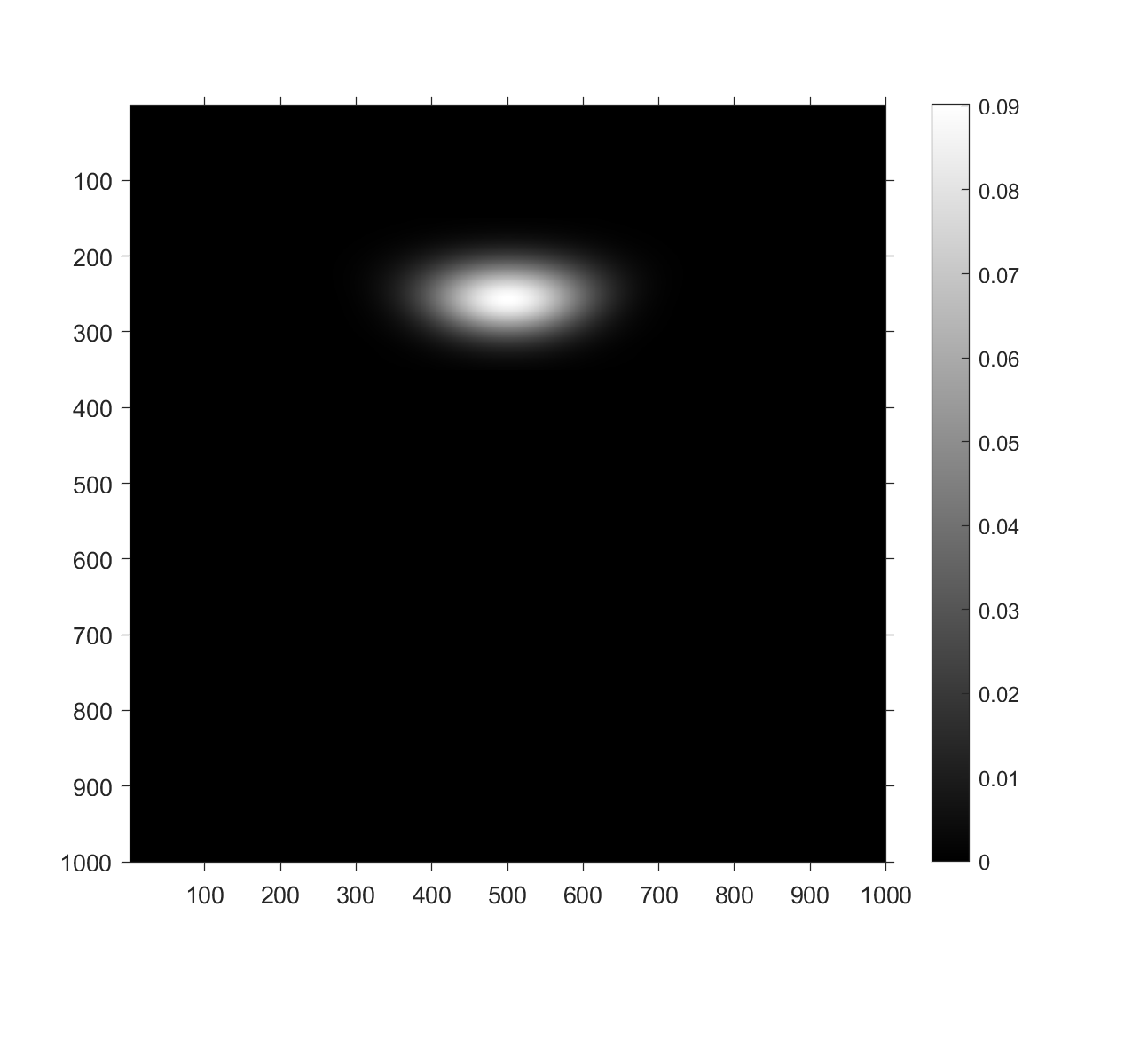
Our setup is the following. We take $n=2$ and solve (1.1) in the square $[-1,1]^{2}$ discretized into a $1,000\times 1,000$ mesh. For $\alpha$, we take an elliptic Gaussian centered at the origin with maximal value $1$ (i.e., not normalized for unit integral):

We take a plane wave starting at the bottom of the picture with corresponds to (1.3) with $\chi$ another (1D) Gaussian

where $K>0$ controls the size of the initial data, see also (3.7). We refer to Figure 1 for an illustration. We take $K$ “not too far” from $K=1$ because if $K$ is too large or too small, we are entering a different regime effectively. The regimes are defined as asymptotic ones; and we are taking only a few values of $h$. We take $K=1$ first. If we take $K\gg 1$, we are in the fully non-linear regime, if $K\ll 1$, we are in the linear one.

The non-linearity $\alpha$ is “essentially supported” away from the “support” of $u_{\text{\rm in}}$ at $t=0$ (we shift $t$ so that $t=0$ corresponds to $t=-R=\delta$ in (1.4)) and essentially leaves the “support” of $\alpha$ at time $t=1$, see Figure 2. Then $\Lambda$ in this case maps the solution at $t=0$ to that at $t=1$, the latter localized where $\chi(-1+x\cdot\omega)$ is “essentially supported”, which is also true for the solution $u$ as well.

We take $h=0.01$ first. This $h$ is not small enough relative to the standard deviation of $\chi$ and the pattern looks a bit like a coherent state in vertical direction. We really want the wavelength to be much smaller than the “support” of $\chi$. Here it is borderline so. We do not show the linear case ($K\ll 1$). The pattern just moves upward, nothing interesting.

We take $K=1$ first, see Figure 2.

The solution at $t=1$ looks very close to that of the linear PDE. A plot of the cross-section, with that of the linear solution super-imposed reveals a very slight phase shift. In Figure 3 we show a crop of that cross-section and then

where $X\alpha(x_{1})$ is the X-ray transform of $f$ along vertical lines. The picture confirms our calculations, for example the maximal value of the blob there is very close to what the right-hand of the formula above predicts.

The maximum in (4.3) is about $0.088$. That gives us distances between the zeros of the osculations of the order of $(2\pi\pm 0.088)h$, i.e., maximal relative shift of the order of $0.88/(2\pi)\approx 0.014=1.4\%$, see (4.5). This is what we see in Figure 3.

In the next example in Figure 4, $K=5$. This is getting a bit close to the fully non-linear case. The phase shift is much more apparent now. We are multiplying by $K^{2}=25$ in (4.3) to get a relative shift $\approx 35\%$. The amplitude of the non-linear oscillations drops visibly by about 20%, which is an effect that can be explained either by the next term in the expansion or by the fact that we are getting closer to the fully non-linear regime.

We decrease $h$ now by half: $h=0.005$. Then the reflection above disappears, and the relative shift is similar, see Figure 5. The phase shift computed by (4.3) looks pretty much like in Figure 3, left, but even more symmetric, with maximal value $2.1-2.2$, which is what that formula predicts. We are mainly in the weakly non-linear regime now. If we take $h$ even smaller, we are really there, of course, regardless of the value of $K$ which stays fixed.

As a test, one can plot $|u(t,x)|$ and compare that to the linear solution which is just $u_{\text{\rm in}}|_{t=1}$. If the approximation (3.6) is a good one, one should not see the non-linear effect (up to an $O(h)$ error) because the latter is in the phase only. In this case, it is almost not-visible (plot not shown), i.e., the absolute values of the linear and the non-linear solutions are very close, which is a good confirmation.

For numerical purposes it is good to integrate the phase shift (4.3) w.r.t. $x_{2}$ over $\supp\chi$ instead of fixing $x\cdot\omega=R$ (in this case, taking $x_{2}=1$) as in (3.7). This corresponds to integral in vertical direction over the top $1/3$ or so in Figure 5, for example. Then we get a multiple of $X\alpha$:

where “Data” is (4.3) integrated in $x_{2}$. In Figure 6, we show a plot of the theoretical data vs. the computed one, with $K=5$ and $h=0.005$. There is a very close match.

It follows from (3.6) that the absolute phase shift is

Recall that in (2.1) we have the prefactor $Kh^{-1/2}$ because of (4.2). For $h\ll 1$, the absolute phase shift tends to zero. If $\alpha=0$, the fundamental quasi-period is $2\pi h$. Therefore, the relative phase shift is

which is $h$-independent. The negative sign says that the wave “speeds up” which we see numerically as well. Its maximum is where $-1+x\cdot\omega=1$ (for our choice of $\chi$), i.e., at the center of the outgoing wave, and this can be observed numerically as well, see Figure 5, right.

We take $\alpha$ to have be the Shepp-Logan phantom, blurred a bit. It occupies the $[-0.5,0.5]^{2}$ square in $[-1,1]^{2}$, see Figure 7. On the right, we plot the X-ray transform along vertical lines as computed by the phase shift (in red) vs. the theoretical one in blue. One can see the Gibb’s phenomenon (or aliasing) since the wavelength is not small enough to capture the boundary. This is quite clear by just plotting the waves and the phantom one over the other. The analysis of the needed wavelength, related to the frequency content of the phantom, would be complicated since for very sharp boundaries, one can see diffraction affects. In any case, if the phantom is smooth (which it is), as $h\to 0$, we would get an accurate approximation.

Theorem B.2 illustrates that the direct problem is stable under small perturbations of the initial conditions. In the next example, we add $10\%$ noise (relative to the maximal value) to the initial condition (1.3). The waves propagate without blowing up and look weakly affected by the noise (plot not shown). In Figure 8, we plot the theoretical shift in blue computed by (4.4) vs. the computed one in red.

We choose a $2,000\times 2,000$ grid discretizing $[-1,1]^{2}$, with $h=0.0025$, $K=1$ and the phantom shown below. We take the data by rotating the image by 1 degree from $0$ to $179$ degrees. Then we extract $X\alpha$ and invert $X$. The result is shown in Figure 9. The non-linearity is included in $[-0.4,0.4]^{2}$, and this is what we plot. One can see that the resolution is relatively low, and the reconstructed image is blurred more than the original. The wavelength is approximately $2\pi h\approx 0.016$, so the displayed squares are approximately $51\times 51$ in wavelength units. Full analysis of the resolution of this method however is well beyond the scope of this paper. If we choose $\alpha$ with sharper edges (but still not with jumps), we observe diffraction effects of the waves from them. When $h\ll 1$ those effects would disappear but the computational cost then becomes too high.

When the Cauchy data $\mathbf{u}(0)$ is real valued, the solution is real and the PDE can be written as

In some works, this is the form of the semilinear wave equation with cubic non-linearities. One may think of real valued solutions being the physical ones in certain applications. We take incoming waves of the kind

Since there is no principle of superposition, we cannot take $\cos$, then $\sin$ functions above and generate the solution with the complex incoming wave (1.3). It is known that in this case we get non-trivial harmonics corresponding to values of $k$ below different from $|k|=1$, see for example [18]. The cubic type of non-linearity we have generates odd harmonics only. In Figure 10 we plot the power spectrum of a vertical slice of $u(1,x)$ with a non-linearity $\alpha$ as in (4.1); one can clearly see the peaks created by the harmonics with $|k|=1,3,5$. The higher order ones cannot be realized with the chosen level of discretization.

The weakly non-linear ansatz in this case is of the type $u=U(\phi/h,t,x,\omega,h)$ with $U$ periodic in its first variable of period, say, $2\pi$, see, e.g., [18]. Expanding the oscillatory factor in Fourier series, we assume

compare with (2.1), where each $a^{(k)}$ has an expansion $a^{(k)}=a^{(k)}_{0}+ha^{(k)}_{1}+\dots$. Using (2.3), we see that we can take the phase $\phi$ satisfying the same eikonal equation (2.4); and we take the phase $\phi=-t+x\cdot\omega$ because this is what is dictated by the initial condition (5.1). Plug (5.2) into the equivalent of (2.3) (no absolute value in $|u|^{2}$ there) to get

To simplify the notation, we will set $\mathsf{a}_{k}=a_{0}^{(k)}$. The first order transport equation derived from (5.3), in the characteristic coordinates $(s,y)$, see (3.4) and (3.5), takes the form

with initial conditions

Multiply (5.4) by $\mathsf{a}_{-k}$ and then do the same with $k$ and $-k$ swapped, subtract and sum up to get

In the last step we made the change of variables $k^{\prime}=-k$ in the last sum. If we assume uniqueness, we must have $\mathsf{a}_{k}=\bar{\mathsf{a}}_{-k}$ as can be expected because the solution (5.2) should be real valued. Indeed, take the complex conjugate of (5.4), replace $k$ by $-k$; and we get the same system of equations for $\bar{\mathsf{a}}_{-k}$. Then we get the conservation law

This means that we can look for a solution in what is essentially an $H^{1/2}$ space, see Appendix A, where we analyze the transport equations.

We can always assume that the initial condition in (5.5) is given at $s=0$. It is enough to solve (5.4) with $\alpha=1$. Indeed, let that solution be $\tilde{\mathsf{a}}$; then $\mathsf{a}(s)=\tilde{\mathsf{a}}(\mathcal{R}(s))$ solves (5.4) with $\mathcal{R}(s)=\int_{0}^{s}\alpha(\sigma)\,\mathrm{d}\sigma$. In particular, if $\alpha=0$, we get $\mathsf{a}(s)=\tilde{\mathsf{a}}(0)$, which is the vector with only two non-zero components as in (5.5). Notice that for $s=T$, the value of $s$ at which the ray has exited $\overline{B(0,R)}$, $\mathcal{R}(T)=\int\alpha$ is the X-ray transform of $\alpha$ in the direction of $\omega$. In fact, the measurements provide $\mathsf{a}_{k}(T)$ for all $k$. They equal $\tilde{a}_{k}(\mathcal{R}(T))$. If this function is invertible for at least one $k$, we recover $\mathcal{R}(T)$, and therefore the X-ray transform of $\alpha$. By the ODE system (5.4) and (5.6) (or by uniqueness), we cannot have $\mathrm{d}\tilde{\mathsf{a}}_{k}/\mathrm{d}s=0$ for all $k$ and a fixed $t$ (recall that $\alpha=1$ for $\tilde{a}$). Therefore, at least locally, we can invert one of those functions. We show below that this can be done for small $\alpha$.

Note that we can view the argument above as a version of the phase shift we encountered with complex probing waves. The change of variables $s\mapsto\mathcal{R}(s)$ along each characteristic line, having non-negative derivative $\alpha$, deforms $\tilde{\mathsf{a}}(s)$ to $\mathsf{a}(s)=\tilde{\mathsf{a}}(\mathcal{R}(s))$. We cannot expect each $\mathsf{a}_{k}$ to have a constant module as in (3.3), then this change will shift both the phase and the amplitude.

Since it is not clear if (5.4) can be solved explicitly with $\alpha=1$, we will linearize the solution near $\alpha=0$. If $\alpha=0$, the solution is $\mathsf{a}^{0}=(Ae_{-1}+Ae_{1})/2$ with the standard notation $e_{k}$ for the vector with all components zero except at the $k$-th position, which is $1$. The linearization $\delta\mathsf{a}$ at $\alpha=0$ is given by

The only non-zero coefficients correspond to $k=-3,-1,1,3$. It is easy to see that

Therefore, the first order approximation to the r.h.s. of (5.2) without the factor $h^{-1/2}$ about $\alpha=0$ is

where $\mathcal{R}=\int_{-\infty}^{0}\alpha(x+s\omega)\,\mathrm{d}s$, and $A=\chi(-t+x\cdot\omega)$, compare to (3.5). The first term in (5.7) is just the linear solution $u_{L}$, therefore the linearization $\delta u$ is $\delta u=u_{1}-u_{L}$.

Motivated by this, we take our data to be $\delta u$ at $t=T$, and $x\cdot\omega=T+h\pi/2$ to get $K^{3}\mathcal{R}/3$ (up to an $O(h)$ error), with $K=\chi(0)$ as before, which recovers $\mathcal{R}$. For numerical purposes, it is better to integrate $|\delta u|^{2}|_{t=T}$ over an $h$-independent range of $x$ values lying away from $\supp\alpha$:

Here $\mathcal{R}=X\alpha$ is the X-ray transform of $\alpha$ in the direction $\omega$. The product $C\sin(\sigma/h)\sin(3\sigma/h)$ is missing because it is $O(h^{\infty})$ as it can be seen by writing it as a difference of cosine functions and integrating by parts. Now, since $\sin^{2}\beta=(1-\cos(2\beta))/2$, the contribution of each sine squared term above would be $1/2+O(h^{\infty})$, hence

References

- [1] J.-M. Bony. Interaction des singularités pour les équations aux dérivées partielles non linéaires. In Goulaouic-Meyer-Schwartz Seminar, 1981/1982, pages Exp. No. II, 12. École Polytech., Palaiseau, 1982.
- [2] J.-M. Bony. Second microlocalization and propagation of singularities for semilinear hyperbolic equations. In Hyperbolic equations and related topics (Katata/Kyoto, 1984), pages 11–49. Academic Press, Boston, MA, 1986.
- [3] P. Brenner. On the existence of global smooth solutions of certain semilinear hyperbolic equations. Math. Z., 167(2):99–135, 1979.
- [4] I. Dajani, G. DiPeso, E. Morse, and R. Ziolkowski. Gaussian beam propagation in a weakly nonlinear medium: A geometrical optics approach. Physical review. A, Atomic, molecular, and optical physics, 41(7):3740–3745, 1990.
- [5] I. Dajani, E. Morse, and R. Ziolkowski. Weakly nonlinear geometrical optics in plasmas. Physica D: Nonlinear Phenomena, 64(1-3):237–250, 1993.
- [6] B. Dodson. Global well-posedness for the radial, defocusing, nonlinear wave equation for . arXiv preprint arXiv:1810.02879, 2018.
- [7] P. Donnat and J. Rauch. Dispersive nonlinear geometric optics. J. Math. Phys., 38(3):1484–1523, 1997.
- [8] E. Dumas. About nonlinear geometric optics. Bol. Soc. Esp. Mat. Apl. SeMA, (35):7–41, 2006.
- [9] Y. Ebihara. Nonlinear Cauchy problem for hyperbolic type equations. Mem. Fac. Sci. Kyushu Univ. Ser. A, 26:156–173, 1972.
- [10] E. Heinz and W. von Wahl. Zu einem Satz von FE Browder über nichtlineare Wellengleichungen. Mathematische Zeitschrift, 141(1):33–45, 1975.
- [11] P. Hintz and G. Uhlmann. Reconstruction of Lorentzian manifolds from boundary light observation sets. Int. Math. Res. Not. IMRN, (22):6949–6987, 2019.
- [12] J.-L. Joly, G. Métivier, and J. Rauch. Coherent and focusing multidimensional nonlinear geometric optics. Ann. Sci. École Norm. Sup. (4), 28(1):51–113, 1995.
- [13] J.-L. Joly and J. Rauch. Justification of multidimensional single phase semilinear geometric optics. Trans. Amer. Math. Soc., 330(2):599–623, 1992.
- [14] K. Jörgens. Das Anfangswertproblem im Grossen für eine Klasse nichtlinearer Wellengleichungen. Math. Z., 77:295–308, 1961.
- [15] Y. Kurylev, M. Lassas, and G. Uhlmann. Inverse problems for Lorentzian manifolds and non-linear hyperbolic equations. Invent. Math., 212(3):781–857, 2018.
- [16] M. Lassas, G. Uhlmann, and Y. Wang. Inverse problems for semilinear wave equations on Lorentzian manifolds. Comm. Math. Phys., 360(2):555–609, 2018.
- [17] R. Melrose and N. Ritter. Interaction of nonlinear progressing waves for semilinear wave equations. Ann. of Math. (2), 121(1):187–213, 1985.
- [18] G. Métivier. The mathematics of nonlinear optics. In Handbook of differential equations: evolutionary equations. Vol. V, Handb. Differ. Equ., pages 169–313. Elsevier/North-Holland, Amsterdam, 2009.
- [19] G. Métivier, J.-L. Joly, and J. Rauch. Recent results in non-linear geometric optics. In Hyperbolic problems: theory, numerics, applications, Vol. II (Zürich, 1998), volume 130 of Internat. Ser. Numer. Math., pages 723–736. Birkhäuser, Basel, 1999.
- [20] L. Oksanen, M. Salo, P. Stefanov, and G. Uhlmann. Inverse problems for real principal type operators. arXiv preprint arXiv:2001.07599, 2020.
- [21] M. Reed and B. Simon. Methods of modern mathematical physics. II. Fourier analysis, self-adjointness. Academic Press [Harcourt Brace Jovanovich, Publishers], New York-London, 1975.
- [22] A. Sá Barreto. Interactions of semilinear progressing waves in two or more space dimensions. Inverse Probl. Imaging, 14(6):1057–1105, 2020.
- [23] A. Sá Barreto and Y. Wang. Singularities generated by the triple interaction of semilinear conormal waves. arXiv:1809.09253, page 34, 2018.
- [24] I. Segal. Non-linear semi-groups. Ann. of Math. (2), 78:339–364, 1963.