A structural approach to default modelling with pure jump processes
Abstract
We present a general framework for the estimation of corporate default based on a firm’s capital structure, when its assets are assumed to follow a pure jump Lévy processes; this setup provides a natural extension to usual default metrics defined in diffusion (log-normal) models, and allows to capture extreme market events such as sudden drops in asset prices, which are closely linked to default occurrence. Within this framework, we introduce several pure jump processes featuring negative jumps only and derive practical closed formulas for equity prices, which enable us to use a moment-based algorithm to calibrate the parameters from real market data and to estimate the associated default metrics. A notable feature of these models is the redistribution of credit risk towards shorter maturity: this constitutes an interesting improvement to diffusion models, which are known to underestimate short term default probabilities. We also provide extensions to a model featuring both positive and negative jumps and discuss qualitative and quantitative features of the results. For readers convenience, practical tools for model implementation and GitHub links are also included.
Keywords: Lévy process; Gamma process; Inverse Gaussian process; One-sided process; Variance Gamma process; Credit risk; Distance to default; Default probability.
AMS subject classifications (MSC 2020): 60E07, 60E10, 62P05, 91G30, 91G40.
JEL Classifications: C02, G12, G32.
1 Introduction
We start the paper by providing a general introduction to the so-called structural approach to credit risk, recalling the main limitations of log-normal models and introducing the more realistic class of pure jump models. We also detail the main contributions of the paper in this context, as well as its overall structure.
1.1 Structural modelling, credit spread puzzle and jump risk
A popular approach to credit risk and corporate default modelling is to assume that the value of a firm’s assets is driven by a certain stochastic dynamics, and that a default occurs when the realization of this process is lower than the facial value of the firm’s debt at its maturity. This approach, which has been called the structural approach by Duffie & Singleton 1999, was pioneered by the works of Black & Scholes 1973 and Merton 1974, the authors introducing a diffusion process to model the underlying asset log returns; this setup is now universally known as the Merton model, and has subsequently been extended to take into account various features, such as the existence of multiple maturities for the firm’s debt (Geske 1977) or the possibility for the default to occur prior to the debt’s maturity (Black & Cox 1976; Longstaff & Schwartz 1995; Leland & Toft 1996); these latter models are often referred to as first passage or barrier models. Extensions to sovereign issuers have also been considered (Gray & al. 2007). For a complete overview of default modelling and related topics within the structural approach (as well as in the alternative class of reduced-form models), we refer to Duffie & Singleton 2012; Lipton & Rennie 2013.
A major difficulty in the structural approach lies in its calibration, because most of the corporate debt is not traded and, therefore, it is not possible to obtain directly the value of a firm’s assets by summing its equity and debt values. In this context, assuming that assets log returns are driven by a diffusion process (i.e., a Wiener process, or Brownian motion) is particularly useful, because it allows for a closed-form relationship between a firm’s value and its equity, via the celebrated Black-Scholes formula. This closed formula opens the way to simple historical calibrations for the asset’s volatility, by solving a system of nonlinear equations with classical solvers such as the Newton-Raphson method in the algorithm developed by Vassalou and Xing 2004; other calibrations techniques for diffusion models have also been introduced, for instance based on the book value of the debt in Eom & al. 2004 or on maximum likelihood estimations (see details in Duan & al. 2004).
The Brownian hypothesis, however, has been severely criticized for being unrealistic and, notably, for producing an almost zero default probability for short maturities: if this was true, then short term bonds should have zero credit spread, which is typically not the case, as first noted by Jones & al. 1984 (see also many subsequent discussions such as Lyden & Saraniti 2000 or Demchuk & Gibson 2009 for instance). This underestimation of short term default probabilities and of theoretical credit spreads is known as the credit spread puzzle and has been evidenced many times and for every ranking, from high yield to investment grade issuers (see a recent overview in Huang & al. 2019) and even sovereign issuers (see Duyvesteyn & Martens 2015 and references therein). Among the plausible explanations for this discrepancy are the fact that other factors can influence credit spreads, such as taxes, liquidity premia (D’Amato & Remolona 2003) and jump risk (Bai et al. 2020).
This phenomenon is also evidenced when examining 1 year historical default rates; in 2019, the S&P global default rate (all issuers) was of 1.03%, and, on the non investment grade or speculative sector corresponding to BB ratings and lower, it reached 2.10% (Kraemer & al. 2020). With the dramatic COVID19 events, the situation has worsened, and the default rate is expected to reach 10% in 2021 on the non investment grade sector, which now represents 30 % of all issuers, at an all time high (Kraemer 2020). Such levels are similar and even higher to those following the global financial crisis (GFC) of 2007-2008 (1 year speculative default rate was of 9.94% in 2009), and cannot be obtained from the classical Merton model, in particular because the normal assumption fails to reproduce extreme market events. A natural idea is therefore to introduce jumps in the assets dynamics, in order to better capture short term defaults occurring after a brutal drop in the value of a company’s assets following, for instance, earning announcements, central bank meetings or major political events.
Jump processes can be of two kinds: jump-diffusion processes, or pure jumps processes, and both are conveniently described by the formalism of Lévy processes. Jump diffusion processes were introduced in structural credit risk modelling by Zhou 1997, by adding a Poisson process whose discrete jumps are normally distributed to the usual diffusion process, in order to materialize sudden changes in the firm’s assets value; other distributions for the magnitude of the Poisson jumps have subsequently been considered, such as negative exponential distributions in Lipton 2002, leading to higher short term probabilities and more realistic credit spread curves. Self exciting Hawkes process have also been introduced in Ma & Xu 2016, a model for which an analytical formula for the equity value has been recently derived in Pasricha & al. 2021. Pure jump processes allow for an even richer dynamics and, notably, an interpretation in terms of business time (differing from the operational time), or the possibility for jumps to occur arbitrarily often on any time interval; such processes were introduced in the construction of credit risk models in the late 2000s and early 2010s, notably in Madan & Schoutens 2008 for one-sided processes (i.e., featuring downward jumps only) and from the point of view of first passage models, and in Foriani & al. 2006; Fiorani & al. 2010; Luciano 2009 for double-sided processes, with CDS-based calibrations. Extensions to multivariate processes have also been studied (Marfè 2012).
In this paper, we would like to demonstrate that pure jump processes are well suited to the structural approach, thus confirming the initial works cited above, but also that practical formulas can be derived for the equity value, thus allowing for a precise issuer-based calibration. We will also show that incorporating realistic features such as non-normality of returns, jumps or asymmetry, allows to better capture the probability of a default occurrence in particular during turbulent times, and provides a better fit to historical default rates notably for speculative issuers. This approach appears to be particularly relevant in the current COVID19 period: as already mentioned, short term defaults are expected to increase, as they did during former major crisis (GFC, dot com crisis …). Moreover, while former peaks of default events lasted typically one or two years before going back to "usual" default rates, it is likely that, this time, the situation may last far longer, given the enormous amounts of debt that have been accumulated and the feeble revenues that most firms were able to collect between lockdown periods.
1.2 Contributions of the paper
We will focus on:
- (a)
Extending the structural approach to the case where the stochastic process is no longer a Brownian motion but a more general Lévy process, defining credit risk metrics in that context and showing how model parameters can be calibrated using observable issuers data;
- (b)
Deriving closed pricing formulas for the equity value of a firm when the Lévy process is assumed to be spectrally negative, and implementing the calibration algorithm using these formulas;
- (c)
Showing that obtained default probabilities are higher than the Merton default probabilities for short maturities, and comparing real world default probabilities with historical default rates;
- (d)
Using recent pricing formulas in the context of double-sided processes and, like in (b) and (c), discussing calibration and obtained probabilities.
1.3 Structure of the paper
In section 2, we recall basic facts on Lévy processes, we define credit risk metrics (distance to default, default probability) in this context, and we present the calibration algorithm that extends the algorithm of Vassalou and Xing 2004 to the case of pure jump processes. Then, in section 3, we introduce two spectrally negative processes which are similar to the Gamma and inverse Gaussian subordinators, but with a Lévy measure translated to the negative real axis, allowing us to define the NegGamma and NegIG credit risk models; we derive explicit formulas for equity values in these models and, using the calibration algorithm, we determine model parameters, compute default probabilities (both in the risk-neutral and real world cases) and compare them with Merton probabilities as well as with historical default rates. We proceed to a similar discussion in section 4, but for a process featuring a double-sided Lévy measure which, for simplicity, is assumed to be symmetric; equity value in this case is based on series expansions whose terms are powers of the distance to default. Section 5 is dedicated to concluding remarks and future works. For reader’s convenience, we have also equipped the paper with an appendix, which summarizes the papers notations, provides details on the data set of test issuers used in the study and on parameters stability, and contains a link to the GitHub where the calibration code can be freely accessed.
2 Pure jump asset dynamics and risk metrics
In this section, we start by recalling some fundamental concepts on Lévy processes and asset pricing (we refer to the classical references Bertoin 1996 and Schoutens 2003 for all technical details), that extend the classical log-normal Merton model. Then, we introduce the generalization of distance to default and default probability in this context, as well as the general algorithm that will be used to calibrate the various models in the rest of the paper.
2.1 Model setup
2.1.1 Model formulation
Following the classical setup of structural credit risk modelling, we consider a company possessing a total asset at time , financed by an equity and a zero coupon debt of maturity and face value :
| (1) |
At , two situations can occur:
- -
: the issuer has enough financial resource to pay off for the full amount of its debt , and in that case its equity still has a positive value equal to ;
- -
: the company is in default, and in that case its equity value falls down to .
In short, we see the equity value of a firm as a European call option written on its assets, whose strike price (resp. maturity) equals the face value (resp. the maturity) of the company’s debt; following the usual financial notation, we will therefore write that
| (2) |
We deliberately use a European formulation instead of a first passage one, which, at first sight, could appear more precise as default can occur at all . The reason is that our purpose is to find a good balance between realistic features (presence of brutal market events, materialized by a pure jump dynamics for ), and computational tractability (allowing for a simple issuer-based calibration procedure, necessitating only observable equity prices). If we had chosen a first passage formulation, then the equity price (2) would have become a barrier option, for which a simple closed formula exists if is log-normal, but not if it follows a purely discontinuous process, depriving us for a simple calibration algorithm based on the inversion of an equity formula. Extending pricing formulas for barrier options to the case of pure jump processes is, actually, an interesting subject in itself and could be made possible at least in the -stable case by using a generalization of the reflection principle (see Bingham 1973) which states that, if follows an -stable process (), then
| (3) |
which degenerates into the usual Brownian principle when . But, as stable distributions have infinite moments except for the degenerate case , we would be unable, again, to use a simple moment matching procedure to calibrate model parameters. On the contrary, focusing on a European approach but combining this simple approach with some well-chosen pure jump processes (for which we will be able to derive closed formula for equity prices), will allow to combine both the advantages of computational simplicity and realistic description of the assets behaviour.
As we will see in the next sections, the pure jump Lévy processes we will introduce to model the dynamics of will mainly be spectrally negative (that is, feature downward jumps only) because it is this skewed behaviour that has the biggest impact on the credit risk of a firm. The main intuition behind this is that, even if we measure default probability only at , downward jumps (materializing a sudden drop in assets value) can occur anytime in ; if such a jump occurs not too far from maturity, and if no positive jumps are allowed, then it will not be possible for asset prices to grow up to the debt level before maturity and default will almost surely occur. For sake of generality, we will also extend the study to the case of a symmetric process.
Let us mention that more general pure jump processes have already been considered for the purpose of default modelling (for instance the Variance Gamma process, see Fiorani & al. 2010), featuring one or more supplementary degree of freedom (allowing, for instance, to control the asymmetry of tails). But, for such processes, no simple closed formula can be derived for equity prices, and calibration is typically performed using CDS; as they are not traded for every name and maturity, one has to use CDS indices as proxies. On the contrary, the main novelty of our approach is that we are able to derive convenient closed-form equity formulas, which opens the way to a simple calibration algorithm that only necessitates equity prices as input; the Lévy processes involved are less sophisticated than an asymmetric Variance Gamma process, but remain far more realistic than the usual diffusion approach.
2.1.2 Dynamics
We will assume that, given a filtered probability space , the instantaneous variations of the firm’s assets can be written down in local form as
| (4) |
under an admissible equivalent martingale measure (EMM), or risk-neutral (RN) measure, traditionally denoted by (see discussion thereafter in subsection 2.3). In (4), is the (continuously compounded) risk-free interest rate and is a Lévy process, that is, a càdlag process satisfying (-almost surely), and whose increments are independent and stationary. Note that when where is a centered Wiener process, then follows a geometric Brownian motion, and in that case (4) corresponds to the traditional Merton model.
The solution to the stochastic differential equation (4) is the exponential process
| (5) |
where and where is a convexity adjustment computed in a way that the discounted asset prices are a -martingale, i.e.
| (6) |
As is a Lévy process, its probability distribution is infinitely divisible and, consequently, its characteristic function admits a semigroup structure. In other words, there exists a function called characteristic exponent, or Lévy symbol, such that , and which is entirely characterized by the Lévy-Khintchine formula
| (7) |
where is the drift and is the Brownian (or diffusion) component. The measure , assumed to be concentrated on and satisfy
| (8) |
is called the Lévy measure of the process, and determines its tail behaviour and the distribution of jumps. If and the Lévy measure has finite total mass, one speaks of a jump-diffusion process and in that case only a finite number of jumps can occur on any finite time interval; among the most popular distributions for the random size of jumps are Gaussian distributions (Zhou 1997) or exponential distributions (Lipton 2002). Non-random discrete (Dirac) jumps have also been introduced in Lipton & Sepp 2009, and shown to provide remarkably good results when implemented in a model featuring multi-name joint dynamics, notably because they allow to achieve higher levels of correlations than exponential jumps. Among other jump-diffusion models, let us also cite the works by Hilberink & Rogers 2002 or Le Courtois & Quittard-Pinon 2006 (which is the credit risk counterpart of the geometric Kou model (Kou 2002) for option pricing). When , one speaks of a pure jump process and, if furthermore , we say that the process has infinite activity (or intensity). For such processes, an infinite number of jumps can occur on any time interval, making for a very rich and complex dynamics; among the most prominent pure jump Lévy processes are the so-called subordinators (i.e. models for which ) such as the Gamma or Inverse Gaussian processes, or models featuring both positive and negative jumps such as the Variance Gamma (VG) process (Madan et al. 1998) or the Normal Inverse Gaussian (NIG) process (Barndorff-Nielsen 1995; Barndorff-Nielsen 1997). Let us also mention that the drift actually depends on the choice of the so-called truncation function (in (7) we choose , but the choice is not unique), and therefore can be eliminated by a suitable choice of truncation. Last, let us remark that, as a direct consequence of the definition of the Lévy symbol, the condition (6) can be reformulated as:
| (9) |
Remark 1.
If where is a centered Wiener process, it is well known that . From the point of view of the representation (7), this means that the Lévy measure is identically null and that the Lévy symbol resumes to its diffusion component i.e. ; it results that the convexity adjustment in this case is
| (10) |
which is the usual Gaussian (Black-Scholes-Merton) adjustment.
Let us now introduce the quantity
| (11) |
which, in the context of option pricing, is generally called the log forward moneyness, and let us denote by the density of the process . Then, we can formulate a proposition:
Proposition 2.1 (Equity value).
Under the dynamics (4), the equity value of a firm can be written as
| (12) |
Proof.
From (2) and the standard theory of martingale pricing, the value of a firm’s asset is
| (13) |
Using (5) and the notation (11), we can re-write (13) as
| (14) |
The last expectation can be carried out by integrating all possible realizations for the terminal payoff over the process density, resulting in formula (12). ∎
Remark 2.
In the standard option pricing theory, the risk-neutral (martingale) representation formula (13) holds true only if the firm’s assets (materialized by the process ) are tradeable, which, in general, is not the case. According to Ericsson & Reneby 2002, the approach is still licit because it is possible to constitute a portfolio of traded assets that possesses exactly the same dynamics than ; in other words, even if cannot be traded, it can be replicated by a tradeable portfolio, and, therefore, the models can still be based on the risk-neutral representation (which, in the case of a Lévy process, is not necessarily unique, see further discussion in section 2.3).
2.2 Risk-neutral distance to default and default probabilities
The occurrence of a default at time corresponds to the situation where the value of the firm’s asset is lower than the facial value of the debt; in this situation, the firm’s equity becomes equal to 0 and, therefore, it follows from eq. (14) that the probability of such an event is
| (15) | ||||
| (16) |
where is the cumulative distribution function of the process evaluated at :
| (17) |
These observations motivate the following definitions:
Definition 1 (Risk-neutral Default Metrics).
- 1.
Under the pure jump dynamics (4), the risk-neutral distance to default of a firm is defined to be
(18) - 2.
The corresponding risk-neutral default probability of the firm is defined to be
(19)
Example 1 (Merton model).
If where , then the process admits the following density (heat kernel):
| (20) |
The cumulative distribution function is therefore
| (21) |
where is the cumulative distribution function of the standard normal distribution . It follows from remark 1 and definition 1 that the risk-neutral default probability is
| (22) |
where (following the usual Black-Scholes notation) is often interpreted as the risk-neutral distance to default in the Merton model.
2.3 Actual (real-world) distance to default and default probabilities
The metrics introduced in definition 1 are risk-neutral metrics, because in equation (4) we have chosen to specify the dynamics for directly under the risk-neutral, or martingale measure . To be fully rigorous, let us mention that is unique only if the market is complete and that, when Lévy processes are involved, the market is in general incomplete; this means that several equivalent martingale measures exist, and that the choice (9) is not unique - this is however the standard choice (see details e.g. in Schoutens 2003). We may note that, using the notations defined in appendix A, equation (9) can be re-formulated in terms of the cumulant generating function as
| (23) |
allowing to define our choice for the change of measure via the following Radon-Nikodym derivative
| (24) |
Under this definition, the measure is sometimes referred to as the exponentially tilted measure, or the Esscher transform of the physical measure.
Risk-neutral default probabilities can be used as a convenient proxy for the estimation of actual (also called physical, or real-world) default probabilities, as they essentially convey the same information and sensitivities to the variables such as debt or model parameters (see a discussion e.g. in Delianedis & Geske 2003); moreover, they are well-suited to derivatives-based calibrations (such as CDS quotes), and it is common market practice that xVA calculations are commonly made under the measure (Gregory 2015). However, the risk-free rate in the dynamics (4) generally differs from the actual drift at which the assets grow11 1 The actual drift is often denoted by in the literature; we do not use this notation, in order to avoid confusion with the mean parameter for the inverse Gaussian subordinator and the standardized central moments., and computing actual default probabilities can be necessary if one wishes to perform precise default computations, in particular in the framework of portfolio exposure (see for instance a discussion in Stein 2016); in this context, instead of specifying the dynamics 4 under the -measure, we can choose to specify it under the real-world measure and, doing so, to replace the risk-free rate is by the actual drift ; the analogue to the risk-neutral metrics 1 are the actual (or real-world) risk metrics
| (25) |
from which it follows that risk-neutral and actual default probabilities coincide only if (that is, if the underlying assets grow at exactly the risk-free rate). In subsection 2.4, we will explain how both model parameters and actual drift can be calibrated using historical data and a moment-matching algorithm.
2.4 Historical calibration algorithm
2.4.1 Model parameters
Given a period of consecutive trading days , with, for simplicity, constant spacing for all , we constitute a time-series of realizations of the log-returns of ; using (5), it can be written as
| (26) |
In our applications, we will choose a constant spacing parameter , i.e., daily data, but other choices of data frequency are of course possible. We denote by the set of moments of order greater than 2 of (see definitions (92) and (93) in appendix A). We assume that the model has parameters (or equivalently, that the process has degrees of freedom) grouped in a set denoted by , and we choose a subset of moments of of order greater than 2; we assume that the moments of are known in terms of the model parameters, that is, that we can write for some bijective function . Last, we assume that, using proposition 2.1, we were able to derive a closed pricing formula for the equity price, that is, that we have found a locally invertible function such that
| (27) |
Note that we focus on the dependence on the model parameters but of course the function can also depend on other external parameters such as maturity or debt level for instance. The purpose of algorithm 1 is to determine (seen as a vector) as the limit of a sequence of vectors calibrated from observable market data, i.e., formally,
| (28) |
Algorithm 1 (Calibration).
- (1)
Choose real numbers, group them under the form of a vector and, for each date , define
(29) - (2)
Denote and its associated subset of moments of order greater than 2, and define
(30) - (3)
Repeat step (1) and (2): introduce
(31) and the subset of moments of order greater than 2 of , and define
(32) - (4)
Stop the algorithm once a desired level of precision is attained, e.g. .
2.4.2 Actual drift
When it comes to estimating actual (real world) default probabilities, algorithm 1 remains valid but we have, furthermore, to estimate the actual drift . We note that, under the measure, the series of log returns (26) becomes
| (33) |
and, therefore, the associated first order moment (the mean) reads
| (34) |
where the convexity adjustment depends on the model parameters that have been calibrated in algorithm 1. It follows immediately that
| (35) |
Remark 3.
In the Merton case, choosing , we have and and therefore
| (36) |
3 One-sided models
In this section, we will be particularly interested in the case where the Lévy process in (4) is spectrally negative, that is, features negative (downward) jumps only; this will lead us to introduce two spectrally negative pure jump processes, namely the NegGamma and NegIG processes. Let us note that one-sided processes have already been applied to default modelling, e.g. in Madan & Schoutens 2008, but from a point of view of negative subordinators, and with a first passage time approach and a CDS-based calibration. Our approach is different: we will first establish closed formulas for the equity value of the firms under these dynamics and show how they can be used for historical issuer-based calibrations and estimation of default probabilities.
3.1 Negative Gamma (NegGamma) credit risk model
We define the NegGamma process to be the pure jump process whose Lévy measure reads
| (37) |
for some positive real numbers and ; within this parametrization is called the rate parameter, and the shape parameter. It follows from the Lévy-Khintchine representation (7) that the Lévy symbol of the NegGamma process is, with an adapted choice of truncation function,
| (38) |
The cumulant generating function is therefore
| (39) |
from which we easily deduce the cumulants (see further details e.g. in Küchler & Tappe 2008). In particular, we obtain, for the standardized moments of the log returns ():
| (40) |
3.1.1 Default metrics
It follows from (38) that the martingale adjustment for the NegGamma process is
| (41) |
and therefore the distance to default is
| (42) |
The characteristic function also follows immediately from (38):
| (43) |
and, inverting this Fourier transform, we get the density function
| (44) |
from which we obtain the cumulative distribution function:
| (45) |
where stands for the upper incomplete Gamma function (see appendix A and Abramowitz & Stegun 1972). As a consequence of definition 1, the default probability of a firm thus writes
| (46) |
As a consequence of the definition of the upper incomplete Gamma function, it is clear that when , and that there is a 100% default probability as soon as the distance to default is null or negative. In other words, there is no more chance for to be greater than as soon as , which is a consequence of the occurrence of downward jumps only.
3.1.2 Equity value
Let denote the lower incomplete gamma function, such that the equality holds for all .
Proposition 3.1.
The equity value of a firm in the NegGamma credit risk model can be written as:
| (47) |
Proof.
3.1.3 Parameter calibration
There are 2 parameters to calibrate (, and , and therefore it suffices to use two central moments in algorithm 1, for instance the variance and excess kurtosis . Given the formulas (40), we introduce the function
| (50) |
Let denote the time series of observable prices during a one year period preceeding the calculation date, and let us initiate we initiate algorithm 1 by choosing . Following algorithm 1, we have to evaluate which can be performed via a classical Newton-Raphson algorithm for the pricing formula in proposition 3.1, while the function is straightforward to obtain from definition (50). Calibration results are displayed in table 1 for a data set constituted of investment grade and speculative issuers with various rankings (see details in table 8 in appendix B); speed of convergence (typical number of steps needed for algorithm 1 to converge) is discussed in table 5, and stability of the parameters is discussed in appendix C.
| NegGamma model | Merton model | |||||
|---|---|---|---|---|---|---|
| (in MM) | (in MM) | (in MM) | ||||
| SAP GY | 16 196 | 180 913 | 3.280 | 0.888 | 180 914 | 28.73% |
| MRK GY | 14 180 | 70 763 | 3.224 | 0.645 | 70 766 | 24.87% |
| AI FP | 14 730 | 78 928 | 3.194 | 0.559 | 78 931 | 23.40% |
| SU FP | 8 473 | 71 471 | 2.200 | 0.510 | 71 474 | 32.45% |
| CRH LN | 10 525 | 33 935 | 2.700 | 0.684 | 33 965 | 30.38% |
| DAI GY | 161 780 | 213 453 | 6.736 | 0.530 | 214 039 | 10.78% |
| VIE FP | 16 996 | 27 243 | 4.102 | 0.452 | 27 319 | 16.14% |
| SRG IM | 14 774 | 29 527 | 2.834 | 0.310 | 29 585 | 19.38% |
| AMP IM | 1 339 | 8 627 | 1.784 | 0.414 | 8 629 | 35.95% |
| FR FP | 4 879 | 11 379 | 2.746 | 0.774 | 11 415 | 31.98% |
| EO FP | 4 838 | 9 993 | 3.786 | 1.129 | 10 023 | 27.75% |
| GET FP | 4 498 | 11 658 | 3.230 | 0.612 | 11 675 | 23.98% |
| LHA GY | 10 106 | 14 635 | 4.074 | 0.784 | 14 730 | 21.61% |
| PIA IM | 609 | 1 491 | 4.138 | 1.050 | 1 492 | 24.54% |
| CO FP | 14 308 | 16 445 | 11.896 | 0.745 | 16 494 | 7.11% |
3.2 Negative Inverse Gaussian (NegIG) credit risk model
We define the NegIG process to be the pure jump process whose Lévy measure reads
| (51) |
for some positive real numbers (shape) and (mean); from the Lévy-Khintchine representation (7), we deduce the Lévy symbol for the NegIG process:
| (52) |
The cumulant generating function is therefore
| (53) |
from which we easily deduce the cumulants and the corresponding central moments:
| (54) |
3.2.1 Default metrics
It follows from (52) that the martingale adjustment for the NegIG process is
| (55) |
and therefore the distance to default is
| (56) |
The characteristic function also follows immediately from (52):
| (57) |
and, inverting this Fourier transform, we get the density function
| (58) |
From definition 1 and Shuster’s integrals (see (86) in appendix A), we therefore obtain the default probability in the negIG model:
| (59) |
where N(.) stands for the standard normal cumulative distribution function (see apprendix A).
3.2.2 Equity value
Let us define the function
| (60) |
Proposition 3.2.
The equity value of a firm in the NegIG credit risk model can be written as:
| (61) |
Proof.
If , then using proposition 2.1 with the density (58), and changing the variable , we can write the equity value as:
| (62) |
The second integral can be performed directly from formula (86) and the definition of the function; the first integral can be carried out in a similar way, after completing the square
| (63) |
and recalling that
| (64) |
Last, if , then and therefore the integral (12) is equal to zero as the density (58) is supported by the real negative axis only. ∎
3.2.3 Parameter calibration
Calibration process for the NegIG parameters and goes like the NegGamma calibration in sub-subsection 3.1.3, by using variance and excess kurtosis, and by introducing the function
| (65) |
whose inverse is straightforward to compute.
3.3 Comparison of default probabilities and discussion
3.3.1 Risk-neutral default probabilities
In table 2, we compare the risk-neutral default probabilities obtained for the set of issuers (see details in appendix B) with our NegGamma and NegIG models, to the one obtained via the classical Merton model, for two distinct horizons (1 year and 5 years).
| Rating | Category | NegGamma | NegIG | Merton | ||||
| = 1 y. | =5 y. | = 1 y. | =5 y. | =1 y. | =5 y. | |||
| SAP GY | A | Inv | 0.01% | 0.47% | 0.01% | 0.46% | 0.00% | 0.03% |
| MRK GY | A | Inv | 0.12% | 1.90% | 0.12% | 1.84% | 0.00% | 0.47% |
| AI FP | A- | Inv | 0.08% | 1.26% | 0.08% | 1.22% | 0.00% | 0.16% |
| SU FP | A- | Inv | 0.14% | 2.02% | 0.14% | 1.95% | 0.00% | 0.51% |
| CRH LN | BBB+ | Inv | 1.10% | 10.11% | 1.02% | 9.97% | 0.01% | 10.85% |
| SRG IM | BBB+ | Inv | 1.73% | 10.53% | 1.56% | 10.27% | 0.02% | 11.04% |
| DAI GY | BBB+ | Inv | 3.26% | 20.94% | 3.00% | 21.06% | 0.55% | 34.13% |
| VIE FP | BBB | Inv | 2.62% | 14.96% | 2.39% | 14.77% | 0.21% | 17.14% |
| AMP IM | BB+ | Spec | 0.50% | 4.82% | 0.47% | 4.66% | 0.00% | 3.16% |
| FR FP | BB+ | Spec | 3.12% | 21.63% | 2.90% | 21.84% | 0.62% | 33.48% |
| EO FP | BB | Spec | 3.06% | 22.02% | 2.87% | 22.13% | 0.65% | 29.00% |
| GET FP | BB- | Spec | 1.50% | 11.43% | 1.38% | 11.26% | 0.03% | 12.11% |
| LHA GY | BB- | Spec | 7.29% | 34.11% | 6.93% | 34.67% | 5.09% | 49.57% |
| PIA IM | B+ | Spec | 1.08% | 11.22% | 1.02% | 11.10% | 0.02% | 11.66% |
| CO FP | B | Spec | 5.62% | 24.97% | 5.29% | 24.94% | 2.48% | 29.28% |
- -
We can clearly observe that, both in the NegGamma and NegIG models, 1 year default probabilities are significantly higher than the Merton ones, except for very well rated issuers (A and beyond), which is coherent given the high level of quality of their signature (but, even for these issuers, NegGamma and NegIG probabilities remain strictly bigger than 0, which is not the case with the Merton model); it is also interesting to note that, for longer horizons, most NegGamma and NegIG default probabilities grow slower than Merton default probabilities, notably for speculative issuers. This risk redistribution towards shorter maturities is a clear improvement of classical diffusion models, which underestimate (resp. overestimate) short (resp. long) term default probabilities.
- -
NegGamma probabilities are generally higher than NegIG probabilities: this is coherent with the fact that the Lévy measure decreases in in the NegGamma model and in in the NegIG model, making for a fatter left tail in the NegGamma model and therefore for more frequent occurrences of downward jumps.
- -
On the speculative segment, 1 year default probabilities are typically around 1-3% in the NegIG and NegGamma models, which is again a clear improvement when compared to the Merton model, whose default probabilities lie around 0-0.5%, except for very indebted firms with a ratio close to 1 such as LHA GY (which, as an airline company, has particularly suffered from the pandemics and saw its stock price drop by 35% in 2020) or CO FP. It is also interesting to note that, for these 2 particular issuer, NegGamma and NegIG probabilities (5-7%) remain significantly higher than the Merton probabilities (2-5%).
- -
On the same segment but for a time horizon T=5 years, the Merton model returns very high default probabilities (up to 50% for LHA GY), while the NegIG model returns far more realistic figures (10-20%, except for the two very endebted issuers cited above, but figures remain far lower than the Merton probabilities).
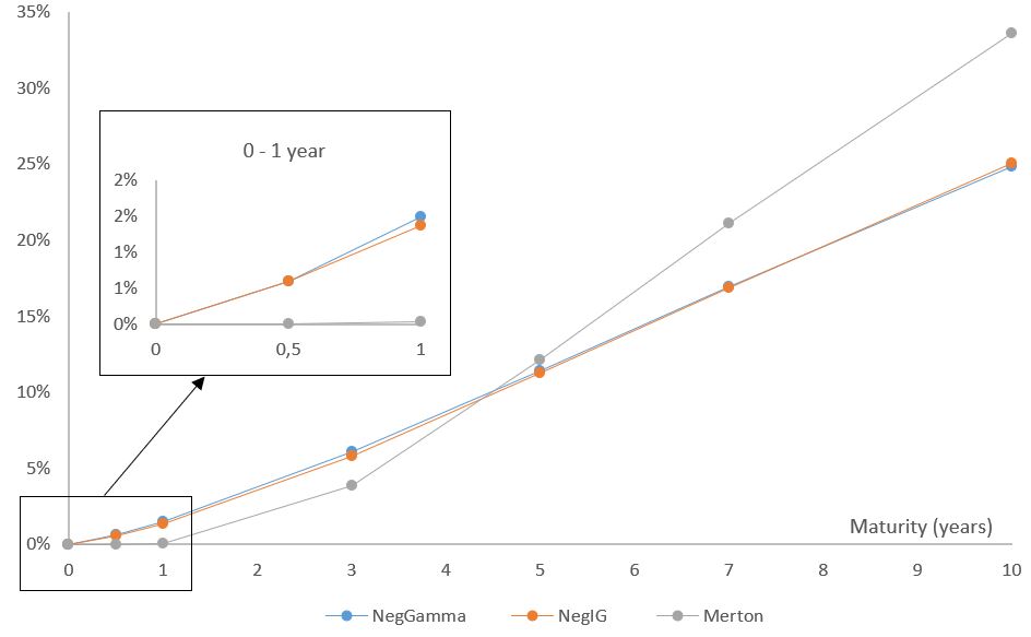
In Fig. 1, we plot the term structure of the default probabilities for the GET FP issuer (0 to 10 years), in the NegGamma, NegIG and Merton models. We can recognize the characteristic shape of the Merton default probabilities: short term probabilities are very low, with a sudden increase and an inflection around 5 years and a flattening for longer horizons (which is a direct consequence of the shape of the normal cumulative distribution function N(.)). On the contrary, NegGamma and NegIG default probabilities display a more regular structure across maturities, and a clearly visible risk redistribution towards shorter time horizons, while Merton default probabilities are null for T 1, and reach 35% on the 10 years horizon, which is completely incoherent with the historical default rates of this category.
3.3.2 Actual (real-world) default probabilities
In this subsection, we discuss actual (real world) default probabilities (25). Model parameters are calibrated using algorithm 1, while the actual drift is calibrated for each issuer thanks to formula (35), in both cases using market data on a 2 year period. This is to avoid enormous drifts such as that can arise on a 1 year period (notably 2020) and lead to absurdly small or big default probabilities. In table 4, we compare the actual default probabilities obtained for the set of issuers (see details in appendix B) with our NegGamma and NegIG models to the one obtained via the classical Merton model, for two distinct horizons (1 year and 5 years). We also compare with historical default rates of the investment grade and speculative categories displayed in table 3.
| Category | 1 year default rate | 5 years default rate | 10 years default rate | |||
|---|---|---|---|---|---|---|
| 2010-2019 | 2009 | 2010-2015 | 2009 | 2000-2008 | 2009 | |
| Investment Grade | 0.01% | 0.33% | 0.17% | 0.63% | 2.15% | 0.92% |
| Speculative | 2.53% | 9.95% | 10.01% | 16.47% | 21.3% | 20.74% |
| All ratings | 1.19% | 4.19% | 4.61% | 6.99% | 9.43% | 8.88% |
| Rating | Category | NegGamma | NegIG | Merton | ||||
| = 1 y. | =5 y. | = 1 y. | =5 y. | =1 y. | =5 y. | |||
| SAP GY | A | Inv | 0.01% | 0.04% | 0.01% | 0.04% | 0.00% | 0.00% |
| MRK GY | A | Inv | 0.02% | 0.09% | 0.03% | 0.09% | 0.00% | 0.00% |
| AI FP | A- | Inv | 0.02% | 0.05% | 0.02% | 0.05% | 0.00% | 0.00% |
| SU FP | A- | Inv | 0.03% | 0.06% | 0.03% | 0.06% | 0.00% | 0.00% |
| CRH LN | BBB+ | Inv | 0.37% | 1.56% | 0.35% | 1.50% | 0.00% | 0.22% |
| SRG IM | BBB+ | Inv | 0.83% | 3.39% | 0.74% | 3.18% | 0.00% | 0.82% |
| DAI GY | BBB+ | Inv | 2.11% | 13.72% | 1.92% | 13.50% | 0.10% | 15.76% |
| VIE FP | BBB | Inv | 1.39% | 7.52% | 1.25% | 7.24% | 0.01% | 5.16% |
| AMP IM | BB+ | Spec | 0.12% | 0.16% | 0.12% | 0.16% | 0.00% | 0.00% |
| FR FP | BB+ | Spec | 1.93% | 11.07% | 1.79% | 10.91% | 0.12% | 11.25% |
| EO FP | BB | Spec | 2.72% | 20.02% | 2.57% | 19.98% | 0.52% | 22.42% |
| GET FP | BB- | Spec | 0.68% | 4.00% | 0.63% | 3.83% | 0.00% | 1.64% |
| LHA GY | BB- | Spec | 9.45% | 81.73% | 9.13% | 81.93% | 8.56% | 82.53% |
| PIA IM | B+ | Spec | 0.53% | 1.71% | 0.41% | 1.66% | 0.00% | 0.46% |
| CO FP | B | Spec | 13.82% | 88.99% | 13.57% | 88.82% | 14.67% | 87.14% |
We can observe that:
- -
Like in the risk-neutral case, actual default probabilities are significantly higher in the NegGamma and NegIG models than in the Merton model;
- -
On the speculative segment, 1 year actual default probabilities are typically around 1-3% in the NegIG and NegGamma models (except for the very indebted issuers already discussed), which provides a very good agreement with the 2010-2019 average for 1 year default rates in this category (2.53%).
- -
Still on the speculative segment but for longer (5Y) maturities, actual default probabilities of all models tend to converge to similar values, highlighting the predominant role of the drift for longer horizons, except for issuers with the best signature (such as AMP or PIA) where NegGamma or NegIG default probabilities remain higher than the Merton ones, and closer to 5Y historical default rates.
- -
It is interesting to note that, for the best rated issuers retained in our study, 1 and 5 years actual default probabilities provide a remarkably good fit to historical default rates, while Merton probabilities remain equal to for all maturities. For the other issuers of the investment grade segment, NegGamma and NegIG default probabilities appear to slightly overestimate short term historical default rates; we may note, however, that these probabilities can easily be diminished by usual data re-processings of the equity or debt values for such issuers. For instance, an important part of a firm’s debt can be concentrated by one of its financial captive, as frequently the case in the automobile industry (DAI GY); it is therefore common to lower the face value of the total debt by the captive debt amount. Other issuers, for instance operating in the energy sector (like VIE FP), require expensive equipment with long term financing, and in that case a common practice is to integrate operational cashflows to the market capitalization () of the firm when evaluating its default risk.
3.4 Convergence analysis
In table 5, we indicate the minimal, maximal and average number of steps needed to reach a precision of when applying algorithm 1 to the data set of table 8, as well as the corresponding elapsed time (in seconds). The calculations are made on a personal computer with Intel(R) Core(TM) i5-8265U CPU @1.60GHz. Clearly, one can observe that the number of steps, although increasing with maturity, remains very small and that elapsed time is around or even less than a second.
| NegGamma | NegIG | Merton | |||||||
| Number of steps | Min | Max | Av. | Min | Max | Av. | Min | Max | Av. |
| 1Y | 3 | 7 | 4.48 | 2 | 6 | 3.71 | 2 | 7 | 4.05 |
| 5Y | 3 | 11 | 5.95 | 3 | 8 | 4.76 | 3 | 13 | 6.61 |
| 10Y | 3 | 13 | 6.90 | 3 | 10 | 5.38 | 3 | 17 | 8.24 |
| 15Y | 4 | 15 | 7.43 | 3 | 11 | 6.00 | 4 | 18 | 8.86 |
| Elapsed time (in sec) | Min | Max | Av. | Min | Max | Av. | Min | Max | Av. |
| 1Y | 0.48 | 1.25 | 0.74 | 0.16 | 0.53 | 0.32 | 0.08 | 0.31 | 0.16 |
| 5Y | 0.57 | 2.23 | 1.11 | 0.25 | 0.71 | 0.42 | 0.11 | 0.55 | 0.27 |
| 10Y | 0.56 | 2.65 | 1.33 | 0.29 | 0.88 | 0.49 | 0.12 | 0.61 | 0.31 |
| 15Y | 0.75 | 3.30 | 1.45 | 0.33 | 1.12 | 0.58 | 0.15 | 0.63 | 0.33 |
4 A symmetric model
Let us now consider the case where the stochastic process in (4) is a symmetric Lévy process, that is, a process with equally probable downward and upward jumps. We will consider a Variance Gamma (VG) process, which, for simplicity, will be assumed to be symmetric. VG processes have already been introduced in credit risk models in Foriani & al. 2006; Fiorani & al. 2010, but using a calibration from CDS indices (Markit CDX.NA.HY and CDX.NA.IG). Again, we adopt a different approach, by taking advantage of recently derived pricing formulas for the European call to perform algorithm 1 on each firm’s own equity, and deduce its default probability.
4.1 The symmetric Variance Gamma (symVG) credit risk model
The Variance Gamma (VG) process, which has been popularized in financial modelling in Madan et al. 1998, can be defined by a time changed drifted Brownian motion:
| (66) |
where is a Gamma process of mean and variance (note that this parametrization is equivalent to the rate/shape parametrization of subsection 3.1, for and ). is the scale parameter and the asymmetry, or sknewness parameter; in the case the distribution of the VG process is symmetric around the origin (this model was introduced earlier, in Madan & Seneta 1990). The definition (66) shows that the VG process is actually a so-called normal mean mixture (Barndorff-Nielsen & al. 1982), where the mixing distribution is given by the Gamma distribution and materializes the passage of the business time, jumps in the process materializing periods of intense trading activity. When grows high then jumps are more frequent and the business time admits staircase-like realizations; on the contrary, the configuration corresponds to a linear passage of time.
The Lévy measure of the VG process is known to be
| (67) |
which shows that the VG process is a particular case of a CGMY process (Carr & al. 2002). As the measure (67) is defined on the whole real axis, realizations of the VG process feature both upward and downward jumps; while downward jumps still materialize a brutal drop in a firm’s assets, we may think of upward jumps as cash injections from governmental institutions or central banks in order to help recapizalizing severely indebted issuers. Let us also remark that when then the Lévy measure is symmetric around 0 (and in that case positive and negative jumps occur with equal probability). The Lévy symbol can be computed from (67) and the Lévy-Khintchine formula (7), resulting in
| (68) |
from which we easily deduce the cumulant generating function as well as the first cumulants and central moments:
| (69) |
If we assume , the tails are symmetric and the skewness is equal to and the kurtosis becomes
| (70) |
highlighting the role of as the measure of excess kurtosis of the distribution.
4.2 Default metrics
When the VG process is symmetric, its density is known to be
| (71) |
and, taking in (68), we easily obtain the convexity adjustment
| (72) |
From definition 1, the distance to default in the symVG model is therefore
| (73) |
Remark 4.
In the low kurtosis regime , Taylor expanding (72) yields , thus recovering the Gaussian adjustment; in other words, the symVG model recovers the Merton model in its low kurtosis limit.
The cumulative distribution function of the Variance Gamma distribution is not known in exact form but easily accessible from any programming language. For instance in R one can use the CDF function applied to the Variance Gamma density (denoted by "dvg" in the Variance Gamma package), and the default probability in the symVG model can be written formally as:
| (74) |
4.3 Equity value
An exact formula for the price of the European call under the VG process has been established in Madan et al. 1998, but it involves complicated products of Bessel and hypergeometric functions; in practice, Fourier techniques are favored (Lewis 2001), notably because of the relative simplicity of the characteristic exponent (68). This technology, however, is not adapted to the implementation of algorithm 1 because if would call for solving an equation involving an integral in the Fourier space. Instead, we propose to use a recently derived pricing formula for the European call in the symmetric VG model, which takes the form of quickly convergent series of powers of the log forward moneyness (or, in the context of default modelling, of the distance to default). To that extent, let us introduce the notations
| (75) |
and assume . For , let us also define the quantity
| (76) |
Proposition 4.1.
The equity value of a firm in the symVG credit risk model can be written as:
- -
If ,
(77) - -
If ,
(78) - -
If ,
(79)
Proof.
See Aguilar 2020. ∎
4.4 Parameter calibration and default probabilities
The calibration procedure is, like for one-sided models, based on algorithm 1 and proposition 4.1. Note that, typically, it is sufficient to truncate the series at to get a precision of on equity prices, and that machine precision is reached between 15 and 20 iterations (see an example on the issuer GET FP in table 7); convergence can be slightly slower if the ratio becomes very small, but remains very efficient in all cases (and is particularly accelerated for short maturities). We also refer to Aguilar & Kirkby 2021 for a precise discussion and comparison of the pricing formula in proposition 4.1 with state of the art numerical pricing techniques such as Fast Fourier Transform and their recent refinements (COS, PROJ etc.).
Given the moments (69) for , we need to consider the function
| (80) |
whose inversion is immediate. Calibration results and default probabilities are displayed in table 6; we only estimate risk-neutral default probabilities; estimation of real-world is straightforward using the same technique as for one-sided models described in subsection 2.4.2.
| Issuer | Calibrated parameters | Default probabilities | ||||
|---|---|---|---|---|---|---|
| (in MM) | SymVG | Merton | NegGamma | |||
| SAP GY | 0.2873 | 2.2526 | 180 904 | 0.00 % | 0.00% | 0.01% |
| AI FP | 0.2340 | 3.5774 | 78 923 | 0.03 % | 0.00% | 0.08% |
| SU FP | 0.3246 | 3.9171 | 71 472.2 | 0.07% | 0.00% | 0.14% |
| CRH LN | 0.3038 | 2.9005 | 33 948.2 | 0.57% | 0.01% | 1.10% |
| SRG IM | 0.1942 | 6.3719 | 29 556.2 | 0.91% | 0.02% | 1.73% |
| DAI GY | 0.1026 | 3.5876 | 213800 | 1.61% | 0.55% | 3.26% |
| VIE FP | 0.1618 | 4.4099 | 27 281.3 | 1.42% | 0.21% | 2.62% |
| AMP IM | 0.3598 | 4.809 | 8 627.48 | 0.26% | 0.00% | 0.50% |
| FR FP | 0.2741 | 3.1256 | 11 931.5 | 1.02% | 0.62% | 3.12% |
| EO FP | 0.2754 | 1.7378 | 10 010.3 | 1.69% | 0.65% | 3.06% |
| GET FP | 0.2402 | 3.2453 | 11 666.7 | 0.79% | 0.03% | 1.50% |
| LHA GY | 0.2092 | 2.5558 | 14 700 | 4.40% | 5.09% | 7.29% |
| PIA IM | 0.2513 | 1.8526 | 1 494.92 | 0.57% | 0.02% | 1.08% |
| CO FP | 0.0713 | 2.6652 | 16 427.4 | 3.30% | 2.48% | 5.62% |
It is interesting to note that 1 year symVG default probabilities are all comprised between 1 year Merton and 1 year NegGamma default probabilities (except for LHA GY). The fact that symVG probabilities are lower than the probabilities computed in a one-sided model (the NegGamma model) is no surprise, since the symVG model features also positive jumps (i.e. sudden raises in asset prices), which can diminish the probability for to be lower than ; the symVG model is therefore more tempered than the NegGamma model, but its default probabilities remain very significantly higher than in the Merton model, except for top quality issuers.
5 Concluding remarks
In this study, we have generalized the notions of distance to default and default probabilities to the class of pure jump structural models, and studied two sub-classes: one-sided models (NegGamma, NegIG) and symmetric models (symVG). One-sided models are particularly tractable, thanks to the closed formulas for the equity value that we have established (propositions 3.1 and 3.2). Such closed formulas make the calibration algorithm easy to implement.
One-sided models produce higher short term default probabilities (both risk-neutral and real world) than the Merton model. In particular, these probabilities typically lie between 0.5% and 3% for speculative issuers, which is close to the historical 1 year default rate of this category. On the investment grade segment, high quality issuers (with a ranking higher or equal to A) have a small default probability (0.01-0.15%) which is coherent with the quality of their signature; the figures, however, remain clearly higher than the Merton ones.
In double-sided models (symVG), the presence of upward jumps moderates the probability for to be lower than , and therefore default probabilities are lower than NegGamma and NegIG default probabilities, while remaining higher than the Merton ones. The model is, consequently, well suited to investment grade issuers for longer horizons, but as the equity value is only accessible via truncated series expansions, the calibration algorithm takes more time to converge.
Future work should include the consideration of other dynamics for asset prices, such as a double-sided process with asymmetric distribution of jumps; recent pricing formulas established for instance in the case of an asymmetric NIG process could be used for computing the equity value, but their series nature will call for several optimization in the calibration algorithm to maintain a satisfactory level of performance.
Acknowledgments
We thank Alexander Lipton for his interest in this work and his many valuable comments. We also thank two anonymous reviewers whose detailed reports greatly helped us improve the quality of the manuscript.
References
- Aguilar (2020) Aguilar, J.-Ph., Some pricing tools for the Variance Gamma model, International Journal of Theoretical and Applied Finance 23(4), 2050025 (2020)
- Aguilar & Kirkby (2021) Aguilar, J.-Ph. and Kirkby, J. L., Closed-form option pricing for exponential Lévy models: a residue approach, Available at SSRN: https://ssrn.com/abstract=3823337 (2021). Accessed 31st July 2021.
- Abramowitz & Stegun (1972) Abramowitz, M. and Stegun, I., Handbook of Mathematical Functions, Dover Publications, Mineola, NY (1972)
- Bai et al. (2020) Bai, J., Goldstein, R. and Yang, F., Is the credit spread puzzle a myth?, Journal of Financial Economics 1327(2), 297-319 (2020)
- Barndorff-Nielsen & al. (1982) Barndorff-Nielsen, O., Kent, J. and Sørensen, M., Normal Variance-Mean Mixtures and z Distributions, International Statistical Review 50(2), 145-159 (1982)
- Barndorff-Nielsen (1995) Barndorff-Nielsen, O., Normal inverse Gaussian distributions and the modeling of stock returns, Research report no 300, Department of Theoretical Statistics, Aarhus University (1995)
- Barndorff-Nielsen (1997) Barndorff-Nielsen, O., Normal inverse Gaussian distributions and stochastic volatility modelling, Scandinavian Journal of Statistics 24(1), 1-133 (1997)
- Bertoin (1996) Bertoin, J., Lévy Processes, Cambridge University Press, Cambridge, New York, Melbourne (1996)
- Bingham (1973) Bingham, N. H., Maxima of sums of random variables and suprema of stable processes, Zeitschrift für Wahrscheinlichkeitstheorie und Verwandte Gebiete, Vol. 26 Issue 4, Springer, Berlin, Heidelberg (1973)
- Black & Scholes (1973) Black, F. and Scholes, M., The Pricing of Options and Corporate Liabilities, Journal of Political Economy 81(3), 637-654 (1973)
- Black & Cox (1976) Black, F. and Cox, J., Valuing Corporate Securities: Some Effects of Bond Indenture Provisions, Journal of Finance 31(2), 352-367 (1976)
- Carr & al. (2002) Carr, P., Geman H., Madan D. and Yor, M., The fine structure of asset returns: An empirical investigation, Journal of Business 75(2), 305-332 (2002)
- D’Amato & Remolona (2003) D’Amato, J. and Remolona, E., The credit spread puzzle, BIS Quarterly Review (2003)
- Delianedis & Geske (2003) Delianedis, G. and Geske, R.L., Credit Risk and Risk Neutral Default Probabilities: Information About Rating Migrations and Defaults, available at SSRN: https://ssrn.com/abstract=424301 (2003). Accessed 31st July 2021.
- Demchuk & Gibson (2009) Demchuk, A. and Gibson, R. Stock Market Performance and the Term Structure of Credit Spreads, Journal of Financial and Quantitative Analysis 41(4), 863-887 (2009)
- Duan & al. (2004) Duan, J.-C., Gauthier, G. and Simonato, J.-G., On the equivalence of the kmv and maximum likelihood methods for structural credit risk models, Working paper (2004). Available at https://www.fdic.gov/analysis/cfr/2005/apr/jcduan-ggauthier-jsimonato.pdf (accessed 31st July 2021).
- Duffie & Singleton (1999) Duffie, D. and Singleton, K.J., Modeling Term Structures of Defaultable Bonds, The Review of Financial Studies 12(4), 687-720 (1999)
- Duffie & Singleton (2012) Duffie, D. and Singleton, K.J., Credit risk: pricing, measurement, and management, Princeton university press, Princeton (NJ) (2012)
- Duyvesteyn & Martens (2015) Duyvesteyn, J. and Martins, M., Forecasting Sovereign Default Risk with Merton’s Model, The Journal of Fixed Income 25 (2), 58-71 (2015)
- Eom & al. (2004) Eom, Y.H., Helwege, J. and Huang, J.-Z., Structural Models of Corporate Bond Pricing: An Empirical Analysis, The Review of Financial Studies 17(2), 499-544 (2004)
- Ericsson & Reneby (2002) Ericsson, J. and Reneby, J., A Note on Contingent Claims Pricing with Non-Traded Assets, SSE/EFI Working Paper Series in Economics and Finance No 314 (2002)
- Foriani & al. (2006) Fiorani, F. and Luciano, E., Credit Risk in Pure Jump Structural Models, ICER Working Paper No. 6/2006, Available at SSRN: https://ssrn.com/abstract=932047 (2006). Accessed 31st July 2021.
- Fiorani & al. (2010) Fiorani, F., Luciano, E. and Semeraro, P., Single and Joint Default in a Structural Model with Purely Discontinuous Asset Prices, Quantitative Finance 10(3), 249-263 (2010)
- Geske (1977) Geske, R., The valuation of corporate liabilities as compound options, Journal of Financial and Quantitative Analysis 12, 541-552 (1977)
- Glasser (1983) Glasser, M.L., A Remarkable Property of Definite Integrals, Mathematics of Computation 40, 561-563 (1983)
- Gray & al. (2007) Gray, D., Merton, R. and Bodie, Z., Contingent claims approach to measuring and managing sovereign credit risk, Journal of Investment Management 5(4), 5-28 (2007)
- Gregory (2015) Gregory, J., The xVA Challenge: Counterparty Credit Risk, Funding, Collateral, and Capital, John Wiley & Sons, Hoboken, NJ (2015)
- Hilberink & Rogers (2002) Hilberink, B. and Rogers, L. C. G., Optimal capital structure and endogenous default, Finance and Stochastics 6, 237-263 (2002)
- Jones & al. (1984) Jones, E.P., Mason, S.P. and Rosenfeld, E., Contingent claims analysis of corporate capital structures: An empirical investigation, Journal of Finance 39, 611-627 (1984)
- Huang & al. (2019) Huang, J.-Z., Nozawa, Y. and Shi, Z., The Global Credit Spread Puzzle, PBCSF-NIFR Research Paper, Available at SSRN: https://ssrn.com/abstract=3453959 or http://dx.doi.org/10.2139/ssrn.3453959 (2019)
- Kou (2002) Kou, S., A Jump-Diffusion Model for Option Pricing, Management Science 48(8), 1086-1101 (2002)
- Küchler & Tappe (2008) Küchler U. and Tappe, S., Bilateral gamma distributions and processes in financial mathematics, Stochastic Processes and their Applications 118(2), 261-283 (2008)
- Le Courtois & Quittard-Pinon (2006) Le Courtois, O. and Quittard-Pinon, F., Risk-neutral and actual default probabilities with an endogenous bankruptcy jump-diffusion model, Asia-Pacific Financial Markets 13, 11-39 (2006)
- Leland & Toft (1996) Leland, H. and Toft, K. B., Optimal Capital Structure, Endogenous Bankruptcy, and the Term Structure of Credit Spreads, The Journal of Finance 51(3), 987-1019 (1996)
- Lewis (2001) Lewis, A.L., A simple option formula for general jump-diffusion and other exponential Lévy processes, Available at SSRN: https://ssrn.com/abstract=282110 (2001)
- Lipton (2002) Lipton, A., Assets with jumps, Risk Magazine 15(9), 143-153 (2002)
- Lipton & Sepp (2009) Lipton, A. and Sepp, A., Credit value adjustment for credit default swaps via the structural default model, The Journal of Credit Risk 5(2), 123-146 (2009)
- Lipton & Rennie (2013) Lipton, A. and Rennie, A., Eds., The Oxford Handbook of Credit Derivatives, Oxford University Press (2013)
- Longstaff & Schwartz (1995) Longstaff, F. and Schwartz, E., A Simple Approach to Valuing Risky Fixed and Floating Rate Debt, Journal of Finance 50(3), 789-819 (1995)
- Luciano (2009) Luciano, E., Business Time and New Credit Risk Models, Convegno Economia e Incertezza, Trieste (2009)
- Lyden & Saraniti (2000) Lyden, S. and Saraniti, D., An Empirical Examination of the Classical Theory of Corporate Security Valuation, http://dx.doi.org/10.2139/ssrn.271719 (2000)
- Ma & Xu (2016) Ma, Y. and Xu, W., Structural credit risk modelling with Hawkes jump diffusion processes, Journal of Computational and Applied Mathematics 303, 69-80 (2016)
- Madan & Seneta (1990) Madan, D. and Seneta, E., The Variance Gamma (V.G.) Model for Share Market Returns, The Journal of Business 63(4), 511-524 (1990)
- Madan et al. (1998) Madan, D., Carr, P., Chang, E., The Variance Gamma Process and Option Pricing, European Finance Review 2, 79-105 (1998)
- Madan & Schoutens (2008) Madan, D. and Schoutens, W., Break on Through to the Single Side, Working Paper, Katholieke Universiteit Leuven (2008)
- Marfè (2012) Marfè, R., A Multivariate Pure-Jump Model with Multi-Factorial Dependence Structure, International Journal of Theoretical and Applied Finance 15(4), 1250028 (2012)
- Merton (1974) Merton, R., On the pricing of corporate debt: the risk structure of interest rates, Journal of Finance 29(2), 449-470 (1974)
- Pasricha & al. (2021) Pasricha, P., Lu, X. and Zhu, S.-P., A note on the calculation of default probabilities in “Structural credit risk modeling with Hawkes jump–diffusion processes”, Journal of Computational and Applied Mathematics 381, 113037 (2021)
- Kraemer (2020) Kraemer, N.W, Default, Transition and Recovery: The Global Recession is Likely to Push the US Default Rate to 10%, S&P Global ratings research note (2020), available at https://www.spglobal.com/ratings/en/research/articles/200320-default-transition-and-recovery-the-global-recession-is-likely-to-push-the-u-s-default-rate-to-10-11396924 (accessed 31 July 2021)
- Kraemer & al. (2020) Kraemer, N.W, Fernandes, L., Pranshu, S. and Richhariya, N.M., 2019 Annual Global Corporate Default And Rating Transition Study, S&P Global ratings research note (2020), available at https://www.spglobal.com/ratings/en/research/articles/200429-default-transition-and-recovery-2019-annual-global-corporate-default-and-rating-transition-study-11444862 (accessed 31 July 2021)
- Schoutens (2003) Schoutens, W., Lévy processes in finance: pricing financial derivatives, John Wiley & Sons, Hoboken, NJ (2003)
- Shuster (1968) Shuster, J., On the Inverse Gaussian distribution function, Journal of the American Statistical Association 63, 1514-1516 (1968)
- Stein (2016) Stein, H.J., Fixing risk neutral risk measures, International Journal of Theoretical and Applied Finance 19(3), 1650021 (2016)
- Vassalou and Xing (2004) Vassalou, M. and Xing, Y., Default Risk in Equity Returns Journal of Finance 59(2), 831-868 (2004)
- Zhou (1997) Zhou, C., A jump-diffusion approach to modeling credit risk and valuing defaultable securities, Finance and Economics Discussion Series 1997-15, Board of Governors of the Federal Reserve System (1997)
Appendix A Notations used in the paper
Special functions
Standard normal cumulative distribution function:
| (81) |
Lower incomplete Gamma function:
| (82) |
Upper incomplete Gamma function:
| (83) |
Bessel function of the second kind (MacDonald function):
| (84) |
Shuster’s integrals 22 2 This is a consequence of the Cauchy - Schlömilch substitution (85) which is itself a consequence of the more general Glasser’s master theorem (Glasser 1983). (Shuster 1968):
| (86) |
Model notations
Characteristic function and Lévy symbol:
| (87) |
Moment generating function (double-sided Laplace transform):
| (88) |
Cumulant generating function:
| (89) |
cumulant:
| (90) |
Standardized central moments of a time series :
| (91) |
| (92) |
Subset of standardized central moments of order :
| (93) |
Cumulative distribution function (process with density ):
| (94) |
Martingale adjustment:
| (95) |
Risk-neutral and Actual distance to default:
| (96) |
Risk-neutral and Actual default probability:
| (97) |
Appendix B Data set
To test the models, we have chosen a set of issuers from various European markets, which are representative of several industrial sectors and S&P rating categories. In table 8 we provide details on the issuers and the debt level chosen in our study.
| Ticker | Name | Industry group | Total debt (in MM) | Category |
|---|---|---|---|---|
| SAP GY | SAP SE | Software | 16 196 | Investment |
| MRK GY | Merck KGAA | Pharmaceuticals | 14 180 | Investment |
| AI FP | Air Liquide SA | Chemicals | 14 730 | Investment |
| SU FP | Schneider Electric SE | Electrical Components | 8 473 | Investment |
| CRH LN | CRH PLC | Building materials | 10 525 | Investment |
| SRG IM | Snam SPA | Gas | 14 774 | Investment |
| DAI GY | Daimler AG | Auto manufacturers | 161 780 | Investment |
| VIE FP | Veolia Environment | Water | 16 996 | Investment |
| AMP IP | Amplifon SPA | Pharmaceuticals | 1 339 | Speculative |
| FR FP | Valeo SA | Auto parts & Equipment | 4 879 | Speculative |
| EO FP | Faurecia | Auto parts & Equipment | 4 838 | Speculative |
| GET FP | Getlink SE | Transportation | 4 998 | Speculative |
| LHA GY | Deutsche Lufthansa | Airlines | 10 106 | Speculative |
| PIA IM | Piaggio | Motorcycles | 609 | Speculative |
| CO FP | Casino | Foods | 14 308 | Speculative |
Appendix C Stability of the parameters
In figure 2, we plot the evolution of calibrated parameters in function of debt maturity , for 2 representative issuers and the NegGamma, NegIG and Merton models. The parameters do not significantly evolve with ; this is perfectly consistent with the fact that the time series of the log-returns of used for the calibration is not affected by the choice made for the debt maturity .


Appendix D Code
The R code written to implement algorithm 1 on the whole data set displayed in table 8 and to estimate default probabilities is publicly available at https://github.com/Voxinat/CreditRiskModels.