Using Echo State Networks to Approximate Value Functions for ControlJournal: Neural Networks
Abstract
An Echo State Network (ESN) is a type of single-layer recurrent neural network with randomly-chosen internal weights and a trainable output layer. We prove under mild conditions that a sufficiently large Echo State Network can approximate the value function of a broad class of stochastic and deterministic control problems. Such control problems are generally non-Markovian.
We describe how the ESN can form the basis for novel and computationally efficient reinforcement learning algorithms in a non-Markovian framework. We demonstrate this theory with two examples. In the first, we use an ESN to solve a deterministic, partially observed, control problem which is a simple game we call ‘Bee World’. In the second example, we consider a stochastic control problem inspired by a market making problem in mathematical finance. In both cases we can compare the dynamics of the algorithms with analytic solutions to show that even after only a single reinforcement policy iteration the algorithms arrive at a good policy.
Keywords:
Liquid State Machines , Reservoir Computing , Stochastic Optimal Control , Mathematical Finance , Reinforcement LearningPACS
0000 , 1111MSC
0000 , 11111 Introduction
An Echo State Network (ESN) is a special type of single-layer recurrent neural network introduced at the turn of the millennium by [1] and [2] to study time series. Training is fast because the training step involves only the selection of weights in the output layer rather than updating the internal weights in the recurrent layer. Furthermore, the simple formulation of ESNs renders them amenable to mathematical analysis. Given a time series (where is the discrete time index) of -dimensional data points, an ESN is set up as follows. We randomly generate a reservoir matrix , a input matrix and a bias vector . Then we iteratively generate a sequence of -dimensional reservoir state vectors according to
where is the rectified linear unit (ReLU) activation function applied component-wise to the -dimensional vector . Observe that the th reservoir state depends on all past data-points and therefore captures non-Markovian temporal correlations in the data. If the 2-norm of the reservoir matrix satisfies then as tends to infinity, the influence on the reservoir state of the data points in the distant past becomes arbitrarily small. This is called the fading memory property and is closely related to the echo state property (ESP) introduced in the context of ESNs by [1]. The ESP is the statement that the sequence of reservoir states is, for a given input data sequence , uniquely determined. We can interpret the reservoir state vectors as the latent vectors which encode the infinite past observations in lower dimensional form.
When an ESN has the ESP, it can be applied to a class of supervised learning problems where we have a time series of dimensional data points , called targets, that depend on all previous input time series data and we seek to learn the relationship between the sequence of past states and the target for each . We can train an ESN to solve this problem by finding the matrix that minimises
where is the number of labelled data points, and is the Tikhonov regularisation (a.k.a. ridge regression) parameter. Throughout this paper, denotes the matrix 2-norm, vector 2-norm or absolute value, depending on whether the input is a matrix, vector, or scalar, respectively.
This minimisation problem can be solved using regularised linear least squares regression, and hence we can both obtain quickly, and guarantee that is the global optimum. This compares extremely favourably with training a (deep) neural network with stochastic gradient descent and backpropagation which takes considerably longer, and may not converge to the global optimum [3].
Despite the training procedure being entirely linear, ESNs are universal approximators, and can therefore model arbitrarily complex relationships between the sequence of past data points and the targets. This is made formal in a recent result by [4] that we review here and then build on. We emphasise that not only are ESNs theoretically very promising, they have performed remarkably well in practice on problems ranging from seizure detection, to robot control, handwriting recognition, and financial forecasting, where ESNs have won competitions [5], [6], [7], [8]. Impressively, ESNs outperformed RNNs and LSTMs at a chaotic time series prediction task by a factor of over 2400 [9]. ESNs have also proved themselves competitive in various tasks in reinforcement learning [10] and control [11].
Even in cases where practitioners prefer to use other recurrent neural networks (RNNs), such as Long Short Term Memory networks (LSTMs), the rigorous theory of ESNs should prove useful in architecture design. In [12], it is shown that different deep neural network architectures can be ranked by randomly initialising the internal weights and training only the outer weights by linear regression. Once the best performing architecture (with random internal weights) has been identified, the authors then train the internal weights of the highest ranking architecture. This is much faster than training the internal weights (a nonlinear problem) for every architecture. The ranking of architectures with random internal weights closely approximates the ranking of architectures with optimised internal weights. From our point of view, the authors are essentially approximating fully trained networks with (non-recurrent) ESNs.
In a sequence of papers, [13], [14], and [4] recently analysed ESNs in the context of nonlinear filters and functionals. Roughly speaking, a filter is a map from a bi-infinite sequence of real vectors to another bi-infinite sequence of real vectors , and a functional maps a bi-infinite sequence of real vectors to a single real vector or number. We can view an ESN as a filter that maps an input sequence to a reservoir sequence , or a funtional that maps to the lone reservoir state . The theory of filters and functionals is therefore a natural theoretical setting for ESNs. Within this theory, this paper presents three novel results.
Our first result assumes that we have a time series of data and a set of targets that depend on all previous data points via a functional which sends infinite sequences of data points to targets. We then have a supervised learning problem of finding the relationship between the data and targets. In the special case that , this problem is time series forecasting. Our first novel result states that if we have sufficiently many data points , drawn from a stationary, ergodic, and bounded process , which need not be Markovian, and we obtain using regularised linear least squares, then a sufficiently large ESN will approximate, as closely as required, the functional sending inputs to the targets .
This result has applications in the statistical inference of dynamical systems, which was recently reviewed by [15]. This area of research is especially focused on statistical inference (i.e learning) of stationary ergodic processes. Furthermore, we can use this result in the context of reinforcement learning (RL) and optimal control. We envisage an agent operating under a given policy in the parlance of reinforcement learning or control in the parlance of control theory that generates a sequence of (reward, action, observation) triples . Then the functional that maps previous (reward, action, observation) triples to rewards models the reward functional arbitrarily well. The set up does not assume the RL problem is Markovian, and allows for a continuous state space.
Our second novel result generalises the first, and encompasses the case where the functional is the value functional of a stochastic control process, or Partially Observed Markov Decision Process (POMDP). By training an ESN to approximate the value functional, we establish a stepping stone toward developing an offline reinforcement learning algorithm supported by an ESN that can solve a large class of control problems. Moreover, since ESNs are recurrent, they can be used for non-Markovian problems, where a reinforcement learning agent must exploit its memory of past observations, actions and rewards. Our third result is presented in the context of building an online reinforcement algorithm that can, under certain conditions, determine the optimal value function for a given policy.
These results are part of a general push to take machine learning ideas typically applied to (partially observed) Markov processes and generalising them to hold on stationary ergodic processes. We can see for example [16] consider to clustering problems typically defined Markov processes applied to stationary ergodic processes.
We demonstrate some of these theoretical results numerically on two examples. The first is a deterministic game which we call ‘Bee World’. The goal of the game for the bee is to navigate a time varying distribution of nectar in order to maximise the total future discounted value of the nectar acquired over all future time. The optimal trajectory can be found explicitly via the calculus of variations but the constraint that the bee has a maximum speed of flight leads to unexpectedly complicated solution paths; it therefore provides a straightforward but not entirely trivial control problem. Since the bee does not have access to the entire state space, and only observes the nectar it collects at each moment in time, the problem is therefore a partially observed Markov Decision Process which requires memory of the past to solve. We demonstrate how a simple and easily-configurable reinforcement learning algorithm supported by an ESN can learn to play Bee World with respectable skill.
The second numerical example is inspired by a market making problem in mathematical finance. The mathematical formulation of this problem reduces to a seeking to control a one dimensional Brownian motion so that it stays near the origin. The cost of straying from the origin is quadratic in the distance from the origin, and the cost of applying a push toward the origin is quadratic in the strength of the push. The market maker must therefore balance the cost of applying the control against the cost of allowing the motion to drift too far from the origin. We briefly discuss the financial motivation for this problem, then solve it analytically in continuous and discrete time. The set up most commonly seen in the literature is continuous time, but only in discrete time is the problem suitable for an ESN. We then compare the optimal discrete time solution to a solution learned by a reinforcement learning agent supported by an ESN.
Finally, we note that our approach to the Market making problem is loosely related to the recent paper by [11] who introduce QuaSiModO: Quantization-Simulation-Modeling-Optimization. These authors analyse the interplay between the following four aspects:
- 1.
Quantising the action space .
- 2.
Simulating a system under a given control/policy.
- 3.
Modelling the full system given a partial/full observation of the state space.
- 4.
Optimising the control/policy.
The structure of the remainder of the paper closely follows the summary of results presented above. In section 2 we set up the mathematical formalism for ESNs that we wish then to approximate. Section 3 introduces our novel theoretical results, while sections 4 and 5 respectively present applications to the deterministic (‘Bee World’), and then the stochastic (‘market maker’) optimal control problems. We conclude in section 6.
2 Background
In this section, we introduce the theory and notation of nonlinear filters (in relation to ESNs) developed by [13], [14], and [4]. First, we denote by the set of maps with domain and codomain . This is the set of bi-infinite –valued real sequences.
A filter is a map . A filter is called causal if inputs from the past and present contribute to but states in the future do not. More formally is casual if that satisfy it follows that . We define the time shift filter by which we interpret as the map that steps forward one unit of time. A filter is called time invariant if commutes with the time shift operator . If is causal and time invariant filter then we call a causal time invariant (CTI) filter.
A functional is a map . In [14] it is shown that there is a bijection between the space of CTI filters and the space of functionals. To see this, take a functional and define the th term of the associated filter via . Conversely, given a filter , the associated functional is given by
We can view an ESN as a CTI filter from the space of input sequences to the space of reservoir sequences . To make this connection between ESNs and filters formal, we will first present a generalisation of an Echo State Network called a reservoir system.
Definition 2.1.
(Reservoir system) Let and . Then we call the following system of equations
| (1) | ||||
a reservoir system.
Remark 2.2.
We can see that if
then we retrieve an ESN with reservoir matrix , input matrix , bias vector , linear output layer , and activation function , defined in the introduction.
We require that the reservoir system induces a unique filter from the input sequence to the reservoir sequence. This property is the Echo State Property that we briefly mentioned in the introduction.
Definition 2.3.
To any reservoir system with the Echo State property we can associate a unique CTI reservoir filter defined by . To this reservoir filter, we may assign a CTI reservoir functional defined by . In a supervised learning context, we have a time series of data points and a time series of targets that each depend on all previous data points. The output functional is the map we use to approximate the relationship between the data and the targets, so . Note that is causal, so does not peer into the future and use data that have not yet been revealed. When the reservoir system is an ESN, the map is the linear map obtained by least squares ridge regression, so that . We assume there exists a true map from the data to the targets that we label so that . Our goal is to find such that .
Definition 2.4.
(ESN filter and functional) If an ESN has the ESP then we will write to denote the reservoir functional associated to an ESN with parameters and . We will also write to denote the output functional (defined by left multiplication of by the linear readout layer)
Next, we will present a procedure, introduced by [4], for randomly generating the ESN’s internal weights and biases , which ensures the ESN has ESP and allows for the universal approximation of target functionals . The procedure differs from the procedure commonly seen in the literature, where are populated with i.i.d Gaussians, or i.i.d uniform deviates, and then is rescaled so that its 2-norm (or spectral radius) is less than 1. Furthermore, the procedure introduced by [4] depends on some details of the input process, which must satisfy mild conditions stated below.
Definition 2.5.
(Admissible input process) A valued random variable is called an admissible process if for any there exists such that for all
| (2) |
Lebesgue-almost surely.
We will now present a procedure by which the matrices are randomly generated.
- 1.
Draw i.i.d. samples from the uniform distribution on where is the ball of radius and centre 0, and draw i.i.d. samples from the uniform distribution on .
- 2.
Let and be shift matrices defined
and set
so that
We are now ready to present the key result by [4], (which generalises a result by [17]) and which holds in the following supervised learning context. Given time series data (from an admissible process ) and a time series of targets depending on all previous data we wish to approximate the functional that sends to . We will denote this functional . The problem of approximating given the data and targets is a supervised learning problem. The result can be summarised as follows. Suppose we have an ESN with weights and biases randomly generated by procedure 1. Then, the ESN admits a linear readout matrix for which the ESN equipped with the matrix (denoted ) approximates the relationship between data points and targets as closely as is required.
Theorem 2.6 ([4]).
Suppose that is an admissible input process. Let (where is a compact subset of ) be CTI and measurable with respect to some measure such that .
Then for any and there exists , such that, with probability , the ESN with parameters generated by the procedure in definition 1 (with inputs ) has the ESP and admits a readout layer such that
3 Novel results for ESNs
Theorem 2.6 is an existence result stating that there exists a linear readout layer yielding an arbitrarily good approximation. Our first novel contribution is to strengthen the result under additional assumptions. The new result states that, given a sufficiently large ESN and sufficiently many training data drawn from a stationary, ergodic and bounded process , if we train an ESN using regularised least squares then the arbitrarily good readout layer will be attained (with probability as close to 1 as desired). This result is analogous to the main result by [18] who prove a similar theorem for ESNs trained on deterministic inputs. Before we introduce the result we will present the definition of a stationary process, an ergodic process, and the ergodic theorem.
Definition 3.1.
(Stationary Process [15]) A stochastic process is stationary if for any and finite subset the joint distribution is equal to the joint distribution .
Definition 3.2.
(Stationary Ergodic Process [15]) A stationary stochastic process is called ergodic if for every and every pair of Borel sets
Every stationary ergodic processes satisfies the celebrated Ergodic Theorem.
Theorem 3.3.
(Ergodic Theorem) If is a stationary ergodic process then for any
almost surely.
Our result holds in the following supervised learning context. Given time series data (from an admissible, stationary, ergodic, bounded process ) and a time series of targets depending on all previous data we wish to approximate the mapping from to . This mapping is denoted . Our result states that an ESN with weights and biases randomly generated by the procedure in definition 1, which is fed the training data , and then trained by regularised least squares, will yield a matrix . This ESN equipped with the matrix (denoted ) will approximate the relationship between data points and targets as closely as required.
Theorem 3.4.
Suppose that is an admissible input process, that is also stationary and ergodic, with invariant measure . Let (where is a compact subset of ) be CTI, -measurable, and satisfy . Let be an arbitrary realisation of
Then for any and there exist , , and such that the ESN with parameters generated by the procedure in Definition 1 (with inputs ), and which minimises (over ) the least squares problem
(where ) satisfies with probability the inequality
Proof.
Later in this paper, we state and prove a more general result (Theorem 3.6) which reduces to this result in the special case . ∎
In summary, we have stated that for any and there exists an ESN of dimension with output layer trained by the Tikhonov-regularised least squares procedure against training points, whose output functional approximates the target arbitrarily closely with arbitrarily high probability. The theorem is (sadly) non constructive in the sense that the number of neurons , number of training points and regularisation parameter are not computed for a given and . Ideally, we would establish uniform bounds on the number of number of neurons and data points required for an approximation with tolerance to hold with probability . Though less ideal, one could establish an asymptotic order of convergence using the central limit theorem (CLT). The CLT (roughly) states that the error between the time average and the space average of a stationary ergodic process converges in law to a normal distribution with standard deviation of the order as the number of data points grows to infinity. The CLT is stated below.
Theorem 3.5.
(Central Limit Theorem [15]) If is a stationary ergodic process then there exists a covariance matrix such that for any and Borel set
In other words, the random variables
converge in distribution to the multivariate normal as .
This suggests that the approximation of the target functional also converges with order as the number of data points increases. Furthermore, related results by [4] use the CLT to establish uniform bounds on the number of neurons required for a given approximation. This strongly suggests that the approximation in Theorem 3.4 converges with order .
We will now pivot towards our second novel result, which generalises the first. Suppose that we have a contraction mapping on the space of functionals, and we seek a such that the ESN functional approximates the unique fixed point of . The existence of the unique fixed point is guaranteed by Banach’s fixed point theorem. Finding the fixed point of a contraction mapping has applications in reinforcement learning because the optimal value function (and optimal quality function) of a Markov Decision Process (MDP) is a fixed point of a Bellman operator. The theory we are presenting here can be viewed as a generalisation of an MDP because the input processes we are considering may have long time correlations (violating the Markov property) which can only be recognised by filters with sufficiently long and robust memories; like Echo State Networks.
We can observe first of all if is the constant map , then is clearly a contraction mapping with fixed point . In this case, the problem is exactly the same as that solved by Theorem 3.4. We are especially interested in the case of taking the form of the Bellman Value operator. To make this formal, we will consider a stationary ergodic process with invariant measure . Then we define the map as a CTI filter on the bi-infinite sequences , which returns the random variable:
Next, we introduce as the CTI reward functional, giving a reward (or expectation over a distribution of rewards) to an agent that has observed a given sequence of (reward, action, observation) triples. We let denote the discount factor, and define the operator
| (3) |
In this case, is a contraction mapping with Lipschitz constant . With this, we will define the CTI value functional (with respect to the process ) as
The value functional takes a sequence of (reward, action, observation) triples and returns the expected discounted sum of future rewards. Furthermore, the value function is the unique fixed point of the Bellman operator . Re-arranging the definition of above, we have that:
where we have carried out straightforward relabellings of the indexing of terms in the sum by . Then by the law of total expectation we may write this last expression as
which shows that is indeed a fixed point of , and so is the unique such, since is a contraction.
Our goal is now to seek a such that the ESN functional closely approximates the unique fixed point of . One approach is to collect a dataset from a single training trajectory, and then perform least squares regression to find . This is an example of offline learning (in the reinforcement learning parlance) because the training occurs after the data has been collected. This is in contrast to online learning where training takes place dynamically as new data becomes available. We will make this offline approach formal in the following theorem.
Theorem 3.6.
Suppose that is an admissible input process, that is also stationary and ergodic with invariant measure . Let be -measurable and satisfy and define using (3) on the -measurable functionals that satisfy . Let . Let be an arbitrary realisation of
Then for any , there exists and such that the ESN with parameters generated by procedure 1 (with inputs ), and minimising (over ) the least squares problem
where , then with probability
Proof.
First let be the unique fixed point of the contraction mapping whose existence and uniqueness is guaranteed by Banach’s fixed point theorem. Denote the Lipschitz constant of with the symbol . Then we fix and , then by Theorem 2.6 there exists with probability a linear readout such that
| (4) |
Then it follows that
which yields the estimate
| (5) |
Now, we can choose such that for any
| (6) |
Next we define a sequence of vectors by
We may view as continuous map on the space of strictly convex functions that returns their unique minimiser. The regularised linear least squares problem is a strictly convex problem, so we may define by
where the second and third equalities hold by the Ergodic Theorem and continuity of respectively. Now, we may choose sufficiently large that
| (7) |
and
| (8) |
and by the Ergodic Theorem
| (9) |
Now the proof proceeds directly
Then we apply (7) which yields
Then we apply the Ergodic Theorem
| then apply (8) | |||
| then apply (9) | |||
| then apply (6) | |||
| Then apply the Ergodic Theorem again | |||
| then apply (5) | |||
∎
3.1 Connection to Partially Observed Markov Decision Processes
Theorem 3.6 applies to a reinforcement learning scenario where the observations are a stationary and ergodic process. This includes the case where observations emerge from a partially observed, stationary and ergodic Markov decision process. These are themselves a special case of a partially observed Markov decision process (POMDP) which are a common scenario studied in the reinforcement learning community. In particular, the results in this paper apply to POMDPs in the special case that the underlying Markov process is stationary and ergodic. However, there exist stationary ergodic processes, which satisfy the conditions of Theorem 3.6, which are not the output of any partially observed decision Markov process.
The approach that we set out in this paper has a lot in common with POMDPs, but there are some subtle differences which we will clarify here. First of all, the value function in this paper is defined in terms of the complete sequence of (reward, action, observation) triples, rather than the current belief state. One advantage of our approach is that a belief state does not need to be computed explicitly, nor do any assumptions need to made about the relationship between the hidden state of the environment and the observations. In the setting of this paper, the reservoir states (which are explicitly computed by evaluating can be interpreted as latent states, very much like the latent states for POMDPs. We also stress that the value function and reservoir functionals and are causal and time invariant (CTI) so we are never using future information that is unavailable in the present, despite the input sequences being bi-infinite. Indeed, one of the strengths of our approach is that the learning procedure will be able to learn the impact of any unobserved or hidden states via the latent states and linear regression.
3.2 Training ESNs with online learning
In some reinforcement learning applications, it is useful - or even essential - for the optimisation of to occur dynamically as new data comes in; such algorithms are called online learning algorithms. In this section, we will present and discuss some preliminary novel results surrounding online learning algorithms that use ESNs. We will first introduce a lemma, stating that, under reasonable conditions, the ODE
| (10) |
converges exponentially quickly to a globally asymptotic fixed point , for which the associated ESN functional is close to the unique fixed point of . By close we mean that the orthogonal projection of onto the finite dimensional vector space of functionals is . Unlike the previous result (Theorem 3.6) we do not need to assume that the contraction mapping satisfies . We could choose for example where is a process under a control . The fixed point of this operator is the optimal value function .
Lemma 3.7.
Let be an admissible input process. Let be a , , and dimensional random reservoir matrix, input matrix and bias vector. Let and denote the associated ESN functionals. Let be a contraction mapping, with Lipschitz constant , on the space of CTI filters that are -measurable and satisfy . Suppose further that where is the condition number of the autocorrelation matrix
Then there exists a such that the ODE
satisfies
| (11) |
where is a globally asymptotic fixed point. enjoys the further property that
where denotes the orthogonal projection operator on the -measurable filters satisfying and is defined
Proof.
To show that is a globally asymptotic fixed point it suffices to show that there exists a such that
as this implies
To construct this , we first note that
so, by a direct computation we have
so we can set and notice because . Next, to show that
we observe that since is an equilibrium point of the ODE
it follows that and therefore
∎
One rather restrictive condition of this lemma is that the Lipschitz constant of the contraction must be less than the reciprocal condition number . is a measure of how orthonormal the columns of the autocorrelation matrix are. In particular, if the columns are indeed orthonormal, then and this condition ceases to be restrictive at all. If the columns are close to being linearly dependant, then is large so the requirement that is small becomes troublesome. If indeed there is a linear dependence, the matrix is not even invertible and the theorem breaks down completely. If we interpret as a vector of features, then grows with the correlation between features. Higher correlation between the features imposes a greater constraint on the Lipschitz constant . If we have no inter-feature correlation then and we have no restriction at all on .
To actually solve ODE (10) we may need to compute
| (12) |
which may, or may not, be practical. For example, if the process is ergodic, we can approximate (12) by taking a sufficiently long time average of
Alternatively, we may approach the problem of solving (10) by first considering the explicit Euler method (with time-steps )
then we might (heuristically) expect the algorithm
| (13) |
to converge to , where are positive definite real numbers that satisfy
We believe this heuristic could be made rigorous under mild assumptions, because algorithm (13) closely resembles the major algorithm extensively studied in [19] and [20] for which similar results hold. Theorems 17 and 2.1.1. appearing in [19] and [20] respectively suggest that an algorithm much like (13) converges almost surely to if its associated ODE (reminiscent of (10)) satisfies condition (11), and the input process is strongly mixing. The conjecture that algorithm (13) converges to is also reminiscent of Theorem 3.1 by [21], and related results by [22]. These results are closely related to Q-learning and stochastic gradient descent. We note that (sadly) finding the fixed point of the general contraction mapping renders the estimation of a nonlinear problem.
The theory yields an online reinforcement learning algorithm which we state below. We envision that the agent chooses a fixed policy and continues executing the policy for time steps. Under this policy, the agent makes observations and receives rewards . We define as the input to the ESN at time if the agent had instead executed action at time .
4 Bee World
To demonstrate the theory presented in section 3, we created a game called Bee World and show that a simple reinforcement learning algorithm supported by an ESN can learn to play Bee World with respectable skill. The game is designed so that the theory presented previously is easy to visualise, rather than because the game is hard to master.
Bee World is set on the circle of unit circumference, which we denote by , and represent as an interval with edges identified. At every point on the circle, there is a non-negative quantity of nectar which may be enjoyed by the bee without depletion. ‘Without depletion’ means that the bee takes a negligible amount of nectar from the point , so the bee occupying point does not cause the amount of nectar at to change. Furthermore, the nectar at every point varies with time according to the prescribed function
| (14) |
(which we chose somewhat arbitrarily) that is unknown to the bee. Thus, the amount of nectar enjoyed by the bee at time is a value that lies in the interval , which we will denote . Time advances in discrete integer steps , and at any time point a bee at point observes the quantity of nectar at point and nothing else. Having made this observation, the bee may choose to move anywhere in the interval for some fixed and arrive at its chosen destination at time . The interval of possible moves is called the action space and is denoted . The goal of the bee is to devise a policy whereby, given all its previous observations, the bee makes a decision as to where to move next, such that the discounted sum over all future nectar is as great as possible. The space of all previous (reward, action) pairs is contained by the space of bi-infinite sequences . The agent playing Bee World makes no observations beyond the rewards (nectar) and actions, but we could easily envision a more general game where the agent makes observations from a set and therefore makes its decisions based on a left sequence of (reward, action, observation) triples.
The policy adopted by the bee may be realised as a deterministic policy (a CTI functional) for which the bee executes an action determined by the history of (reward, action) pairs. Alternatively, the bee may adopt a stochastic policy, for which every state history of (reward, action) pairs admits a distribution over actions from which the bee makes a random choice.
Though the evolution of Bee World is Markovian (and deterministic), the bee makes only a partial observation of the state of Bee World (i.e the amount of nectar the bee observes at time ) so the bee must take advantage of its memory to reconstruct the true state and find an optimal policy. This need for memory renders the problem suitable for an ESN, while ruling out the conventional theory of Markov Decision Processes. The problem of playing Bee World can therefore be formulated as a Partially Observed Markov Decision Process.
4.1 Approximating the value functional
Under a policy , the nectar-action pairs experienced by the bee yield a realisation of the -valued random variable . It therefore makes sense to define the value functional associated to by
| (15) |
where is the reward functional defined by , where is the nectar collected at time , is the shift operator, and is the discount factor representing the relative importance of near and long term nectar consumption. We can see after a simple rearrangement of (15) that
so is the unique fixed point of the contraction mapping defined by
as discussed in Section 3. Thus, by Theorem 3.6, we can approximate the value function using an ESN trained by regularised least squares as long as the nectar-action pairs are drawn from a suitable ergodic process . Therefore, we chose an initial policy such that is ergodic. In particular, we chose a stochastic policy for all histories of (reward, action) pairs so that the bee takes a uniform sample from the action space at any point . For the purpose of playing a game, we set and . We allowed the bee to execute this policy for 2000 time steps and recorded the observed nectar at every time. The first 250 time steps are plotted in Figure 1.
Next, we set up an ESN of dimension , with reservoir matrix, input matrix, and bias populated with i.i.d uniform random variables . was then multiplied by a scaling factor such that the 2-norm of satisfies . We choose an activation function . We should pause here and note that ESN described here differs slightly from the ESN described in procedure 1. We instead generated in a traditional way, which is empirically observed to be highly successful, as demonstrated in the literature, rather than the more cumbersome method described in procedure 1. These numerical results suggest that procedure 1 can be simplified.
We then computed a sequence of reservoir states for the ESN using the iteration
where and each comprises 2 components: the first is the quantity of nectar observed by the bee at time , and the second is the action executed at time under policy . Now we return our attention to Theorem 3.6, and see that the minimising (over )
converges to minimising
| (16) |
so we can immediately reformulate (16) as the least squares problem
where is the matrix with th column
and has th entry the th quantity of nectar, and is the regularisation parameter which we set to . We solved this linear system using the SVD. Now
where is the reservoir state associated to the left infinite input sequence . Furthermore, the map therefore approximates the unique fixed point of (by Theorem 3.6) and this fixed point is exactly the value functional we are looking for. Thus, we can easily compute the approximate value of an arbitrary reservoir state under the initial policy by computing the inner product . We illustrate this in Figure 1(a) by plotting, at each time , the value of every observed state to accompany the observed nectar.


4.2 Updating the policy
Having computed an approximate value function under the initial policy , we were faced with the problem of how to improve upon this policy. Exploring efficient and effective algorithms for iteratively improving a policy is a rich area of reinforcement learning research, but outside the scope of this section. Instead, we implemented a simple and greedy approach. For a given reservoir state we consider 100 actions uniformly sampled over , then for each action we consider the nectar-action pairs where the nectar for each pair is the current nectar; and is therefore the same in every pair. Then we compute the next reservoir states for each pair
and estimate the value of executing the th action by computing . Then we choose to execute the action with the greatest estimated value - which determines our new policy - which yields a significant improvement over the initial policy , as illustrated in Figure 2. Under the initial policy the bee collected an average of approximately 1.05 nectar per unit time, in comparison to 1.52 nectar under the improved policy . This is much closer to the optimal value of approximately 1.60, which we obtain in the next section. The algorithm which first approximates the value function, and then updates the policy is described in Algorithm 3.
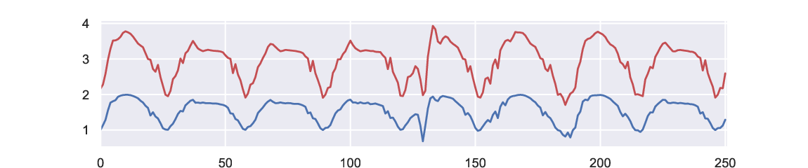

4.3 An Analytic Solution for Bee World
In this section, we will analyse Bee World so that we can compare the ESN solution to results that we can prove. To make our own lives easier, we consider a smooth version of Bee World, rather than the discrete time version solved by the ESN, so that we can formulate Bee World as a control problem that admits a solution via the Euler-Lagrange equation. We have the control system
where is the controller dependant on and . Then we have a cost function
where is the penalty term for using the control and is the nectar function. In the above formulation of Bee World
where . Then the objective is to find
We can see that is not a well defined function so we will introduce the family of functions
where , and notice that approaches pointwise as . Next, we recall that the stationary points (including the minimum) of the integral functional
all satisfy the Euler-Lagrange equation
So, we let
then
which we can reformulate as a dynamical system
| (17) |
whose solutions are stationary points of the integral functional. For small , we approach the Bee World problem. We took , , initial position , and initial velocity then simulated a trajectory of the ODE using scipy.integrate.odeint. We plotted this in Figure 3. The average nectar collected by under this policy was approximately 1.60.

5 Application to Stochastic Control
ESNs have shown remarkable promise in solving problems in mathematical finance - including by [23], [24], and [25] who used an ESN to predict the future values of stock prices. [26] used an ESN to learn the solution to a credit rating problem and [27] used an ESN to forecast exchange rates, comparing the results to forecasts made with an ARMA model. In this section we will introduce a stochastic optimal control problem arising in the market making problem. We will solve this problem analytically, and compare this to the solution obtained by a reinforcement learning agent supported by an ESN.
5.1 A Market Making Problem
We consider a stochastic control problem inspired by the motivations of a market maker acting in a general financial market. In practice the specific role of a market maker depends on the particular market, but we consider a market maker who provides liquidity to other market participants by quoting prices at which they are willing to sell (ask) and buy (bid) an asset. By setting the ask price higher than the bid price in general they can profit from the difference when they receive both a buy and sell order at these prices. However, the market maker faces risk, since if they buy a quantity of the asset the market price might move against them before they are able to find a seller.
The market making problem is a complex one, and has been studied extensively since the publication of the paper by [28]. The paper of [29] gives a good overview of much of this work. We consider a stylised version of this problem that focuses on inventory management without considering explicit optimal quoting strategies. We consider that a market maker acting relatively passively around the market price in ordinary conditions would expect to observe a random demand for buy and sell orders. If as a result of random fluctuations they find their inventory has drifted away from zero, they would set prices more competitively on either the ask or bid side to encourage trades to balance their position. Very broadly the conclusions of work on the market making problem are that there is a price to be paid to exert control over the inventory process and bring inventories closer to zero.
Motivated by this insight, we consider the market maker’s inventory to be a stochastic process with dynamics
where is a standard Brownian motion.
The parameter measures the volatility of the incoming order flow, and is the control process by which the market maker adds drift into their order flow by moving their bid and ask quotes. Naturally, there is a cost involved in applying the control, and a further cost to holding inventory away from zero. We introduce parameters and to quantify these effects and model the market maker’s profit as a stochastic process solving
where is the rate of profit the market maker would achieve from the bid-ask spread if they did not have concerns about the asset price movements. We consider the case where the market maker seeks to maximise their long run discounted profit
where is the expectation with the process started at . We can show that the market maker’s value function and optimal control are
| (18) |
where
Further, the inventory process , when controlled by the optimal control is given by the Ornstein-Uhlenbeck process
whose stationary distribution is a Gaussian .
We observe that this is an infinite horizon, Linear-Quadratic regulator (LQR) type problem, a class of problems which have a long history in the control literature, and more recently have been systematically studied in the reinforcement learning literature. Recent work on online learning for the LQR problem (e.g. [30, 31, 32]) has considered a range of variants of the LQR problem, including cases with uncertainty on the both the dynamics and the reward, and where the state variable may only be partially observed. However most of these approaches work in the setting of model-based learning approaches: that is, they attempt to learn a “model” of the world, and therefore exploit the fact that the LQR structure is known and can be learned from the data; in comparison, [30] still rely on the LQR structure, but do not directly try to learn the “model” of the world. The paper [33] analyses the difference between model-based and model-free approaches to the LQR problem, showing that one should expect an exponential separation between model-based and model-free approaches. In this context, our approach, which does not assume the LQR structure, can also be compared to model-free approaches, such as the classical work of [34], which takes a -learning approach.
5.2 Discretised problem
To turn this into a problem into one that can be used to train an Echo State Network we reformulate it in discrete time; we consider a process such that
where are a sequence of i.i.d. random variables for each , and is the time increment. The control is now a sequence . The profit function satisfies and
and the market maker seeks to maximise the value function
over choices of the control where is the expectation with the process started at .
It can be shown that in the limit as , the optimal control and value function for this problem converge precisely to the optimal control and value function in the continuous case.
We state here the results in the case , the value we will use for the application of the Echo State Network below. Writing , we find in this case that the value function and optimal control are given by
where
.
The process controlled by is Markovian, and has transition operator
It is straightforward to verify that the Gaussian probability density function
| (19) |
is a fixed point of and hence that the controlled process has stationary distribution .
5.3 Solving the Market Making Problem with an ESN
In this section, we seek to solve the the market making problem with a reinforcement learning algorithm supported by an ESN. In this set up, we assume the market maker has no knowledge of the cost function, and no knowledge of the effect of executing an action. The agent must execute a variety of actions in a variety of states to learn about the environment and the effect of its actions. Then, the market maker makes reasonable changes to its policy to arrive at a policy that reduces the long term costs of operation. The policy obtained by the reinforcement learning approach is compared to the optimal policy derived with full knowledge of the system.
5.3.1 Approximating the value functional
For the purpose of running the simulation, we let the cost of operating the control , the cost of straying from the origin , the timestep , and the volatility parameter . We take the baseline profit parameter . The inventory held, and action taken, by the market maker at time will be denoted and respectively. A sequence of (inventory, action) pairs will be denoted with . The value functional for the market maker problem is defined
where is the reward functional
is the shift operator, and is the discount factor representing the relative importance of near and long term costs. We can see after a simple rearrangement that
so is the unique fixed point of the contraction mapping defined by
as discussed in Section 3. Thus, by Theorem 3.6, we can approximate the value function using an ESN trained by regularised least squares if the (inventory, action) pairs are the realisation of a stationary ergodic process. Consequently, we sought an initial policy such that the process comprising the inventory-action pairs under policy is stationary and ergodic. In particular, we chose
| (20) |
with a constant representing the rate of exponential drift toward and . We ran this policy for 10000 time steps, and recorded the pairs along with the rewards . Next, we set up an ESN of dimension , with reservoir matrix, input matrix, and bias populated with i.i.d uniform random variables . was then multiplied by a scaling factor such that the 2-norm of satisfies . As in the previous example we chose to be the ReLU activation function. We then computed reservoir states
starting with an initial reservoir state . An arbitrary reservoir state then encodes the left infinite sequence of (inventory,action) pairs . We seek an expression for the value of the reservoir state by solving the least squares problem
(using the singular value decomposition) where is the matrix with th column is
and is the vector of observations where the th entry is the reward , and is the regularisation parameter which we set to 1e-6. We also chose . In practice, the discount factor is usually much larger. With this, we obtain an expression for value of the reservoir state given by . The results of this policy are shown in Figures 4 and 5. The procedure which estimates the value function and improves upon the policy is described in Algorithm 4.


5.3.2 Updating the policy
We sought to create a new and improved policy based on the observations of under the initial policy using a naïve approach. At each time step, we consider 100 trial actions drawn from the standard normal distribution and compute
where is the (inventory, action) pair , and is trial action. For each , we compute to obtain the predicted value of executing action . We then choose to execute the action with the greatest predicted value, and update the reservoir state using this (inventory, action) pair . This defines our new policy. We ran this new policy for 10,000 time steps and illustrated the results in Figures 6(a), and 6(b).


5.4 Comparison between the analytic and learned solutions
The one step reinforcement learning algorithm did not perfectly replicate the analytically derived optimal control, but has moved in a promising direction. We can see in Figure 6(a) that the inventory process under the improved policy produces (inventory, action) pairs that have some scatter relative to the optimal policy indicated by the red straight line. This suggests that the market maker trained by reinforcement learning is behaving well in some average sense, despite performing many sub-optimal actions. It also appears that the the reinforcement learning algorithm uses the control more aggressively than is optimal. This sub-optimal control results in greater costs than the optimal control. In particular the average cost incurred under the improved policy is 2.65, while the average cost under the the analytically derived optimal policy is .
Despite these sub-optimal moves, it seems that the inventory process learned by the market maker has an invariant measure that closely matches the optimal invariant measure. It is reassuring to see that an invariant measure appears, at least numerically, to exist, because the controlled process is assumed to be stationary and ergodic (and therefore admits an invariant measure) in Theorem 3.6.
It is also worth noting that the inventory process, controlled either by the ESN or the optimal control, has support on , which is not a compact space. Therefore, the conditions of Theorem 3.6 don’t technically hold. However, the numerical results here suggest that the ESN has learned the value functional adequately well, suggesting that Theorem 3.6 may hold under relaxed conditions. Of course, realisations of the stochastic processes always explore only bounded subsets of .
6 Conclusions and future work
In this paper we have presented three novel mathematical results concerning Echo State Networks trained on data drawn from a stationary ergodic process. The first applies to offline supervised learning. The theorem states that, given a target function, enough training data and a large enough ESN, the least squares training procedure will yield an arbitrarily good approximation to the target function. The second result applies to an agent performing a stochastic policy . After the agent has collected enough training data, and given a sufficiently large ESN, the least squares training procedure will yield an arbitrarily good approximation to the value function associated to the policy . The third result is relevant to online reinforcement learning. Though the result is quite preliminary, the lemma is introduced with the intention of developing online algorithms (inspired by Q-learning) to learn the optimal policy for non-Markovian problems.
We demonstrated the second result (which generalises the first) on a deterministic control problem (Bee World) and a stochastic control problem (the market making problem). We chose these ‘toy model’ problems to understand the performance of the algorithm completely in cases that are solvable analytically, although these optimal solutions themselves are not entirely trivial. The reinforcement learning algorithm we use to improve the policy in both Bee World and the market making problem is extremely simple. It is essentially one iteration of an -greedy policy [35], with set to 0. Despite the simplicity of the algorithm, the single iteration considerably improved the policy, resulting in a reasonable approximation to the optimal policy.
It therefore seems a natural direction of future work to develop more sophisticated learning algorithms. Notably the linear upper confidence bound (linUCB) algorithm [35] has a linear structure that fits cleanly into the the linear training framework of the ESN. As this work develops, it will become essential to have a rigorous framework describing the relationship between filters, functionals, random processes and reinforcement learning. The theory presented in this paper tentatively connects these objects using ideas from Markov Decision Processes, but the theory is far from complete.
Acknowledgements
Allen Hart and Kevin Olding are funded through the EPSRC Centre for Doctoral Training in Statistical Applied Mathematics at Bath (SAMBa), grant number EP/L015684/1.
We thank Jeremy Worsfold for insights about reinforcement learning and the linUCB algorithm, and for refactoring the Bee World code. We also thank Adam White for useful discussions about reinforcement learning settings.
References
- [1] H. Jaeger, The “echo state” approach to analysing and training recurrent neural networks, GMD-Report 148, German National Research Institute for Computer Science (01 2001).
- [2] W. Maass, T. Natschläger, H. Markram, Real-time computing without stable states: A new framework for neural computation based on perturbations, Neural Computation 14 (11) (2002) 2531–2560. doi:10.1162/089976602760407955.
- [3] M. Schlegel, A. Jacobsen, M. Zaheer, A. Patterson, A. White, M. White, General value function networks, arXiv:1807.06763 (2018).
- [4] L. Gonon, L. Grigoryeva, J.-P. Ortega, Approximation bounds for random neural networks and reservoir systems, arXiv:2002.05933 (2020).
- [5] M. Lukoševičius, H. Jaeger, Reservoir computing approaches to recurrent neural network training, Computer Science Review 3 (3) (2009) 127 – 149. doi:https://doi.org/10.1016/j.cosrev.2009.03.005.
- [6] M. Lukoševičius, H. Jaeger, B. Schrauwen, Reservoir computing trends, Künstliche Intelligenz. 26 (4) (2012) 365–371.
- [7] A. Rodan, P. Tino, Minimum complexity echo state network, IEEE transactions on neural networks 22 (1) (2011) 131–144.
- [8] F. Triefenbach, A. Jalalvand, B. Schrauwen, J.-P. Martens, Phoneme recognition with large hierarchical reservoirs, in: J. D. Lafferty, C. K. I. Williams, J. Shawe-Taylor, R. S. Zemel, A. Culotta (Eds.), Advances in Neural Information Processing Systems 23, Curran Associates, Inc., 2010, pp. 2307–2315.
- [9] H. Jaeger, H. Haas, Harnessing nonlinearity: Predicting chaotic systems and saving energy in wireless communication, Science 304 (5667) (2004) 78–80. arXiv:https://science.sciencemag.org/content/304/5667/78.full.pdf, doi:10.1126/science.1091277.
- [10] I. Szita, V. Gyenes, A. Lőrincz, Reinforcement learning with echo state networks, in: S. D. Kollias, A. Stafylopatis, W. Duch, E. Oja (Eds.), Artificial Neural Networks – ICANN 2006, Springer Berlin Heidelberg, Berlin, Heidelberg, 2006, pp. 830–839.
- [11] S. Peitz, K. Bieker, On the universal transformation of data-driven models to control systems, arXiv:2102.04722 (2021).
- [12] A. Saxe, P. W. Koh, Z. Chen, M. Bhand, B. Suresh, A. Ng, On random weights and unsupervised feature learning, In Proceedings of the 28th International Conference on Machine Learning (2011).
- [13] L. Grigoryeva, J.-P. Ortega, Echo state networks are universal, Neural Networks 108 (2018) 495 – 508. doi:https://doi.org/10.1016/j.neunet.2018.08.025.
- [14]
L. Grigoryeva, J.-P. Ortega,
Differentiable reservoir
computing, Journal of Machine Learning Research 20 (179) (2019) 1–62.
URL http://jmlr.org/papers/v20/19-150.html - [15]
K. McGoff, S. Mukherjee, N. Pillai,
Statistical inference for dynamical
systems: A review, Statist. Surv. 9 (2015) 209–252.
doi:10.1214/15-SS111.
URL https://doi.org/10.1214/15-SS111 - [16] A. Khaleghi, D. Ryabko, Clustering piecewise stationary processes, in: 2020 IEEE International Symposium on Information Theory (ISIT), 2020, pp. 2753–2758. doi:10.1109/ISIT44484.2020.9174045.
- [17]
A. Hart, J. Hook, J. Dawes,
Embedding
and approximation theorems for echo state networks, Neural Networks 128
(2020) 234 – 247.
doi:https://doi.org/10.1016/j.neunet.2020.05.013.
URL http://www.sciencedirect.com/science/article/pii/S0893608020301830 - [18]
A. G. Hart, J. L. Hook, J. H. Dawes,
Echo
state networks trained by tikhonov least squares are approximators
of ergodic dynamical systems, Physica D: Nonlinear Phenomena (2021)
132882doi:https://doi.org/10.1016/j.physd.2021.132882.
URL https://www.sciencedirect.com/science/article/pii/S0167278921000403 - [19] A. Benveniste, M. Métivier, P. Prioure, Adaptive Algorithms and Stochastic Approximations, Springer-Verlag, 1990.
- [20] V. S. Borkar, Stochastic Approximation: A Dynamical Systems Viewpoint, Hindustan Book Agency, 2009.
- [21] F. S. Melo, M. I. Ribeiro, Q-learning with linear function approximation, in: N. H. Bshouty, C. Gentile (Eds.), Learning Theory, Springer Berlin Heidelberg, Berlin, Heidelberg, 2007, pp. 308–322.
- [22] Z. Chen, S. Zhang, T. T. Doan, S. T. Maguluri, J.-P. Clarke, Performance of q-learning with linear function approximation: Stability and finite-time analysis, arXiv:1905.11425 (2019).
- [23]
X. Lin, Z. Yang, Y. Song,
Short-term
stock price prediction based on echo state networks, Expert Systems with
Applications 36 (3, Part 2) (2009) 7313 – 7317.
doi:https://doi.org/10.1016/j.eswa.2008.09.049.
URL http://www.sciencedirect.com/science/article/pii/S0957417408006519 - [24]
H. Zhang, J. Liang, Z. Chai,
Stock prediction based on
phase space reconstruction and echo state networks, Journal of Algorithms &
Computational Technology 7 (1) (2013) 87–100.
arXiv:https://doi.org/10.1260/1748-3018.7.1.87, doi:10.1260/1748-3018.7.1.87.
URL https://doi.org/10.1260/1748-3018.7.1.87 - [25]
J. Dan, W. Guo, W. Shi, B. Fang, T. Zhang,
Deterministic echo state networks
based stock price forecasting, Abstract and Applied Analysis 2014 (2014)
137148.
doi:10.1155/2014/137148.
URL https://doi.org/10.1155/2014/137148 - [26] J. Bozsik, Z. Ilonczai, Echo state network-based credit rating system, in: 2012 4th IEEE International Symposium on Logistics and Industrial Informatics, 2012, pp. 185–190.
- [27] L. Maciel, F. Gomide, D. Santos, R. Ballini, Exchange rate forecasting using echo state networks for trading strategies, in: 2014 IEEE Conference on Computational Intelligence for Financial Engineering Economics (CIFEr), 2014, pp. 40–47.
- [28]
M. Avellaneda, S. Stoikov,
High-frequency trading in a
limit order book, Quantitative Finance 8 (3) (2008) 217–224.
arXiv:https://doi.org/10.1080/14697680701381228, doi:10.1080/14697680701381228.
URL https://doi.org/10.1080/14697680701381228 - [29]
O. Guéant, Optimal
market making, Applied Mathematical Finance 24 (2) (2017) 112–154.
arXiv:https://doi.org/10.1080/1350486X.2017.1342552, doi:10.1080/1350486X.2017.1342552.
URL https://doi.org/10.1080/1350486X.2017.1342552 - [30] M. Fazel, R. Ge, S. Kakade, M. Mesbahi, Global Convergence of Policy Gradient Methods for the Linear Quadratic Regulator, in: International Conference on Machine Learning, PMLR, 2018, pp. 1467–1476, iSSN: 2640-3498.
- [31] Z. Mhammedi, D. J. Foster, M. Simchowitz, D. Misra, W. Sun, A. Krishnamurthy, A. Rakhlin, J. Langford, Learning the linear quadratic regulator from nonlinear observations, arXiv:2010.03799 (2020).
- [32]
S. Dean, H. Mania, N. Matni, B. Recht, S. Tu,
On the Sample
Complexity of the Linear Quadratic Regulator, Foundations of
Computational Mathematics 20 (4) (2020) 633–679.
doi:10.1007/s10208-019-09426-y.
URL https://doi.org/10.1007/s10208-019-09426-y - [33]
S. Tu, B. Recht, The Gap
Between Model-Based and Model-Free Methods on the Linear
Quadratic Regulator: An Asymptotic Viewpoint, in: Conference on
Learning Theory, PMLR, 2019, pp. 3036–3083, iSSN: 2640-3498.
URL http://proceedings.mlr.press/v99/tu19a.html - [34] S. Bradtke, B. Ydstie, A. Barto, Adaptive linear quadratic control using policy iteration, in: Proceedings of 1994 American Control Conference - ACC ’94, Vol. 3, 1994, pp. 3475–3479 vol.3. doi:10.1109/ACC.1994.735224.
- [35] R. S. Sutton, A. G. Barto, Reinforcement Learning: An Introduction, MIT-press, 2015.