跳到论文正文
W Papers独立论文阅读器 arXiv:2102.06201 论文正文 计算阅读时间 · 0%
引用这篇论文根据当前论文元数据生成,正式投稿前建议核对。


License: arXiv.org perpetual non-exclusive license
arXiv:2102.06201v1 [cond-mat.str-el] 11 Feb 2021

TSTG I: Single-Particle and Many-Body Hamiltonians and Hidden Non-local Symmetries of Trilayer Moiré Systems with and without Displacement Field

Dumitru Călugăru Thanks: These authors contributed equally. Affiliation: Department of Physics, Princeton University, Princeton, New Jersey 08544, USA    Fang Xie Affiliation: Department of Physics, Princeton University, Princeton, New Jersey 08544, USA    Zhi-Da Song Affiliation: Department of Physics, Princeton University, Princeton, New Jersey 08544, USA    Biao Lian Affiliation: Department of Physics, Princeton University, Princeton, New Jersey 08544, USA    Nicolas Regnault Thanks: These authors contributed equally. Affiliation: Department of Physics, Princeton University, Princeton, New Jersey 08544, USA Affiliation: Laboratoire de Physique de l’Ecole normale superieure, ENS, Université PSL, CNRS, Sorbonne Université, Université Paris-Diderot, Sorbonne Paris Cité, Paris, France    B. Andrei Bernevig Thanks: These authors contributed equally. Affiliation: Department of Physics, Princeton University, Princeton, New Jersey 08544, USA
August 11, 2026
Abstract

We derive the Hamiltonian for trilayer moiré systems with the Coulomb interaction projected onto the bands near the charge neutrality point. Motivated by the latest experimental results, we focus on the twisted symmetric trilayer graphene (TSTG) with a mirror-symmetry with respect to the middle layer. We provide a full symmetry analysis of the non-interacting Hamiltonian with a perpendicular displacement field coupling the band structure made otherwise of the twisted bilayer graphene (TBG) and the high velocity Dirac fermions, and we identify a hidden non-local symmetry of the problem. In the presence of this displacement field, we construct an approximate single-particle model, akin to the tripod model for TBG, capturing the essence of non-interacting TSTG. We also derive more quantitative perturbation schemes for the low-energy physics of TSTG with displacement field, obtaining the corresponding eigenstates. This allows us to obtain the Coulomb interaction Hamiltonian projected in the active band TSTG wavefunctions and derive the full many-body Hamiltonian of the system. We also provide an efficient parameterization of the interacting Hamiltonian. Finally, we show that the discrete symmetries at the single-particle level promote the U⁡(2)×U⁡(2)\mathrm{U}\left(2\right)\times\mathrm{U}\left(2\right) spin-valley symmetry to enlarged symmetry groups of the interacting problem under different limits. The interacting part of the Hamiltonian exhibits a large U⁡(4)×U⁡(4)×U⁡(4)×U⁡(4)\mathrm{U}\left(4\right)\times\mathrm{U}\left(4\right)\times\mathrm{U}\left(4\right)\times\mathrm{U}\left(4\right) symmetry in the chiral limit. Moreover, by identifying a new symmetry which we dub spatial many-body charge conjugation, we show that the physics of TSTG is symmetric around charge neutrality.

I Introduction

As a result of its chemical versatility, an impressive number of stable carbon allotropes has been synthesized and investigated. One of the newest addition to the family, twisted bilayer graphene (TBG), has generated a lot of excitement in the condensed matter community. The resulting van der Waals heterostructure obtained by stacking two graphene layers with a small relative twist has been theoretically shown to host flat bands at certain so-called magic angles Lopes dos Santos et al. 2007; Suárez Morell et al. 2010; Bistritzer and MacDonald 2011. Subsequent experimental studies have revealed various correlated insulating and superconducting phases in TBG near the first magic angle θTBG≈1.05∘\theta_{\mathrm{TBG}}\approx 1.05^{\circ}, using both transport Cao et al. 2018; Cao et al. 2020a; Chen et al. 2020a; Liu et al. 2020a; Lu et al. 2019; Lu et al. 2020; Park et al. 2020a; Polshyn et al. 2019; Saito et al. 2020; Saito et al. 2021; Serlin et al. 2020; Stepanov et al. 2020; Wu et al. 2020a; Yankowitz et al. 2019 and spectroscopy Choi et al. 2019; Choi et al. 2020; Kerelsky et al. 2019; Nuckolls et al. 2020; Wong et al. 2020; Xie et al. 2019; Jiang et al. 2019; Choi et al. 2021 experiments. In turn, these findings have inspired a wealth of theoretical investigations into the rich physics of TBG Kang and Vafek 2019; Seo et al. 2019; Bultinck et al. 2020a; Hejazi et al. 2020; Fernandes and Fu 2021; Fernandes and Venderbos 2020; Venderbos and Fernandes 2018; Potasz et al. 2021; Abouelkomsan et al. 2020; Ahn et al. 2019; Bernevig et al. 2020a; Bernevig et al. 2020b; Bernevig et al. 2020c; Bultinck et al. 2020b; Cao et al. 2020b; Cea and Guinea 2020; Christos et al. 2020; Classen et al. 2019; Da Liao et al. 2019; Da Liao et al. 2020; Dai et al. 2016; Dodaro et al. 2018; Efimkin and MacDonald 2018; Eugenio and Dag 2020; González and Stauber 2019; Guinea and Walet 2018; Guo et al. 2018; Hejazi et al. 2019a; Hejazi et al. 2019b; Huang et al. 2019; Huang et al. 2020; Isobe et al. 2018; Jain et al. 2016; Julku et al. 2020; Kang and Vafek 2018; Kang and Vafek 2020; Kennes et al. 2018; Khalaf et al. 2020; König et al. 2020; Koshino et al. 2018; Ledwith et al. 2020; Lewandowski et al. 2020; Lian et al. 2019; Lian et al. 2020a; Lian et al. 2020b; Liu et al. 2012; Liu et al. 2018; Liu et al. 2019a; Liu and Dai 2021; Liu et al. 2021; Ochi et al. 2018; Padhi et al. 2020; Peltonen et al. 2018; Po et al. 2018; Po et al. 2019; Repellin et al. 2020; Repellin and Senthil 2020; Roy and Juričić 2019; Soejima et al. 2020; Song et al. 2019; Song et al. 2020; Tarnopolsky et al. 2019; Thomson et al. 2018; Uchida et al. 2014; Vafek and Kang 2020; Venderbos and Fernandes 2018; Wang et al. 2020; van Wijk et al. 2015; Wilson et al. 2020; Wu et al. 2018; Wu et al. 2019a; Wu et al. 2019b; Wu and Das Sarma 2020; Xie et al. 2020a; Xie et al. 2020b; Xie and MacDonald 2020a; Xie and MacDonald 2020b; Xu and Balents 2018; Xu et al. 2018; You and Vishwanath 2019; Yuan and Fu 2018; Zhang et al. 2020a; Zou et al. 2018.

Such progress on both the experimental and theoretical fronts has triggered a large effort into extending the family of moiré superlattices, promoting them as some of the most promising platforms to engineer strongly correlated quantum phases Kennes et al. 2020. The main driving force in investigating moiré materials beyond TBG is often the different band tunability properties of the former. Consequently, the extension to twisted multilayer graphene has already been widely studied theoretically Burg et al. 2019; Cao et al. 2020b; Carr et al. 2020a; Carr et al. 2020b; Cea et al. 2019; García-Ruiz et al. 2020; Haddadi et al. 2020; Khalaf et al. 2019; Lei et al. 2020; Li et al. 2019; Liu et al. 2019b; Lopez-Bezanilla and Lado 2020; Mora et al. 2019; Park et al. 2020b; Suárez Morell et al. 2013; Wu et al. 2020b; Zhang et al. 2020b; Zhu et al. 2020a; Zhu et al. 2020b. Later experiments have also revealed equally intriguing superconducting and insulating phases in moiré systems with three Chen et al. 2019a; Chen et al. 2019b; Chen et al. 2020b; Hao et al. 2021; Park et al. 2021; Polshyn et al. 2020; Shi et al. 2020; Tsai et al. 2020 or four Burg et al. 2019; Burg et al. 2020; Cao et al. 2020c; Liu et al. 2020b; Shen et al. 2020 graphene layers.

Among the simplest moiré graphene systems beyond TBG, twisted symmetric trilayer graphene (TSTG) Mora et al. 2019; Khalaf et al. 2019 has been recently experimentally realized in Refs. Park et al. 2021; Hao et al. 2021. TSTG is comprised of three AAA-stacked graphene layers in which the middle layer is twisted slightly relative to the top and bottom ones. For this type of stacking, which was shown to be energetically favorable Carr et al. 2020a, the system is mirror-symmetric with respect to reflections in the plane of the middle graphene layer. As such, TSTG decouples into mirror-symmetry sectors in the absence of interactions Khalaf et al. 2019 and can be thought of as being comprised of a “TBG-like” contribution with an interlayer coupling effectively enhanced by a factor of 2\sqrt{2} Khalaf et al. 2019, and a high-velocity Dirac fermion Carr et al. 2020a. The renormalized interlayer coupling of the TBG fermions leads to a rescaling of the first magic angle by the same amount, yielding θTSTG≈1.56∘\theta_{\mathrm{TSTG}}\approx 1.56^{\circ} in agreement with the recent experimental observations Park et al. 2021; Hao et al. 2021. However, despite being independent at the single-particle level, the two mirror-symmetry sectors of TSTG are coupled by the electron-electron interactions, pointing to a potentially richer correlated physics compared to TBG. Moreover, the TBG and Dirac cone contributions can be hybridized by the application of a perpendicular displacement field Carr et al. 2020a; Hao et al. 2021; Lei et al. 2020; Park et al. 2021. This provides another knob to experimentally tune the TSTG band structure.

To unveil the above-mentioned richness, we here investigate both the single-particle Bistritzer-MacDonald model and the interaction Coulomb Hamiltonian for TSTG at the first magic angle, with or without displacement field. The main result of this paper is to derive expressions and effective models, as well as the symmetries of the interacting TSTG Hamiltonian under different limits. For this purpose, we discuss the discrete symmetries of the single-particle problem and show how they promote the U⁡(2)×U⁡(2)\mathrm{U}\left(2\right)\times\mathrm{U}\left(2\right) valley-spin rotation symmetry to enhanced rotation symmetries of the interacting problem. We uncover new non-local hidden symmetries of the system at both the single-particle and many-body level. At the same time, we also provide a series of approximations for the single-particle energy spectrum of TSTG in the presence of displacement field and show how it can be obtained in terms of the TBG flat band wave functions, whose properties have been extensively studied in Refs. Song et al. 2019; Bernevig et al. 2020a; Bernevig et al. 2020b; Song et al. 2020. Despite the addition of a Dirac degree of freedom, we find the symmetries of the many-body TSTG Hamiltonian to be enhanced from those of TBG.

The article is organized as follows. In section II, we review the single-particle TSTG Hamiltonian and derive a low-energy approximation. We then investigate its symmetries (including the hidden non-local symmetries) in section III under various limits with or without displacement field. Section IV focuses on the single-particle energy spectrum. We show that an approximate tripod model correctly captures the salient features of TSTG and we derive the single-particle projected Hamiltonian. Section V is devoted to the interacting Hamiltonian, deriving the expression of the projected Coulomb interaction for the TSTG model. Finally, we discuss in section VI the symmetries of the fully interacting projected TSTG Hamiltonian in several limits.

II Single-particle Hamiltonian

First, we outline the derivation of a Bistritzer-MacDonald model for TSTG Bistritzer and MacDonald 2011. A more detailed exposition is provided in Appendix A.1. The main result of this section is to show that the TSTG Hamiltonian can be thought as a sum between a TBG Hamiltonian (with renormalized interlayer hopping amplitudes) and an independent Dirac cone Hamiltonian. Furthermore, we show that the hybridization between the TBG and Dirac cone fermions can be tuned by the addition of a perpendicular displacement field Hao et al. 2021; Park et al. 2021.

II.1 Notations

(a)
(b)
Figure 1: The Moiré Lattice of TSTG. Panel (a) illustrates the BZs of the graphene layers, which are plotted in blue for the top (l=3l=3) and bottom (l=1l=1) layers and in orange for the middle layer (l=2l=2). The KK (K′K^{\prime}) point are located at 𝐊+\mathbf{K}_{+} (−𝐊+-\mathbf{K}_{+}) for the top and bottom layer and at 𝐊−\mathbf{K}_{-} (−𝐊−-\mathbf{K}_{-}). When the twist angle θ\theta is small, an approximate translation symmetry arises, allowing us to define the MBZ (dashed black hexagon). The 𝒬±\mathcal{Q}_{\pm} lattices are shown in panel (b). Inside the first MBZ (defined as the hexagonal region around ΓM\Gamma_{M}) we have plotted the regions AηiA_{\eta}^{i} defined in eq. 9 as filled blue (η=+\eta=+) and orange (η=−\eta=-) circular sectors.

In the case of graphene, the twisted trilayer geometry was considered theoretically in Refs. Mora et al. 2019; Khalaf et al. 2019. Throughout this paper, however, we will follow the notation of Refs. Song et al. 2019; Bernevig et al. 2020a; Song et al. 2020; Bernevig et al. 2020b; Lian et al. 2020a; Bernevig et al. 2020c; Xie et al. 2020b. We take a^𝐩,α,s,l†\hat{a}^{\dagger}_{\mathbf{p},\alpha,s,l} to represent the fermion operator in the plane wave basis for graphene layer l=1,2,3l=1,2,3 (corresponding to the bottom, middle, and top layers, respectively). The momentum 𝐩\mathbf{p} is measured from the Γ\Gamma point of the monolayer graphene Brillouin Zone (BZ), as shown in fig. 1a, α=A,B\alpha=A,B is the sublattice index, and s=↑,↓s=\uparrow,\downarrow denotes the projection of the electron spin along the z^\hat{z} direction. Within each graphene layer, the low-energy physics is concentrated around the two valleys, KK and K′K^{\prime}, labeled by η=±1\eta=\pm 1 and located at momenta η​𝐊l\eta\mathbf{K}_{l}. Owing to the mirror-symmetric arrangement of the graphene layers, we can introduce 𝐊+≡𝐊1=𝐊3\mathbf{K}_{+}\equiv\mathbf{K}_{1}=\mathbf{K}_{3} to be the KK point in the bottom and top layer graphene BZ (l=1,3l=1,3), and 𝐊−≡𝐊2\mathbf{K}_{-}\equiv\mathbf{K}_{2}, to be the KK point of the middle layer graphene BZ (l=2l=2).

For convenience, we define the momenta 𝐪j=C3​zj−1​(𝐊+−𝐊−)\mathbf{q}_{j}=C_{3z}^{j-1}\left(\mathbf{K}_{+}-\mathbf{K}_{-}\right), where j=1,2,3j=1,2,3 and C3​zC_{3z} represents the three-fold rotation transformation around the z^\hat{z} axis. We can then define a moiré BZ (MBZ) for the TSTG moiré lattice 𝒬0=ℤ​𝐛M​1+ℤ​𝐛M​2\mathcal{Q}_{0}=\mathbb{Z}\mathbf{b}_{M1}+\mathbb{Z}\mathbf{b}_{M2}, which is generated by the reciprocal vectors 𝐛M​i=𝐪3−𝐪i\mathbf{b}_{Mi}=\mathbf{q}_{3}-\mathbf{q}_{i} (i=1,2i=1,2). We also define two shifted momentum lattices 𝒬±=±𝐪1+𝒬0\mathcal{Q}_{\pm}=\pm\mathbf{q}_{1}+\mathcal{Q}_{0}, which together form a honeycomb lattice, as seen in fig. 1b. We can then introduce the low-energy fermion operators defined on the moiré lattice as a^𝐤,𝐐,η,α,s,l†≡a^η​𝐊l+𝐤−𝐐,α,s,l†\hat{a}^{\dagger}_{\mathbf{k},\mathbf{Q},\eta,\alpha,s,l}\equiv\hat{a}^{\dagger}_{\eta\mathbf{K}_{l}+\mathbf{k}-\mathbf{Q},\alpha,s,l} for 𝐐∈𝒬η,l\mathbf{Q}\in\mathcal{Q}_{\eta,l} with 𝐤\mathbf{k} measured from the ΓM\Gamma_{M} point, and 𝒬η,l=𝒬η\mathcal{Q}_{\eta,l}=\mathcal{Q}_{\eta} for l=1,3l=1,3 and 𝒬η,l=𝒬−η\mathcal{Q}_{\eta,l}=\mathcal{Q}_{-\eta} for l=2l=2.

The expression of the TSTG single-particle Hamiltonian in terms of the a^†\hat{a}^{\dagger} operators given in section A.1 of Appendix A.1 can be simplified by introducing a basis transformation: in the absence of a perpendicular displacement field, a TSTG sample is symmetric under mirror mzm_{z} reflections with respect to the middle graphene layer plane. This allows us to define a set of mirror-symmetric and mirror-antisymmetric operators, which are respectively given by

c^𝐤,𝐐,η,α,s†={12​(a^𝐤,𝐐,η,α,s,3†+a^𝐤,𝐐,η,α,s,1†)𝐐∈𝒬ηa^𝐤,𝐐,η,α,s,2†𝐐∈𝒬−η,\hat{c}^{\dagger}_{\mathbf{k},\mathbf{Q},\eta,\alpha,s}=\begin{cases}\frac{1}{\sqrt{2}}\left(\hat{a}^{\dagger}_{\mathbf{k},\mathbf{Q},\eta,\alpha,s,3}+\hat{a}^{\dagger}_{\mathbf{k},\mathbf{Q},\eta,\alpha,s,1}\right)&\mathbf{Q}\in\mathcal{Q}_{\eta}\\ \hat{a}^{\dagger}_{\mathbf{k},\mathbf{Q},\eta,\alpha,s,2}&\mathbf{Q}\in\mathcal{Q}_{-\eta}\end{cases}, (1)

and

b^𝐤,𝐐,η,α,s†=12​(a^𝐤,𝐐,η,α,s,3†−a^𝐤,𝐐,η,α,s,1†)​𝐐∈𝒬η.\hat{b}^{\dagger}_{\mathbf{k},\mathbf{Q},\eta,\alpha,s}=\frac{1}{\sqrt{2}}\left(\hat{a}^{\dagger}_{\mathbf{k},\mathbf{Q},\eta,\alpha,s,3}-\hat{a}^{\dagger}_{\mathbf{k},\mathbf{Q},\eta,\alpha,s,1}\right)\mathbf{Q}\in\mathcal{Q}_{\eta}. (2)

II.2 Hamiltonian

When written in with the aid of the b^†\hat{b}^{\dagger} and c^†\hat{c}^{\dagger} operators, the single-particle Hamiltonian can be separated into three terms

H^0=H^TBG+H^D+H^U.\hat{H}_{0}=\hat{H}_{\mathrm{TBG}}+\hat{H}_{D}+\hat{H}_{U}. (3)

In eq. 3, the mirror-symmetric low-energy operators give rise to the term

H^TBG=∑𝐤∈MBZη,α,β,s𝐐,𝐐′∈𝒬±[h𝐐,𝐐′(η)​(𝐤)]α​β​c^𝐤,𝐐,η,α,s†​c^𝐤,𝐐′,η,β,s,\hat{H}_{\mathrm{TBG}}=\sum_{\begin{subarray}{c}\mathbf{k}\in\text{MBZ}\\ \eta,\alpha,\beta,s\\ \mathbf{Q},\mathbf{Q}^{\prime}\in\mathcal{Q}_{\pm}\end{subarray}}\left[h^{\left(\eta\right)}_{\mathbf{Q},\mathbf{Q}^{\prime}}\left(\mathbf{k}\right)\right]_{\alpha\beta}\hat{c}^{\dagger}_{\mathbf{k},\mathbf{Q},\eta,\alpha,s}\hat{c}_{\mathbf{k},\mathbf{Q}^{\prime},\eta,\beta,s}, (4)

which is similar to the ordinary TBG Hamiltonian Song et al. 2019; Khalaf et al. 2019, but with a tunneling amplitude which is rescaled by a factor of 2\sqrt{2}, corresponding to

h𝐐,𝐐′(η)​(𝐤)=h𝐐D,η​(𝐤)​δ𝐐,𝐐′+2​h𝐐,𝐐′I,η.h^{\left(\eta\right)}_{\mathbf{Q},\mathbf{Q}^{\prime}}\left(\mathbf{k}\right)=h^{D,\eta}_{\mathbf{Q}}\left(\mathbf{k}\right)\delta_{\mathbf{Q},\mathbf{Q}^{\prime}}+\sqrt{2}h^{I,\eta}_{\mathbf{Q},\mathbf{Q}^{\prime}}. (5)

The first-quantized Hamiltonians h𝐐D,η​(𝐤)h^{D,\eta}_{\mathbf{Q}}\left(\mathbf{k}\right) and h𝐐,𝐐′I,ηh^{I,\eta}_{\mathbf{Q},\mathbf{Q}^{\prime}} from eq. 5, whose exact forms are given in Appendix A.1, denote a Dirac cone contribution with Fermi velocity vFv_{F} folded inside the first MBZ and an interlayer hopping term, respectively. In particular, there are two parameters w0w_{0} and w1w_{1} in h𝐐,𝐐′I,ηh^{I,\eta}_{\mathbf{Q},\mathbf{Q}^{\prime}}, which correspond to the interlayer hoppings at the A​AAA and A​B/B​AAB/BA stacking centers, respectively. Generically, one has 0≤w0<w10\leq w_{0}<w_{1} due to lattice relaxation and corrugation effects Uchida et al. 2014; van Wijk et al. 2015; Dai et al. 2016; Jain et al. 2016; Song et al. 2020. At the same time, the mirror-symmetric operators, which are only defined for 𝐐∈𝒬η\mathbf{Q}\in\mathcal{Q}_{\eta}, correspond to a solitary Dirac cone contribution

H^D=∑𝐤∈MBZη,α,β,s∑𝐐∈𝒬η[h𝐐D,η​(𝐤)]α​β​b^𝐤,𝐐,η,α,s†​b^𝐤,𝐐,η,β,s.\hat{H}_{D}=\sum_{\begin{subarray}{c}\mathbf{k}\in\text{MBZ}\\ \eta,\alpha,\beta,s\end{subarray}}\sum_{\mathbf{Q}\in\mathcal{Q}_{\eta}}\left[h^{D,\eta}_{\mathbf{Q}}\left(\mathbf{k}\right)\right]_{\alpha\beta}\hat{b}^{\dagger}_{\mathbf{k},\mathbf{Q},\eta,\alpha,s}\hat{b}_{\mathbf{k},\mathbf{Q},\eta,\beta,s}. (6)

Additionally, in eq. 3, we have introduced a perpendicular displacement field, which is equivalent to an onsite potential of U/2U/2, 00, −U/2-U/2 in the top, middle, and bottom layers, respectively. The displacement field contribution couples the TBG-like and the Dirac cone fermions giving rise to

H^U=∑𝐤∈MBZη,α,s∑𝐐∈𝒬ηU2(b^𝐤,𝐐,η,α,s†c^𝐤,𝐐,η,α,s+h.c.),\hat{H}_{U}=\sum_{\begin{subarray}{c}\mathbf{k}\in\text{MBZ}\\ \eta,\alpha,s\end{subarray}}\sum_{\mathbf{Q}\in\mathcal{Q}_{\eta}}\frac{U}{2}\left(\hat{b}^{\dagger}_{\mathbf{k},\mathbf{Q},\eta,\alpha,s}\hat{c}_{\mathbf{k},\mathbf{Q},\eta,\alpha,s}+\mathrm{h.c.}\right), (7)

which explicitly breaks the mirror mzm_{z} symmetry. In what follows, we will find it convenient to employ dimensionless units in which momentum (𝐤\mathbf{k}) and energy (EE) are rescaled according to

𝐤→𝐤kθ,E→EvF​kθ,\mathbf{k}\to\frac{\mathbf{k}}{k_{\theta}},\qquad E\to\frac{E}{v_{F}k_{\theta}}, (8)

where kθ=|𝐊+−𝐊−|k_{\theta}=\absolutevalue{\vec{K}_+ - \vec{K}_-}. This essentially amounts to setting vF=1v_{F}=1, as well as |𝐪i|=1\absolutevalue{\vec{q}_i}=1 (i=1,2,3i=1,2,3).

II.3 Low-energy approximation

The low-energy physics of TSTG with displacement field near the magic angle arises from the interplay between the almost flat (i.e. with a bandwidth much smaller than one, in non-dimensional units) bands of H^TBG\hat{H}_{\mathrm{TBG}} and the MBZ-folded high-velocity Dirac cone bands of H^D\hat{H}_{D}. The only states of H^D\hat{H}_{D} which can efficiently perturb and hybridize the flat-band modes of the TBG-like sector are the ones which have an energy significantly smaller than one. As a low-energy approximation, we can thus restrict ourselves to the momentum points where |h𝐐D,η​(𝐤)|≪1\absolutevalue{h_{\vec{Q}}^{D,\eta}\left( \vec{k} \right)}\ll 1 in eq. 6, which is equivalent to 𝐐∈{η​𝐪i}\mathbf{Q}\in\left\{\eta\mathbf{q}_{i}\right\} and 𝐤\mathbf{k} belonging to one of the three zones AηiA^{i}_{\eta} (where i=1,2,3i=1,2,3) defined for each valley η\eta as

Aηi={𝐤∈MBZ∣|𝐤−η​𝐪𝐢|≤Λ}.A^{i}_{\eta}=\left\{\mathbf{k}\in\mathrm{MBZ}\mid\absolutevalue{\vec{k} - \vec{\eta q_i}}\leq\Lambda\right\}. (9)

Effectively, we consider the Dirac cone contribution in the MBZ only within a small distance Λ\Lambda from the Dirac points of H^D\hat{H}_{D}, as shown in fig. 1b. Typically, the cutoff Λ\Lambda is smaller than the gap between the TBG active and passive bands, but bigger than the bandwidth of the flat bands of H^TBG\hat{H}_{\mathrm{TBG}}. For 0≤U≤0.30\leq U\leq 0.3, we find that Λ≤0.2\Lambda\leq 0.2 (see Appendix D.2). With these approximations, we can write the Dirac cone Hamiltonian projected into the low-energy degrees of freedom as

HD=∑η,α,β,s∑i=13∑𝐤∈Aηi[hη​𝐪iD,η​(𝐤)]α​β​b^𝐤,η​𝐪i,η,α,s†​b^𝐤,η​𝐪i,η,β,s,H_{D}=\sum_{\eta,\alpha,\beta,s}\sum_{i=1}^{3}\sum_{\mathbf{k}\in A^{i}_{\eta}}\left[h^{D,\eta}_{\eta\mathbf{q}_{i}}\left(\mathbf{k}\right)\right]_{\alpha\beta}\hat{b}^{\dagger}_{\mathbf{k},\eta\mathbf{q}_{i},\eta,\alpha,s}\hat{b}_{\mathbf{k},\eta\mathbf{q}_{i},\eta,\beta,s}, (10)

which is denoted without the “hat” to distinguish it from the unprojected H^D\hat{H}_{D}.

III Symmetries of the single-particle Hamiltonian

This section outlines the symmetries of the TSTG single-particle Hamiltonian from eq. 3. The reader is referred to Appendix B for a more in-depth discussion. In the case of zero displacement field, TSTG is symmetric under mirror reflections with the mirror plane parallel to the graphene layers, enabling us to discuss the symmetries of the system for each independent mirror-symmetry sector. Finally, we identify which symmetries of TSTG survive the hybridization between the Dirac cone and TBG fermions in presence of the applied displacement field.

III.1 Symmetry transformations

Due to its negligible spin-orbit coupling, single-layer graphene admits a series of spinless symmetry transformations, some of which are inherited by the single-particle TSTG Hamiltonian from eq. 3. To keep the discussion general, we can consider the action of these transformations on a generic fermion operator f^𝐤,𝐐,η,α,s†\hat{f}^{\dagger}_{\mathbf{k},\mathbf{Q},\eta,\alpha,s} defined on the moiré lattice (where f^†=b^†,c^†\hat{f}^{\dagger}=\hat{b}^{\dagger},\hat{c}^{\dagger}). The unitary discrete symmetry transformations C2​zC_{2z}, C3​zC_{3z}, and C2​xC_{2x} respectively denote a two-fold rotation around the z^\hat{z} axis, a three-fold rotation around the z^\hat{z} axis, and a two-fold rotation around the x^\hat{x} axis. Their action on the moiré lattice fermion operators is given by

C2​z​f^𝐤,𝐐,η,α,s†​C2​z−1=∑β(σx)β​α​f^−𝐤,−𝐐,−η,β,s†,C3​z​f^𝐤,𝐐,η,α,s†​C3​z−1=∑β(ei​η​2​π3​σz)β​α​f^C3​z​𝐤,C3​z​𝐐,η,β,s†,C2​x​f^𝐤,𝐐,η,α,s†​C2​x−1=∑β(σx)β​α​f^C2​x​𝐤,C2​x​𝐐,η,β,s†.\begin{split}C_{2z}\hat{f}^{\dagger}_{\mathbf{k},\mathbf{Q},\eta,\alpha,s}C_{2z}^{-1}&=\sum_{\beta}\left(\sigma_{x}\right)_{\beta\alpha}\hat{f}^{\dagger}_{-\mathbf{k},-\mathbf{Q},-\eta,\beta,s},\\ C_{3z}\hat{f}^{\dagger}_{\mathbf{k},\mathbf{Q},\eta,\alpha,s}C_{3z}^{-1}&=\sum_{\beta}\left(e^{i\eta\frac{2\pi}{3}\sigma_{z}}\right)_{\beta\alpha}\hat{f}^{\dagger}_{C_{3z}\mathbf{k},C_{3z}\mathbf{Q},\eta,\beta,s},\\ C_{2x}\hat{f}^{\dagger}_{\mathbf{k},\mathbf{Q},\eta,\alpha,s}C_{2x}^{-1}&=\sum_{\beta}\left(\sigma_{x}\right)_{\beta\alpha}\hat{f}^{\dagger}_{C_{2x}\mathbf{k},C_{2x}\mathbf{Q},\eta,\beta,s}.\end{split} (11)

We also introduce the spinless mirror symmetry mzm_{z} acting on the two fermion flavors as

mz​c^𝐤,𝐐,η,α,s†​mz−1=c^𝐤,𝐐,η,α,s†,mz​b^𝐤,𝐐,η,α,s†​mz−1=−b^𝐤,𝐐,η,α,s†.\begin{split}m_{z}\hat{c}^{\dagger}_{\mathbf{k},\mathbf{Q},\eta,\alpha,s}m_{z}^{-1}=\hat{c}^{\dagger}_{\mathbf{k},\mathbf{Q},\eta,\alpha,s},\\ m_{z}\hat{b}^{\dagger}_{\mathbf{k},\mathbf{Q},\eta,\alpha,s}m_{z}^{-1}=-\hat{b}^{\dagger}_{\mathbf{k},\mathbf{Q},\eta,\alpha,s}.\end{split} (12)

Finally, we define the action of the spinless anti-unitary time-reversal operator

T​f^𝐤,𝐐,η,α,s†​T−1=f^−𝐤,−𝐐,−η,α,s†.T\hat{f}^{\dagger}_{\mathbf{k},\mathbf{Q},\eta,\alpha,s}T^{-1}=\hat{f}^{\dagger}_{-\mathbf{k},-\mathbf{Q},-\eta,\alpha,s}. (13)

The above operators represent commuting symmetries of the single-layer graphene Hamiltonian. In addition, there are three useful transformations which give rise to anticommuting symmetries, reflecting a relation between the positive and negative energy spectra of the Hamiltonians: a unitary particle-hole symmetry PP and two chiral transformations CC and C′C^{\prime}, the latter two being only valid for different limits of the values of w0/w1w_{0}/w_{1} (respectively w0=0w_{0}=0 and w1=0w_{1}=0). Their action on the moiré lattice fermions is given by

P​f^𝐤,𝐐,η,α,s†​P−1=ζ𝐐​f^−𝐤,−𝐐,η,α,s†,C​f^𝐤,𝐐,η,α,s†​C−1=(σz)β​α​f^𝐤,𝐐,η,β,s†,C′​f^𝐤,𝐐,η,α,s†​C′−1=ζ𝐐​(σz)β​α​f^𝐤,𝐐,η,β,s†,\begin{split}P\hat{f}^{\dagger}_{\mathbf{k},\mathbf{Q},\eta,\alpha,s}P^{-1}&=\zeta_{\mathbf{Q}}\hat{f}^{\dagger}_{-\mathbf{k},-\mathbf{Q},\eta,\alpha,s},\\ C\hat{f}^{\dagger}_{\mathbf{k},\mathbf{Q},\eta,\alpha,s}C^{-1}&=\left(\sigma_{z}\right)_{\beta\alpha}\hat{f}^{\dagger}_{\mathbf{k},\mathbf{Q},\eta,\beta,s},\\ C^{\prime}\hat{f}^{\dagger}_{\mathbf{k},\mathbf{Q},\eta,\alpha,s}C^{\prime-1}&=\zeta_{\mathbf{Q}}\left(\sigma_{z}\right)_{\beta\alpha}\hat{f}^{\dagger}_{\mathbf{k},\mathbf{Q},\eta,\beta,s},\\ \end{split} (14)

where ζ𝐐=±1\zeta_{\mathbf{Q}}=\pm 1 for 𝐐∈𝒬±\mathbf{Q}\in\mathcal{Q}_{\pm}.

III.2 Symmetries in different limits

C2​zC_{2z} C3​zC_{3z} C2​xC_{2x} mzm_{z} TT PP C2​x​PC_{2x}P mz​C2​x​Pm_{z}C_{2x}P CC C′C^{\prime} mz​Cm_{z}C mz​C′m_{z}C^{\prime}
H^TBG\hat{H}_{\mathrm{TBG}} ✓ ✓ ✓ ✓ ✓ ✓ ✓ ✓ ✓(w0=0)(w_{0}=0) ✓(w1=0)(w_{1}=0) ✓(w0=0)(w_{0}=0) ✓(w1=0)(w_{1}=0)
H^D\hat{H}_{D} ✓ ✓ ✗ ✓ ✓ ✗ ✓ ✓ ✓ ✓ ✓ ✓
H^0\hat{H}_{0} ✓ ✓ ✗ ✗ ✓ ✗ ✗ ✓ ✗ ✗ ✓(w0=0)(w_{0}=0) ✓(w1=0)(w_{1}=0)
Table 1: Commuting (C2​zC_{2z}, C3​zC_{3z}, C2​zC_{2z}, mzm_{z}, TT) and anticommuting (PP, C2​x​PC_{2x}P, mz​C2​x​Pm_{z}C_{2x}P, CC, C′C^{\prime}, mz​Cm_{z}C, mz​C′m_{z}C^{\prime}) symmetries of the TSTG Hamiltonain under different limits. The presence or absence of a given symmetry is respectively indicated by ✓or ✗. Some transformation denote symmetries only for some given parameter choices (which are specified in parentheses). For H^0\hat{H}_{0}, we indicate the symmetries for U≠0U\neq 0. The symmetries for the case U=0U=0 can be deduced from the symmetries of H^TBG\hat{H}_{\mathrm{TBG}} and H^D\hat{H}_{D}.

We now briefly outline the symmetries of the single-particle Hamiltonian from eq. 3. The reader can find a more in-depth discussion in Appendix B. We will first consider the case without displacement field and discuss the symmetries of the system for each mirror-symmetry sector individually. Finally, we will explore how the introduction of a non-zero UU breaks or preserves the various symmetries from the U=0U=0 case.

III.2.1 Symmetries in the U=0U=0 case

In the absence of displacement field, the Hamiltonian H^TBG\hat{H}_{\mathrm{TBG}} is symmetric under C2​zC_{2z}, C3​zC_{3z}, C2​xC_{2x}, mzm_{z}, and TT Song et al. 2019. In comparison, the mirror-antisymmetric sector H^D\hat{H}_{D} has only the C2​zC_{2z}, C3​zC_{3z}, mzm_{z}, and TT symmetries (i.e. it is not symmetric under C2​xC_{2x}). Each graphene layer has an SU⁡(2)\mathrm{SU}\left(2\right) spin-rotational symmetry, owing to the negligible spin-oribt coupling. In conjunction with the charge U⁡(1)\mathrm{U}\left(1\right) symmetry of each graphene valley, this leads to a U⁡(2)×U⁡(2)\mathrm{U}\left(2\right)\times\mathrm{U}\left(2\right) continuous symmetry for each of the two Hamiltonians H^D\hat{H}_{D} and H^TBG\hat{H}_{\mathrm{TBG}}. As the two mirror-symmetry sectors are decoupled in the absence of displacement field, this results in a flavor-valley-spin [U⁡(2)×U⁡(2)]c^×[U⁡(2)×U⁡(2)]b^\left[\mathrm{U}\left(2\right)\times\mathrm{U}\left(2\right)\right]_{\hat{c}}\times\left[\mathrm{U}\left(2\right)\times\mathrm{U}\left(2\right)\right]_{\hat{b}} symmetry for H^0\hat{H}_{0} when U=0U=0. Here and in what follows, we will always employ […]f^\left[\dots\right]_{\hat{f}} to denote the continuous symmetry groups that act only within a certain fermion flavor f^=b^,c^\hat{f}=\hat{b},\hat{c}.

Besides the above commuting symmetries, the mirror-symmetric sector Hamiltonian is particle-hole symmetric Song et al. 2019; Song et al. 2020

{H^TBG,P}=0.\left\{\hat{H}_{\mathrm{TBG}},P\right\}=0. (15)

For some parameter choices, it also has a chiral symmetry: {H^TBG,C}=0\left\{\hat{H}_{\mathrm{TBG}},C\right\}=0, for w0=0w_{0}=0 (the first chiral limit) or {H^TBG,C′}=0\left\{\hat{H}_{\mathrm{TBG}},C^{\prime}\right\}=0, for w1=0w_{1}=0 (the second chiral limit) Bernevig et al. 2020b; Tarnopolsky et al. 2019.

In contrast, the mirror-antisymmetric sector Hamiltonian is not particle-hole symmetric, but anticommutes with the combined C2​x​PC_{2x}P transformation

{H^D,C2​x​P}=0.\left\{\hat{H}_{D},C_{2x}P\right\}=0. (16)

Moreover, as opposed to H^TBG\hat{H}_{\mathrm{TBG}}, H^D\hat{H}_{D} always satisfies the chiral symmetry, anticommuting with both CC and C′C^{\prime} irrespective of w0w_{0} and w1w_{1}. When acting on the b^†\hat{b}^{\dagger} operators, the two chiral operators are however identical up to a valley-charge rotation, as shown in Appendix B.1, and hence they do not generate distinct symmetries.

The projected Dirac cone Hamiltonian HDH_{D} features another low-energy non-crystalline symmetry LL, obeying {HD,L}=0\left\{H_{D},L\right\}=0. To define its action, we first note that due to the Bloch periodicity property b^𝐤,𝐐,η,α,s†=b^𝐤−𝐆,𝐐+𝐆,η,α,s†\hat{b}^{\dagger}_{\mathbf{k},\mathbf{Q},\eta,\alpha,s}=\hat{b}^{\dagger}_{\mathbf{k}-\mathbf{G},\mathbf{Q}+\mathbf{G},\eta,\alpha,s}, the projected Dirac cone Hamiltonian from eq. 10 can be cast into a simpler, albeit less symmetric form

HD=∑η,α,β,s∑𝐤|𝐤−η​𝐪1|≤Λ[hη​𝐪1D,η​(𝐤)]α​β​b^𝐤,η​𝐪1,η,α,s†​b^𝐤,η​𝐪1,η,β,s,H_{D}=\sum_{\eta,\alpha,\beta,s}\sum_{\begin{subarray}{c}\mathbf{k}\\ \absolutevalue{\vec{k} - \eta\vec{q}_1}\leq\Lambda\end{subarray}}\left[h^{D,\eta}_{\eta\mathbf{q}_{1}}\left(\mathbf{k}\right)\right]_{\alpha\beta}\hat{b}^{\dagger}_{\mathbf{k},\eta\mathbf{q}_{1},\eta,\alpha,s}\hat{b}_{\mathbf{k},\eta\mathbf{q}_{1},\eta,\beta,s}, (17)

with Λ≤0.2\Lambda\leq 0.2. The action of the LL operators can be defined as

L​b^δ​𝐤+η​𝐪1,𝐐,η,α,s†​L−1=b^−δ​𝐤+η​𝐪1,𝐐,η,α,s†,L\hat{b}^{\dagger}_{\delta\mathbf{k}+\eta\mathbf{q}_{1},\mathbf{Q},\eta,\alpha,s}L^{-1}=\hat{b}^{\dagger}_{-\delta\mathbf{k}+\eta\mathbf{q}_{1},\mathbf{Q},\eta,\alpha,s}, (18)

for any |δ​𝐤|≤Λ\absolutevalue{\delta\vec{k}}\leq\Lambda. Since LL maps δ​𝐤+η​𝐪1\delta\mathbf{k}+\eta\mathbf{q}_{1} to −δ​𝐤+η​𝐪1-\delta\mathbf{k}+\eta\mathbf{q}_{1}, two momentum points which are not related by any crystalline symmetry, it represents an emerging effective low-energy symmetry of H^D\hat{H}_{D}.

III.2.2 Symmetries in the U≠0U\neq 0 case

The introduction of a displacement field breaks the C2​xC_{2x} and mzm_{z} symmetries of TSTG and only C2​zC_{2z}, C3​zC_{3z}, and TT remain good symmetries of H^0\hat{H}_{0}. The flavor-valley-spin [U⁡(2)×U⁡(2)]c^×[U⁡(2)×U⁡(2)]b^\left[\mathrm{U}\left(2\right)\times\mathrm{U}\left(2\right)\right]_{\hat{c}}\times\left[\mathrm{U}\left(2\right)\times\mathrm{U}\left(2\right)\right]_{\hat{b}} rotation symmetry is also broken to a valley-spin U⁡(2)×U⁡(2)\mathrm{U}\left(2\right)\times\mathrm{U}\left(2\right) symmetry in the U≠0U\neq 0 case (see Appendix B.2). The combined particle-hole transformation mz​C2​x​Pm_{z}C_{2x}P remains a good anticommuting symmetry of H^0\hat{H}_{0}, obeying

{H^0,mz​C2​x​P}=0.\left\{\hat{H}_{0},m_{z}C_{2x}P\right\}=0. (19)

Finally, the TSTG Hamiltonian in the presence of displacement breaks the chiral transformations CC and C′C^{\prime}, but preserves the combined operations mz​Cm_{z}C and mz​C′m_{z}C^{\prime}, having a (modified) chiral symmetry for the same parameter choices as H^TBG\hat{H}_{\mathrm{TBG}}.

III.3 Summary of symmetries

In the absence of displacement field the TSTG Hamiltonian splits into mirror-symmetry sectors for which both the commuting and the anticommuting symmetries can be individually discussed. The addition of displacement field breaks the mzm_{z} symmetry and couples the b^†\hat{b}^{\dagger} and c^†\hat{c}^{\dagger} fermion flavors (see Appendix B.2). This effectively breaks some of the symmetry transformations of H^0\hat{H}_{0} in the U=0U=0 case to combined operations for U≠0U\neq 0, as shown in table 1.

IV Single-particle Spectrum

This section focuses on understanding the low-energy single-particle spectrum of TSTG with or without a perpendicular displacement field. While the main results are presented here, the more detailed exposition can be found in Appendix D. After introducing the energy band basis for TSTG, we show how a non-zero UU hybridizes the TBG and Dirac cone fermions by building a simplified tripod model Bistritzer and MacDonald 2011. For the experimentally relevant values of the displacement field Hao et al. 2021, corresponding to U<0.3U<0.3, we can develop a perturbation theory in UU for the hybridization between the two mirror-symmetry sectors of TSTG. The final result of this section is an expression for the low-energy projected TSTG Hamiltonian.

IV.1 Energy band basis

For the low-energy spectrum of TSTG, it is useful to introduce the energy band basis for the two mirror-symmetry sectors (see also Appendix A.2) of the system. For each band nn (where n>0n>0 denotes the nn-th conduction band, while n<0n<0 labels |n|\absolutevalue{n}-th valence band), we define the single-particle wave functions u𝐐​α;n​ηc^​(𝐤)u^{\hat{c}}_{\mathbf{Q}\alpha;n\eta}\left(\mathbf{k}\right) and corresponding band energies ϵn,ηc^​(𝐤)\epsilon^{\hat{c}}_{n,\eta}\left(\mathbf{k}\right) for the first-quantized TBG Hamiltonian h𝐐,𝐐′(η)​(𝐤)h^{(\eta)}_{\mathbf{Q},\mathbf{Q}^{\prime}}\left(\mathbf{k}\right) from eq. 4 according to

∑𝐐′,β[h𝐐,𝐐′(η)​(𝐤)]α​β​u𝐐′​β;n​ηc^​(𝐤)=ϵn,ηc^​(𝐤)​u𝐐​α;n​ηc^​(𝐤).\sum_{\mathbf{Q}^{\prime},\beta}\left[h^{\left(\eta\right)}_{\mathbf{Q},\mathbf{Q}^{\prime}}\left(\mathbf{k}\right)\right]_{\alpha\beta}u^{\hat{c}}_{\mathbf{Q}^{\prime}\beta;n\eta}\left(\mathbf{k}\right)=\epsilon^{\hat{c}}_{n,\eta}\left(\mathbf{k}\right)u^{\hat{c}}_{\mathbf{Q}\alpha;n\eta}\left(\mathbf{k}\right). (20)

Similarly, the single-particle wave functions u𝐐​α;n​ηb^u^{\hat{b}}_{\mathbf{Q}\alpha;n\eta} and corresponding band energies ϵn,ηb^​(𝐤)\epsilon^{\hat{b}}_{n,\eta}\left(\mathbf{k}\right) of the Dirac Hamiltonian h𝐐D,η​(𝐤)h^{D,\eta}_{\mathbf{Q}}\left(\mathbf{k}\right) from eq. 6 must obey

∑β[h𝐐D,η​(𝐤)]α​β​u𝐐​β;n​ηb^​(𝐤)=ϵn,ηb^​(𝐤)​u𝐐​α;n​ηb^​(𝐤),\sum_{\beta}\left[h^{D,\eta}_{\mathbf{Q}}\left(\mathbf{k}\right)\right]_{\alpha\beta}u^{\hat{b}}_{\mathbf{Q}\beta;n\eta}\left(\mathbf{k}\right)=\epsilon^{\hat{b}}_{n,\eta}\left(\mathbf{k}\right)u^{\hat{b}}_{\mathbf{Q}\alpha;n\eta}\left(\mathbf{k}\right), (21)

allowing us to define the energy band basis for both mirror-symmetry sectors of TSTG

c^𝐤,n,η,s†=∑𝐐∈𝒬±,αu𝐐​α;n​ηc^​(𝐤)​c^𝐤,𝐐,η,α,s†,b^𝐤,n,η,s†=∑𝐐∈𝒬η,αu𝐐​α;n​ηb^​(𝐤)​b^𝐤,𝐐,η,α,s†.\begin{split}\hat{c}^{\dagger}_{\mathbf{k},n,\eta,s}=\sum_{\mathbf{Q}\in\mathcal{Q}_{\pm},\alpha}u^{\hat{c}}_{\mathbf{Q}\alpha;n\eta}\left(\mathbf{k}\right)\hat{c}^{\dagger}_{\mathbf{k},\mathbf{Q},\eta,\alpha,s},\\ \hat{b}^{\dagger}_{\mathbf{k},n,\eta,s}=\sum_{\mathbf{Q}\in\mathcal{Q}_{\eta},\alpha}u^{\hat{b}}_{\mathbf{Q}\alpha;n\eta}\left(\mathbf{k}\right)\hat{b}^{\dagger}_{\mathbf{k},\mathbf{Q},\eta,\alpha,s}.\end{split} (22)

The commuting and anticommuting symmetries presented in section III impose certain relations between the single-particle TSTG wave functions. Throughout this paper, we adopt the gauge-fixing convention presented in Appendix C and in Ref. Bernevig et al. 2020b to fix the relative phase of the energy band operators and corresponding wave functions in eq. 22.

IV.2 An approximate tripod model for TSTG

(a)
(b)
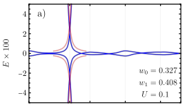
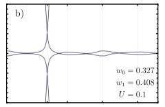
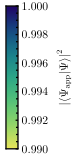
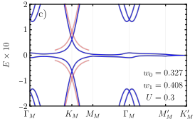
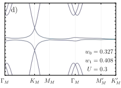
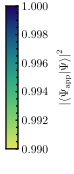
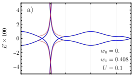
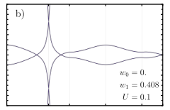
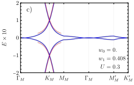
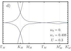
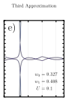
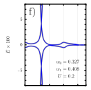
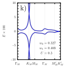
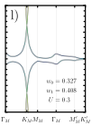
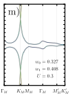
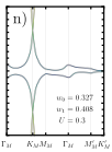
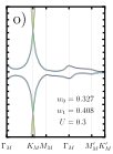
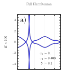
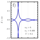
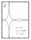
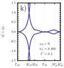
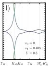
Figure 2: The low-energy band structure of TSTG in the presence of a perpendicular displacement field. The blue lines show the TSTG energy spectrum near charge neutrality for valley η=+\eta=+, computed by numerical diagonalization of the Hamiltonian in eq. 3 along high symmetry momentum lines. The tunneling parameters w0w_{0} and w1w_{1}, as well as the displacement field UU are specified inside each panel. Additionally, in panel (a) we illustrate schematically the four plane waves of the tripod model from eq. 25. We also highlight in yellow the A+1A_{+}^{1} region as defined in eq. 9, where the hybridization between the TBG active bands and the Dirac Hamiltonian is significant. The quantitative (qualitative) features of the TSTG band structure for U=0.1U=0.1 (U=0.3U=0.3) are accurately captured by the approximate dispersion of the tripod model in eq. 26, shown in red.

We now consider a simplified model for the low-energy physics of TSTG near the KMK_{M} point at 𝐤=𝐪1\mathbf{k}=\mathbf{q}_{1}. We employ the TBG tripod model Bistritzer and MacDonald 2011 that we further modify by coupling with a Dirac cone Hamiltonian, as required by eqs. 6 and 7. Focusing on the η=+\eta=+ valley and restricting to the four 𝐐\mathbf{Q}-points (i.e. four plane wave states) mandated by the tripod model (see fig. 2a), we write the single-particle eigenstates of TSTG as

|Ψ⁡(𝐤)⟩=∑α[∑i=03(ψi,α(𝐤)c^†𝐤,𝐐i,+,α,s)+ψD,α(𝐤)b^†𝐤,𝐐0,+,α,s]|0⟩,\begin{split}\ket{\Psi\left( \vec{k} \right)}=\sum_{\alpha}\left[\sum_{i=0}^{3}\left(\psi_{i,\alpha}\left(\mathbf{k}\right)\hat{c}^{\dagger}_{\mathbf{k},\mathbf{Q}_{i},+,\alpha,s}\right)\right.\\ +\left.\psi_{D,\alpha}\left(\mathbf{k}\right)\hat{b}^{\dagger}_{\mathbf{k},\mathbf{Q}_{0},+,\alpha,s}\right]\ket{0},\end{split} (23)

with 𝐐i=𝐪1+𝐪i\mathbf{Q}_{i}=\mathbf{q}_{1}+\mathbf{q}_{i} for i=1,2,3i=1,2,3 and 𝐐0=𝐪1\mathbf{Q}_{0}=\mathbf{q}_{1}. The first-quantized Hamiltonian acting on the ten-dimensional spinor

ΨT​(𝐤)=(ψ0T​(𝐤),ψ1T​(𝐤),ψ2T​(𝐤),ψ3T​(𝐤),ψDT​(𝐤))\Psi^{T}\hskip-3.00003pt\left(\mathbf{k}\right)=\left(\psi_{0}^{T}\left(\mathbf{k}\right),\psi_{1}^{T}\left(\mathbf{k}\right),\psi_{2}^{T}\left(\mathbf{k}\right),\psi_{3}^{T}\left(\mathbf{k}\right),\psi_{D}^{T}\left(\mathbf{k}\right)\right) (24)

is given by

HTri=(δ​𝐤⋅𝝈T1′T2′T3′U2​𝟙T1′h(1)​(δ​𝐤)𝟘𝟘𝟘T2′𝟘h(2)​(δ​𝐤)𝟘𝟘T3′𝟘𝟘h(3)​(δ​𝐤)𝟘U2​𝟙𝟘𝟘𝟘δ​𝐤⋅𝝈),H_{\mathrm{Tri}}=\begin{pmatrix}\delta\mathbf{k}\cdot\bm{\sigma}&T^{\prime}_{1}&T^{\prime}_{2}&T^{\prime}_{3}&\frac{U}{2}\mathbb{1}\\ T^{\prime}_{1}&h^{(1)}\left(\delta\mathbf{k}\right)&\mathbb{0}&\mathbb{0}&\mathbb{0}\\ T^{\prime}_{2}&\mathbb{0}&h^{(2)}\left(\delta\mathbf{k}\right)&\mathbb{0}&\mathbb{0}\\ T^{\prime}_{3}&\mathbb{0}&\mathbb{0}&h^{(3)}\left(\delta\mathbf{k}\right)&\mathbb{0}\\ \frac{U}{2}\mathbb{1}&\mathbb{0}&\mathbb{0}&\mathbb{0}&\delta\mathbf{k}\cdot\bm{\sigma}\end{pmatrix}, (25)

where we have introduced the shorthand notation h(i)​(δ​𝐤)=(δ​𝐤−𝐪i)⋅𝝈h^{(i)}\left(\delta\mathbf{k}\right)=\left(\delta\mathbf{k}-\mathbf{q}_{i}\right)\cdot\bm{\sigma} for i=1,2,3i=1,2,3 and δ​𝐤=𝐤−𝐪1\delta\mathbf{k}=\mathbf{k}-\mathbf{q}_{1}. In eq. 25, we have denoted the two-dimensional Pauli vector by 𝝈=(σx,σy)\bm{\sigma}=\left(\sigma_{x},\sigma_{y}\right) and defined the rescaled tunneling matrices Ti′=Ti​2T^{\prime}_{i}=T_{i}\sqrt{2} (for i=1,2,3i=1,2,3), with TiT_{i} being given in eq. 82. The 10×1010\times 10 Hamiltonian matrix in eq. 25 cannot be solved analytically. However, we are interested in the low-energy physics of TSTG near the KMK_{M} point, for which δ​k∼E≪1\delta k\sim E\ll 1 (where δ​k=|δ​𝐤|\delta k=\absolutevalue{\delta\vec{k}} and EE is the energy of the state at δ​𝐤\delta\mathbf{k}), as can be seen in fig. 2. Thanks to a series of justified approximations detailed in Appendix D.1, we can analytically obtain the low-energy dispersion relation near KMK_{M}

E=±δ​k​(3​w0′2+2)±9​δ​k2​(w0′2+2​w1′2)2+U2​Δ2​Δ,E=\pm\frac{\delta k\left(3w_{0}^{\prime 2}+2\right)\pm\sqrt{9\delta k^{2}\left(w_{0}^{\prime 2}+2w_{1}^{\prime 2}\right)^{2}+U^{2}\Delta}}{2\Delta}, (26)

where Δ=(3​w0′2+3​w1′2+1)\Delta=\left(3w_{0}^{\prime 2}+3w_{1}^{\prime 2}+1\right) and w0,1′=w0,1​2w^{\prime}_{0,1}=w_{0,1}\sqrt{2}. We plot the approximate dispersion relation of eq. 26 in fig. 2: the simplified tripod model qualitatively and quantitatively matches the low-energy spectrum of H^0\hat{H}_{0} obtained from numerical diagonalization with a large number of 𝐐\mathbf{Q} points. Note that a similar tripod model was derived in Ref. Li et al. 2019 but only for U=0U=0.

IV.3 The low-energy spectrum of TSTG

The low-energy physics of TSTG with displacement field arises from the interplay between the almost-flat bands of H^TBG\hat{H}_{\mathrm{TBG}} and the Dirac cone bands of H^D\hat{H}_{D} with which they are coupled by H^U\hat{H}_{U}. We are interested in a quantitative perturbation theory for the single-particle wave functions of TSTG in the presence of a non-zero displacement field. Ideally, we would also like to express the low-energy eigenstates of H^0\hat{H}_{0} only in terms of the eigenstates of H^TBG\hat{H}_{\mathrm{TBG}}: while they cannot be analytically computed in the entire MBZ, their properties have been extensively studied in Refs. Song et al. 2019; Bernevig et al. 2020a; Bernevig et al. 2020b; Song et al. 2020.

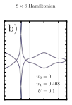
In Appendix D.2, we show that rather than starting from the full TSTG Hamiltonian in eq. 3 and then projecting into its low energy states, an excellent approximation is to start from the TBG Hamiltonian projected into the active bands (HTBGH_{\mathrm{TBG}}) which is then hybridized with the Dirac cone fermions. For valley η=+\eta=+ (η=−\eta=-), the Hamiltonian HTBG+H^D+H^UH_{\mathrm{TBG}}+\hat{H}_{D}+\hat{H}_{U} leads to close to the exact (i.e. with an overlap higher than 99%99\%) eigenstates around the KMK_{M} (KM′K_{M}^{\prime}) point within a radius Λ\Lambda for both the active and the Dirac cone bands. It also captures the correct eigenstates at ΓM\Gamma_{M} for the active TBG bands, which are not changed much by the introduction of the displacement field. Note that around ΓM\Gamma_{M}, this method will not give the correct eigenstates for the Dirac cone bands (which are, however, at high energy and do not contribute to the low-energy physics). Indeed, the high Fermi velocity of the Dirac cone bands implies that they hybridize with the higher energy (passive) bands of H^TBG\hat{H}_{\mathrm{TBG}} that we neglect in the projection (see fig. 2).

Using only three plane wave states (i.e. three 𝐐\mathbf{Q} points) for the mirror-antisymmetric fermions (an approximation which was justified numerically in Appendix A.1), we can write the low-energy single-particle eigenstates of H^0\hat{H}_{0} for valley η\eta, spin ss, and band labeled by mm as

|Ψη,s,m​(𝐤)⟩=[∑i=13∑α(ψη,s,mi,α(𝐤)b^†𝐤,η​𝐪i,η,α,s)+∑|n|=1ϕη,s,mn(𝐤)c^†𝐤,n,η,s]|0⟩,\begin{split}\ket{\Psi^{\eta,s,m} \left( \vec{k} \right)}=\left[\sum_{i=1}^{3}\sum_{\alpha}\left(\psi^{\eta,s,m}_{i,\alpha}\left(\mathbf{k}\right)\hat{b}^{\dagger}_{\mathbf{k},\eta\mathbf{q}_{i},\eta,\alpha,s}\right)\right.\\ \left.+\sum_{\absolutevalue{n}=1}\phi^{\eta,s,m}_{n}\left(\mathbf{k}\right)\hat{c}^{\dagger}_{\mathbf{k},n,\eta,s}\right]\ket{0},\end{split} (27)

where we have defined the three two-component spinors on the sublattice space, ψiη,s,m​(𝐤)\psi^{\eta,s,m}_{i}\left(\mathbf{k}\right) (for i=1,2,3i=1,2,3), and the two-component spinor in the space of the n=±1n=\pm 1 TBG active bands, ϕη,s,m​(𝐤)\phi^{\eta,s,m}\left(\mathbf{k}\right). When acting on the eight-dimensional spinor

ΨT​(𝐤)=(ψ1T​(𝐤),ψ2T​(𝐤),ψ3T​(𝐤),ϕT​(𝐤)),\Psi^{T}\left(\mathbf{k}\right)=\left(\psi^{T}_{1}\left(\mathbf{k}\right),\psi^{T}_{2}\left(\mathbf{k}\right),\psi^{T}_{3}\left(\mathbf{k}\right),\phi^{T}\left(\mathbf{k}\right)\right), (28)

we obtain the following analytical expression for the low-energy the 8×88\times 8 first-quantized TSTG Hamiltonian

H8×8=(ℰηU1†η​(𝐤)U2†η​(𝐤)U3†η​(𝐤)U1η​(𝐤)hη​𝐪𝟏D,η​(𝐤)𝟘𝟘U2η​(𝐤)𝟘hη​𝐪𝟐D,η​(𝐤)𝟘U3η​(𝐤)𝟘𝟘hη​𝐪𝟑D,η​(𝐤)).H_{8\times 8}=\begin{pmatrix}\mathcal{E}^{\eta}&U^{\dagger\eta}_{1}\left(\mathbf{k}\right)&U^{\dagger\eta}_{2}\left(\mathbf{k}\right)&U^{\dagger\eta}_{3}\left(\mathbf{k}\right)\\ U^{\eta}_{1}\left(\mathbf{k}\right)&h^{D,\eta}_{\mathbf{\eta\mathbf{q}_{1}}}\left(\mathbf{k}\right)&\mathbb{0}&\mathbb{0}\\ U^{\eta}_{2}\left(\mathbf{k}\right)&\mathbb{0}&h^{D,\eta}_{\mathbf{\eta\mathbf{q}_{2}}}\left(\mathbf{k}\right)&\mathbb{0}\\ U^{\eta}_{3}\left(\mathbf{k}\right)&\mathbb{0}&\mathbb{0}&h^{D,\eta}_{\mathbf{\eta\mathbf{q}_{3}}}\left(\mathbf{k}\right)\end{pmatrix}. (29)

For the sake of brevity, in eq. 28, we have suppressed the η\eta, ss, and mm indices. In addition, in eq. 29 the 2×22\times 2 diagonal energy matrix for the TBG active bands in valley η\eta is given by

ℰη​(𝐤)=(ϵ+1,ηc^​(𝐤)00ϵ−1,ηc^​(𝐤))\mathcal{E}^{\eta}\left(\mathbf{k}\right)=\begin{pmatrix}\epsilon^{\hat{c}}_{+1,\eta}\left(\mathbf{k}\right)&0\\ 0&\epsilon^{\hat{c}}_{-1,\eta}\left(\mathbf{k}\right)\\ \end{pmatrix} (30)

whereas the 2×22\times 2 displacement field perturbation matrices can be written in terms of the TBG wave functions defined in eq. 20

[Uiη​(𝐤)]α,n=U2​uη​𝐪i​α;n​ηc^​(𝐤),\left[U^{\eta}_{i}\left(\mathbf{k}\right)\right]_{\alpha,n}=\frac{U}{2}u^{\hat{c}}_{\eta\mathbf{q}_{i}\alpha;n\eta}\left(\mathbf{k}\right), (31)

for i=1,2,3i=1,2,3. As anticipated in section II.3, there are two regions of interest in the BZ for the low-energy spectrum of H0H_{0} and hence of H8×8H_{8\times 8}: away and near the Dirac points of the MBZ. In deriving the single-particle projected TSTG Hamiltonian, we will now consider each of them individually.

IV.4 Single-particle projected TSTG Hamiltonian

We first provide the final expression of the single-particle projected TSTG Hamiltonian. We then sketch its derivation, with the detailed proof given in Appendix D.2. The single-particle projected TSTG Hamiltonian reads

H0=HTBG+HD+HU(b^​c^)+HU(c^),H_{0}=H_{\mathrm{TBG}}+H_{D}+H^{\left(\hat{b}\hat{c}\right)}_{U}+H^{\left(\hat{c}\right)}_{U}, (32)

where we have introduced the single-particle projected TBG Bernevig et al. 2020b and Dirac Hamiltonians, which are respectively given by

HTBG\displaystyle H_{\mathrm{TBG}} =∑|n|=1η,s𝐤∈MBZϵn,ηc^​(𝐤)​c^𝐤,n,η,s†​c^𝐤,n,η,s,\displaystyle=\sum_{\begin{subarray}{c}\absolutevalue{n}=1\\ \eta,s\\ \mathbf{k}\in\mathrm{MBZ}\end{subarray}}\epsilon_{n,\eta}^{\hat{c}}\left(\mathbf{k}\right)\hat{c}^{\dagger}_{\mathbf{k},n,\eta,s}\hat{c}_{\mathbf{k},n,\eta,s}, (33)
HD\displaystyle H_{D} =∑|n|=1η,s|δ​𝐤|≤Λϵn,ηb^​(δ​𝐤)​b^δ​𝐤+η​𝐪1,n,η,s†​b^δ​𝐤+η​𝐪1,n,η,s.\displaystyle=\sum_{\begin{subarray}{c}\absolutevalue{n}=1\\ \eta,s\\ \absolutevalue{\delta\vec{k}}\leq\Lambda\end{subarray}}\epsilon_{n,\eta}^{\hat{b}}\left(\delta\mathbf{k}\right)\hat{b}^{\dagger}_{\delta\mathbf{k}+\eta\mathbf{q}_{1},n,\eta,s}\hat{b}_{\delta\mathbf{k}+\eta\mathbf{q}_{1},n,\eta,s}. (34)

Note that HDH_{D} is only defined on a small region (|δ​𝐤|≤Λ≤0.2\absolutevalue{ \delta\vec{k} }\leq\Lambda\leq 0.2) of the MBZ as a consequence of the high Fermi velocity of the Dirac cone bands for which

ϵ±1,ηb^​(δ​𝐤)=±|δ​𝐤|.\epsilon_{\pm 1,\eta}^{\hat{b}}\left(\delta\mathbf{k}\right)=\pm\absolutevalue{\delta\vec{k}}. (35)

Equation 32 also incorporates the effects of a non-zero displacement field through the contributions HU(b^​c^)H^{\left(\hat{b}\hat{c}\right)}_{U} (mixing the TBG and Dirac bands) and HU(c^)H^{\left(\hat{c}\right)}_{U} (mixing the two active TBG bands within each valley and spin). These last two terms in eq. 32 capture the effects of the perpendicular displacement field in the two regions of the MBZ and will be derived below.

IV.4.1 Perturbation theory away from the Dirac points

Away from the Dirac points, i.e. when 𝐤∈𝒞η\mathbf{k}\in\mathcal{C}_{\eta}, where

𝒞η=(MBZ∖⋃i=13Aηi),\mathcal{C}_{\eta}=\left(\mathrm{MBZ}\setminus\bigcup_{i=1}^{3}A_{\eta}^{i}\right), (36)

the hybridization between the eigenstates of H^D\hat{H}_{D} and the active bands of H^TBG\hat{H}_{\mathrm{TBG}} is suppressed by the difference in their energies. We can eliminate the ψi\psi_{i} spinors of eq. 29 by writing them in terms of ϕ\phi

ψi=(E−hi)−1​Ui​ϕ,\psi_{i}=\left(E-h_{i}\right)^{-1}U_{i}\phi, (37)

where we have suppressed the valley indices and made the 𝐤\mathbf{k}-dependence implicit. In addition we have also introduced the shorthand notation hi≡hη​𝐪iD,η​(𝐤)h_{i}\equiv h_{\eta\mathbf{q}_{i}}^{D,\eta}\left(\mathbf{k}\right). Equation 29 can thus be cast as a non-linear eigenvalue equation

[ℰ+∑i=13Ui†​(E−hi)−1​Ui]​ϕ=E​ϕ.\left[\mathcal{E}+\sum_{i=1}^{3}U^{\dagger}_{i}\left(E-h_{i}\right)^{-1}U_{i}\right]\phi=E\phi. (38)

We expect the energy of the active bands to be only slightly changed by the hybridization with the Dirac cone Hamiltonian in the region 𝒞η\mathcal{C}_{\eta} and have |E|≪|hi|=|𝐤−η​𝐪i|\absolutevalue{E}\ll\absolutevalue{h_i}=\absolutevalue{\vec{k} - \eta\vec{q}_i}. We can therefore ignore the EE dependence in the denominator of the second term of eq. 38 11 1 Alternatively, we can expand (E−hi)−1\left(E-h_{i}\right)^{-1} to linear order in EE, and still end up with an analytically solvable equation. In this paper, we will ignore this linear contribution.. This affords a major simplification as the Hamiltonians hih_{i} can be readily inverted to give a linear eigenvalue equation

[ℰ+∑i=13Ui†​hi−1​Ui]​ϕ=E​ϕ.\left[\mathcal{E}+\sum_{i=1}^{3}U^{\dagger}_{i}h_{i}^{-1}U_{i}\right]\phi=E\phi. (39)

We show in Appendix D.2.2 that the amplitude of the mirror-antisymmetric operators is small enough in this region, validating an approximation even at large values of UU: for 𝐤∈𝒞η\mathbf{k}\in\mathcal{C}_{\eta}, the displacement field only induces mixing between the active TBG bands. This contribution is captured by the effective Hamiltonian

HU(c^)=∑|n|,|m|=1η,s∑𝐤∈𝒞ηℬn​mη​(𝐤)​c^𝐤,n,η,s†​c^𝐤,m,η,s,H^{\left(\hat{c}\right)}_{U}=\sum_{\begin{subarray}{c}\absolutevalue{n},\absolutevalue{m}=1\\ \eta,s\end{subarray}}\sum_{\begin{subarray}{c}\mathbf{k}\in\mathcal{C}_{\eta}\end{subarray}}\mathcal{B}^{\eta}_{nm}\left(\mathbf{k}\right)\hat{c}^{\dagger}_{\mathbf{k},n,\eta,s}\hat{c}_{\mathbf{k},m,\eta,s}, (40)

where the matrix ℬn​mη\mathcal{B}^{\eta}_{nm} is given in eq. 186 of Appendix D.2.2 and represents a second-order contribution in UU. For small enough displacement fields (i.e. when U2/|𝐤−η​𝐪i|U^{2}/\absolutevalue{\vec{k} - \eta\vec{q}_i} is much smaller than the bandwidth of the TBG flat bands), the active band states will not be significantly perturbed.

IV.4.2 Perturbation theory near the Dirac points

Near any of the three Dirac points in the MBZ, the mixing between the TBG active bands and the Dirac cone Hamiltonian is significant. If 𝐤\mathbf{k} is near the jj-th Dirac point in the MBZ (i.e. 𝐤∈Aηj\mathbf{k}\in A_{\eta}^{j}), we will have |hj|≪1\absolutevalue{h_j}\ll 1, but |hi|≈3\absolutevalue{h_i}\approx\sqrt{3}, for i≠ji\neq j. This implies that while the hybridization between the TBG active bands and the jj-th Dirac Hamiltonian is relevant, there is little to no mixing with the Dirac cone bands stemming from the other two Dirac points of H^D\hat{H}_{D} in the MBZ. We can therefore approximate ψi≈0\psi_{i}\approx 0 for i≠ji\neq j and write the single-particle TSTG wave functions for 𝐤∈Aηj\mathbf{k}\in A_{\eta}^{j} as

|Ψη,s,m​(𝐤)⟩=[∑α(ψη,s,mj,α(𝐤)b^†𝐤,η​𝐪j,η,α,s)+∑|n|=1ϕη,s,mn(𝐤)c^†𝐤,n,η,s]|0⟩.\begin{split}\ket{\Psi^{\eta,s,m} \left( \vec{k} \right)}=\left[\sum_{\alpha}\left(\psi^{\eta,s,m}_{j,\alpha}\left(\mathbf{k}\right)\hat{b}^{\dagger}_{\mathbf{k},\eta\mathbf{q}_{j},\eta,\alpha,s}\right)+\right.\\ \left.\sum_{\absolutevalue{n}=1}\phi^{\eta,s,m}_{n}\left(\mathbf{k}\right)\hat{c}^{\dagger}_{\mathbf{k},n,\eta,s}\right]\ket{0}.\end{split} (41)

In this region all four bands arising from the hybridization between the TBG active bands and the Dirac cone Hamiltonian are relevant for the low energy of TSTG. The corresponding first-quantized Hamiltonian reads

H4×4=(ℰη​(𝐤)Uj†η​(𝐤)Ujη​(𝐤)hη​𝐪jD,η​(𝐤)).H_{4\times 4}=\begin{pmatrix}\mathcal{E}^{\eta}\left(\mathbf{k}\right)&U^{\dagger\eta}_{j}\left(\mathbf{k}\right)\\ U^{\eta}_{j}\left(\mathbf{k}\right)&h^{D,\eta}_{\eta\mathbf{q}_{j}}\left(\mathbf{k}\right)\end{pmatrix}. (42)

In Appendix D.2.3, we present a series of approximations which renders this 4×44\times 4 Hamiltonian exactly solvable in the (first) chiral limit. In the general case, we will write the projected displacement field Hamiltonian in this region of the MBZ in the energy band basis as

HU(b^​c^)=∑η,s|n|,|m|=1|δ​𝐤|≤Λ[Nm​nη(δ𝐤)b^𝐤η,m,η,s†c^𝐤η,n,η,s+h.c.],H^{\left(\hat{b}\hat{c}\right)}_{U}\hskip-3.99994pt=\hskip-10.00002pt\sum_{\begin{subarray}{c}\eta,s\\ \absolutevalue{n},\absolutevalue{m}=1\\ \absolutevalue{\delta\vec{k}}\leq\Lambda\end{subarray}}\hskip-11.00008pt\left[N^{\eta}_{mn}\left(\delta\mathbf{k}\right)\hat{b}^{\dagger}_{\mathbf{k}_{\eta},m,\eta,s}\hat{c}_{\mathbf{k}_{\eta},n,\eta,s}+\mathrm{h.c.}\right], (43)

where 𝐤η≡δ​𝐤+η​𝐪1\mathbf{k}_{\eta}\equiv\delta\mathbf{k}+\eta\mathbf{q}_{1} and the displacement field overlap matrix Nm​nηN^{\eta}_{mn} is defined in eq. 200 of Appendix D.2.3.

V Many-body TSTG Hamiltonian

This section introduces the interacting Hamiltonian for TSTG. We only quote the main results here; the complete derivations are relegated to Appendix F. We start by writing the Coulomb repulsion Hamiltonian in terms of the moiré lattice fermion operators introduced in section II. Next, we show how the expression of the interaction Hamiltonian can be simplified by employing fermion operators corresponding to each mirror-symmetry sector. Using the energy band bases for the TBG and Dirac single-particle Hamiltonians defined in section IV.1, we project the interaction Hamiltonian in the low-energy TSTG eigenstates. Finally, we write the expression for the fully-interacting TSTG Hamiltonian which is shown to have a spatial many-body charge-conjugation symmetry.

V.1 Coulomb interaction in TSTG

The (unprojected) low-energy interaction Hamiltonian governing electron-electron repulsion in TSTG reads

H^I=12​Ωtot​∑𝐆∈𝒬0𝐪∈MBZl,l′Vl,l′​(𝐪+𝐆)​δ​ρ𝐆+𝐪l​δ​ρ−𝐆−𝐪l′,\hat{H}_{I}=\frac{1}{2\Omega_{\mathrm{tot}}}\sum_{\begin{subarray}{c}\mathbf{G}\in\mathcal{Q}_{0}\\ \mathbf{q}\in\mathrm{MBZ}\\ l,l^{\prime}\end{subarray}}V^{l,l^{\prime}}\left(\mathbf{q}+\mathbf{G}\right)\delta\rho^{l}_{\mathbf{G}+\mathbf{q}}\delta\rho^{l^{\prime}}_{-\mathbf{G}-\mathbf{q}}, (44)

where Ωtot\Omega_{\mathrm{tot}} is the total area of the TSTG sample and we have defined the Fourier transformation of the relative (to the single-layer graphene charge neutral point) electron density operators corresponding to layer ll to be

δ​ρ𝐆+𝐪l=∑η,α,s∑𝐤∈MBZ𝐐∈𝒬η,l(a^𝐤,𝐐,η,α,s,l†​a^𝐤−𝐪,𝐆+𝐐,η,α,s,lCLOSEOPEN−12​δ𝐪,𝟎​δ𝐆,𝟎).\begin{split}\delta\rho^{l}_{\mathbf{G}+\mathbf{q}}=\sum_{\eta,\alpha,s}\sum_{\begin{subarray}{c}\mathbf{k}\in\mathrm{MBZ}\\ \mathbf{Q}\in\mathcal{Q}_{\eta,l}\end{subarray}}\left(\hat{a}^{\dagger}_{\mathbf{k},\mathbf{Q},\eta,\alpha,s,l}\hat{a}_{\mathbf{k}-\mathbf{q},\mathbf{G}+\mathbf{Q},\eta,\alpha,s,l}\right.\\ \left.-\frac{1}{2}\delta_{\mathbf{q},\mathbf{0}}\delta_{\mathbf{G},\mathbf{0}}\right).\end{split} (45)

In eq. 44, Vl,l′​(𝐪+𝐆)V^{l,l^{\prime}}\left(\mathbf{q}+\mathbf{G}\right) represents the Fourier transformation of the screened Coulomb potential Vl,l′​(𝐫)V^{l,l^{\prime}}\left(\mathbf{r}\right) governing the repulsion between two electrons located respectively in layers ll and l′l^{\prime} and separated by a distance 𝐫\mathbf{r}, measured in the plane of the single layer graphene. In the definition of the relative density operators from eq. 45, we are effectively ignoring the inter-valley scattering processes, which are suppressed by the decay of the Coulomb potential in momentum space on a scale much smaller than the inter-valley separation of single layer graphene (see Appendix F.1.1).

For the typical gated arrangement used in experiments Hao et al. 2021; Park et al. 2021, the interlayer distance (typically 3 Å3\text{\,}\mathrm{\SIUnitSymbolAngstrom}) in TSTG is much smaller than the gate separation ξ\xi (usually 10 nm10\text{\,}\mathrm{nm}) enabling us to neglect the dependence of Vl,l′​(𝐪+𝐆)V^{l,l^{\prime}}\left(\mathbf{q}+\mathbf{G}\right) on the layer indices ll and l′l^{\prime} (see Appendix F.1.2) and write the screened Coulomb interaction as

Vl,l′​(𝐪)≈V⁡(𝐪)=2​π​e2ϵ​tanh⁡(ξ​|𝐪|/2)|𝐪|.V^{l,l^{\prime}}\left(\mathbf{q}\right)\approx V\left(\mathbf{q}\right)=\frac{2\pi e^{2}}{\epsilon}\frac{\tanh\left(\xi\absolutevalue{\vec{q}}/2\right)}{\absolutevalue{\vec{q}}}. (46)

This allows for a significant simplification, since the interaction Hamiltonian can now be written in terms of the relative density operators corresponding to the two mirror-symmetry sectors

δ​ρ𝐆+𝐪c^=∑𝐤∈MBZ𝐐∈𝒬±η,α,s(c^𝐤,𝐐,η,α,s†​c^𝐤−𝐪,𝐆+𝐐,η,α,s−12​δ𝐪,𝟎​δ𝐆,𝟎),δ​ρ𝐆+𝐪b^=∑𝐤∈MBZ𝐐∈𝒬ηη,α,s(b^𝐤,𝐐,η,α,s†​b^𝐤−𝐪,𝐆+𝐐,η,α,s−12​δ𝐪,𝟎​δ𝐆,𝟎),\begin{split}\delta\rho^{\hat{c}}_{\mathbf{G}+\mathbf{q}}&=\sum_{\begin{subarray}{c}\mathbf{k}\in\mathrm{MBZ}\\ \mathbf{Q}\in\mathcal{Q}_{\pm}\\ \eta,\alpha,s\end{subarray}}\left(\hat{c}^{\dagger}_{\mathbf{k},\mathbf{Q},\eta,\alpha,s}\hat{c}_{\mathbf{k}-\mathbf{q},\mathbf{G}+\mathbf{Q},\eta,\alpha,s}-\frac{1}{2}\delta_{\mathbf{q},\mathbf{0}}\delta_{\mathbf{G},\mathbf{0}}\right),\\ \delta\rho^{\hat{b}}_{\mathbf{G}+\mathbf{q}}&=\sum_{\begin{subarray}{c}\mathbf{k}\in\mathrm{MBZ}\\ \mathbf{Q}\in\mathcal{Q}_{\eta}\\ \eta,\alpha,s\end{subarray}}\left(\hat{b}^{\dagger}_{\mathbf{k},\mathbf{Q},\eta,\alpha,s}\hat{b}_{\mathbf{k}-\mathbf{q},\mathbf{G}+\mathbf{Q},\eta,\alpha,s}-\frac{1}{2}\delta_{\mathbf{q},\mathbf{0}}\delta_{\mathbf{G},\mathbf{0}}\right),\end{split} (47)

We can thus separate the interaction Hamiltonian from eq. 44 into three contributions

H^I=H^I,TBG+H^I,D+H^I,TBG−D.\hat{H}_{I}=\hat{H}_{I,\mathrm{TBG}}+\hat{H}_{I,D}+\hat{H}_{I,\mathrm{TBG}-D}. (48)

The first and second terms in eq. 48 respectively represent the interaction Hamiltonians for ordinary TBG and for Dirac cone fermions

H^I,TBG\displaystyle\hat{H}_{I,\mathrm{TBG}} =12​Ωtot​∑𝐪∈MBZ𝐆∈𝒬0V⁡(𝐪+𝐆)​δ​ρ𝐆+𝐪c^​δ​ρ−𝐆−𝐪c^,\displaystyle=\frac{1}{2\Omega_{\mathrm{tot}}}\sum_{\begin{subarray}{c}\mathbf{q}\in\mathrm{MBZ}\\ \mathbf{G}\in\mathcal{Q}_{0}\end{subarray}}V\left(\mathbf{q}+\mathbf{G}\right)\delta\rho^{\hat{c}}_{\mathbf{G}+\mathbf{q}}\delta\rho^{\hat{c}}_{-\mathbf{G}-\mathbf{q}}, (49)
H^I,D\displaystyle\hat{H}_{I,D} =12​Ωtot​∑𝐪∈MBZ𝐆∈𝒬0V⁡(𝐪+𝐆)​δ​ρ𝐆+𝐪b^​δ​ρ−𝐆−𝐪b^.\displaystyle=\frac{1}{2\Omega_{\mathrm{tot}}}\sum_{\begin{subarray}{c}\mathbf{q}\in\mathrm{MBZ}\\ \mathbf{G}\in\mathcal{Q}_{0}\end{subarray}}V\left(\mathbf{q}+\mathbf{G}\right)\delta\rho^{\hat{b}}_{\mathbf{G}+\mathbf{q}}\delta\rho^{\hat{b}}_{-\mathbf{G}-\mathbf{q}}. (50)

The third term corresponds to the Coulomb interaction between the TBG and Dirac cone fermions

H^I,TBG−D=12​Ωtot​∑𝐪∈MBZ𝐆∈𝒬0V⁡(𝐪+𝐆)×[δρc^𝐆+𝐪δρb^−𝐆−𝐪+h.c.].\begin{split}\hat{H}_{I,\mathrm{TBG}-D}=\frac{1}{2\Omega_{\mathrm{tot}}}\sum_{\begin{subarray}{c}\mathbf{q}\in\mathrm{MBZ}\\ \mathbf{G}\in\mathcal{Q}_{0}\end{subarray}}V\left(\mathbf{q}+\mathbf{G}\right)\\ \times\left[\delta\rho^{\hat{c}}_{\mathbf{G}+\mathbf{q}}\delta\rho^{\hat{b}}_{-\mathbf{G}-\mathbf{q}}+\mathrm{h.c.}\right].\end{split} (51)

Notice that the decomposition in eq. 48 is valid even when the mzm_{z} symmetry is broken in the presence of a perpendicular displacement field U≠0U\neq 0.

V.2 Interaction projected Hamiltonian

Having derived the interaction Hamiltonian in the TSTG mirror-symmetry basis defined in eqs. 1 and 2, we now turn our attention to projecting it in the low-energy TSTG single-particle eigenstates. As shown in Appendix F.2, the projected interaction Hamiltonian (henceforth denoted without a hat) reads

HI=12​Ωtot​∑𝐆∈𝒬0𝐪∈MBZ(O𝐪,𝐆c^+O𝐪,𝐆b^)†​(O𝐪,𝐆c^+O𝐪,𝐆b^)H_{I}=\frac{1}{2\Omega_{\mathrm{tot}}}\hskip-5.0pt\sum_{\begin{subarray}{c}\mathbf{G}\in\mathcal{Q}_{0}\\ \mathbf{q}\in\mathrm{MBZ}\end{subarray}}\hskip-5.0pt\left(O^{\hat{c}}_{\mathbf{q},\mathbf{G}}+O^{\hat{b}}_{\mathbf{q},\mathbf{G}}\right)^{\dagger}\left(O^{\hat{c}}_{\mathbf{q},\mathbf{G}}+O^{\hat{b}}_{\mathbf{q},\mathbf{G}}\right) (52)

where we have introduced the operators

O𝐪,𝐆c^=V⁡(𝐪+𝐆)​∑𝐤∈MBZ|n|,|m|=1η,sMm​nc^,η​(𝐤,𝐪+𝐆)×(c^𝐤+𝐪,m,η,s†​c^𝐤,n,η,s−12​δ𝐪,𝟎​δm,n).\begin{split}O^{\hat{c}}_{\mathbf{q},\mathbf{G}}=\sqrt{V\left(\mathbf{q}+\mathbf{G}\right)}\sum_{\begin{subarray}{c}\mathbf{k}\in\mathrm{MBZ}\\ \absolutevalue{n},\absolutevalue{m}=1\\ \eta,s\end{subarray}}M^{\hat{c},\eta}_{mn}\left(\mathbf{k},\mathbf{q}+\mathbf{G}\right)\\ \times\left(\hat{c}^{\dagger}_{\mathbf{k}+\mathbf{q},m,\eta,s}\hat{c}_{\mathbf{k},n,\eta,s}-\frac{1}{2}\delta_{\mathbf{q},\mathbf{0}}\delta_{m,n}\right).\end{split} (53)

and

O𝐪,𝐆b^=V⁡(𝐪+𝐆)​∑|δ​𝐤|,|δ​𝐤+𝐪|≤Λ|n|,|m|=1η,sMm​nb^,η​(𝐤η,𝐪+𝐆)×(b^𝐤η+𝐪,m,η,s†​b^𝐤η,n,η,s−12​δ𝐪,𝟎​δm,n),\begin{split}O^{\hat{b}}_{\mathbf{q},\mathbf{G}}=\sqrt{V\left(\mathbf{q}+\mathbf{G}\right)}\sum_{\begin{subarray}{c}\absolutevalue{\delta\vec{k}},\absolutevalue{\delta\vec{k} + \vec{q}}\leq\Lambda\\ \absolutevalue{n},\absolutevalue{m}=1\\ \eta,s\end{subarray}}\hskip-10.00002ptM^{\hat{b},\eta}_{mn}\left(\mathbf{k}_{\eta},\mathbf{q}+\mathbf{G}\right)\\ \times\left(\hat{b}^{\dagger}_{\mathbf{k}_{\eta}+\mathbf{q},m,\eta,s}\hat{b}_{\mathbf{k}_{\eta},n,\eta,s}-\frac{1}{2}\delta_{\mathbf{q},\mathbf{0}}\delta_{m,n}\right),\end{split} (54)

with 𝐤η≡δ​𝐤+𝐪1\mathbf{k}_{\eta}\equiv\delta\mathbf{k}+\mathbf{q}_{1}. Note that the expression of O𝐪,𝐆c^O^{\hat{c}}_{\mathbf{q},\mathbf{G}} is identical to the one corresponding to ordinary TBG derived in Ref. Bernevig et al. 2020b. Additionally, the operators O𝐪,𝐆f^O^{\hat{f}}_{\mathbf{q},\mathbf{G}} commute with each other, i.e. [O𝐪1,𝐆1b^,O𝐪2,𝐆2c^]=0\left[O^{\hat{b}}_{\mathbf{q}_{1},\mathbf{G}_{1}},O^{\hat{c}}_{\mathbf{q}_{2},\mathbf{G}_{2}}\right]=0, and obey O−𝐪,−𝐆f^=O𝐪,𝐆†f^O^{\hat{f}}_{-\mathbf{q},-\mathbf{G}}=O^{\dagger\hat{f}}_{\mathbf{q},\mathbf{G}}, for f^=c^,b^\hat{f}=\hat{c},\hat{b}. In eqs. 53 and 54, the form factors Mm​nc^,ηM^{\hat{c},\eta}_{mn} and Mm​nb^,ηM^{\hat{b},\eta}_{mn} are defined in terms of the single-particle TBG and Dirac cone single-particle wave functions introduced in section IV.1 as

Mm​nf^,η​(𝐤,𝐪+𝐆)=∑α𝐐∈𝒬±u𝐐−𝐆​α;m​η∗f^​(𝐤+𝐪)​u𝐐​α;n​ηf^​(𝐤),M^{\hat{f},\eta}_{mn}\left(\mathbf{k},\mathbf{q}+\mathbf{G}\right)=\sum_{\begin{subarray}{c}\alpha\\ \mathbf{Q}\in\mathcal{Q}_{\pm}\end{subarray}}u^{*\hat{f}}_{\mathbf{Q}-\mathbf{G}\alpha;m\eta}\left(\mathbf{k}+\mathbf{q}\right)u^{\hat{f}}_{\mathbf{Q}\alpha;n\eta}\left(\mathbf{k}\right), (55)

for f^=c^,b^\hat{f}=\hat{c},\hat{b}.

For the mirror-symmetric operators, the projection in the TSTG low-energy modes is equivalent to restricting the summation in eq. 53 to the active TBG bands. For the Dirac cone fermions, we additionally restrict the momenta in eq. 54 to lie near the Dirac points of HDH_{D} located at η​𝐪1\eta\mathbf{q}_{1} for valley η\eta. The TBG form-factors Mm​nc^,η​(𝐤,𝐪+𝐆)M^{\hat{c},\eta}_{mn}\left(\mathbf{k},\mathbf{q}+\mathbf{G}\right) were shown to decay exponentially with |𝐆|\absolutevalue{\vec{G}} Bernevig et al. 2020a. As such, only a few moiré reciprocal vectors 𝐆\mathbf{G} contribute to the summation in eq. 52: the reciprocal vectors 𝐆\mathbf{G} for which |𝐆|=0,3\absolutevalue{\vec{G}}=0,\sqrt{3}. On the other hand, the Dirac cone form factors Mm​nb^,η​(𝐤,𝐪+𝐆)M^{\hat{b},\eta}_{mn}\left(\mathbf{k},\mathbf{q}+\mathbf{G}\right) vanish completely for any non-zero reciprocal vector 𝐆\mathbf{G}, provided that the cutoff Λ\Lambda is small enough (as shown in Appendix F.2).

Finally, we note that the projected interaction Hamiltonian in eq. 52 is a sum of positive semidefinite operators, and hence is itself positive semidefinite Kang and Vafek 2019, similarly to the case of TBG Bultinck et al. 2020a; Bernevig et al. 2020b.

V.3 Many-body projected TSTG Hamiltonian

The expression of the interaction projected TSTG Hamiltonian eq. 52 can finally be combined with the projected single-particle Hamiltonian from eq. 32 to yield the many-body projected TSTG Hamiltonian

H=H0+HI.H=H_{0}+H_{I}. (56)

Investigating the symmetries of HH under various different limits forms the object of section VI. For now, we will only mention that HH features a spatial many-body charge conjugation symmetry 𝒫\mathcal{P} defined by the action of the single-particle anti-unitary transformation

𝒰=mz​C2​x​C2​z​T​P\mathcal{U}=m_{z}C_{2x}C_{2z}TP (57)

followed by the interchange of the creation and annihilation fermion operators (see Appendix G.1 for details). The many-body projected Hamiltonian HH is invariant under the action of 𝒫\mathcal{P}, i.e.

𝒫​H​𝒫−1=H\mathcal{P}H\mathcal{P}^{-1}=H (58)

In particular, 𝒫\mathcal{P} maps a many-body state with NeN_{e} electrons to a state with −Ne-N_{e} electrons, where number of electrons is measured with respect to the TSTG charge neutral point. As a consequence of the charge conjugation symmetry 𝒫\mathcal{P}, the eigenspectrum of the fully-interacting projected TSTG Hamiltonian is symmetric about the charge neutral point.

Finally, we note that the projected interaction Hamiltonian from eq. 52 is not normal ordered. The difference between HIH_{I} and its normal-ordered form :HI::\mathrel{H_{I}}: is given by a quadratic contribution Δ​HI\Delta H_{I}, up to a constant term, i.e. HI=:HI:+ΔHI+const.H_{I}=:\mathrel{H_{I}}:+\Delta H_{I}+\mathrm{const.}. By projecting the many-body TSTG Hamiltonian, we are effectively restricting ourselves to the 2​N2N low-energy fermion modes distributed symmetrically around the charge neutral point. As shown in Appendix F.4 and similarly to TBG Bernevig et al. 2020b, Δ​HI=12​(HHFN−HHF−N)\Delta H_{I}=\frac{1}{2}\left(H_{\mathrm{HF}}^{N}-H_{\mathrm{HF}}^{-N}\right), where HHFNH_{\mathrm{HF}}^{N} represents the Hartree-Fock potential in the projected energy eigenstates contributed by the occupied eigenstates bellow the filling NN. The quadratic contribution Δ​HI\Delta H_{I} can therefore be thought as the effective potential arising in the projected many-body Hamiltonian from the energy-eigenstates which have been projected away. More importantly though, Δ​HI\Delta H_{I} is essential for the existence of the experimentally observed 𝒫\mathcal{P} symmetry in TBG Nuckolls et al. 2020, as :HI::\mathrel{H_{I}}: alone lacks a spatial many-body charge conjugation symmetry.

VI Exact symmetries of the many-body Hamiltonian

The single-particle TSTG Hamiltonian features a flavor-valley-spin [U⁡(2)×U⁡(2)]c^×[U⁡(2)×U⁡(2)]b^\left[\mathrm{U}\left(2\right)\times\mathrm{U}\left(2\right)\right]_{\hat{c}}\times\left[\mathrm{U}\left(2\right)\times\mathrm{U}\left(2\right)\right]_{\hat{b}} rotation symmetry in the U=0U=0 case, which gets broken to a valley-spin U⁡(2)×U⁡(2)\mathrm{U}\left(2\right)\times\mathrm{U}\left(2\right) symmetry upon the introduction a perpendicular displacement field. Under various limits which will be discussed below, these symmetries are not only inherited by the many-body projected Hamiltonian, but also promoted to enlarged continuous groups of either the interaction Hamiltonian HIH_{I}, or of the full kinetic and interaction Hamiltonian, as a consequence of the discrete symmetries presented in section III and Appendix B.

The aim of this section is to outline the symmetries of the many-body projected Hamiltonian from eq. 56. A more detailed exposition is given in Appendix G. As in section III, we will first consider the case without a perpendicular displacement field, and show that enlarged continuous symmetries arise for each individual mirror-symmetry sector. Finally, we will explore the effects of the perpendicular displacement field on the aforementioned continuous symmetries.

Hereafter, we shall use ζa\zeta^{a}, τa\tau^{a}, and sas^{a} to denote the identity matrix (a=0a=0) and Pauli matrices (a=x,y,za=x,y,z) in the energy band n=±1n=\pm 1, valley η=±\eta=\pm, and spin s=↑,↓s=\uparrow,\downarrow subspaces, respectively, for each mirror-symmetry sector. We will also rely on the results of Ref. Bernevig et al. 2020b, and make use of the gauge-fixing conventions detailed in Appendix C, as well as on the resulting gauge-fixed forms of the single-particle (Appendix E) and interaction (Appendix F.3) projected Hamiltonians.

VI.1 Symmetries in the absence of displacement field

In the absence of a perpendicular displacement field, the many-body projected Hamiltonian preserves the C2​zC_{2z}, C3​zC_{3z}, mzm_{z} and TT symmetries of the single-particle TSTG Hamiltonian. Moreover, the two fermion flavors belonging to the two mirror-symmetry sectors remain uncoupled at the single-particle level and can (in principle) be individually rotated in the band, valley, and spin subspaces. We will therefore define two independent sets of generators corresponding respectively to the mirror-symmetric and mirror-antisymmetric fermion operators,

Sc^a​b\displaystyle S_{\hat{c}}^{ab} =∑𝐤∈MBZm,η,sn,η′,s′(sc^a​b)m​η​s,n​η′​s′​c^𝐤,m,η,s†​c^𝐤,n,η′,s′,\displaystyle=\sum_{\begin{subarray}{c}\mathbf{k}\in\mathrm{MBZ}\\ m,\eta,s\\ n,\eta^{\prime},s^{\prime}\end{subarray}}\left(s_{\hat{c}}^{ab}\right)_{m\eta s,n\eta^{\prime}s^{\prime}}\hat{c}^{\dagger}_{\mathbf{k},m,\eta,s}\hat{c}_{\mathbf{k},n,\eta^{\prime},s^{\prime}}, (59)
Sb^a​b\displaystyle S_{\hat{b}}^{ab} =∑|δ​𝐤|≤Λm,η,sn,η′,s′(sb^a​b)m​η​s,n​η′​s′​b^𝐤η,m,η,s†​b^𝐤η′,n,η′,s′,\displaystyle=\sum_{\begin{subarray}{c}\absolutevalue{\delta\vec{k}}\leq\Lambda\\ m,\eta,s\\ n,\eta^{\prime},s^{\prime}\end{subarray}}\left(s_{\hat{b}}^{ab}\right)_{m\eta s,n\eta^{\prime}s^{\prime}}\hat{b}^{\dagger}_{\mathbf{k}_{\eta},m,\eta,s}\hat{b}_{\mathbf{k}_{\eta^{\prime}},n,\eta^{\prime},s^{\prime}}, (60)

where we have defined 𝐤η≡δ​𝐤+η​𝐪1\mathbf{k}_{\eta}\equiv\delta\mathbf{k}+\eta\mathbf{q}_{1} and 𝐤η′≡δ​𝐤+η′​𝐪1\mathbf{k}_{\eta^{\prime}}\equiv\delta\mathbf{k}+\eta^{\prime}\mathbf{q}_{1}. In eqs. 59 and 60, the sc^a​bs^{ab}_{\hat{c}} (sb^a​bs^{ab}_{\hat{b}}) Hermitian matrices defined on the band, valley, and spin subspaces form a certain representation for the Lie algebra of the continuous symmetry group pertaining to the mirror-symmetric (mirror-antisymmetric) flavor. The two indices aa and bb, indexing the generator Sc^a​bS_{\hat{c}}^{ab} (Sb^a​bS_{\hat{b}}^{ab}) take different values depending on the continuous symmetry of the TSTG many-body Hamiltonian in the limit considered, but are unrelated to the band, valley, or spin Pauli matrix indices. We note that the generators Sc^a​bS_{\hat{c}}^{ab} acting on the mirror-symmetric sector preserve momentum. On the other hand, Sb^a​bS_{\hat{b}}^{ab} preserves momentum only if the matrix sb^a​bs_{\hat{b}}^{ab} is diagonal in valley space.

The generators from eqs. 59 and 60 commute with the many-body TSTG Hamiltonian in different limits, and additionally commute with each other, i.e. [Sc^a​b,Sb^c​d]=0\left[S_{\hat{c}}^{ab},S_{\hat{b}}^{cd}\right]=0. In what follows, we will analyze the various terms of the many-body TSTG Hamiltonian in the absence of displacement field and determine the Lie algebra representation matrices sc^a​bs^{ab}_{\hat{c}} and sb^a​bs^{ab}_{\hat{b}} and the corresponding continuous symmetry groups.

VI.1.1 Continuous symmetries of the mirror-antisymmetric sector

The δ​𝐤\delta\mathbf{k}-preserving symmetries of the single-particle Dirac Hamiltonian (where δ​𝐤\delta\mathbf{k} is the momentum measured from the Dirac points of HDH_{D}, located at η​𝐪1\eta\mathbf{q}_{1} in valley η\eta) enforce certain relations between the single-particle eigenstates u𝐐​α;n​ηb^​(𝐤)u^{\hat{b}}_{\mathbf{Q}\alpha;n\eta}\left(\mathbf{k}\right). Using the gauge-fixing conventions of Appendix C.4, it can be shown (see Appendix F.3.1) that the C2​z​TC_{2z}T, C2​z​LC_{2z}L, and C2​z​TC_{2z}T symmetries restrict the form factors Mb^​(𝐤,𝐪+𝐆)M^{\hat{b}}\left(\mathbf{k},\mathbf{q}+\mathbf{G}\right) to the following parameterization in the band and valley subspaces

Mm​nb^,η​(𝐤η,𝐪+𝐆)=∑j=01(Mj)m​η,n​η​αjb^​(δ​𝐤,𝐪+𝐆),M^{\hat{b},\eta}_{mn}\left(\mathbf{k}_{\eta},\mathbf{q}+\mathbf{G}\right)=\sum_{j=0}^{1}\left(M_{j}\right)_{m\eta,n\eta}\alpha^{\hat{b}}_{j}\left(\delta\mathbf{k},\mathbf{q}+\mathbf{G}\right), (61)

where αjb^​(δ​𝐤,𝐪+𝐆)\alpha^{\hat{b}}_{j}\left(\delta\mathbf{k},\mathbf{q}+\mathbf{G}\right) represent real scalar functions and we have defined M0=ζ0​τ0M_{0}=\zeta^{0}\tau^{0} and M1=i​ζy​τ0M_{1}=i\zeta^{y}\tau^{0}. In Appendix G.3, we show that eq. 61 implies that the O𝐪,𝐆b^O^{\hat{b}}_{\mathbf{q},\mathbf{G}} operators, governing the Coulomb interaction of the Dirac cone fermions in eq. 52, have an enlarged [U⁡(4)×U⁡(4)]b^\left[\mathrm{U}\left(4\right)\times\mathrm{U}\left(4\right)\right]_{\hat{b}} symmetry. More specifically, we can define two sets of independent generators

Sb^±a​b=∑|δ​𝐤|≤Λm,η,sn,η′,s′(sb^±a​b)m​η​s,n​η′​s′​b^𝐤η,m,η,s†​b^𝐤η′,n,η′,s′,S_{\hat{b}\pm}^{ab}=\sum_{\begin{subarray}{c}\absolutevalue{\delta\vec{k}}\leq\Lambda\\ m,\eta,s\\ n,\eta^{\prime},s^{\prime}\end{subarray}}\left(s_{\hat{b}\pm}^{ab}\right)_{m\eta s,n\eta^{\prime}s^{\prime}}\hat{b}^{\dagger}_{\mathbf{k}_{\eta},m,\eta,s}\hat{b}_{\mathbf{k}_{\eta^{\prime}},n,\eta^{\prime},s^{\prime}}, (62)

which obey

[Sb^±a​b,O𝐪,𝐆b^]=0,\left[S_{\hat{b}\pm}^{ab},O^{\hat{b}}_{\mathbf{q},\mathbf{G}}\right]=0, (63)

for a,b=0,x,y,za,b=0,x,y,z, with the corresponding representation matrices being given by

sb^±a​b=12​(ζ0±ζy)​τa​sb.s^{ab}_{\hat{b}\pm}=\frac{1}{2}\left(\zeta^{0}\pm\zeta^{y}\right)\tau^{a}s^{b}. (64)

As a consequence of its large Fermi velocity, the single-particle contribution HDH_{D} cannot be ignored (i.e. unlike the mirror-symmetric sector Bernevig et al. 2020b, there is no flat limit for the mirror-antisymmetric one). Selecting only the subset of generators from eq. 63 that additionally commute with HDH_{D}, we conclude that the mirror-antisymmetric sector enjoys a [U⁡(4)]b^\left[\mathrm{U}\left(4\right)\right]_{\hat{b}} symmetry whose generators obey

[Sb^a​b,O𝐪,𝐆b^]=[Sb^a​b,HD]=0,\left[S_{\hat{b}}^{ab},O^{\hat{b}}_{\mathbf{q},\mathbf{G}}\right]=\left[S_{\hat{b}}^{ab},H_{D}\right]=0, (65)

for a,b=0,x,y,za,b=0,x,y,z. The representation matrices of the [U⁡(4)]b^\left[\mathrm{U}\left(4\right)\right]_{\hat{b}} group are simply given by

sb^a​b=ζ0​τa​sb.s_{\hat{b}}^{ab}=\zeta^{0}\tau^{a}s^{b}. (66)

and correspond to full U⁡(4)\mathrm{U}\left(4\right) rotations in the combined valley and spin subspaces.

VI.1.2 Continuous symmetries of the mirror-symmetric sector

The continuous symmetries of the mirror-symmetric sector depend on the properties of the single-particle Hamiltonian HTBGH_{\mathrm{TBG}} and the O𝐪,𝐆c^O^{\hat{c}}_{\mathbf{q},\mathbf{G}} operators defined in eq. 53. These have been derived and extensively discussed in Refs. Kang and Vafek 2019; Seo et al. 2019; Bultinck et al. 2020a; Bernevig et al. 2020b. As such, we will only enumerate these continuous symmetries pertaining to the mirror-symmetric sector of TSTG, with a more in-depth discussion being given in Appendix G.4.

The physically relevant limits of the projected TSTG Hamiltonian are the same as those arising in ordinary TBG Bernevig et al. 2020b:

  1. 1.

    The chiral-flat limit. In the (first) chiral-flat limit, we neglect the single-particle dispersion of the TBG fermions. The many-body TSTG Hamiltonian then simply becomes H=HD+HIH=H_{D}+H_{I}. As discussed in section VI.1.1, the dispersion of the high-velocity Dirac fermions implies that the contribution HDH_{D} cannot be ignored. Additionally, we take the chiral condition w0=0w_{0}=0 to hold exactly. It follows that the mirror-symmetric sector enjoys an enlarged [U⁡(4)×U⁡(4)]c^\left[\mathrm{U}\left(4\right)\times\mathrm{U}\left(4\right)\right]_{\hat{c}} symmetry Bultinck et al. 2020a; Bernevig et al. 2020b generated by the 32 operators Sc^±a​bS^{ab}_{\hat{c}\pm} (see Appendix G.4.1) for which the representation matrices read

    sc^±a​b=12​(ζ0±ζy)​τa​sb,s^{ab}_{\hat{c}\pm}=\frac{1}{2}\left(\zeta^{0}\pm\zeta^{y}\right)\tau^{a}s^{b}, (67)

    for a,b=0,x,y,za,b=0,x,y,z.

  2. 2.

    The nonchiral-flat limit. The nonchiral-flat limit is obtained by relaxing the chiral condition from the previous case, but still ignoring the dispersion of the TBG active bands, i.e. H=HD+HIH=H_{D}+H_{I}. As shown in Appendix G.4.2, the mirror-symmetric sector has a [U⁡(4)]c^\left[\mathrm{U}\left(4\right)\right]_{\hat{c}} symmetry Kang and Vafek 2019; Bernevig et al. 2020b generated by the operators in eq. 59 for a,b=0,x,y,za,b=0,x,y,z. The corresponding representation matrices read

    sc^0​b=ζ0​τ0​sb,sc^x​b=ζy​τx​sb,sc^y​b=ζy​τy​sb,sc^z​b=ζ0​τz​sb,\begin{split}s^{0b}_{\hat{c}}=\zeta^{0}\tau^{0}s^{b},&\quad s^{xb}_{\hat{c}}=\zeta^{y}\tau^{x}s^{b},\\ s^{yb}_{\hat{c}}=\zeta^{y}\tau^{y}s^{b},&\quad s^{zb}_{\hat{c}}=\zeta^{0}\tau^{z}s^{b},\end{split} (68)

    for b=0,x,y,zb=0,x,y,z, and form a subset of the ones given in eq. 67 for the chiral-flat limit, but are different from either sc^+a​bs^{ab}_{\hat{c}+} or sc^−a​bs^{ab}_{\hat{c}-}.

  3. 3.

    The chiral-nonflat limit. In the (first) chiral-nonflat limit, we assume the chiral condition w0=0w_{0}=0 to hold, but we no longer ignore the dispersion of the TBG active bands. As such, the full many-body TSTG Hamiltonian is restored, meaning that H=HD+HTBG+HIH=H_{D}+H_{\mathrm{TBG}}+H_{I}. In this case, the TBG fermions enjoy a [U⁡(4)]c^\left[\mathrm{U}\left(4\right)\right]_{\hat{c}} symmetry Bernevig et al. 2020b which is different from the one in the nonchiral-flat limit (see Appendix G.4.3). The generators of this symmetry are given in eq. 59 for a,b=0,x,y,za,b=0,x,y,z, with the representation matrices

    sc^a​b=ζ0​τa​sbs^{ab}_{\hat{c}}=\zeta^{0}\tau^{a}s^{b} (69)

    corresponding to full U⁡(4)\mathrm{U}\left(4\right) rotations in the combined valley and spin subspaces.

  4. 4.

    The nonchiral-nonflat case. Finally, moving away from the chiral condition and taking into consideration effects of the non-zero dispersion of the TBG active bands corresponds to the nonchiral-nonflat case. The many-body TSTG Hamiltonian given by H=HD+HTBG+HIH=H_{D}+H_{\mathrm{TBG}}+H_{I} has only a [U⁡(2)×U⁡(2)]c^\left[\mathrm{U}\left(2\right)\times\mathrm{U}\left(2\right)\right]_{\hat{c}} valley-spin rotation symmetry (see Appendix G.4.4). The generators of this symmetry are also given in eq. 59 for a=0,za=0,z and b=0,x,y,zb=0,x,y,z, and have the following representation matrices

    sc^0​b=ζ0​τ0​sb,sc^z​b=ζ0​τz​sb,s^{0b}_{\hat{c}}=\zeta^{0}\tau^{0}s^{b},\quad s^{zb}_{\hat{c}}=\zeta^{0}\tau^{z}s^{b}, (70)

    for b=0,x,y,zb=0,x,y,z. They correspond to independent spin-charge rotations in the two valleys of the mirror-symmetric sector.

VI.2 Exact symmetries in the presence of displacement field

When U≠0U\neq 0, the TSTG many-body projected Hamiltonian is symmetric under the C2​zC_{2z}, C3​zC_{3z} and TT symmetries. Additionally, the projected displacement field contribution HU(b^​c^)H^{\left(\hat{b}\hat{c}\right)}_{U} couples the two mirror-symmetry sector fermions, which can no longer be rotated independently in the band, valley, or spin subspaces. As such, we prove in Appendix G.5, that the generators of continuous symmetries of HH in the presence of displacent field must have the form

Sa​b=∑m,η,sn,η′,s′[∑𝐤∈MBZ(sa​b)m​η​s,n​η′​s′c^†𝐤,m,η,sc^𝐤,n,η′,s′+∑|δ​𝐤|≤Λ(sa​b)m​η​s,n​η′​s′b^†𝐤η,m,η,sb^𝐤η′,n,η′,s′],\begin{split}S^{ab}=\sum_{\begin{subarray}{c}m,\eta,s\\ n,\eta^{\prime},s^{\prime}\end{subarray}}\left[\sum_{\mathbf{k}\in\mathrm{MBZ}}\left(s^{ab}\right)_{m\eta s,n\eta^{\prime}s^{\prime}}\hat{c}^{\dagger}_{\mathbf{k},m,\eta,s}\hat{c}_{\mathbf{k},n,\eta^{\prime},s^{\prime}}\right.\\ +\left.\sum_{\absolutevalue{\delta\vec{k}}\leq\Lambda}\left(s^{ab}\right)_{m\eta s,n\eta^{\prime}s^{\prime}}\hat{b}^{\dagger}_{\mathbf{k}_{\eta},m,\eta,s}\hat{b}_{\mathbf{k}_{\eta^{\prime}},n,\eta^{\prime},s^{\prime}}\right],\end{split} (71)

where the representation matrix sa​bs^{ab} is diagonal in valley space. Note that the action of the generator in the two mirror-symmetry sectors is identical (i.e. they generate the same rotations in the valley and spin subspaces).

Under any of the relevant limits of the many-body projected TSTG Hamiltonian, the generators from eq. 71 must, at the very least, obey the following commutation relations

[Sa​b,O𝐪,𝐆b^]=[Sa​b,O𝐪,𝐆c^]=[Sa​b,HD]=0,\left[S^{ab},O^{\hat{b}}_{\mathbf{q},\mathbf{G}}\right]=\left[S^{ab},O^{\hat{c}}_{\mathbf{q},\mathbf{G}}\right]=\left[S^{ab},H_{D}\right]=0, (72)

in addition to commuting with the projected displacement field contributions HU(b^​c^)H^{\left(\hat{b}\hat{c}\right)}_{U} and HU(c^)H^{\left(\hat{c}\right)}_{U}. As a result, a non-zero displacement field breaks the symmetry of TSTG to the trivial U⁡(2)×U⁡(2)\mathrm{U}\left(2\right)\times\mathrm{U}\left(2\right) spin-valley rotation symmetry. The corresponding generators from eq. 71 are given simply by

sc^0​b=ζ0​τ0​sb,sc^z​b=ζ0​τz​sb,s^{0b}_{\hat{c}}=\zeta^{0}\tau^{0}s^{b},\quad s^{zb}_{\hat{c}}=\zeta^{0}\tau^{z}s^{b}, (73)

for b=0,x,y,zb=0,x,y,z.

VI.3 Summary

Operator / Hamiltonian Flat band limit Chiral limit (w0=0w_{0}=0) Continuous symmetry
O𝐪,𝐆b^O^{\hat{b}}_{\mathbf{q},\mathbf{G}} – – [U⁡(4)×U⁡(4)]b^\left[\mathrm{U}\left(4\right)\times\mathrm{U}\left(4\right)\right]_{\hat{b}}
O𝐪,𝐆c^O^{\hat{c}}_{\mathbf{q},\mathbf{G}} – yes [U⁡(4)×U⁡(4)]c^\left[\mathrm{U}\left(4\right)\times\mathrm{U}\left(4\right)\right]_{\hat{c}}
O𝐪,𝐆c^O^{\hat{c}}_{\mathbf{q},\mathbf{G}} – no [U⁡(4)]c^\left[\mathrm{U}\left(4\right)\right]_{\hat{c}}
HIH_{I} yes yes [U⁡(4)×U⁡(4)]c^×[U⁡(4)×U⁡(4)]b^\left[\mathrm{U}\left(4\right)\times\mathrm{U}\left(4\right)\right]_{\hat{c}}\times\left[\mathrm{U}\left(4\right)\times\mathrm{U}\left(4\right)\right]_{\hat{b}}
HIH_{I} yes no [U⁡(4)]c^×[U⁡(4)×U⁡(4)]b^\left[\mathrm{U}\left(4\right)\right]_{\hat{c}}\times\left[\mathrm{U}\left(4\right)\times\mathrm{U}\left(4\right)\right]_{\hat{b}}
HD+HIH_{D}+H_{I} yes yes [U⁡(4)×U⁡(4)]c^×[U⁡(4)]b^\left[\mathrm{U}\left(4\right)\times\mathrm{U}\left(4\right)\right]_{\hat{c}}\times\left[\mathrm{U}\left(4\right)\right]_{\hat{b}}
HD+HIH_{D}+H_{I} yes no [U⁡(4)]c^×[U⁡(4)]b^\left[\mathrm{U}\left(4\right)\right]_{\hat{c}}\times\left[\mathrm{U}\left(4\right)\right]_{\hat{b}}
HD+HTBG+HIH_{D}+H_{\mathrm{TBG}}+H_{I} no yes [U⁡(4)]c^×[U⁡(4)]b^\left[\mathrm{U}\left(4\right)\right]_{\hat{c}}\times\left[\mathrm{U}\left(4\right)\right]_{\hat{b}}
HD+HTBG+HIH_{D}+H_{\mathrm{TBG}}+H_{I} no no [U⁡(2)×U⁡(2)]c^×[U⁡(4)]b^\left[\mathrm{U}\left(2\right)\times\mathrm{U}\left(2\right)\right]_{\hat{c}}\times\left[\mathrm{U}\left(4\right)\right]_{\hat{b}}
HD​(+HTBG)+HU(b^​c^)+HU(c^)+HIH_{D}\left(+H_{\mathrm{TBG}}\right)+H^{\left(\hat{b}\hat{c}\right)}_{U}+H^{\left(\hat{c}\right)}_{U}+H_{I} no / yes no / yes U⁡(2)×U⁡(2)\mathrm{U}\left(2\right)\times\mathrm{U}\left(2\right)
Table 2: Continuous symmetries of the many-body projected TSTG Hamiltonian under different limits. We list the continuous symmetry groups corresponding to the two interaction operators O𝐪,𝐆b^O^{\hat{b}}_{\mathbf{q},\mathbf{G}} and O𝐪,𝐆c^O^{\hat{c}}_{\mathbf{q},\mathbf{G}}, the projected interaction Hamiltonian HIH_{I}, as well as TSTG many-body Hamiltonians under different relevant limits. In the absence of displacement field, the two fermions flavors corresponding to different mirror-symmetry sectors can be independently rotated in the band, valley, and spin subspaces. As such, the continuous symmetry group for TSTG is the direct product of the continuous symmetry groups corresponding to each individual mirror-symmetry sector. Following to introduction of displacement field, the global TSTG symmetry is broken to the trivial U⁡(2)×U⁡(2)\mathrm{U}\left(2\right)\times\mathrm{U}\left(2\right) group.

In the absence of displacement field the TBG and Dirac cone fermions are uncoupled at the single-particle level. As a result, the many-body projected TSTG Hamiltonian inherits both the symmetries the many-body projected TBG Hamiltonian Bernevig et al. 2020b to which those of an interacting Dirac cone Hamiltonian are added, for a full symmetry of up to [U⁡(4)×U⁡(4)]c^×[U⁡(4)×U⁡(4)]b^\left[\mathrm{U}\left(4\right)\times\mathrm{U}\left(4\right)\right]_{\hat{c}}\times\left[\mathrm{U}\left(4\right)\times\mathrm{U}\left(4\right)\right]_{\hat{b}} of the projected interaction Hamiltonian HIH_{I}. The introduction of a perpendicular displacement field breaks the symmetries of the system to the trivial U⁡(2)×U⁡(2)\mathrm{U}\left(2\right)\times\mathrm{U}\left(2\right) symmetry, which corresponds to independent spin-charge rotations in the two TSTG valleys. For completeness, the enlarged band, valley, and spin rotation symmetries of TSTG under different physically relevant limits are presented in table 2.

VII Discussion

The first part of this article was focused on the single-particle TSTG Hamiltonian. After reviewing a BM model for TSTG, we have derived the discrete crystalline symmetries of the system both with and without a perpendicular displacement field. In the absence of displacement field, we have uncovered a hidden anticommuting symmetry of the single-particle Hamiltonian, valid in the low-energy limit. The corresponding operator LL maps the high-velocity Dirac fermions from momentum δ​𝐤+η​𝐪1\delta\mathbf{k}+\eta\mathbf{q}_{1} to −δ​𝐤+η​𝐪1-\delta\mathbf{k}+\eta\mathbf{q}_{1} in valley η\eta, and hence denotes a non-local symmetry of the problem. We have also derived a series of approximations for the TSTG single-particle spectrum near charge neutrality, starting with a simplified tripod model which captured the essence of the TSTG band structure in the presence of displacement field. Finally, we provided more quantitiative perturbation schemes for the low-energy TSTG spectrum. They enabled us to obtain the TSTG eigenstates in the entire MBZ in terms of the TBG flat band wave functions, thus setting the stage for deriving the projected interaction Hamiltonian.

In the second half of the paper, we introduced the Coulomb interaction Hamiltonian projected in the low-energy TSTG single-particle eigenstates. We showed that the electron-electron repulsion is comprised of three terms, corresponding to the interaction between the TBG fermions, the interaction between the Dirac electrons, and a term denoting the interaction between the TBG and high-velocity Dirac fermions. We then analyzed the symmetries of the many-body projected TSTG Hamiltonian. As a result of the local and non-local discrete symmetries at the single-particle level, we showed that the spin-valley U⁡(2)×U⁡(2)\mathrm{U}\left(2\right)\times\mathrm{U}\left(2\right) symmetry gets promoted to enlarged symmetry groups, up to a full [U⁡(4)×U⁡(4)]c^×[U⁡(4)]b^\left[\mathrm{U}\left(4\right)\times\mathrm{U}\left(4\right)\right]_{\hat{c}}\times\left[\mathrm{U}\left(4\right)\right]_{\hat{b}} symmetry of the many-body projected Hamiltonian in the chiral-flat limit for U=0U=0 (see table 2). Moreover, we have shown that in the absence of displacement field, the enhanced rotation groups feature both local and non-local generators.

With the TSTG projected many-body Hamiltonian in hand, including its symmetries and derived gauge-fixing conditions, we have paved the way for understanding TSTG beyond the single-particle paradigm. Even in the absence of displacement field, the interaction naturally spoils the naive picture of decoupled TBG and high-velocity Dirac fermions Khalaf et al. 2020. In light of the recent experiments Park et al. 2021; Hao et al. 2021, this naturally raises questions about the fate of the insulating TBG phases, both with and without a perpendicularly applied displacement field. Such a study will be the core of our forthcoming work TTG.

Acknowledgements.
We thank Oskar Vafek, Pablo Jarillo-Herrero, and Dmitri Efetov for fruitful discussions. This work was supported by the DOE Grant No. DE-SC0016239, the Schmidt Fund for Innovative Research, Simons Investigator Grant No. 404513, the Packard Foundation, the Gordon and Betty Moore Foundation through Grant No. GBMF8685 towards the Princeton theory program, and a Guggenheim Fellowship from the John Simon Guggenheim Memorial Foundation. Further support was provided by the NSF-EAGER No. DMR 1643312, NSF-MRSEC No. DMR-1420541 and DMR-2011750, ONR No. N00014-20-1-2303, Gordon and Betty Moore Foundation through Grant GBMF8685 towards the Princeton theory program, BSF Israel US foundation No. 2018226, and the Princeton Global Network Funds.

References

Appendix A Single-particle Hamiltonian

In this appendix, we provide a detailed derivation of the TSTG single-particle Hamiltonian presented in section II. We explain how the TSTG Hamiltonian splits into a TBG-like contribution coupled to a high-velocity Dirac cone Hamiltonian by an externally applied displacement field. Finally, we introduce the energy-band basis which will be employed in writing the single-particle projected Hamiltonian in section IV.4.

A.1 Derivation of the single-particle Hamiltonian

Let a^𝐩,α,s,l†\hat{a}^{\dagger}_{\mathbf{p},\alpha,s,l} represent the fermion operator in the plane wave basis of graphene layer ll. The momentum 𝐩\mathbf{p} is measured from the Γ\Gamma point of the monolayer graphene Brillouin Zone (BZ), α=A,B\alpha=A,B represents the sublattice index, s=↑,↓s=\uparrow,\downarrow is the spin index, and l=1,2,3l=1,2,3 denotes the layer index (respectively corresponding to the lower, middle, and upper layers). Focusing on TSTG, we define 𝐊+\mathbf{K}_{+} as the KK point in the top and bottom layer graphene BZ (l=3,1l=3,1), and 𝐊−\mathbf{K}_{-} as the KK point in the middle layer graphene BZ (l=2l=2). 𝐊+\mathbf{K}_{+} and 𝐊−\mathbf{K}_{-} differ by a twist angle θ\theta. For concreteness, we assume 𝐊±\mathbf{K}_{\pm} is along the direction with an angle ±θ/2\pm\theta/2 to the x^\hat{x} axis, as depicted in fig. 1a. Each graphene layer contains two valleys KK and K′K^{\prime}, labeled by η=±1\eta=\pm 1 and located at momenta η​𝐊±\eta\mathbf{K}_{\pm}, corresponding to two (decoupled) valleys of the moiré single-particle Hamiltonian.

For later use, we also introduce the 2D momenta

𝐪1=(𝐊+−𝐊−)=kθ​(0,1)T,𝐪2=C3​z​𝐪1=kθ​(−32,−12)T,𝐪3=C3​z2​𝐪1=kθ​(32,−12)T,\mathbf{q}_{1}=\left(\mathbf{K}_{+}-\mathbf{K}_{-}\right)=k_{\theta}\left(0,1\right)^{T},\qquad\mathbf{q}_{2}=C_{3z}\mathbf{q}_{1}=k_{\theta}\left(-\frac{\sqrt{3}}{2},-\frac{1}{2}\right)^{T},\qquad\mathbf{q}_{3}=C_{3z}^{2}\mathbf{q}_{1}=k_{\theta}\left(\frac{\sqrt{3}}{2},-\frac{1}{2}\right)^{T}, (74)

whose coordinates are given in the (kx,ky)\left(k_{x},k_{y}\right) basis and where kθ=|𝐊−−𝐊+|=2​|𝐊+|​sin⁡(θ/2)k_{\theta}=|\mathbf{K}_{-}-\mathbf{K}_{+}|=2|\mathbf{K}_{+}|\sin(\theta/2) corresponding to the twist angle θ\theta. We can then define the MBZ for the TSTG moiré lattice, which is generated by the reciprocal vectors

𝐛M​1=𝐪3−𝐪1,𝐛M​2=𝐪3−𝐪2.\mathbf{b}_{M1}=\mathbf{q}_{3}-\mathbf{q}_{1}\ ,\qquad\mathbf{b}_{M2}=\mathbf{q}_{3}-\mathbf{q}_{2}\ . (75)

To concentrate on the low energy physics of the two valleys, we define 𝒬0=ℤ​𝐛M​1+ℤ​𝐛M​2\mathcal{Q}_{0}=\mathbb{Z}\mathbf{b}_{M1}+\mathbb{Z}\mathbf{b}_{M2} as the triangular moiré reciprocal lattice generated by the reciprocal basis vectors 𝐛M​1\mathbf{b}_{M1} and 𝐛M​2\mathbf{b}_{M2}. We also define two shifted momentum lattices 𝒬+=𝐪1+𝒬0\mathcal{Q}_{+}=\mathbf{q}_{1}+\mathcal{Q}_{0} and 𝒬−=−𝐪1+𝒬0\mathcal{Q}_{-}=-\mathbf{q}_{1}+\mathcal{Q}_{0}, which together form a honeycomb lattice (as seen in fig. 1b). We then introduce the low-energy fermion operators a^𝐤,𝐐,η,α,s,l†\hat{a}^{\dagger}_{\mathbf{k},\mathbf{Q},\eta,\alpha,s,l} defined as

a^𝐤,𝐐,η,α,s,l†≡a^η​𝐊l+𝐤−𝐐,α,s,l†for𝐐∈𝒬η,l\hat{a}^{\dagger}_{\mathbf{k},\mathbf{Q},\eta,\alpha,s,l}\equiv\hat{a}^{\dagger}_{\eta\mathbf{K}_{l}+\mathbf{k}-\mathbf{Q},\alpha,s,l}\qquad\text{for}\qquad\mathbf{Q}\in\mathcal{Q}_{\eta,l} (76)

with 𝐤∈MBZ\mathbf{k}\in\text{MBZ} and 𝐤=𝟎\mathbf{k}=\mathbf{0} representing the ΓM\Gamma_{M} point. In addition, for a fixed valley η\eta, we have introduced the notation

𝒬η,l={𝒬ηforl=1,3𝒬−ηforl=2,\mathcal{Q}_{\eta,l}=\begin{cases}\mathcal{Q}_{\eta}&\qquad\text{for}\qquad l=1,3\\ \mathcal{Q}_{-\eta}&\qquad\text{for}\qquad l=2\end{cases}, (77)

and also denoted 𝐊l=𝐊+\mathbf{K}_{l}=\mathbf{K}_{+} for l=1,3l=1,3 and 𝐊l=𝐊−\mathbf{K}_{l}=\mathbf{K}_{-} for l=2l=2. Because of the staggered trilayer structure, there are twice as many fermion operators in the lattice 𝒬η\mathcal{Q}_{\eta} (a^𝐤,𝐐,η,α,s,l†\hat{a}^{\dagger}_{\mathbf{k},\mathbf{Q},\eta,\alpha,s,l}, with l=1,3l=1,3) than there are in lattice 𝒬−η\mathcal{Q}_{-\eta} (a^𝐤,𝐐,η,α,s,2†\hat{a}^{\dagger}_{\mathbf{k},\mathbf{Q},\eta,\alpha,s,2}). It is also worth noting that the low-energy fermions operators are not periodic in 𝐤\mathbf{k}, but obey the Bloch periodicity property

a^𝐤,𝐐,η,α,s†=a^𝐤−𝐆,𝐐+𝐆,η,α,s†,\hat{a}^{\dagger}_{\mathbf{k},\mathbf{Q},\eta,\alpha,s}=\hat{a}^{\dagger}_{\mathbf{k}-\mathbf{G},\mathbf{Q}+\mathbf{G},\eta,\alpha,s}, (78)

for any 𝐆∈𝒬0\mathbf{G}\in\mathcal{Q}_{0}.

Within each valley η\eta, we introduce the first-quantized momentum space intra-layer Hamiltonian h𝐐D,η​(𝐤)h^{D,\eta}_{\mathbf{Q}}\left(\mathbf{k}\right) defined in sublattice space by

h𝐐D,+​(𝐤)=vF​(𝐤−𝐐)⋅𝝈,h𝐐D,−​(𝐤)=σx​h−𝐐D,+​(−𝐤)​σx,\begin{split}h^{D,+}_{\mathbf{Q}}\left(\mathbf{k}\right)&=v_{F}\left(\mathbf{k}-\mathbf{Q}\right)\cdot\bm{\sigma},\\ h^{D,-}_{\mathbf{Q}}\left(\mathbf{k}\right)&=\sigma_{x}h^{D,+}_{-\mathbf{Q}}\left(-\mathbf{k}\right)\sigma_{x},\end{split} (79)

where vFv_{F} represents the Fermi velocity of the single graphene layer. h𝐐D,η​(𝐤)h^{D,\eta}_{\mathbf{Q}}\left(\mathbf{k}\right) represents a Dirac cone Hamiltonian that has been folded inside the first MBZ (𝐤∈MBZ\mathbf{k}\in\mathrm{MBZ}). In this paper, we employ dimensionless units, akin to the momentum and energy rescaling relation defined in eq. 8 of section II.2, namely

𝐤→𝐤kθ,E→EvF​kθ.\mathbf{k}\to\frac{\mathbf{k}}{k_{\theta}},\qquad E\to\frac{E}{v_{F}k_{\theta}}. (80)

We also define the first-quantized Hamiltonian h𝐐,𝐐′I,ηh^{I,\eta}_{\mathbf{Q},\mathbf{Q}^{\prime}} describing the inter-layer tunneling between two adjacent graphene sheets as

h𝐐,𝐐′I,+​(𝐤)=∑j=13Tj​δ𝐐,𝐐′+𝐪j,h𝐐,𝐐′I,−​(𝐤)=σx​h−𝐐,−𝐐′I,−​(−𝐤)​σx,\begin{split}h^{I,+}_{\mathbf{Q},\mathbf{Q}^{\prime}}\left(\mathbf{k}\right)&=\sum_{j=1}^{3}T_{j}\delta_{\mathbf{Q},\mathbf{Q}^{\prime}+\mathbf{q}_{j}},\\ h^{I,-}_{\mathbf{Q},\mathbf{Q}^{\prime}}\left(\mathbf{k}\right)&=\sigma_{x}h^{I,-}_{-\mathbf{Q},-\mathbf{Q}^{\prime}}\left(-\mathbf{k}\right)\sigma_{x},\end{split} (81)

where the tunneling matrices TjT_{j} are given by

Tj=w0​σ0+w1​[σx​cos⁡2​π​(j−1)3+σy​sin⁡2​π​(j−1)3].T_{j}=w_{0}\sigma_{0}+w_{1}\left[\sigma_{x}\cos\frac{2\pi\left(j-1\right)}{3}+\sigma_{y}\sin\frac{2\pi\left(j-1\right)}{3}\right]. (82)

Here σ0\sigma_{0} and 𝝈=(σx,σy)\bm{\sigma}=\left(\sigma_{x},\sigma_{y}\right) represent the 2×22\times 2 identity matrix and Pauli matrices in the sublattice space, while w0≥0w_{0}\geq 0 and w1≥0w_{1}\geq 0 are the interlayer hoppings at the AA and AB stacking centers of two consecutive graphene sheets, respectively. Generically, in realistic systems w0<w1w_{0}<w_{1} due to lattice relaxation and corrugation effects Uchida et al. 2014; van Wijk et al. 2015; Dai et al. 2016; Jain et al. 2016; Song et al. 2020. Note that h𝐐,𝐐′I,ηh^{I,\eta}_{\mathbf{Q},\mathbf{Q}^{\prime}} vanishes unless 𝐐\mathbf{Q} and 𝐐′\mathbf{Q}^{\prime} belong to different shifted momentum lattices. We can now write the single-particle Hamiltonian for TSTG using the low-energy operators

H^0\displaystyle\hat{H}_{0} =∑𝐤∈MBZ∑η,α,β,s(∑l∈{1,3}∑𝐐∈𝒬η[h𝐐D,η​(𝐤)]α​β​a^𝐤,𝐐,η,α,s,l†​a^𝐤,𝐐,η,β,s,l+∑𝐐∈𝒬−η[h𝐐D,η​(𝐤)]α​β​a^𝐤,𝐐,η,α,s,2†​a^𝐤,𝐐,η,β,s,2CLOSE\displaystyle=\sum_{\mathbf{k}\in\text{MBZ}}\sum_{\eta,\alpha,\beta,s}\left(\sum_{l\in\left\{1,3\right\}}\sum_{\mathbf{Q}\in\mathcal{Q}_{\eta}}\left[h^{D,\eta}_{\mathbf{Q}}\left(\mathbf{k}\right)\right]_{\alpha\beta}\hat{a}^{\dagger}_{\mathbf{k},\mathbf{Q},\eta,\alpha,s,l}\hat{a}_{\mathbf{k},\mathbf{Q},\eta,\beta,s,l}+\sum_{\mathbf{Q}\in\mathcal{Q}_{-\eta}}\left[h^{D,\eta}_{\mathbf{Q}}\left(\mathbf{k}\right)\right]_{\alpha\beta}\hat{a}^{\dagger}_{\mathbf{k},\mathbf{Q},\eta,\alpha,s,2}\hat{a}_{\mathbf{k},\mathbf{Q},\eta,\beta,s,2}\right.
+\displaystyle+ ∑l∈{1,3}∑𝐐∈𝒬−η𝐐′∈𝒬η[h𝐐,𝐐′I,η]α​β​a^𝐤,𝐐,η,α,s,2†​a^𝐤,𝐐′,η,β,s,l+∑l∈{1,3}∑𝐐∈𝒬η𝐐′∈𝒬−η[h𝐐,𝐐′I,η]α​β​a^𝐤,𝐐,η,α,s,l†​a^𝐤,𝐐′,η,β,s,2\displaystyle\sum_{l\in\left\{1,3\right\}}\sum_{\begin{subarray}{c}\mathbf{Q}\in\mathcal{Q}_{-\eta}\\ \mathbf{Q}^{\prime}\in\mathcal{Q}_{\eta}\end{subarray}}\left[h^{I,\eta}_{\mathbf{Q},\mathbf{Q}^{\prime}}\right]_{\alpha\beta}\hat{a}^{\dagger}_{\mathbf{k},\mathbf{Q},\eta,\alpha,s,2}\hat{a}_{\mathbf{k},\mathbf{Q}^{\prime},\eta,\beta,s,l}+\sum_{l\in\left\{1,3\right\}}\sum_{\begin{subarray}{c}\mathbf{Q}\in\mathcal{Q}_{\eta}\\ \mathbf{Q}^{\prime}\in\mathcal{Q}_{-\eta}\end{subarray}}\left[h^{I,\eta}_{\mathbf{Q},\mathbf{Q}^{\prime}}\right]_{\alpha\beta}\hat{a}^{\dagger}_{\mathbf{k},\mathbf{Q},\eta,\alpha,s,l}\hat{a}_{\mathbf{k},\mathbf{Q}^{\prime},\eta,\beta,s,2}
+\displaystyle+ OPENU2​∑l∈{1,3}(l−2)​δα,β​∑𝐐∈𝒬ηa^𝐤,𝐐,η,α,s,l†​a^𝐤,𝐐,η,β,s,l).\displaystyle\left.\frac{U}{2}\sum_{l\in\left\{1,3\right\}}(l-2)\,\delta_{\alpha,\beta}\sum_{\mathbf{Q}\in\mathcal{Q}_{\eta}}\hat{a}^{\dagger}_{\mathbf{k},\mathbf{Q},\eta,\alpha,s,l}\hat{a}_{\mathbf{k},\mathbf{Q},\eta,\beta,s,l}\right). (83)

In section A.1, we have introduced a perpendicular displacement field, which is equivalent to an onsite potential of U/2U/2, 00, −U/2-U/2 in the top, middle, and bottom layers, respectively. When U=0U=0, the system is symmetric with respect to mirror reflections perpendicular to the z^\hat{z} axis (to be defined later as a symmetry). Therefore, section A.1 can be simplified significantly by working in the mirror-symmetric and mirror-antisymmetric bases. The mirror-symmetric operators are given by

c^𝐤,𝐐,η,α,s†={12​(a^𝐤,𝐐,η,α,s,3†+a^𝐤,𝐐,η,α,s,1†)𝐐∈𝒬ηa^𝐤,𝐐,η,α,s,2†𝐐∈𝒬−η,\hat{c}^{\dagger}_{\mathbf{k},\mathbf{Q},\eta,\alpha,s}=\begin{cases}\frac{1}{\sqrt{2}}\left(\hat{a}^{\dagger}_{\mathbf{k},\mathbf{Q},\eta,\alpha,s,3}+\hat{a}^{\dagger}_{\mathbf{k},\mathbf{Q},\eta,\alpha,s,1}\right)&\qquad\mathbf{Q}\in\mathcal{Q}_{\eta}\\ \hat{a}^{\dagger}_{\mathbf{k},\mathbf{Q},\eta,\alpha,s,2}&\qquad\mathbf{Q}\in\mathcal{Q}_{-\eta}\end{cases}, (84)

while the mirror-antisymmetric ones are given by

b^𝐤,𝐐,η,α,s†=12​(a^𝐤,𝐐,η,α,s,3†−a^𝐤,𝐐,η,α,s,1†)𝐐∈𝒬η.\hat{b}^{\dagger}_{\mathbf{k},\mathbf{Q},\eta,\alpha,s}=\frac{1}{\sqrt{2}}\left(\hat{a}^{\dagger}_{\mathbf{k},\mathbf{Q},\eta,\alpha,s,3}-\hat{a}^{\dagger}_{\mathbf{k},\mathbf{Q},\eta,\alpha,s,1}\right)\qquad\mathbf{Q}\in\mathcal{Q}_{\eta}. (85)

The low-energy operators corresponding to the two mirror-symmetry sector inherit the Bloch periodicity property from eq. 78 and obey

b^𝐤,𝐐,η,α,s†=b^𝐤−𝐆,𝐐+𝐆,η,α,s†,c^𝐤,𝐐,η,α,s†=c^𝐤−𝐆,𝐐+𝐆,η,α,s†,\begin{split}\hat{b}^{\dagger}_{\mathbf{k},\mathbf{Q},\eta,\alpha,s}=\hat{b}^{\dagger}_{\mathbf{k}-\mathbf{G},\mathbf{Q}+\mathbf{G},\eta,\alpha,s},\\ \hat{c}^{\dagger}_{\mathbf{k},\mathbf{Q},\eta,\alpha,s}=\hat{c}^{\dagger}_{\mathbf{k}-\mathbf{G},\mathbf{Q}+\mathbf{G},\eta,\alpha,s},\end{split} (86)

for any 𝐆∈𝒬0\mathbf{G}\in\mathcal{Q}_{0}. When written in the mirror-symmetry sector basis, the Hamiltonian of TSTG splits into three terms

H^0=H^TBG+H^D+H^U.\hat{H}_{0}=\hat{H}_{\mathrm{TBG}}+\hat{H}_{D}+\hat{H}_{U}. (87)

In eq. 87, the mirror-symmetric low-energy operators c^𝐤,𝐐,η,α,s†\hat{c}^{\dagger}_{\mathbf{k},\mathbf{Q},\eta,\alpha,s} give rise to the term

H^TBG=∑𝐤∈MBZ∑η,α,β,s∑𝐐,𝐐′∈𝒬±[h𝐐,𝐐′(η)​(𝐤)]α​β​c^𝐤,𝐐,η,α,s†​c^𝐤,𝐐′,η,β,s,\hat{H}_{\mathrm{TBG}}=\sum_{\mathbf{k}\in\text{MBZ}}\sum_{\eta,\alpha,\beta,s}\sum_{\mathbf{Q},\mathbf{Q}^{\prime}\in\mathcal{Q}_{\pm}}\left[h^{\left(\eta\right)}_{\mathbf{Q},\mathbf{Q}^{\prime}}\left(\mathbf{k}\right)\right]_{\alpha\beta}\hat{c}^{\dagger}_{\mathbf{k},\mathbf{Q},\eta,\alpha,s}\hat{c}_{\mathbf{k},\mathbf{Q}^{\prime},\eta,\beta,s}, (88)

which is similar to the ordinary twisted bilayer graphene (TBG) Hamiltonian, but with a rescaled tunneling amplitude, corresponding to the first-quantized Hamiltonian

h𝐐,𝐐′(η)​(𝐤)=h𝐐D,η​(𝐤)​δ𝐐,𝐐′+2​h𝐐,𝐐′I,η.h^{\left(\eta\right)}_{\mathbf{Q},\mathbf{Q}^{\prime}}\left(\mathbf{k}\right)=h^{D,\eta}_{\mathbf{Q}}\left(\mathbf{k}\right)\delta_{\mathbf{Q},\mathbf{Q}^{\prime}}+\sqrt{2}h^{I,\eta}_{\mathbf{Q},\mathbf{Q}^{\prime}}. (89)

At the same time, the mirror-symmetric b^𝐤,𝐐,η,α,s†\hat{b}^{\dagger}_{\mathbf{k},\mathbf{Q},\eta,\alpha,s} operators, which are only defined for 𝐐∈𝒬η\mathbf{Q}\in\mathcal{Q}_{\eta}, give rise to a solitary Dirac cone contribution, folded inside the first MBZ

H^D=∑𝐤∈MBZ∑η,α,β,s∑𝐐∈𝒬η[h𝐐D,η​(𝐤)]α​β​b^𝐤,𝐐,η,α,s†​b^𝐤,𝐐,η,β,s,\hat{H}_{D}=\sum_{\mathbf{k}\in\text{MBZ}}\sum_{\eta,\alpha,\beta,s}\sum_{\mathbf{Q}\in\mathcal{Q}_{\eta}}\left[h^{D,\eta}_{\mathbf{Q}}\left(\mathbf{k}\right)\right]_{\alpha\beta}\hat{b}^{\dagger}_{\mathbf{k},\mathbf{Q},\eta,\alpha,s}\hat{b}_{\mathbf{k},\mathbf{Q},\eta,\beta,s}, (90)

while the third term in eq. 87 couples the TBG-like and the Dirac cone degrees of freedom

H^U=∑𝐤∈MBZ∑η,α,s∑𝐐∈𝒬ηU2​(b^𝐤,𝐐,η,α,s†​c^𝐤,𝐐,η,α,s+c^𝐤,𝐐,η,α,s†​b^𝐤,𝐐,η,α,s),\hat{H}_{U}=\sum_{\mathbf{k}\in\text{MBZ}}\sum_{\eta,\alpha,s}\sum_{\mathbf{Q}\in\mathcal{Q}_{\eta}}\frac{U}{2}\left(\hat{b}^{\dagger}_{\mathbf{k},\mathbf{Q},\eta,\alpha,s}\hat{c}_{\mathbf{k},\mathbf{Q},\eta,\alpha,s}+\hat{c}^{\dagger}_{\mathbf{k},\mathbf{Q},\eta,\alpha,s}\hat{b}_{\mathbf{k},\mathbf{Q},\eta,\alpha,s}\right), (91)

The Dirac cone and the TBG-like single-particle Hamiltonians are independent, unless the mirror symmetry is broken by the addition of a displacement field (U≠0U\neq 0).

Refer to caption
(a)
Refer to caption
(b)
Refer to caption
(c)
Refer to caption
(c)
Refer to caption
(d)
Refer to caption
(e)
Figure 3: The effects of the three-𝐐\mathbf{Q} approximation on the single-particle spectrum of TSTG in the presence of displacement field for valley η=+\eta=+ in the non-chiral limit. The blue line in panels (a) and (c) shows the low-energy spectrum of H^0\hat{H}_{0} (which we dub the unapproximated spectrum) obtained by employing |𝒬+|=|𝒬−|=330\absolutevalue{\mathcal{Q}_+}=\absolutevalue{\mathcal{Q}_-}=330 points in the expression for H^TBG\hat{H}_{\mathrm{TBG}}, H^D\hat{H}_{D}, and H^U\hat{H}_{U} for two values of the displacement field UU in the non-chiral limit (w0/w1=0.8w_{0}/w_{1}=0.8). In panels (b) and (d), we approximate the spectrum by reducing the number of 𝐐\mathbf{Q} points used in H^D\hat{H}_{D} and H^U\hat{H}_{U} to just three, as discussed in Appendix A.1. The bands in panels (b) and (d) are colored according to the overlap between the approximated (|Ψapp⟩\ket{\Psi_{\mathrm{app}}}) and the unapproximated (|Ψ⟩\ket{\Psi}) single-particle wave functions: the overlap is always higher than 0.990.99, thus justifying this approximation. In panels (a) and (c), the red lines denote the energy bands near the KMK_{M} point obtained with the tripod model from Appendix D.1, which is seen to qualitatively predict the main features of the spectrum. The parameter values are indicated as in inset in the lower-left side of each plot.
Refer to caption
(a)
Refer to caption
(b)
Refer to caption
(c)
Refer to caption
(c)
Refer to caption
(d)
Refer to caption
(e)
Figure 4: The effects of the three-𝐐\mathbf{Q} approximation on the single-particle spectrum of TSTG in the presence of displacement field for valley η=+\eta=+ in the chiral limit. The meaning of the panels is the same as fig. 3. The overlap between the approximated and unapproximated single-particle wavefunction is always higher than 0.990.99.

It is worth noting that in practice, we always take a finite number of lattice points inside the 𝒬±\mathcal{Q}_{\pm} sublattices. As explained in Ref. Bernevig et al. 2020a, we only consider the 𝐐\mathbf{Q} points with |𝐐|\absolutevalue{\vec{Q}} smaller than a certain cutoff value, thus ensuring that all the discrete symmetries of the system are preserved. In what follows, we will denote the number of 𝐐\mathbf{Q} points in lattice 𝒬η\mathcal{Q}_{\eta} by |𝒬η|\absolutevalue{\mathcal{Q}_\eta}. The influence that the cutoff |𝒬η|\absolutevalue{\mathcal{Q}_\eta} has on the energy spectrum of the TBG Hamiltonian from eq. 88 was extensively discussed in Ref. Bernevig et al. 2020a. In principle, while one could use the same cutoff in defining the Dirac Hamiltonian, a further approximation is justified in this case: we can restrict to considering only three 𝐐\mathbf{Q} points in the Dirac Hamiltonian expression from eq. 90. This approximation (which we will henceforth call the three-𝐐\mathbf{Q} approximation) can be understood by remembering that we are interested in the low-energy physics of TSTG, which arises from the interplay between the almost-flat (i.e. with a small bandwidth ω≪vF​𝐤θ\omega\ll v_{F}\mathbf{k}_{\theta}) bands of TBG and the Dirac cone bands of H^D\hat{H}_{D}. The flat bands of H^TBG\hat{H}_{\mathrm{TBG}} from eq. 88 have essentially zero energy with a small bandwidth ω\omega, hence the only eigenstates which can efficiently perturb the flat band modes of H^TBG\hat{H}_{\mathrm{TBG}} are the ones which have an energy significantly smaller than one. Since the MBZ forms a hexagon defined by the vertices ±𝐪i\pm\mathbf{q}_{i} (for i=1,2,3i=1,2,3), the only possibility for |h𝐐D,η​(𝐤)|≪1\absolutevalue{h_{\vec{Q}}^{D,\eta}\left( \vec{k} \right)}\ll 1, with 𝐤∈MBZ\mathbf{k}\in\mathrm{MBZ} is for 𝐐\mathbf{Q} to be one of the η​𝐪i\eta\mathbf{q}_{i} points (for i=1,2,3i=1,2,3) in each valley η\eta.

We explore the effects of the three-𝐐\mathbf{Q} approximation on the one-particle energy spectrum in figs. 3 and 4 for both the non-chiral (w0≠0w_{0}\neq 0) and the chiral (w0=0w_{0}=0) limits, respectively. Taking the case when the same 𝒬±\mathcal{Q}_{\pm} sublattice cutoff in employed for both H^TBG\hat{H}_{\mathrm{TBG}} and H^D\hat{H}_{D} as a reference, there is no discernible difference in the spectra when the three-𝐐\mathbf{Q} approximation is employed.

Moreover, even with 𝐐∈{η​𝐪i}\mathbf{Q}\in\left\{\eta\mathbf{q}_{i}\right\}, the low energy condition |h𝐐D,η​(𝐤)|≪1\absolutevalue{h_{\vec{Q}}^{D,\eta}\left( \vec{k} \right)}\ll 1 is only true for |𝐤−𝐐|≤Λ≪1\absolutevalue{\vec{k} - \vec{Q}}\leq\Lambda\ll 1, where 𝐤∈MBZ\mathbf{k}\in\mathrm{MBZ}. As depicted in fig. 1b, we will therefore introduce three zones AηiA^{i}_{\eta} (where i=1,2,3i=1,2,3) inside the first MBZ for each valley η\eta, which are defined as

Aηi={𝐤∈MBZ∣|𝐤−η​𝐪𝐢|≤Λ}.A^{i}_{\eta}=\left\{\mathbf{k}\in\mathrm{MBZ}\mid\absolutevalue{\vec{k} - \vec{\eta q_i}}\leq\Lambda\right\}. (92)

Typically, the cutoff Λ\Lambda will be much smaller than 11, but bigger than the bandwidth ω\omega of the flat bands of H^TBG\hat{H}_{\mathrm{TBG}}. A physical cutoff is to take Λ\Lambda as the gap between the flat bands and the passive bands of H^TBG\hat{H}_{\mathrm{TBG}}. With these approximations, we can write the Dirac cone Hamiltonian projected into the low-energy degrees of freedom as

HD=∑η,α,β,s∑i=13∑𝐤∈Aηi[hη​𝐪iD,η​(𝐤)]α​β​b^𝐤,η​𝐪i,η,α,s†​b^𝐤,η​𝐪i,η,β,s.H_{D}=\sum_{\eta,\alpha,\beta,s}\sum_{i=1}^{3}\sum_{\mathbf{k}\in A^{i}_{\eta}}\left[h^{D,\eta}_{\eta\mathbf{q}_{i}}\left(\mathbf{k}\right)\right]_{\alpha\beta}\hat{b}^{\dagger}_{\mathbf{k},\eta\mathbf{q}_{i},\eta,\alpha,s}\hat{b}_{\mathbf{k},\eta\mathbf{q}_{i},\eta,\beta,s}. (93)

To emphasize that the Hamiltonian HDH_{D} is projected into low-energy modes with the cutoff Λ\Lambda, we have omitted the hat to differentiate it from the unprojected Dirac cone Hamiltonian H^D\hat{H}_{D}.

A.2 Single-particle eigenstates

In the absence of a displacement field, the single-particle Hamiltonian H^0\hat{H}_{0} is a sum of two commuting terms, H^TBG\hat{H}_{\mathrm{TBG}} and H^D\hat{H}_{D}, which can therefore be individually diagonalized. For this purpose, we introduce the energy band basis, which is defined according to

c^𝐤,n,η,s†=∑𝐐∈𝒬±,αu𝐐​α;n​ηc^​(𝐤)​c^𝐤,𝐐,η,α,s†,b^𝐤,n,η,s†=∑𝐐∈𝒬η,αu𝐐​α;n​ηb^​(𝐤)​b^𝐤,𝐐,η,α,s†,\begin{split}\hat{c}^{\dagger}_{\mathbf{k},n,\eta,s}=\sum_{\mathbf{Q}\in\mathcal{Q}_{\pm},\alpha}u^{\hat{c}}_{\mathbf{Q}\alpha;n\eta}\left(\mathbf{k}\right)\hat{c}^{\dagger}_{\mathbf{k},\mathbf{Q},\eta,\alpha,s},\\ \hat{b}^{\dagger}_{\mathbf{k},n,\eta,s}=\sum_{\mathbf{Q}\in\mathcal{Q}_{\eta},\alpha}u^{\hat{b}}_{\mathbf{Q}\alpha;n\eta}\left(\mathbf{k}\right)\hat{b}^{\dagger}_{\mathbf{k},\mathbf{Q},\eta,\alpha,s},\end{split} (94)

where u𝐐​α;n​ηc^​(𝐤)u^{\hat{c}}_{\mathbf{Q}\alpha;n\eta}\left(\mathbf{k}\right) and u𝐐​α;n​ηb^​(𝐤)u^{\hat{b}}_{\mathbf{Q}\alpha;n\eta}\left(\mathbf{k}\right) are the eigenstate wave functions of energy band nn of the first quantized single-particle Hamiltonians h𝐐,𝐐′(η)​(𝐤)h^{\left(\eta\right)}_{\mathbf{Q},\mathbf{Q}^{\prime}}\left(\mathbf{k}\right) and h𝐐D,η​(𝐤)h^{D,\eta}_{\mathbf{Q}}\left(\mathbf{k}\right), respectively. For each valley and spin, we shall use the integer n>0n>0 to denote the nn-th conduction band and use the integer n<0n<0 to label the |n|\absolutevalue{n}-th valence band. They obey

∑𝐐′,β[h𝐐,𝐐′(η)​(𝐤)]α​β​u𝐐′​β;n​ηc^​(𝐤)=ϵn,ηc^​(𝐤)​u𝐐​α;n​ηc^​(𝐤),∑β[h𝐐D,η​(𝐤)]α​β​u𝐐​β;n​ηb^​(𝐤)=ϵn,ηb^​(𝐤)​u𝐐​α;n​ηb^​(𝐤),\begin{split}\sum_{\mathbf{Q}^{\prime},\beta}\left[h^{\left(\eta\right)}_{\mathbf{Q},\mathbf{Q}^{\prime}}\left(\mathbf{k}\right)\right]_{\alpha\beta}u^{\hat{c}}_{\mathbf{Q}^{\prime}\beta;n\eta}\left(\mathbf{k}\right)&=\epsilon^{\hat{c}}_{n,\eta}\left(\mathbf{k}\right)u^{\hat{c}}_{\mathbf{Q}\alpha;n\eta}\left(\mathbf{k}\right),\\ \sum_{\beta}\left[h^{D,\eta}_{\mathbf{Q}}\left(\mathbf{k}\right)\right]_{\alpha\beta}u^{\hat{b}}_{\mathbf{Q}\beta;n\eta}\left(\mathbf{k}\right)&=\epsilon^{\hat{b}}_{n,\eta}\left(\mathbf{k}\right)u^{\hat{b}}_{\mathbf{Q}\alpha;n\eta}\left(\mathbf{k}\right),\end{split} (95)

where ϵn,ηc^​(𝐤)\epsilon^{\hat{c}}_{n,\eta}\left(\mathbf{k}\right) and ϵn,ηb^​(𝐤)\epsilon^{\hat{b}}_{n,\eta}\left(\mathbf{k}\right) are the single-particle energies of the eigenstates u𝐐​α;n​ηc^​(𝐤)u^{\hat{c}}_{\mathbf{Q}\alpha;n\eta}\left(\mathbf{k}\right) and u𝐐​α;n​ηb^​(𝐤)u^{\hat{b}}_{\mathbf{Q}\alpha;n\eta}\left(\mathbf{k}\right), respectively. Owing to the Bloch periodicity property of eq. 86, we can generalize the eigenstate wave functions outside the first MBZ using the following embedding relations

u𝐐​α;n​ηf^​(𝐤+𝐆0)=u𝐐−𝐆0​α;n​ηf^​(𝐤),u^{\hat{f}}_{\mathbf{Q}\alpha;n\eta}\left(\mathbf{k}+\mathbf{G}_{0}\right)=u^{\hat{f}}_{\mathbf{Q}-\mathbf{G}_{0}\alpha;n\eta}\left(\mathbf{k}\right), (96)

ensuring that the energy band basis is defined periodically inside the MBZ, namely

f^𝐤,n,η,s†=f^𝐤+𝐆0,n,η,s†,\hat{f}^{\dagger}_{\mathbf{k},n,\eta,s}=\hat{f}^{\dagger}_{\mathbf{k}+\mathbf{G}_{0},n,\eta,s}, (97)

for f^†=b^†,c^†\hat{f}^{\dagger}=\hat{b}^{\dagger},\hat{c}^{\dagger} and any MBZ reciprocal lattice vector 𝐆0\mathbf{G}_{0} (𝐆0∈𝒬0\mathbf{G}_{0}\in\mathcal{Q}_{0}).

Appendix B Symmetries of the single-particle Hamiltonian

In this appendix, we extensively discuss the symmetries of the single-particle Hamiltonian from eq. 87 summarized in section III. It is instructive to consider the mirror-symmetric U=0U=0 case first, as the Hamiltonian splits into two independent terms, namely H^TBG\hat{H}_{\mathrm{TBG}} and H^D\hat{H}_{D}, which correspond respectively to the mirror-symmetric and mirror-antisymmetric sectors. For H^TBG\hat{H}_{\mathrm{TBG}}, the various symmetries have been derived and discussed in Refs. Song et al. 2019; Song et al. 2020; Bernevig et al. 2020b; Mora et al. 2019 whose notation and conventions we will follow. In addition to the crystalline symmetries, for H^D\hat{H}_{D}, we also discuss the emergence of a low-energy effective symmetry, which is incompatible with a crystalline lattice 𝒬0\mathcal{Q}_{0}.

In the presence of displacement field, H^0\hat{H}_{0} can no longer be split into commuting contributions; the symmetries must be discussed for the entire Hamiltonian.

B.1 Symmetries in the U=0U=0 case

  1. 1.

    Discrete symmetries. Since graphene has zero spin-orbit coupling (SOC), we can define a set of spinless symmetries for TSTG: the spinless unitary discrete symmetries C2​zC_{2z}, C3​zC_{3z}, C2​xC_{2x}, mzm_{z}, and the spinless anti-unitary time-reversal symmetry TT. As discussed in section III.1, the mirror-symmetric term H^TBG\hat{H}_{\mathrm{TBG}} is symmetric under C2​zC_{2z}, C3​zC_{3z}, C2​xC_{2x}, mzm_{z}, and TT, while the mirror-antisymmetric term has only the C2​zC_{2z}, C3​zC_{3z}, mzm_{z}, and TT symmetries (i.e. it is not symmetric under C2​xC_{2x}).

    We denote the action of a spinless symmetry operator gg on the two flavors of fermions as

    g​c^𝐤,𝐐,η,α,s†​g−1=∑𝐐′​η′​β[Dc^​(g)]𝐐′​η′​β,𝐐​η​α​c^g​𝐤,𝐐′,η′,β,s†,g​b^𝐤,𝐐,η,α,s†​g−1=∑𝐐′​η′​β[Db^​(g)]𝐐′​η′​β,𝐐​η​α​b^g​𝐤,𝐐′,η′,β,s†,\begin{split}g\hat{c}^{\dagger}_{\mathbf{k},\mathbf{Q},\eta,\alpha,s}g^{-1}&=\sum_{\mathbf{Q}^{\prime}\eta^{\prime}\beta}\left[D^{\hat{c}}\left(g\right)\right]_{\mathbf{Q}^{\prime}\eta^{\prime}\beta,\mathbf{Q}\eta\alpha}\hat{c}^{\dagger}_{g\mathbf{k},\mathbf{Q}^{\prime},\eta^{\prime},\beta,s},\\ g\hat{b}^{\dagger}_{\mathbf{k},\mathbf{Q},\eta,\alpha,s}g^{-1}&=\sum_{\mathbf{Q}^{\prime}\eta^{\prime}\beta}\left[D^{\hat{b}}\left(g\right)\right]_{\mathbf{Q}^{\prime}\eta^{\prime}\beta,\mathbf{Q}\eta\alpha}\hat{b}^{\dagger}_{g\mathbf{k},\mathbf{Q}^{\prime},\eta^{\prime},\beta,s},\end{split} (98)

    where Dc^​(g)D^{\hat{c}}(g) and Db^​(g)D^{\hat{b}}(g) are the representation matrices of the symmetry operator gg in the space of indices {𝐐,η,α}\left\{\mathbf{Q},\eta,\alpha\right\} for each fermion operator. We denote g​𝐤g\mathbf{k} to be the momentum obtained after acting the transformation gg on momentum 𝐤\mathbf{k}. In particular, C2​z​𝐤=T​𝐤=−𝐤C_{2z}\mathbf{k}=T\mathbf{k}=-\mathbf{k}. The representation matrices for the discrete symmetries of TSTG are given by Song et al. 2019; Song et al. 2020; Bernevig et al. 2020b

    [D⁡(C2​z)]𝐐′​η′​β,𝐐​η​α\displaystyle\left[D\left(C_{2z}\right)\right]_{\mathbf{Q}^{\prime}\eta^{\prime}\beta,\mathbf{Q}\eta\alpha} =δ𝐐′,−𝐐​δη′,−η​(σx)β​α,\displaystyle=\delta_{\mathbf{Q}^{\prime},-\mathbf{Q}}\delta_{\eta^{\prime},-\eta}\left(\sigma_{x}\right)_{\beta\alpha}, (99)
    [D⁡(C3​z)]𝐐′​η′​β,𝐐​η​α\displaystyle\left[D\left(C_{3z}\right)\right]_{\mathbf{Q}^{\prime}\eta^{\prime}\beta,\mathbf{Q}\eta\alpha} =δ𝐐′,C3​z​𝐐​δη′,η​(ei​η​2​π3​σz)β​α,\displaystyle=\delta_{\mathbf{Q}^{\prime},C_{3z}\mathbf{Q}}\delta_{\eta^{\prime},\eta}\left(e^{i\eta\frac{2\pi}{3}\sigma_{z}}\right)_{\beta\alpha}, (100)
    [D⁡(T)]𝐐′​η′​β,𝐐​η​α\displaystyle\left[D\left(T\right)\right]_{\mathbf{Q}^{\prime}\eta^{\prime}\beta,\mathbf{Q}\eta\alpha} =δ𝐐′,−𝐐​δη′,−η​δβ,α,\displaystyle=\delta_{\mathbf{Q}^{\prime},-\mathbf{Q}}\delta_{\eta^{\prime},-\eta}\delta_{\beta,\alpha}, (101)
    [Dc^​(C2​x)]𝐐′​η′​β,𝐐​η​α\displaystyle\left[D^{\hat{c}}\left(C_{2x}\right)\right]_{\mathbf{Q}^{\prime}\eta^{\prime}\beta,\mathbf{Q}\eta\alpha} =δ𝐐′,C2​x​𝐐​δη′,η​(σx)β​α,\displaystyle=\delta_{\mathbf{Q}^{\prime},C_{2x}\mathbf{Q}}\delta_{\eta^{\prime},\eta}\left(\sigma_{x}\right)_{\beta\alpha}, (102)

    where D⁡(g)D(g) stands for both Dc^​(g)D^{\hat{c}}(g) and Db^​(g)D^{\hat{b}}(g). The representation matrices for the mirror mzm_{z} symmetry are different for the two fermion flavors

    [Dc^​(mz)]𝐐′​η′​β,𝐐​η​α=δ𝐐′,𝐐​δη′,η​δβ,α,[Db^​(mz)]𝐐′​η′​β,𝐐​η​α=−δ𝐐′,𝐐​δη′,η​δβ,α.\left[D^{\hat{c}}\left(m_{z}\right)\right]_{\mathbf{Q}^{\prime}\eta^{\prime}\beta,\mathbf{Q}\eta\alpha}=\delta_{\mathbf{Q}^{\prime},\mathbf{Q}}\delta_{\eta^{\prime},\eta}\delta_{\beta,\alpha},\qquad\left[D^{\hat{b}}\left(m_{z}\right)\right]_{\mathbf{Q}^{\prime}\eta^{\prime}\beta,\mathbf{Q}\eta\alpha}=-\delta_{\mathbf{Q}^{\prime},\mathbf{Q}}\delta_{\eta^{\prime},\eta}\delta_{\beta,\alpha}. (103)

    In particular, the combined symmetry C2​z​TC_{2z}T does not change 𝐤\mathbf{k} (C2​z​T​𝐤=𝐤C_{2z}T\mathbf{k}=\mathbf{k}) and has the representation matrix

    [D⁡(C2​z​T)]𝐐′​η′​β,𝐐​η​α=[D⁡(C2​z)​D​(T)]𝐐′​η′​β,𝐐​η​α=δ𝐐′,𝐐​δη′,η​(σx)β​α.\left[D(C_{2z}T)\right]_{\mathbf{Q}^{\prime}\eta^{\prime}\beta,\mathbf{Q}\eta\alpha}=\left[D(C_{2z})D(T)\right]_{\mathbf{Q}^{\prime}\eta^{\prime}\beta,\mathbf{Q}\eta\alpha}=\delta_{\mathbf{Q}^{\prime},\mathbf{Q}}\delta_{\eta^{\prime},\eta}\left(\sigma_{x}\right)_{\beta\alpha}. (104)

    Note that the C2​xC_{2x} transformation exchanges the two 𝒬±\mathcal{Q}_{\pm} sublattices, i.e. it maps 𝐐∈𝒬±\mathbf{Q}\in\mathcal{Q}_{\pm} to C2​x​𝐐∈𝒬∓C_{2x}\mathbf{Q}\in\mathcal{Q}_{\mp}, without exchanging the valleys. Because the mirror-antisymmetric operators b^𝐤,𝐐,η,α,s†\hat{b}^{\dagger}_{\mathbf{k},\mathbf{Q},\eta,\alpha,s} at a given valley η\eta only exist for 𝐐∈𝒬η\mathbf{Q}\in\mathcal{Q}_{\eta}, the action of C2​xC_{2x} on them can not be defined. Therefore, C2​xC_{2x} is not a symmetry of H^D\hat{H}_{D}.

  2. 2.

    [U⁡(2)×U⁡(2)]c^×[U⁡(2)×U⁡(2)]b^\left[\mathrm{U}\left(2\right)\times\mathrm{U}\left(2\right)\right]_{\hat{c}}\times\left[\mathrm{U}\left(2\right)\times\mathrm{U}\left(2\right)\right]_{\hat{b}} spin-charge rotation symmetry. In the single-particle Hamiltonian of TSTG for U=0U=0, the two valleys η=±\eta=\pm and the two fermion flavors (b^†\hat{b}^{\dagger} and c^†\hat{c}^{\dagger}) are decoupled. At the same time, monolayer graphene has zero (negligible) SOC, implying that in each valley, the SU⁡(2)\mathrm{SU}\left(2\right) spin for each fermion flavor can be freely rotated. Together with the charge U⁡(1)\mathrm{U}\left(1\right) symmetry of each valley-flavor, this leads to a global [U⁡(2)×U⁡(2)]c^×[U⁡(2)×U⁡(2)]b^\left[\mathrm{U}\left(2\right)\times\mathrm{U}\left(2\right)\right]_{\hat{c}}\times\left[\mathrm{U}\left(2\right)\times\mathrm{U}\left(2\right)\right]_{\hat{b}} symmetry. The 16 generators of this symmetry are given by

    S^c^a​b\displaystyle\hat{S}_{\hat{c}}^{ab} =∑α,ηs,s′∑𝐤∈MBZ𝐐∈𝒬0(τa)η​η​(sb)s​s′​c^𝐤,𝐐,η,α,s†​c^𝐤,𝐐,η,α,s′,\displaystyle=\sum_{\begin{subarray}{c}\alpha,\eta\\ s,s^{\prime}\end{subarray}}\sum_{\begin{subarray}{c}\mathbf{k}\in\text{MBZ}\\ \mathbf{Q}\in\mathcal{Q}_{0}\end{subarray}}(\tau^{a})_{\eta\eta}(s^{b})_{ss^{\prime}}\hat{c}^{\dagger}_{\mathbf{k},\mathbf{Q},\eta,\alpha,s}\hat{c}_{\mathbf{k},\mathbf{Q},\eta,\alpha,s^{\prime}}, (105)
    S^b^a​b\displaystyle\hat{S}_{\hat{b}}^{ab} =∑α,ηs,s′∑𝐤∈MBZ𝐐∈𝒬η(τa)η​η​(sb)s​s′​b^𝐤,𝐐,η,α,s†​b^𝐤,𝐐,η,α,s′,\displaystyle=\sum_{\begin{subarray}{c}\alpha,\eta\\ s,s^{\prime}\end{subarray}}\sum_{\begin{subarray}{c}\mathbf{k}\in\text{MBZ}\\ \mathbf{Q}\in\mathcal{Q}_{\eta}\end{subarray}}(\tau^{a})_{\eta\eta}(s^{b})_{ss^{\prime}}\hat{b}^{\dagger}_{\mathbf{k},\mathbf{Q},\eta,\alpha,s}\hat{b}_{\mathbf{k},\mathbf{Q},\eta,\alpha,s^{\prime}}, (106)

    where a=0,za=0,z and b=0,x,y,zb=0,x,y,z. We have defined τa\tau^{a} and sas^{a} (a=0,x,y,za=0,x,y,z) to be the 2×22\times 2 identity and Pauli matrices in the valley and spin spaces, respectively.

  3. 3.

    Particle-hole transformations. In addition to the above symmetries, one can also define a unitary particle-hole (PH) transformation PP Song et al. 2019. The action of the unitary PH transformation on the mirror-symmetric fermions is given by

    P​c^𝐤,𝐐,η,α,s†​P−1=∑𝐐′​η′​β[Dc^​(P)]𝐐′​η′​β,𝐐​η​α​c^−𝐤,𝐐′,η′,β,s†,P\hat{c}^{\dagger}_{\mathbf{k},\mathbf{Q},\eta,\alpha,s}P^{-1}=\sum_{\mathbf{Q}^{\prime}\eta^{\prime}\beta}\left[D^{\hat{c}}\left(P\right)\right]_{\mathbf{Q}^{\prime}\eta^{\prime}\beta,\mathbf{Q}\eta\alpha}\hat{c}^{\dagger}_{-\mathbf{k},\mathbf{Q}^{\prime},\eta^{\prime},\beta,s}, (107)

    with the representation matrix

    [Dc^​(P)]𝐐′​η′​β,𝐐​η​α=δ𝐐′,−𝐐​δη′,η​δβ,α​ζ𝐐,\left[D^{\hat{c}}\left(P\right)\right]_{\mathbf{Q}^{\prime}\eta^{\prime}\beta,\mathbf{Q}\eta\alpha}=\delta_{\mathbf{Q}^{\prime},-\mathbf{Q}}\delta_{\eta^{\prime},\eta}\delta_{\beta,\alpha}\zeta_{\mathbf{Q}}, (108)

    where

    ζ𝐐={+1𝐐∈𝒬+−1𝐐∈𝒬−.\zeta_{\mathbf{Q}}=\begin{cases}+1&\mathbf{Q}\in\mathcal{Q}_{+}\\ -1&\mathbf{Q}\in\mathcal{Q}_{-}\end{cases}. (109)

    Note that PP transforms creation operators to creation operators (rather than annihilation operators), and exchanges the two 𝒬±\mathcal{Q}_{\pm} sublattices, mapping 𝐐∈𝒬±\mathbf{Q}\in\mathcal{Q}_{\pm} to −𝐐∈𝒬∓-\mathbf{Q}\in\mathcal{Q}_{\mp}. In addition, the PH transformation obeys

    P2=−1,[P,C3​z]=0,{P,C2​x}=0,{P,C2​z}=0,{P,T}=0,[P,mz]=0.P^{2}=-1,\qquad\left[P,C_{3z}\right]=0,\qquad\left\{P,C_{2x}\right\}=0,\qquad\left\{P,C_{2z}\right\}=0,\qquad\left\{P,T\right\}=0,\qquad\left[P,m_{z}\right]=0. (110)

    The PH transformation anticommutes with H^TBG\hat{H}_{\mathrm{TBG}} defined in eq. 88

    {P,H^TBG}=0\left\{P,\hat{H}_{\mathrm{TBG}}\right\}=0 (111)

    and hence does not represent a commuting symmetry of the Hamiltonian, but rather a relation between the positive and negative spectra of H^TBG\hat{H}_{\mathrm{TBG}}. At the same time, because PP exchanges the two 𝒬±\mathcal{Q}_{\pm} sublattices, without exchanging the valleys, its action cannot be defined on the b^†\hat{b}^{\dagger} operators, and therefore, H^D\hat{H}_{D} is not PH-symmetric. Nevertheless, one can still introduce a combined transformation C2​x​PC_{2x}P, whose action

    C2​x​P​f^𝐤,𝐐,η,α,s†​(C2​x​P)−1=∑𝐐′​η′​β[D⁡(C2​x​P)]𝐐′​η′​β,𝐐​η​α​f^−C2​x​𝐤,𝐐′,η′,β,s†,C_{2x}P\hat{f}^{\dagger}_{\mathbf{k},\mathbf{Q},\eta,\alpha,s}\left(C_{2x}P\right)^{-1}=\sum_{\mathbf{Q}^{\prime}\eta^{\prime}\beta}\left[D\left(C_{2x}P\right)\right]_{\mathbf{Q}^{\prime}\eta^{\prime}\beta,\mathbf{Q}\eta\alpha}\hat{f}^{\dagger}_{-C_{2x}\mathbf{k},\mathbf{Q}^{\prime},\eta^{\prime},\beta,s}, (112)

    can be defined for both fermion flavors f^†=b^†,c^†\hat{f}^{\dagger}=\hat{b}^{\dagger},\hat{c}^{\dagger}. Its representation matrix is the same for both symmetry sectors

    [D⁡(C2​x​P)]𝐐′​η′​β,𝐐​η​α=δ𝐐′,−C2​x​𝐐​δη′,η​(σx)β​α​ζ𝐐\left[D\left(C_{2x}P\right)\right]_{\mathbf{Q}^{\prime}\eta^{\prime}\beta,\mathbf{Q}\eta\alpha}=\delta_{\mathbf{Q}^{\prime},-C_{2x}\mathbf{Q}}\delta_{\eta^{\prime},\eta}\left(\sigma_{x}\right)_{\beta\alpha}\zeta_{\mathbf{Q}} (113)

    and is consistent with the representation matrices for the mirror-symmetric fermions of both PP and C2​xC_{2x}, defined in eqs. 108 and 102, respectively. The transformation C2​x​PC_{2x}P represents an anticommuting symmetry of both H^TBG\hat{H}_{\mathrm{TBG}} and H^D\hat{H}_{D}

    {C2​x​P,H^TBG}={C2​x​P,H^D}=0\left\{C_{2x}P,\hat{H}_{\mathrm{TBG}}\right\}=\left\{C_{2x}P,\hat{H}_{D}\right\}=0 (114)

    and satisfies (C2​x​P)2=1\left(C_{2x}P\right)^{2}=1.

  4. 4.

    Chiral symmetries. Besides PH, we can define two other anticommuting transformations CC and C′C^{\prime}, which are known as the first and second chiral transformations Tarnopolsky et al. 2019; Bernevig et al. 2020b, respectively. Their action on the b^†\hat{b}^{\dagger} and c^†\hat{c}^{\dagger} operators is given by

    X​f^𝐤,𝐐,η,α,s†​X−1=∑𝐐′​η′​β[D⁡(X)]𝐐′​η′​β,𝐐​η​α​f^𝐤,𝐐′,η′,β,s†,X\hat{f}^{\dagger}_{\mathbf{k},\mathbf{Q},\eta,\alpha,s}X^{-1}=\sum_{\mathbf{Q}^{\prime}\eta^{\prime}\beta}\left[D\left(X\right)\right]_{\mathbf{Q}^{\prime}\eta^{\prime}\beta,\mathbf{Q}\eta\alpha}\hat{f}^{\dagger}_{\mathbf{k},\mathbf{Q}^{\prime},\eta^{\prime},\beta,s}, (115)

    where f^†=b^†,c^†\hat{f}^{\dagger}=\hat{b}^{\dagger},\hat{c}^{\dagger} and X=C,C′X=C,C^{\prime}. The representation matrices for the two chiral operators are given by

    [D⁡(C)]𝐐′​η′​β,𝐐​η​α=δ𝐐′,𝐐​δη′,η​(σz)β​α,[D⁡(C′)]𝐐′​η′​β,𝐐​η​α=δ𝐐′,𝐐​δη′,η​(σz)β​α​ζ𝐐,\begin{split}\left[D\left(C\right)\right]_{\mathbf{Q}^{\prime}\eta^{\prime}\beta,\mathbf{Q}\eta\alpha}&=\delta_{\mathbf{Q}^{\prime},\mathbf{Q}}\delta_{\eta^{\prime},\eta}\left(\sigma_{z}\right)_{\beta\alpha},\\ \left[D\left(C^{\prime}\right)\right]_{\mathbf{Q}^{\prime}\eta^{\prime}\beta,\mathbf{Q}\eta\alpha}&=\delta_{\mathbf{Q}^{\prime},\mathbf{Q}}\delta_{\eta^{\prime},\eta}\left(\sigma_{z}\right)_{\beta\alpha}\zeta_{\mathbf{Q}},\end{split} (116)

    where ζ𝐐\zeta_{\mathbf{Q}} is defined in eq. 109. Similarly to the PH transformation, the chiral transformation reflects a relation between the positive and negative spectra of the Hamiltonian. For the TBG-like contribution, H^TBG\hat{H}_{\mathrm{TBG}} is symmetric under the chiral transformation only for specific parameter choices, namely

    {C,H^TBG}=0ifw0=0,{C′,H^TBG}=0ifw1=0.\begin{split}\left\{C,\hat{H}_{\mathrm{TBG}}\right\}&=0\quad\text{if}\quad w_{0}=0,\\ \left\{C^{\prime},\hat{H}_{\mathrm{TBG}}\right\}&=0\quad\text{if}\quad w_{1}=0.\end{split} (117)

    The mirror-antisymmeric sector Hamiltonian H^D\hat{H}_{D} always has the chiral symmetry

    {C,H^D}={C′,H^D}=0.\left\{C,\hat{H}_{D}\right\}=\left\{C^{\prime},\hat{H}_{D}\right\}=0. (118)

    Note however that in the case of H^D\hat{H}_{D}, the first and second chiral transformations are equivalent up to a valley-charge rotation. To see this, consider the representation matrix for C​C′CC^{\prime} which is given by [D⁡(C​C′)]𝐐′​η′​β,𝐐​η​α=δ𝐐′,𝐐​δη′,η​δβ,α​ζ𝐐\left[D\left(CC^{\prime}\right)\right]_{\mathbf{Q}^{\prime}\eta^{\prime}\beta,\mathbf{Q}\eta\alpha}=\delta_{\mathbf{Q}^{\prime},\mathbf{Q}}\delta_{\eta^{\prime},\eta}\delta_{\beta,\alpha}\zeta_{\mathbf{Q}}. Since H^D\hat{H}_{D} is defined in only one 𝒬±\mathcal{Q}_{\pm} sublattice for each valley, [D⁡(C​C′)]𝐐′​η′​β,𝐐​η​α=δ𝐐′,𝐐​(τz)η′​η​δβ,α\left[D\left(CC^{\prime}\right)\right]_{\mathbf{Q}^{\prime}\eta^{\prime}\beta,\mathbf{Q}\eta\alpha}=\delta_{\mathbf{Q}^{\prime},\mathbf{Q}}\left(\tau_{z}\right)_{\eta^{\prime}\eta}\delta_{\beta,\alpha}, when acting on the b^†\hat{b}^{\dagger} operators, implying that the two transformations are indeed equivalent up to a valley-charge rotation.

    The two chiral symmetry operators satisfy

    C2=1,{C,C2​z}=0,[C,T]=0,[C,P]=0,{C,C2​zT}=0,{C,C2​zP}=0,C′2=1,[C′,C2​z]=0,{C′,T}=0,{C′,P}=0,{C′,C2​zT}=0,{C′,C2​zP}=0,\begin{split}C^{2}=1,\qquad\left\{C,C_{2z}\right\}=0,\quad\left[C,T\right]=0,\quad&\left[C,P\right]=0,\quad\left\{C,C_{2z}T\right\}=0,\quad\left\{C,C_{2z}P\right\}=0,\\ C^{\prime 2}=1,\quad\left[C^{\prime},C_{2z}\right]=0,\quad\left\{C^{\prime},T\right\}=0,\quad&\left\{C^{\prime},P\right\}=0,\quad\left\{C^{\prime},C_{2z}T\right\}=0,\quad\left\{C^{\prime},C_{2z}P\right\}=0,\end{split} (119)

    as well as [C′,C]=0\left[C^{\prime},C\right]=0.

  5. 5.

    Effective low-energy symmetry LL. In this paper, we will be primarily interested in the low energy physics of H^D\hat{H}_{D}. Consider therefore a simple h⁡(δ​𝐤)=δ​𝐤⋅𝝈h\left(\delta\mathbf{k}\right)=\delta\mathbf{k}\cdot\bm{\sigma} Dirac Hamiltonian. Letting δ​𝐤=𝐤−𝐪𝟏\delta\mathbf{k}=\mathbf{k}-\mathbf{q_{1}}, we see that h⁡(δ​𝐤)h\left(\delta\mathbf{k}\right) is exactly equivalent to h𝐪1D,+​(𝐤)h^{D,+}_{\mathbf{q}_{1}}\left(\mathbf{k}\right). The Hamiltonian h⁡(δ​𝐤)h\left(\delta\mathbf{k}\right) has three distinct “symmetries”

    h⁡(δ​𝐤)\displaystyle h\left(\delta\mathbf{k}\right) =−h⁡(−δ​𝐤),\displaystyle=-h\left(-\delta\mathbf{k}\right), (120)
    σz​h​(δ​𝐤)​σz−1\displaystyle\sigma_{z}h\left(\delta\mathbf{k}\right)\sigma_{z}^{-1} =−h⁡(δ​𝐤),\displaystyle=-h\left(\delta\mathbf{k}\right), (121)
    σx​h​(δ​𝐤)​σx−1\displaystyle\sigma_{x}h\left(\delta\mathbf{k}\right)\sigma_{x}^{-1} =h∗​(δ​𝐤).\displaystyle=h^{*}\left(\delta\mathbf{k}\right). (122)

    We first note that eq. 121 is equivalent to the first chiral symmetry of H^D\hat{H}_{D} (given by the operator CC), while eq. 122 is equivalent with the C2​z​TC_{2z}T symmetry of H^D\hat{H}_{D}. Equation 120 however, represents a new emerging symmetry of H^D\hat{H}_{D} which we will discuss below.

    In figs. 3 and 4 of Appendix A.1, we saw that an excellent approximation for H^D\hat{H}_{D} in the low-energy limit is given by eq. 93, where for the b^𝐤,𝐐,η,α,s†\hat{b}^{\dagger}_{\mathbf{k},\mathbf{Q},\eta,\alpha,s} operators we have considered only three 𝐐\mathbf{Q} points and the nearby 𝐤\mathbf{k} points in the MBZ. The Bloch periodicity property from eq. 86 allows us to recast the projected Dirac cone Hamiltonian HDH_{D} into a slightly simpler, albeit less symmetric form

    HD=∑η,α,β,s∑𝐤|𝐤−η​𝐪1|≤Λ[hη​𝐪1D,η​(𝐤)]α​β​b^𝐤,η​𝐪1,η,α,s†​b^𝐤,η​𝐪1,η,β,s.H_{D}=\sum_{\eta,\alpha,\beta,s}\sum_{\begin{subarray}{c}\mathbf{k}\\ \absolutevalue{\vec{k} - \eta\vec{q}_1}\leq\Lambda\end{subarray}}\left[h^{D,\eta}_{\eta\mathbf{q}_{1}}\left(\mathbf{k}\right)\right]_{\alpha\beta}\hat{b}^{\dagger}_{\mathbf{k},\eta\mathbf{q}_{1},\eta,\alpha,s}\hat{b}_{\mathbf{k},\eta\mathbf{q}_{1},\eta,\beta,s}. (123)

    Note that the price we payed for including only one 𝐐\mathbf{Q} point is that 𝐤\mathbf{k} now takes values outside the first MBZ, unlike the displacement field Hamiltonian H^U\hat{H}_{U} given in eq. 91, which is defined inside the first MBZ.

    We can now introduce the operator LL which implements the emerging low-energy symmetry of the Dirac Hamiltonian corresponding to eq. 120. Its action is only specified on the b^δ​𝐤+η​𝐪1,η​𝐪1,η,α,s†\hat{b}^{\dagger}_{\delta\mathbf{k}+\eta\mathbf{q}_{1},\eta\mathbf{q}_{1},\eta,\alpha,s} operators from eq. 123, for |δ​𝐤|≤Λ\absolutevalue{\delta\vec{k}}\leq\Lambda and can be written as

    L​b^δ​𝐤+η​𝐪1,𝐐,η,α,s†​L−1=∑𝐐′​η′​β[D⁡(L)]𝐐′​η′​β,𝐐​η​α​b^−δ​𝐤+η′​𝐪1,𝐐′,η′,β,s†,L\hat{b}^{\dagger}_{\delta\mathbf{k}+\eta\mathbf{q}_{1},\mathbf{Q},\eta,\alpha,s}L^{-1}=\sum_{\mathbf{Q}^{\prime}\eta^{\prime}\beta}\left[D\left(L\right)\right]_{\mathbf{Q}^{\prime}\eta^{\prime}\beta,\mathbf{Q}\eta\alpha}\hat{b}^{\dagger}_{-\delta\mathbf{k}+\eta^{\prime}\mathbf{q}_{1},\mathbf{Q}^{\prime},\eta^{\prime},\beta,s}, (124)

    where the representation matrix is given by

    [D⁡(L)]𝐐′​η′​β,𝐐​η​α=δ𝐐′,𝐐​δη′,η​δβ,α.\left[D\left(L\right)\right]_{\mathbf{Q}^{\prime}\eta^{\prime}\beta,\mathbf{Q}\eta\alpha}=\delta_{\mathbf{Q}^{\prime},\mathbf{Q}}\delta_{\eta^{\prime},\eta}\delta_{\beta,\alpha}. (125)

    We stress the fact that the action of this operator is only defined for b^δ​𝐤+η​𝐪1,𝐐,η,α,s†\hat{b}^{\dagger}_{\delta\mathbf{k}+\eta\mathbf{q}_{1},\mathbf{Q},\eta,\alpha,s}, where 𝐐=η​𝐪1\mathbf{Q}=\eta\mathbf{q}_{1}, as shown schematically in fig. 5a. If instead we chose to formulate our problem in terms of the b^†\hat{b}^{\dagger} operators of eq. 93, δ​𝐤+η​𝐪1\delta\mathbf{k}+\eta\mathbf{q}_{1} and −δ​𝐤+η​𝐪1-\delta\mathbf{k}+\eta\mathbf{q}_{1} need to be brought in the first MBZ by using eq. 86. This however results in a more complicated, yet equivalent form of the action of LL on the b^†\hat{b}^{\dagger} operators, which, for completeness, we include below. Defining Θ\Theta to be the angle between δ​𝐤\delta\mathbf{k} and η​𝐪1\eta\mathbf{q}_{1} measured in the clockwise direction, we must have

    L​b^δ​𝐤+η​𝐪2,η​𝐪2,η,α,s†​L−1\displaystyle L\hat{b}^{\dagger}_{\delta\mathbf{k}+\eta\mathbf{q}_{2},\eta\mathbf{q}_{2},\eta,\alpha,s}L^{-1} =b^−δ​𝐤+η​𝐪1,η​𝐪1,η,α,s†0≤Θ<π/3,\displaystyle=\hat{b}^{\dagger}_{-\delta\mathbf{k}+\eta\mathbf{q}_{1},\eta\mathbf{q}_{1},\eta,\alpha,s}\qquad 0\leq\Theta<\pi/3,
    L​b^δ​𝐤+η​𝐪2,η​𝐪2,η,α,s†​L−1\displaystyle L\hat{b}^{\dagger}_{\delta\mathbf{k}+\eta\mathbf{q}_{2},\eta\mathbf{q}_{2},\eta,\alpha,s}L^{-1} =b^−δ​𝐤+η​𝐪3,η​𝐪3,η,α,s†π/3≤Θ<2​π/3,\displaystyle=\hat{b}^{\dagger}_{-\delta\mathbf{k}+\eta\mathbf{q}_{3},\eta\mathbf{q}_{3},\eta,\alpha,s}\qquad\pi/3\leq\Theta<2\pi/3,
    L​b^δ​𝐤+η​𝐪1,η​𝐪1,η,α,s†​L−1\displaystyle L\hat{b}^{\dagger}_{\delta\mathbf{k}+\eta\mathbf{q}_{1},\eta\mathbf{q}_{1},\eta,\alpha,s}L^{-1} =b^−δ​𝐤+η​𝐪3,η​𝐪3,η,α,s†2​π/3≤Θ<π,\displaystyle=\hat{b}^{\dagger}_{-\delta\mathbf{k}+\eta\mathbf{q}_{3},\eta\mathbf{q}_{3},\eta,\alpha,s}\qquad 2\pi/3\leq\Theta<\pi,
    L​b^δ​𝐤+η​𝐪1,η​𝐪1,η,α,s†​L−1\displaystyle L\hat{b}^{\dagger}_{\delta\mathbf{k}+\eta\mathbf{q}_{1},\eta\mathbf{q}_{1},\eta,\alpha,s}L^{-1} =b^−δ​𝐤+η​𝐪2,η​𝐪2,η,α,s†π≤Θ<4​π/3,\displaystyle=\hat{b}^{\dagger}_{-\delta\mathbf{k}+\eta\mathbf{q}_{2},\eta\mathbf{q}_{2},\eta,\alpha,s}\qquad\pi\leq\Theta<4\pi/3,
    L​b^δ​𝐤+η​𝐪3,η​𝐪3,η,α,s†​L−1\displaystyle L\hat{b}^{\dagger}_{\delta\mathbf{k}+\eta\mathbf{q}_{3},\eta\mathbf{q}_{3},\eta,\alpha,s}L^{-1} =b^−δ​𝐤+η​𝐪2,η​𝐪2,η,α,s†4​π/3≤Θ<5​π/3,\displaystyle=\hat{b}^{\dagger}_{-\delta\mathbf{k}+\eta\mathbf{q}_{2},\eta\mathbf{q}_{2},\eta,\alpha,s}\qquad 4\pi/3\leq\Theta<5\pi/3,
    L​b^δ​𝐤+η​𝐪3,η​𝐪3,η,α,s†​L−1\displaystyle L\hat{b}^{\dagger}_{\delta\mathbf{k}+\eta\mathbf{q}_{3},\eta\mathbf{q}_{3},\eta,\alpha,s}L^{-1} =b^−δ​𝐤+η​𝐪1,η​𝐪1,η,α,s†5​π/3≤Θ<2​π.\displaystyle=\hat{b}^{\dagger}_{-\delta\mathbf{k}+\eta\mathbf{q}_{1},\eta\mathbf{q}_{1},\eta,\alpha,s}\qquad 5\pi/3\leq\Theta<2\pi. (126)

    The transformations defined in eq. 126 are also illustrated schematically in fig. 5b.

    (a)
    (b)
    Figure 5: The action of the low-energy symmetry of the projected Dirac cone Hamiltonian HDH_{D}. In panel (a), we illustrate the action of the LL transformation defined in eq. 124 on the b^δ​𝐤+𝐪1,𝐪1,+,α,s†\hat{b}^{\dagger}_{\delta\mathbf{k}+\mathbf{q}_{1},\mathbf{q}_{1},+,\alpha,s} operators from eq. 123 (here, we focus on valley η=+\eta=+). More specifically, LL maps the vector 𝐤=δ​𝐤+𝐪1\mathbf{k}=\delta\mathbf{k}+\mathbf{q}_{1} from inside the first MBZ (shown in dotted lines) to the vector 𝐤′=−δ​𝐤+𝐪1\mathbf{k}^{\prime}=-\delta\mathbf{k}+\mathbf{q}_{1}, which lies outside the first MBZ. Alternatively, in panel (b) we show that the action of LL can alternatively be defined on the b^𝐤,𝐐,η,α,s†\hat{b}^{\dagger}_{\mathbf{k},\mathbf{Q},\eta,\alpha,s} operators from eq. 93, for which 𝐤\mathbf{k} lies inside the first MBZ. According to eq. 126, when the angle Θ\Theta between δ​𝐤\delta\mathbf{k} and 𝐪1\mathbf{q}_{1} obeys π≤Θ<4​π/3\pi\leq\Theta<4\pi/3, the operator LL maps the momentum 𝐤=δ​𝐤+𝐪1\mathbf{k}=\delta\mathbf{k}+\mathbf{q}_{1} to 𝐤′=−δ​𝐤+𝐪2\mathbf{k}^{\prime}=-\delta\mathbf{k}+\mathbf{q}_{2}, both of which lie in the first MBZ. We note that the resulting momenta 𝐤′\mathbf{k}^{\prime} in panels (a) and (b) are identical, up to a reciprocal moiré lattice vector.

    In what follows, we will chose to use the b^†\hat{b}^{\dagger} operators of eq. 123 in discussing gauge-fixing in Appendix C.4, as well as the form factors of the interaction Hamiltonian Appendix F.3.1. Note however, that we will always be able to return to the more symmetrical b^†\hat{b}^{\dagger} of eq. 93 by simply using Bloch periodicity in eq. 86.

    The properties of the LL operator can be discussed from the action given in eq. 124. It represents an anticommuting symmetry of the projected Dirac Hamiltonian, obeying {HD,L}=0\left\{H_{D},L\right\}=0. In addition, it also satisfies the following relations

    L2=1,[L,C2​z]=0,[L,T]=0,[L,C]=0.L^{2}=1,\qquad\left[L,C_{2z}\right]=0,\qquad\left[L,T\right]=0,\qquad\left[L,C\right]=0. (127)

    Finally, we note that LL maps δ​𝐤+η​𝐪1\delta\mathbf{k}+\eta\mathbf{q}_{1} to −δ​𝐤+η​𝐪1-\delta\mathbf{k}+\eta\mathbf{q}_{1}, two momentum points which are not related by any crystalline symmetry. Therefore, LL represents an emerging effective low-energy symmetry of H^D\hat{H}_{D} or of any low-energy Hamiltonian with a π\pi Berry phase (i.e. which contains only odd terms in the low-energy momentum δ​𝐤\delta\mathbf{k}). Moreover, the LL operator can be combined with the crystalline C2​zC_{2z} symmetry to afford a δ​𝐤\delta\mathbf{k}-preserving (non-crystalline) transformation whose action is defined on the operators b^δ​𝐤+η​𝐪1,𝐐,η,α,s†\hat{b}^{\dagger}_{\delta\mathbf{k}+\eta\mathbf{q}_{1},\mathbf{Q},\eta,\alpha,s} for |δ​𝐤|≤Λ\absolutevalue{\delta\vec{k}}\leq\Lambda and 𝐐=η​𝐪1\mathbf{Q}=\eta\mathbf{q}_{1} by

    C2​z​L​b^δ​𝐤+η​𝐪1,𝐐,η,α,s†​(C2​z​L)−1=∑𝐐′​η′​β[D⁡(L)]𝐐′​η′​β,𝐐​η​α​b^δ​𝐤+η′​𝐪1,𝐐′,η′,β,s†,C_{2z}L\hat{b}^{\dagger}_{\delta\mathbf{k}+\eta\mathbf{q}_{1},\mathbf{Q},\eta,\alpha,s}\left(C_{2z}L\right)^{-1}=\sum_{\mathbf{Q}^{\prime}\eta^{\prime}\beta}\left[D\left(L\right)\right]_{\mathbf{Q}^{\prime}\eta^{\prime}\beta,\mathbf{Q}\eta\alpha}\hat{b}^{\dagger}_{\delta\mathbf{k}+\eta^{\prime}\mathbf{q}_{1},\mathbf{Q}^{\prime},\eta^{\prime},\beta,s}, (128)

    where the representation matrix is given by

    [D⁡(C2​z​L)]𝐐′​η′​β,𝐐​η​α=δ𝐐′,−𝐐​δη′,−η​(σx)β​α.\left[D\left(C_{2z}L\right)\right]_{\mathbf{Q}^{\prime}\eta^{\prime}\beta,\mathbf{Q}\eta\alpha}=\delta_{\mathbf{Q}^{\prime},-\mathbf{Q}}\delta_{\eta^{\prime},-\eta}\left(\sigma_{x}\right)_{\beta\alpha}. (129)

    The operator C2​z​LC_{2z}L is an anticommuting symmetry of HDH_{D}, {C2​z​L,HD}=0\left\{C_{2z}L,H_{D}\right\}=0, and obeys (C2​z​L)=1\left(C_{2z}L\right)=1.

B.2 Symmetries in the U≠0U\neq 0 case

  1. 1.

    Discrete symmetries. The introduction of a perpendicular displacement field breaks the C2​xC_{2x} and mzm_{z} symmetries of TSTG. At the same time, C2​zC_{2z}, C3​zC_{3z}, and TT remain good symmetries of H^0\hat{H}_{0} and their representation matrices do not change.

  2. 2.

    U⁡(2)×U⁡(2)\mathrm{U}\left(2\right)\times\mathrm{U}\left(2\right) spin-charge rotation symmetry. Following the introduction of U≠0U\neq 0, the two valleys of TSTG do remain decoupled. However, the two fermion flavors couple together breaking the initial global [U⁡(2)×U⁡(2)]c^×[U⁡(2)×U⁡(2)]b^\left[\mathrm{U}\left(2\right)\times\mathrm{U}\left(2\right)\right]_{\hat{c}}\times\left[\mathrm{U}\left(2\right)\times\mathrm{U}\left(2\right)\right]_{\hat{b}} symmetry into U⁡(2)×U⁡(2)\mathrm{U}\left(2\right)\times\mathrm{U}\left(2\right). The 8 generators of this symmetry are given by

    S^a​b=∑α,ηs,s′∑𝐤(τa)η​η​(sb)s​s′​(∑𝐐∈𝒬0c^𝐤,𝐐,η,α,s†​c^𝐤,𝐐,η,α,s′+∑𝐐∈𝒬ηb^𝐤,𝐐,η,α,s†​b^𝐤,𝐐,η,α,s′)\hat{S}^{ab}=\sum_{\begin{subarray}{c}\alpha,\eta\\ s,s^{\prime}\end{subarray}}\sum_{\mathbf{k}}(\tau^{a})_{\eta\eta}(s^{b})_{ss^{\prime}}\left(\sum_{\mathbf{Q}\in\mathcal{Q}_{0}}\hat{c}^{\dagger}_{\mathbf{k},\mathbf{Q},\eta,\alpha,s}\hat{c}_{\mathbf{k},\mathbf{Q},\eta,\alpha,s^{\prime}}+\sum_{\mathbf{Q}\in\mathcal{Q}_{\eta}}\hat{b}^{\dagger}_{\mathbf{k},\mathbf{Q},\eta,\alpha,s}\hat{b}_{\mathbf{k},\mathbf{Q},\eta,\alpha,s^{\prime}}\right) (130)

    where a=0,za=0,z and b=0,x,y,zb=0,x,y,z. In addition, we have defined τa\tau^{a} and sas^{a} (a=0,x,y,za=0,x,y,z) to be the 2×22\times 2 identity and Pauli matrices in the valley and spin spaces, respectively.

  3. 3.

    Combined particle-hole transformations. Compared to the U=0U=0 case, the introduction of a perpendicular displacement field breaks both the commuting mirror mzm_{z} symmetry, as well as the anticommuting C2​x​PC_{2x}P symmetry. The displacement field Hamiltonian defined in eq. 91 anticommutes with mzm_{z}, but commutes with C2​x​PC_{2x}P

    {mz,H^U}=[C2​x​P,H^U]=0,\left\{m_{z},\hat{H}_{U}\right\}=\left[C_{2x}P,\hat{H}_{U}\right]=0, (131)

    which represents the opposite situation to the TBG and Dirac cone Hamiltonians, for which

    {C2​x​P,H^TBG+H^D}=[mz,H^TBG+H^D].\left\{C_{2x}P,\hat{H}_{\mathrm{TBG}}+\hat{H}_{D}\right\}=\left[m_{z},\hat{H}_{\mathrm{TBG}}+\hat{H}_{D}\right]. (132)

    However, combining mzm_{z} with C2​x​PC_{2x}P affords an anticommuting symmetry of H^0\hat{H}_{0} in the U≠0U\neq 0 case, obeying

    {mz​C2​x​P,H^0}=0.\left\{m_{z}C_{2x}P,\hat{H}_{0}\right\}=0. (133)

    The action of mz​C2​x​Pm_{z}C_{2x}P is given by

    (mz​C2​x​P)​c^𝐤,𝐐,η,α,s†​(mz​C2​x​P)−1=∑𝐐′​η′​β[Dc^​(mz​C2​x​P)]𝐐′​η′​β,𝐐​η​α​c^−C2​x​𝐤,𝐐′,η′,β,s†,(mz​C2​x​P)​b^𝐤,𝐐,η,α,s†​(mz​C2​x​P)−1=∑𝐐′​η′​β[Db^​(mz​C2​x​P)]𝐐′​η′​β,𝐐​η​α​b^−C2​x​𝐤,𝐐′,η′,β,s†,\begin{split}\left(m_{z}C_{2x}P\right)\hat{c}^{\dagger}_{\mathbf{k},\mathbf{Q},\eta,\alpha,s}\left(m_{z}C_{2x}P\right)^{-1}&=\sum_{\mathbf{Q}^{\prime}\eta^{\prime}\beta}\left[D^{\hat{c}}\left(m_{z}C_{2x}P\right)\right]_{\mathbf{Q}^{\prime}\eta^{\prime}\beta,\mathbf{Q}\eta\alpha}\hat{c}^{\dagger}_{-C_{2x}\mathbf{k},\mathbf{Q}^{\prime},\eta^{\prime},\beta,s},\\ \left(m_{z}C_{2x}P\right)\hat{b}^{\dagger}_{\mathbf{k},\mathbf{Q},\eta,\alpha,s}\left(m_{z}C_{2x}P\right)^{-1}&=\sum_{\mathbf{Q}^{\prime}\eta^{\prime}\beta}\left[D^{\hat{b}}\left(m_{z}C_{2x}P\right)\right]_{\mathbf{Q}^{\prime}\eta^{\prime}\beta,\mathbf{Q}\eta\alpha}\hat{b}^{\dagger}_{-C_{2x}\mathbf{k},\mathbf{Q}^{\prime},\eta^{\prime},\beta,s},\end{split} (134)

    with the representation matrices

    [Dc^​(mz​C2​x​P)]𝐐′​η′​β,𝐐​η​α=δ𝐐′,−C2​x​𝐐​δη′,η​(σx)β​α​ζ𝐐,[Db^​(mz​C2​x​P)]𝐐′​η′​β,𝐐​η​α=−δ𝐐′,−C2​x​𝐐​δη′,η​(σx)β​α​ζ𝐐.\begin{split}\left[D^{\hat{c}}\left(m_{z}C_{2x}P\right)\right]_{\mathbf{Q}^{\prime}\eta^{\prime}\beta,\mathbf{Q}\eta\alpha}&=\delta_{\mathbf{Q}^{\prime},-C_{2x}\mathbf{Q}}\delta_{\eta^{\prime},\eta}\left(\sigma_{x}\right)_{\beta\alpha}\zeta_{\mathbf{Q}},\\ \left[D^{\hat{b}}\left(m_{z}C_{2x}P\right)\right]_{\mathbf{Q}^{\prime}\eta^{\prime}\beta,\mathbf{Q}\eta\alpha}&=-\delta_{\mathbf{Q}^{\prime},-C_{2x}\mathbf{Q}}\delta_{\eta^{\prime},\eta}\left(\sigma_{x}\right)_{\beta\alpha}\zeta_{\mathbf{Q}}.\end{split} (135)

    where ζ𝐐=±1\zeta_{\mathbf{Q}}=\pm 1 for 𝐐∈𝒬±\mathbf{Q}\in\mathcal{Q}_{\pm}, respectively. As in the U=0U=0 case, the combined PH transformation satisfies (mz​C2​x​P)2=1\left(m_{z}C_{2x}P\right)^{2}=1.

  4. 4.

    Chiral symmetries. The TSTG Hamiltonian H^0\hat{H}_{0} defined in eq. 87 has chiral symmetry for the same parameter choices as H^TBG\hat{H}_{\mathrm{TBG}}, namely

    {mz​C,H^0}=0ifw0=0,{mz​C′,H^0}=0ifw1=0.\begin{split}\left\{m_{z}C,\hat{H}_{0}\right\}&=0\quad\text{if}\quad w_{0}=0,\\ \left\{m_{z}C^{\prime},\hat{H}_{0}\right\}&=0\quad\text{if}\quad w_{1}=0.\end{split} (136)

Appendix C Gauge-fixing of the single-particle spectrum

The symmetries presented in Appendix B yield certain relations between the eigenstates of the single-particle Hamiltonian H^0\hat{H}_{0}. These relations are crucial in deriving the enhanced continuous symmetries of the interacting TSTG Hamiltonian in Appendix G. We here present the gauge-fixing conventions that will be used throughout the paper: they will prove instrumental for obtaining an explicit form of the projected interaction Hamiltonian in Appendix F.

C.1 Sewing matrices

To keep the discussion general, we will denote the wave functions u𝐐​α;n​ηf^​(𝐤)u^{\hat{f}}_{\mathbf{Q}\alpha;n\eta}\left(\mathbf{k}\right) to be the single-particle eigenstates of the Hamiltonian H^f^\hat{H}_{\hat{f}}, where f^†=b^†\hat{f}^{\dagger}=\hat{b}^{\dagger} for H^f^=H^D\hat{H}_{\hat{f}}=\hat{H}_{D} and f^†=c^†\hat{f}^{\dagger}=\hat{c}^{\dagger} for H^f^=H^TBG\hat{H}_{\hat{f}}=\hat{H}_{\mathrm{TBG}} (see Appendix A.2). Moreover, for the sake of brevity, we will consider the wave function u𝐐​α;n​ηf^​(𝐤)u^{\hat{f}}_{\mathbf{Q}\alpha;n\eta}\left(\mathbf{k}\right) as a column vector un​ηf^​(𝐤)u^{\hat{f}}_{n\eta}\left(\mathbf{k}\right) in the space of indices {𝐐,α}\left\{\mathbf{Q},\alpha\right\}. Furthermore, when a representation matrix D⁡(g)D\left(g\right) of an operation gg defined in eq. 98 acts on a wave function un​η′f^​(𝐤)u^{\hat{f}}_{n\eta^{\prime}}\left(\mathbf{k}\right), we denote the resulting wave function in valley η\eta for short as ∑η′[D⁡(g)]η​η′​un​η′f^​(𝐤)\sum_{\eta^{\prime}}\left[D(g)\right]_{\eta\eta^{\prime}}u^{\hat{f}}_{n\eta^{\prime}}\left(\mathbf{k}\right), the components of which are given by ∑𝐐′​β​η′[D⁡(g)]𝐐​α​η,𝐐′​β​η′​u𝐐′​β;n​η′f^​(𝐤)\sum_{\mathbf{Q}^{\prime}\beta\eta^{\prime}}\left[D\left(g\right)\right]_{\mathbf{Q}\alpha\eta,\mathbf{Q}^{\prime}\beta\eta^{\prime}}u^{\hat{f}}_{\mathbf{Q}^{\prime}\beta;n\eta^{\prime}}\left(\mathbf{k}\right). Namely, we suppress the indices {𝐐,α}\left\{\mathbf{Q},\alpha\right\} of the representation matrix D⁡(g)D\left(g\right) to streamline notation.

When gg is a symmetry operator satisfying [H^f^,g]=0\left[\hat{H}_{\hat{f}},g\right]=0 (or {H^f^,g}=0\left\{\hat{H}_{\hat{f}},g\right\}=0), if un​η′f^​(𝐤)u^{\hat{f}}_{n\eta^{\prime}}(\mathbf{k}) is an eigenstate wave function at momentum 𝐤\mathbf{k}, the wave function ∑η′[Df^​(g)]η​η′​un​η′f^​(𝐤)\sum_{\eta^{\prime}}\left[D^{\hat{f}}\left(g\right)\right]_{\eta\eta^{\prime}}u^{\hat{f}}_{n\eta^{\prime}}\left(\mathbf{k}\right) (an additional complex conjugation is needed if gg is anti-unitary) must also be an eigenstate wave function at momentum g​𝐤g\mathbf{k} at the same (or opposite) single-particle energy. This allows us to define a sewing matrix corresponding to the symmetry operator gg and the eigenstates un​η′f^​(𝐤)u^{\hat{f}}_{n\eta^{\prime}}(\mathbf{k})

∑η′[Df^​(g)]η​η′​un​η′f^​(𝐤)=∑m​η′[Bf^g​(𝐤)]m​η′,n​η​um​η′f^​(g​𝐤).\sum_{\eta^{\prime}}\left[D^{\hat{f}}\left(g\right)\right]_{\eta\eta^{\prime}}u^{\hat{f}}_{n\eta^{\prime}}\left(\mathbf{k}\right)=\sum_{m\eta^{\prime}}\left[B^{g}_{\hat{f}}\left(\mathbf{k}\right)\right]_{m\eta^{\prime},n\eta}u^{\hat{f}}_{m\eta^{\prime}}\left(g\mathbf{k}\right). (137)

In the absence of a displacement field the single-particle Hamiltonian can be decoupled into two commuting terms. Therefore, we can gauge-fix the wave functions of H^TBG\hat{H}_{\mathrm{TBG}} and H^D\hat{H}_{D} separately. In the energy band basis of H^TBG\hat{H}_{\mathrm{TBG}} and H^D\hat{H}_{D}, a symmetry gg acts as

g​c^𝐤,n,η′,s†​g−1=∑m,η[Bc^g​(𝐤)]m​η,n​η′​c^g​𝐤,m,η,s†,g​b^𝐤,n,η′,s†​g−1=∑m,η[Bb^g​(𝐤)]m​η,n​η′​b^g​𝐤,m,η,s†.\begin{split}g\hat{c}^{\dagger}_{\mathbf{k},n,\eta^{\prime},s}g^{-1}&=\sum_{m,\eta}\left[B^{g}_{\hat{c}}\left(\mathbf{k}\right)\right]_{m\eta,n\eta^{\prime}}\hat{c}^{\dagger}_{g\mathbf{k},m,\eta,s},\\ g\hat{b}^{\dagger}_{\mathbf{k},n,\eta^{\prime},s}g^{-1}&=\sum_{m,\eta}\left[B^{g}_{\hat{b}}\left(\mathbf{k}\right)\right]_{m\eta,n\eta^{\prime}}\hat{b}^{\dagger}_{g\mathbf{k},m,\eta,s}.\end{split} (138)

C.2 Gauge-fixing the mirror-symmetric operators

For the mirror-symmetric operators c^𝐤,n,η,s†\hat{c}^{\dagger}_{\mathbf{k},n,\eta,s}, the gauge-fixing was discussed at length in Refs. Song et al. 2020; Bernevig et al. 2020b. We will only summarize the results here and refer the reader to Refs. Song et al. 2020; Bernevig et al. 2020b for complete proofs. All sewing matrices are closed within each pair of bands n=±nBn=\pm n_{B} for any nB≥1n_{B}\geq 1. Therefore, within each pair of PH-symmetric bands with band indices n=±nBn=\pm n_{B}, we will use ζa\zeta^{a} and τa\tau^{a} (a=0,x,y,za=0,x,y,z) to denote the identity and Pauli matrices in the energy band n=±nBn=\pm n_{B} and the valley spaces, respectively. For all the symmetries that leave 𝐤\mathbf{k} invariant, the following 𝐤\mathbf{k}-independent gauge-fixings will be adopted in this paper

Bc^C2​z​T​(𝐤)=ζ0​τ0Bc^C2​z​P​(𝐤)=ζy​τyBc^C​(𝐤)=ζy​τzBc^mz​(𝐤)=ζ0​τ0B_{\hat{c}}^{C_{2z}T}\left(\mathbf{k}\right)=\zeta^{0}\tau^{0}\qquad B_{\hat{c}}^{C_{2z}P}\left(\mathbf{k}\right)=\zeta^{y}\tau^{y}\qquad B_{\hat{c}}^{C}\left(\mathbf{k}\right)=\zeta^{y}\tau^{z}\qquad B_{\hat{c}}^{m_{z}}\left(\mathbf{k}\right)=\zeta^{0}\tau^{0} (139)

where the sewing matrix of the chiral symmetry operator is only applicable in the first chiral limit, when w0=0w_{0}=0. Additionally, we can further fix the relative gauge between wave functions at momenta 𝐤\mathbf{k} and −𝐤-\mathbf{k} by fixing the sewing matrices of C2​zC_{2z} and PP.

Bc^C2​z​(𝐤)={ζ0​τx𝐤≠𝐤MM−ζ0​τx𝐤=𝐤MMBc^T​(𝐤)={ζ0​τx𝐤≠𝐤MM−ζ0​τx𝐤=𝐤MMBc^P​(𝐤)={−i​ζy​τz𝐤≠𝐤MMi​ζy​τz𝐤=𝐤MM,B_{\hat{c}}^{C_{2z}}\left(\mathbf{k}\right)=\begin{cases}\zeta^{0}\tau^{x}&\mathbf{k}\neq\mathbf{k}_{M_{M}}\\ -\zeta^{0}\tau^{x}&\mathbf{k}=\mathbf{k}_{M_{M}}\\ \end{cases}\quad B_{\hat{c}}^{T}\left(\mathbf{k}\right)=\begin{cases}\zeta^{0}\tau^{x}&\mathbf{k}\neq\mathbf{k}_{M_{M}}\\ -\zeta^{0}\tau^{x}&\mathbf{k}=\mathbf{k}_{M_{M}}\\ \end{cases}\quad B_{\hat{c}}^{P}\left(\mathbf{k}\right)=\begin{cases}-i\zeta^{y}\tau^{z}&\mathbf{k}\neq\mathbf{k}_{M_{M}}\\ i\zeta^{y}\tau^{z}&\mathbf{k}=\mathbf{k}_{M_{M}}\\ \end{cases}, (140)

where 𝐤MM\mathbf{k}_{M_{M}} denotes one of the three equivalent MMM_{M} points in the MBZ (as shown in fig. 1b). The reason for the additional minus sign of the sewing matrix Bc^P​(𝐤)B_{\hat{c}}^{P}\left(\mathbf{k}\right) at 𝐤=𝐤MM\mathbf{k}=\mathbf{k}_{M_{M}} was explain in Ref. Bernevig et al. 2020b: the sewing matrix Bc^P​(𝐤)B_{\hat{c}}^{P}\left(\mathbf{k}\right) must have additional minus signs at an odd number of the four PP-invariant momenta due to the odd topological winding number of the n=±1n=\pm 1 bands protected by C2​z​TC_{2z}T. Because the transformations C2​z​TC_{2z}T and C2​z​PC_{2z}P have been gauge-fixed in a 𝐤\mathbf{k}-independent manner in eq. 139, the sewing matrices Bc^C2​zB_{\hat{c}}^{C_{2z}} and Bc^TB_{\hat{c}}^{T} also have additional minus signs at 𝐤=𝐤MM\mathbf{k}=\mathbf{k}_{M_{M}}.

In addition to the gauge-fixing conditions given above, we fix the relative sign between the single-particle wave functions u+,ηc^​(𝐤)u^{\hat{c}}_{+,\eta}\left(\mathbf{k}\right) and u−,ηc^​(𝐤)u^{\hat{c}}_{-,\eta}\left(\mathbf{k}\right) imposing Bernevig et al. 2020b

lim𝐪→𝟎|un​η†c^​(𝐤+𝐪)​un​ηc^​(𝐤)−u−n​η†c^​(𝐤+𝐪)​u−n​ηc^​(𝐤)|=0.\lim_{\mathbf{q}\rightarrow\mathbf{0}}\absolutevalue{u^{\dagger\hat{c}}_{n \eta} \left( \vec{k} + \vec{q} \right) u^{\hat{c}}_{n \eta}\left( \vec{k} \right)- u^{\dagger\hat{c}}_{-n \eta} \left(\vec{k} +\vec{q} \right) u_{-n \eta}^{\hat{c}} \left(\vec{k} \right)}=0. (141)

C.3 The Chern band basis for the mirror-symmetric operators

For the future discussion of the many-body states, we also introduce the Chern band basis Hejazi et al. 2020; Bultinck et al. 2020a; Song et al. 2020; Bernevig et al. 2020b within the lowest two bands in each valley-spin flavor η=±\eta=\pm, as defined in Refs. Song et al. 2020; Bernevig et al. 2020b. Under the gauge-fixings of eqs. 141 and 139, the Chern band basis operators are defined by

d^𝐤,eY,η,s†=12​(c^𝐤,+1,η,s†+i​eY​c^𝐤,−1,η,s†)\hat{d}^{\dagger}_{\mathbf{k},e_{Y},\eta,s}=\frac{1}{\sqrt{2}}\left(\hat{c}^{\dagger}_{\mathbf{k},+1,\eta,s}+ie_{Y}\hat{c}^{\dagger}_{\mathbf{k},-1,\eta,s}\right) (142)

where eY=±1e_{Y}=\pm 1. As proven in Refs. Song et al. 2020; Bernevig et al. 2020b, the operators d^𝐤,eY,η,s†\hat{d}^{\dagger}_{\mathbf{k},e_{Y},\eta,s} for 𝐤∈MBZ\mathbf{k}\in\mathrm{MBZ} and fixed eYe_{Y}, η\eta, and ss corresponds to a Chern band carrying Chern number eYe_{Y}.

C.4 Gauge-fixing the mirror-antisymmetric operators

For the mirror-antisymmetric operators b^𝐤,n,η,s†\hat{b}^{\dagger}_{\mathbf{k},n,\eta,s}, we will focus on the C2​zC_{2z}, TT, and CC symmetries, which are compatible with a crystalline lattice, as well as on the low-energy emerging symmetry LL, which is not. Note that we will not consider the second chiral transformation C′C^{\prime}, as it is equivalent to CC up to a valley-charge rotation, as shown in Appendix B.1. For each valley η\eta, we will restrict ourselves to the projected bands corresponding to n=±1n=\pm 1, as well as to 𝐤∈Aηi\mathbf{k}\in A_{\eta}^{i}, as defined in eq. 92. Similarly to the discussion surrounding eq. 124 however, we will temporarily allow 𝐤\mathbf{k} to be outside of the first MBZ, and instead consider the points 𝐤=δ​𝐤+η​𝐪1\mathbf{k}=\delta\mathbf{k}+\eta\mathbf{q}_{1}, where |δ​𝐤|≤Λ\absolutevalue{\delta\vec{k}}\leq\Lambda.

The action of the symmetry operation gg on the momentum 𝐤\mathbf{k} can be defined straight-forwardly in the case of the crystalline symmetries: for g=C2​zg=C_{2z} or g=Tg=T, g​𝐤=−𝐤g\mathbf{k}=-\mathbf{k}, while for g=Cg=C, g​𝐤=𝐤g\mathbf{k}=\mathbf{k}. In the case of the emerging symmetry g=Lg=L, we must have that g⁡(δ​𝐤+η​𝐪1)=−δ​𝐤+η​𝐪1g\left(\delta\mathbf{k}+\eta\mathbf{q}_{1}\right)=-\delta\mathbf{k}+\eta\mathbf{q}_{1}, where |δ​𝐤|≤Λ\absolutevalue{\delta\vec{k}}\leq\Lambda. In what follows, we will parameterize the sewing matrices according to δ​𝐤\delta\mathbf{k} and adopt the following shorthand notation

[Bb^g​(δ​𝐤)]m​η,n​η′≡[Bb^g​(δ​𝐤+η​𝐪1)]m​η,n​η′\left[B_{\hat{b}}^{g}\left(\delta\mathbf{k}\right)\right]_{m\eta,n\eta^{\prime}}\equiv\left[B_{\hat{b}}^{g}\left(\delta\mathbf{k}+\eta\mathbf{q}_{1}\right)\right]_{m\eta,n\eta^{\prime}} (143)

for a given transformation gg. For example, using the shorthand notation, the action of the LL transformation reads

L​b^δ​𝐤+η′​𝐪1,n,η′,s†​L−1=∑m,η[Bb^g​(δ​𝐤)]m​η,n​η′​b^−δ​𝐤+η​𝐪1,m,η,s†.L\hat{b}^{\dagger}_{\delta\mathbf{k}+\eta^{\prime}\mathbf{q}_{1},n,\eta^{\prime},s}L^{-1}=\sum_{m,\eta}\left[B^{g}_{\hat{b}}\left(\delta\mathbf{k}\right)\right]_{m\eta,n\eta^{\prime}}\hat{b}^{\dagger}_{-\delta\mathbf{k}+\eta\mathbf{q}_{1},m,\eta,s}. (144)

As in the case of the c^𝐤,n,η,s†\hat{c}^{\dagger}_{\mathbf{k},n,\eta,s} operators, the sewing matrices are closed within the n=±nBn=\pm n_{B} bands subspace (for any integer nB>0n_{B}>0). We will therefore use ζa\zeta^{a} and τa\tau^{a} (a=0,x,y,za=0,x,y,z) to denote the identity and Pauli matrices in the energy band n=±nBn=\pm n_{B} and the valley spaces, respectively.

We start by fixing the sewing matrices for the δ​𝐤\delta\mathbf{k}-preserving transformations in a δ​𝐤\delta\mathbf{k}-independent way. The sewing matrix for C2​z​TC_{2z}T can be chosen to be

Bb^C2​z​T​(δ​𝐤)=ζ0​τ0.B_{\hat{b}}^{C_{2z}T}\left(\delta\mathbf{k}\right)=\zeta^{0}\tau^{0}. (145)

At the same time, the sewing matrix for the first chiral symmetry must have the form

[Bb^C​(δ​𝐤)]m​η,n​η′=δη,η′​δ−m,n​ei​ϕn,η′C,\left[B_{\hat{b}}^{C}\left(\delta\mathbf{k}\right)\right]_{m\eta,n\eta^{\prime}}=\delta_{\eta,\eta^{\prime}}\delta_{-m,n}e^{i\phi^{C}_{n,\eta^{\prime}}}, (146)

where ϕn,η′C\phi^{C}_{n,\eta^{\prime}} represents a phase dependent on the band and valley. Because {C,C2​z​T}=0\left\{C,C_{2z}T\right\}=0 and C2=1C^{2}=1, the sewing matrix for CC must satisfy the requirements

Bb^C​(δ​𝐤)​Bc^C2​z​T​(δ​𝐤)=−Bc^C2​z​T​(δ​𝐤)​Bb^∗C​(δ​𝐤)andBb^C​(δ​𝐤)​Bb^C​(δ​𝐤)=1.B_{\hat{b}}^{C}\left(\delta\mathbf{k}\right)B_{\hat{c}}^{C_{2z}T}\left(\delta\mathbf{k}\right)=-B_{\hat{c}}^{C_{2z}T}\left(\delta\mathbf{k}\right)B_{\hat{b}}^{*C}\left(\delta\mathbf{k}\right)\quad\text{and}\quad B_{\hat{b}}^{C}\left(\delta\mathbf{k}\right)B_{\hat{b}}^{C}\left(\delta\mathbf{k}\right)=1. (147)

We are therefore free to choose Bb^C​(δ​𝐤)=ζy​τzB_{\hat{b}}^{C}\left(\delta\mathbf{k}\right)=\zeta^{y}\tau^{z}, as in the mirror-symmetric sector. Finally, the transformation C2​z​LC_{2z}L must have a sewing matrix of the form

[Bb^C2​z​L​(δ​𝐤)]m​η,n​η′=δ−η,η′​δ−m,n​ei​ϕn,η′C2​z​L,\left[B_{\hat{b}}^{C_{2z}L}\left(\delta\mathbf{k}\right)\right]_{m\eta,n\eta^{\prime}}=\delta_{-\eta,\eta^{\prime}}\delta_{-m,n}e^{i\phi^{C_{2z}L}_{n,\eta^{\prime}}}, (148)

which owing to {C2​z​L,C}=0\left\{C_{2z}L,C\right\}=0, [C2​z​L,C2​z​T]=0\left[C_{2z}L,C_{2z}T\right]=0, and (C2​z​L)2=1\left(C_{2z}L\right)^{2}=1 must obey

Bb^C​(δ​𝐤)​Bb^C2​z​L​(δ​𝐤)\displaystyle B_{\hat{b}}^{C}\left(\delta\mathbf{k}\right)B_{\hat{b}}^{C_{2z}L}\left(\delta\mathbf{k}\right) =−Bb^C2​z​L​(δ​𝐤)​Bb^C​(δ​𝐤)\displaystyle=-B_{\hat{b}}^{C_{2z}L}\left(\delta\mathbf{k}\right)B_{\hat{b}}^{C}\left(\delta\mathbf{k}\right) (149)
Bb^C2​z​T​(δ​𝐤)​Bb^∗C2​z​L​(δ​𝐤)\displaystyle B_{\hat{b}}^{C_{2z}T}\left(\delta\mathbf{k}\right)B_{\hat{b}}^{*C_{2z}L}\left(\delta\mathbf{k}\right) =Bb^C2​z​L​(δ​𝐤)​Bb^C2​z​T​(δ​𝐤)\displaystyle=B_{\hat{b}}^{C_{2z}L}\left(\delta\mathbf{k}\right)B_{\hat{b}}^{C_{2z}T}\left(\delta\mathbf{k}\right) (150)
Bb^C2​z​L​(δ​𝐤)​Bb^C2​z​L​(δ​𝐤)\displaystyle B_{\hat{b}}^{C_{2z}L}\left(\delta\mathbf{k}\right)B_{\hat{b}}^{C_{2z}L}\left(\delta\mathbf{k}\right) =1,\displaystyle=1, (151)

implying that Bb^C2​z​L​(δ​𝐤)=ζy​τyB_{\hat{b}}^{C_{2z}L}\left(\delta\mathbf{k}\right)=\zeta^{y}\tau^{y}, as in the mirror-symmetric case for C2​z​PC_{2z}P.

Having fixed the sewing matrices for the δ​𝐤\delta\mathbf{k}-preserving transformation, we now consider whether δ​𝐤\delta\mathbf{k}-independent sewing matrices can be found for any of the non-δ​𝐤\delta\mathbf{k}-preserving symmetries, C2​zC_{2z}, TT, and LL

[Bb^C2​z​(δ​𝐤)]m​η,n​η′=δ−η,η′​δm,n​ei​ϕn,η′C2​z,[Bb^T​(δ​𝐤)]m​η,n​η′=δ−η,η′​δm,n​ei​ϕn,η′T,[Bb^L​(δ​𝐤)]m​η,n​η′=δη,η′​δ−m,n​ei​ϕn,η′L.\begin{split}\left[B_{\hat{b}}^{C_{2z}}\left(\delta\mathbf{k}\right)\right]_{m\eta,n\eta^{\prime}}=\delta_{-\eta,\eta^{\prime}}\delta_{m,n}e^{i\phi^{C_{2z}}_{n,\eta^{\prime}}},\\ \left[B_{\hat{b}}^{T}\left(\delta\mathbf{k}\right)\right]_{m\eta,n\eta^{\prime}}=\delta_{-\eta,\eta^{\prime}}\delta_{m,n}e^{i\phi^{T}_{n,\eta^{\prime}}},\\ \left[B_{\hat{b}}^{L}\left(\delta\mathbf{k}\right)\right]_{m\eta,n\eta^{\prime}}=\delta_{\eta,\eta^{\prime}}\delta_{-m,n}e^{i\phi^{L}_{n,\eta^{\prime}}}.\end{split} (152)

As we are interested in a δ​𝐤\delta\mathbf{k}-independent gauge-fixing, we will temporarily suppress the δ​𝐤\delta\mathbf{k} parameter of the sewing matrices. To be compatible with the gauge-fixing of the sewing matrices Bb^C2​z​L​(δ​𝐤)B_{\hat{b}}^{C_{2z}L}\left(\delta\mathbf{k}\right) and Bb^C2​z​T​(δ​𝐤)B_{\hat{b}}^{C_{2z}T}\left(\delta\mathbf{k}\right), we must have that

Bb^C2​z​Bb^T\displaystyle B_{\hat{b}}^{C_{2z}}B_{\hat{b}}^{T} =Bb^T​Bb^∗C2​z=ζ0​τ0,\displaystyle=B_{\hat{b}}^{T}B_{\hat{b}}^{*C_{2z}}=\zeta^{0}\tau^{0}, (153)
Bb^C2​z​Bb^L\displaystyle B_{\hat{b}}^{C_{2z}}B_{\hat{b}}^{L} =ζy​τy.\displaystyle=\zeta^{y}\tau^{y}. (154)

We first try to fix the sewing matrices corresponding to TT and C2​zC_{2z} which satisfy

Bb^T​Bb^∗T=Bb^C2​z​Bb^C2​z=1,B_{\hat{b}}^{T}B_{\hat{b}}^{*T}=B_{\hat{b}}^{C_{2z}}B_{\hat{b}}^{C_{2z}}=1, (155)

because T2=C2​z2=1T^{2}=C_{2z}^{2}=1. Additionally, the commutation relations [C2​z​T,T]=[C2​z​T,C2​z]=0\left[C_{2z}T,T\right]=\left[C_{2z}T,C_{2z}\right]=0 together with eq. 145 imply that the sewing matrices of TT and C2​zC_{2z} must be real. On the other hand, [T,C]={C2​z,C}=0\left[T,C\right]=\left\{C_{2z},C\right\}=0 and so

Bb^T​Bb^∗C−Bb^C​Bb^T=Bb^C2​z​Bb^C+Bb^C​Bb^C2​z=0.B_{\hat{b}}^{T}B_{\hat{b}}^{*C}-B_{\hat{b}}^{C}B_{\hat{b}}^{T}=B_{\hat{b}}^{C_{2z}}B_{\hat{b}}^{C}+B_{\hat{b}}^{C}B_{\hat{b}}^{C_{2z}}=0. (156)

The only way eqs. 153, 156 and 155 can be satisfied is if Bb^C2​z=Bb^T=ζ0​τxB_{\hat{b}}^{C_{2z}}=B_{\hat{b}}^{T}=\zeta^{0}\tau^{x}. However, this choice is incompatible with the commutation relations [C2​z​L,T]=[C2​z​L,C2​z]=0\left[C_{2z}L,T\right]=\left[C_{2z}L,C_{2z}\right]=0, which would require the δ​𝐤\delta\mathbf{k}-independent sewing matrices of C2​zC_{2z} and TT to commute with Bb^C2​z​L=ζy​τyB_{\hat{b}}^{C_{2z}L}=\zeta^{y}\tau^{y}. Therefore, we conclude that the sewing matrices Bb^C2​z​(δ​𝐤)B_{\hat{b}}^{C_{2z}}\left(\delta\mathbf{k}\right) and Bb^T​(δ​𝐤)B_{\hat{b}}^{T}\left(\delta\mathbf{k}\right) have to be δ​𝐤\delta\mathbf{k}-dependent.

Alternatively, it would have been impossible to gauge-fix Bb^L​(δ​𝐤)B_{\hat{b}}^{L}\left(\delta\mathbf{k}\right) first in a δ​𝐤\delta\mathbf{k}-independent manner, as that would have implied a δ​𝐤\delta\mathbf{k}-independent sewing matrix for C2​zC_{2z}, leading to another contradiction. Hence, the only symmetry transformations for which we can choose δ​𝐤\delta\mathbf{k}-independent sewing matrices are C2​z​TC_{2z}T, C2​z​LC_{2z}L, CC, and mzm_{z} for which the sewing matrices are given by

Bb^C2​z​T​(δ​𝐤)=ζ0​τ0Bb^C2​z​L​(δ​𝐤)=ζy​τyBb^C​(δ​𝐤)=ζy​τzBb^mz​(δ​𝐤)=−ζ0​τ0,B_{\hat{b}}^{C_{2z}T}\left(\delta\mathbf{k}\right)=\zeta^{0}\tau^{0}\qquad B_{\hat{b}}^{C_{2z}L}\left(\delta\mathbf{k}\right)=\zeta^{y}\tau^{y}\qquad B_{\hat{b}}^{C}\left(\delta\mathbf{k}\right)=\zeta^{y}\tau^{z}\qquad B_{\hat{b}}^{m_{z}}\left(\delta\mathbf{k}\right)=-\zeta^{0}\tau^{0}, (157)

where CC is an anticommuting symmetry of the Dirac Hamiltonian for all interlayer hoppings w0w_{0}, w1w_{1}.

Appendix D Approximations of the single-particle spectrum

This appendix details the various approximations for the single-particle spectrum of TSTG that are mentioned in section IV. We first introduce a modified tripod model (similar to the one derived in Ref. Bistritzer and MacDonald 2011) in order to qualitatively understand the band structure of TSTG near the KMK_{M} points for U≠0U\neq 0. This simplified tripod model paves the road toward deriving various quantitative 𝐤\mathbf{k}-dependent perturbation schemes for the low-energy single-particle Hamiltonian of TSTG in the presence of displacement field. These will ultimately allow us to obtain the single-particle eigenstates of TSTG analytically in terms of the single-particle eigenstates of H^TBG\hat{H}_{\mathrm{TBG}}.

D.1 A tripod model of TSTG with displacement field

To gain a better understanding of how the TBG Hamiltonian H^TBG\hat{H}_{\mathrm{TBG}} is influenced by the coupling with the Dirac cone Hamiltonian H^D\hat{H}_{D} in the presence of a displacement field (U≠0U\neq 0), it is instructive to consider a simple model in conjunction with a series of analytically tractable approximations. For this purpose, we focus on the η=+\eta=+ valley near the KMK_{M} point (located at 𝐤=𝐪1\mathbf{k}=\mathbf{q}_{1}) and employ a modified tripod model Bistritzer and MacDonald 2011. This is equivalent to considering only four 𝐐\mathbf{Q}-points in the 𝒬±\mathcal{Q}_{\pm} sublattices, namely 𝒬+={𝐪1}\mathcal{Q}_{+}=\left\{\mathbf{q}_{1}\right\} and 𝒬−={2​𝐪1,𝐪1+𝐪2,𝐪1+𝐪3}\mathcal{Q}_{-}=\left\{2\mathbf{q}_{1},\mathbf{q}_{1}+\mathbf{q}_{2},\mathbf{q}_{1}+\mathbf{q}_{3}\right\}. We write the single-particle eigenstates as

|Ψ⁡(𝐤)⟩=∑α[∑i=03(ψi,α​(𝐤)​c^𝐤,𝐐i,+,α,s†)+ψD,α​(𝐤)​b^𝐤,𝐐0,+,α,s†]​|0⟩,\ket{\Psi\left( \vec{k} \right)}=\sum_{\alpha}\left[\sum_{i=0}^{3}\left(\psi_{i,\alpha}\left(\mathbf{k}\right)\hat{c}^{\dagger}_{\mathbf{k},\mathbf{Q}_{i},+,\alpha,s}\right)+\psi_{D,\alpha}\left(\mathbf{k}\right)\hat{b}^{\dagger}_{\mathbf{k},\mathbf{Q}_{0},+,\alpha,s}\right]\ket{0}, (158)

where we have denoted 𝐐i=𝐪1+𝐪i\mathbf{Q}_{i}=\mathbf{q}_{1}+\mathbf{q}_{i} for i=1,2,3i=1,2,3 and 𝐐0=𝐪1\mathbf{Q}_{0}=\mathbf{q}_{1}. The first-quantized Hamiltonian acting on the ten-dimensional spinor ΨT​(𝐤)=(ψ0T​(𝐤),ψ1T​(𝐤),ψ2T​(𝐤),ψ3T​(𝐤),ψDT​(𝐤))\Psi^{T}\left(\mathbf{k}\right)=\left(\psi_{0}^{T}\left(\mathbf{k}\right),\psi_{1}^{T}\left(\mathbf{k}\right),\psi_{2}^{T}\left(\mathbf{k}\right),\psi_{3}^{T}\left(\mathbf{k}\right),\psi_{D}^{T}\left(\mathbf{k}\right)\right) is given by

HTri=(δ​𝐤⋅𝝈T1′T2′T3′U2​𝟙T1′(δ​𝐤−𝐪1)⋅𝝈𝟘𝟘𝟘T2′𝟘(δ​𝐤−𝐪2)⋅𝝈𝟘𝟘T3′𝟘𝟘(δ​𝐤−𝐪3)⋅𝝈𝟘U2​𝟙𝟘𝟘𝟘δ​𝐤⋅𝝈),H_{\mathrm{Tri}}=\begin{pmatrix}\delta\mathbf{k}\cdot\bm{\sigma}&T^{\prime}_{1}&T^{\prime}_{2}&T^{\prime}_{3}&\frac{U}{2}\mathbb{1}\\ T^{\prime}_{1}&\left(\delta\mathbf{k}-\mathbf{q}_{1}\right)\cdot\bm{\sigma}&\mathbb{0}&\mathbb{0}&\mathbb{0}\\ T^{\prime}_{2}&\mathbb{0}&\left(\delta\mathbf{k}-\mathbf{q}_{2}\right)\cdot\bm{\sigma}&\mathbb{0}&\mathbb{0}\\ T^{\prime}_{3}&\mathbb{0}&\mathbb{0}&\left(\delta\mathbf{k}-\mathbf{q}_{3}\right)\cdot\bm{\sigma}&\mathbb{0}\\ \frac{U}{2}\mathbb{1}&\mathbb{0}&\mathbb{0}&\mathbb{0}&\delta\mathbf{k}\cdot\bm{\sigma}\end{pmatrix}, (159)

with δ​𝐤=𝐤−𝐪1\delta\mathbf{k}=\mathbf{k}-\mathbf{q}_{1} and Ti′=Ti​2T^{\prime}_{i}=T_{i}\sqrt{2} (for i=1,2,3i=1,2,3). As required from eq. 91, the displacement field only couples the Dirac cone and the TBG fermions at 𝐐0\mathbf{Q}_{0}. In what follows, we will suppress the momentum 𝐤\mathbf{k} variable of the two- and ten-dimensional spinors. For an eigenstate Ψ\Psi of energy EE, we must have

δ​𝐤⋅𝝈​ψ0+∑j=13Tj′​ψj+U2​ψD\displaystyle\delta\mathbf{k}\cdot\bm{\sigma}\psi_{0}+\sum_{j=1}^{3}T^{\prime}_{j}\psi_{j}+\frac{U}{2}\psi_{D} =E​ψ0\displaystyle=E\psi_{0} (160)
Ti′​ψ0+(δ​𝐤−𝐪i)⋅𝝈​ψi\displaystyle T^{\prime}_{i}\psi_{0}+\left(\delta\mathbf{k}-\mathbf{q}_{i}\right)\cdot\bm{\sigma}\psi_{i} =E​ψi\displaystyle=E\psi_{i} (161)
U2​ψ0+δ​𝐤⋅𝝈​ψD\displaystyle\frac{U}{2}\psi_{0}+\delta\mathbf{k}\cdot\bm{\sigma}\psi_{D} =E​ψD\displaystyle=E\psi_{D} (162)

Using eqs. 161 and 162, we can eliminate ψD\psi_{D} and ψi\psi_{i} by writing them in terms of ψ0\psi_{0} as

ψD=E+δ​𝐤⋅𝝈E2−δ​k2​U2​ψ0ψi=E+(δ​𝐤−𝐪i)⋅𝝈E2−(δ​𝐤−𝐪i)2​Ti′​ψ0\begin{split}\psi_{D}&=\frac{E+\delta\mathbf{k}\cdot\bm{\sigma}}{E^{2}-\delta k^{2}}\frac{U}{2}\psi_{0}\\ \psi_{i}&=\frac{E+\left(\delta\mathbf{k}-\mathbf{q}_{i}\right)\cdot\bm{\sigma}}{E^{2}-\left(\delta\mathbf{k}-\mathbf{q}_{i}\right)^{2}}T^{\prime}_{i}\psi_{0}\end{split} (163)

and cast eq. 160 in the form

δ​𝐤⋅𝝈​ψ0+∑j=13Tj′​[E+(δ​𝐤−𝐪j)⋅𝝈]E2−(δ​𝐤−𝐪j)2​Tj′​ψ0+U24​E+δ​𝐤⋅𝝈E2−δ​k2​ψ0=E​ψ0.\delta\mathbf{k}\cdot\bm{\sigma}\psi_{0}+\sum_{j=1}^{3}T^{\prime}_{j}\frac{\left[E+\left(\delta\mathbf{k}-\mathbf{q}_{j}\right)\cdot\bm{\sigma}\right]}{E^{2}-\left(\delta\mathbf{k}-\mathbf{q}_{j}\right)^{2}}T^{\prime}_{j}\psi_{0}+\frac{U^{2}}{4}\frac{E+\delta\mathbf{k}\cdot\bm{\sigma}}{E^{2}-\delta k^{2}}\psi_{0}=E\psi_{0}. (164)

We are interested in the low-energy solutions of eq. 164 near the KMK_{M} point and therefore we must have |δ​𝐤|∼|E|≪1\absolutevalue{\smallk}\sim\absolutevalue{E}\ll 1. The denominator of the second term in eq. 164 can thus be expanded as

1E2−(δ​𝐤−𝐪i)2=−11−(E2−δ​k2+2​δ​𝐤⋅𝐪i)=−1−2​δ​𝐤⋅𝐪i+𝒪⁡(|δ​𝐤|2),\frac{1}{E^{2}-\left(\delta\mathbf{k}-\mathbf{q}_{i}\right)^{2}}=\frac{-1}{1-\left(E^{2}-\delta k^{2}+2\delta\mathbf{k}\cdot\mathbf{q}_{i}\right)}=-1-2\delta\mathbf{k}\cdot\mathbf{q}_{i}+\mathcal{O}\left({\absolutevalue{\smallk}^{2}}\right), (165)

leading to

∑j=13Tj′​[E+(δ​𝐤−𝐪j)⋅𝝈]E2−(δ​𝐤−𝐪j)2​Tj′=−∑j=13T′j[E+δ𝐤⋅𝝈−𝐪j⋅𝝈−(𝐪i⋅𝝈)(δ𝐤⋅𝐪i)]T′j+𝒪(|δ​𝐤|2)=−3​(w0′2+w1′2)​E−3​w0′2​δ​𝐤⋅𝝈+3​(w0′2−w1′2)​δ​𝐤⋅𝝈+𝒪⁡(|δ​𝐤|2),\begin{split}\sum_{j=1}^{3}T^{\prime}_{j}\frac{\left[E+\left(\delta\mathbf{k}-\mathbf{q}_{j}\right)\cdot\bm{\sigma}\right]}{E^{2}-\left(\delta\mathbf{k}-\mathbf{q}_{j}\right)^{2}}T^{\prime}_{j}&=-\sum_{j=1}^{3}T^{\prime}_{j}\left[E+\delta\mathbf{k}\cdot\bm{\sigma}-\mathbf{q}_{j}\cdot\bm{\sigma}-\left(\mathbf{q}_{i}\cdot\bm{\sigma}\right)\left(\delta\mathbf{k}\cdot\mathbf{q}_{i}\right)\right]T^{\prime}_{j}+\mathcal{O}\left({\absolutevalue{\smallk}^{2}}\right)\\ &=-3\left(w_{0}^{\prime 2}+w_{1}^{\prime 2}\right)E-3w_{0}^{\prime 2}\delta\mathbf{k}\cdot\bm{\sigma}+3\left(w_{0}^{\prime 2}-w_{1}^{\prime 2}\right)\delta\mathbf{k}\cdot\bm{\sigma}+\mathcal{O}\left({\absolutevalue{\smallk}^{2}}\right),\end{split} (166)

where for simplicity we have defined the rescaled hopping parameters w0′=w0​2w_{0}^{\prime}=w_{0}\sqrt{2} and w1′=w1​2w^{\prime}_{1}=w_{1}\sqrt{2}. This allows us to simplify eq. 164 into

[(1−3​w1′2)​δ​𝐤⋅𝝈−E⁡(3​w0′2+3​w1′2+1)+U24​E+δ​𝐤⋅𝝈E2−δ​k2+𝒪⁡(|δ​𝐤|2)]​ψ0=0,{[U24+(1−3​w1′2)​(E2−δ​k2)]​δ​𝐤⋅𝝈−E⁡[(3​w0′2+3​w1′2+1)​(E2−δ​k2)−U24]+𝒪⁡(|δ​𝐤|4)}​ψ0=0\begin{split}\left[\left(1-3w_{1}^{\prime 2}\right)\delta\mathbf{k}\cdot\bm{\sigma}-E\left(3w_{0}^{\prime 2}+3w_{1}^{\prime 2}+1\right)+\frac{U^{2}}{4}\frac{E+\delta\mathbf{k}\cdot\bm{\sigma}}{E^{2}-\delta k^{2}}+\mathcal{O}\left({\absolutevalue{\smallk}^{2}}\right)\right]\psi_{0}=0,\\ \left\{\left[\frac{U^{2}}{4}+\left(1-3w_{1}^{\prime 2}\right)\left(E^{2}-\delta k^{2}\right)\right]\delta\mathbf{k}\cdot\bm{\sigma}-E\left[\left(3w_{0}^{\prime 2}+3w_{1}^{\prime 2}+1\right)\left(E^{2}-\delta k^{2}\right)-\frac{U^{2}}{4}\right]+\mathcal{O}\left({\absolutevalue{\smallk}^{4}}\right)\right\}\psi_{0}=0\\ \end{split} (167)

where E2−δ​k2≠0E^{2}-\delta k^{2}\neq 0. This eigenvalue equation has non-trivial solutions for ψ0\psi_{0} only if

[U24+(1−3​w1′2)​(E2−δ​k2)]​δ​k=±E⁡[(3​w0′2+3​w1′2+1)​(E2−δ​k2)−U24],\left[\frac{U^{2}}{4}+\left(1-3w_{1}^{\prime 2}\right)\left(E^{2}-\delta k^{2}\right)\right]\delta k=\pm E\left[\left(3w_{0}^{\prime 2}+3w_{1}^{\prime 2}+1\right)\left(E^{2}-\delta k^{2}\right)-\frac{U^{2}}{4}\right], (168)

which leads to the following four-band dispersion relation:

E=±δ​k​(3​w0′2+2)±9​δ​k2​(w0′2+2​w1′2)2+U2​(3​w0′2+3​w1′2+1)2​(3​w0′2+3​w1′2+1).E=\pm\frac{\delta k\left(3w_{0}^{\prime 2}+2\right)\pm\sqrt{9\delta k^{2}\left(w_{0}^{\prime 2}+2w_{1}^{\prime 2}\right)^{2}+U^{2}\left(3w_{0}^{\prime 2}+3w_{1}^{\prime 2}+1\right)}}{2\left(3w_{0}^{\prime 2}+3w_{1}^{\prime 2}+1\right)}. (169)

By expanding eq. 169 in δ​k\delta k to linear order, one can see that the displacement field splits the two Dirac cones (one stemming from H^TBG\hat{H}_{\mathrm{TBG}} and the other one, from H^D\hat{H}_{D}) away from zero

E=±δ​k​(3​w0′2+2)2​(3​w0′2+3​w1′2+1)±U2​3​w0′2+3​w1′2+1.E=\pm\frac{\delta k\left(3w_{0}^{\prime 2}+2\right)}{2\left(3w_{0}^{\prime 2}+3w_{1}^{\prime 2}+1\right)}\pm\frac{U}{2\sqrt{3w_{0}^{\prime 2}+3w_{1}^{\prime 2}+1}}. (170)

In figs. 3 and 4, we compare the low-energy spectrum obtained from eq. 169 with the one computed by numerical diagonalizing H^0\hat{H}_{0} with a large number of 𝐐\mathbf{Q} points. This simplified tripod model is seen to predict the appropriate qualitative features of the single-particle energy spectrum near the KMK_{M} point. Moreover, in the limit U=0U=0, eq. 169 reduces to the high-velocity Dirac cone spectrum (E=±δ​kE=\pm\delta k) and the TBG tripod approximation spectrum of Ref. Bistritzer and MacDonald 2011 (with the tunneling amplitudes rescalled by a factor of 2\sqrt{2})

E=±δ​k​(1−3​w1′2)(3​w0′2+3​w1′2+1).E=\pm\frac{\delta k\left(1-3w^{\prime 2}_{1}\right)}{\left(3w_{0}^{\prime 2}+3w_{1}^{\prime 2}+1\right)}. (171)

Finally, we note that a similar tripod model exists at the KM′K_{M}^{\prime} point in valley η=+\eta=+, but because the Dirac cone bands are much higher in energy in this region of the MBZ, the effects of HDH_{D} can be ignored for the low-energy physics. Therefore, a tripod model for TSTG near the KM′K_{M}^{\prime} point in valley η=+\eta=+ is entirely equivalent to the tripod model introduced for ordinary TBG Bistritzer and MacDonald 2011.

D.2 Single-particle spectrum in the presence of displacement field
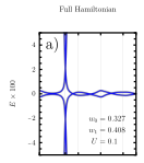
Refer to caption
(a)
Refer to caption
(b)
Refer to caption
(c)
Refer to caption
(d)
Refer to caption
(e)
Refer to caption
(f)
Refer to caption
(f)
Refer to caption
(g)
Refer to caption
(h)
Refer to caption
(i)
Refer to caption
(j)
Refer to caption
(k)
Refer to caption
(k)
Refer to caption
(l)
Refer to caption
(m)
Refer to caption
(n)
Refer to caption
(o)
Refer to caption
(p)
Figure 6: Various approximations used to compute the single-particle low-energy spectrum of TSTG in the presence of displacement field in the non-chiral limit. For each row, the first panel denotes the unapproximated spectrum (computed as in figs. 3a and 3c), while the second panel denotes the spectrum obtained numerically from the 8×88\times 8 Hamiltonian in eq. 178. In the third to fifth panels, we always approximate the spectrum away from the Dirac points of the MBZ using eq. 185. For the energy spectrum near the Dirac points, we employ the first, second, and third approximations of Appendix D.2.3 in the third, fourth, and fifth panels, respectively. We use a different cutoff Λ\Lambda for the each value of the displacement field UU, namely Λ=0.1\Lambda=0.1, 0.1750.175, and 0.20.2 for U=0.1U=0.1, 0.20.2, and 0.30.3, respectively. For each approximation, the bands are colored according to the overlap between the corresponding approximated and unapproximated single-particle wave functions. This overlap is always greater than 0.990.99. The values of the TSTG parameters are given as an inset for each plot.
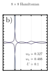
Refer to caption
(a)
Refer to caption
(b)
Refer to caption
(c)
Refer to caption
(d)
Refer to caption
(e)
Refer to caption
(f)
Refer to caption
(f)
Refer to caption
(g)
Refer to caption
(h)
Refer to caption
(i)
Refer to caption
(j)
Refer to caption
(k)
Refer to caption
(k)
Refer to caption
(l)
Refer to caption
(m)
Refer to caption
(n)
Refer to caption
(o)
Refer to caption
(p)
Figure 7: Various approximations used to compute the single-particle low-energy spectrum of TSTG in the presence of displacement field in the chiral limit. The meaning of the panels is the same as in fig. 6. All approximate models perform remarkably well, with no differences from the exact Hamiltonian visible by eye.
Having developed an intuition for the effect of the displacement field coupling on the TSTG single-particle spectrum, we now turn toward more quantitative perturbation schemes. As we are ultimately interested in the low-energy physics of TSTG, one approach would be to first consider the single-particle spectrum of the full TSTG Hamiltonian from eq. 87 and then project into its low-energy eigenstates. In our case, however, a better approach is to consider the TBG Hamiltonian of eq. 88 projected into its flat bands and then hybridize it with the high-velocity Dirac cone in the presence of displacement field.

D.2.1 Perturbative effect of the displacement field

We assume that w0≤0.8​w1w_{0}\leq 0.8w_{1}, which implies the existence of a sizable gap between the active bands (n=±1n=\pm 1) and the passive bands of the TBG Hamiltonian: in particular, the active band bandwidth ω\omega is much smaller that the gap Bernevig et al. 2020a. The approach of starting from the projected TBG single-particle Hamiltonian (henceforth denoted without a hat)

HTBG=∑|n|=1∑η,s∑𝐤∈MBZϵn,ηc^​(𝐤)​c^𝐤,n,η,s†​c^𝐤,n,η,s,H_{\mathrm{TBG}}=\sum_{\absolutevalue{n}=1}\sum_{\eta,s}\sum_{\mathbf{k}\in\mathrm{MBZ}}\epsilon_{n,\eta}^{\hat{c}}\left(\mathbf{k}\right)\hat{c}^{\dagger}_{\mathbf{k},n,\eta,s}\hat{c}_{\mathbf{k},n,\eta,s}, (172)

rather than the unprojected one is justified by using perturbation theory arguments. For the experimentally relevant values of the displacement field Hao et al. 2021 (corresponding to U<0.3U<0.3), we can develop a perturbation theory in UU for the hybridization between the two mirror-symmetry sectors. The hybridization between the TBG active bands and the Dirac cone Hamiltonian happens already at first order in UU, while mixing between the TBG active and passive bands happens only as a second order virtual process in UU.

The low-energy physics of TSTG is therefore governed by the Hamiltonian

H0=HTBG+H^D+H^U,H_{0}=H_{\mathrm{TBG}}+\hat{H}_{D}+\hat{H}_{U}, (173)

where the projected TBG Hamiltonian was given by eq. 172, while the Dirac cone and displacement field contributions are respectively given by

H^D=∑𝐤∈MBZη,s∑α,β∑i=13[hη​𝐪𝐢D,η​(𝐤)]α​β​b^𝐤,η​𝐪i,η,α,s†​b^𝐤,η​𝐪i,η,β,s,\hat{H}_{D}=\sum_{\begin{subarray}{c}\mathbf{k}\in\mathrm{MBZ}\\ \eta,s\end{subarray}}\sum_{\alpha,\beta}\sum_{i=1}^{3}\left[h^{D,\eta}_{\mathbf{\eta\mathbf{q}_{i}}}\left(\mathbf{k}\right)\right]_{\alpha\beta}\hat{b}^{\dagger}_{\mathbf{k},\eta\mathbf{q}_{i},\eta,\alpha,s}\hat{b}_{\mathbf{k},\eta\mathbf{q}_{i},\eta,\beta,s}, (174)

and

H^U=U2​∑𝐤∈MBZη,s∑α∑i=13∑|n|=1(uη​𝐪i​α;n​ηc^​(𝐤)​b^𝐤,η​𝐪i,η,α,s†​c^𝐤,n,η,s+uη​𝐪i​α;n​η∗c^​(𝐤)​c^𝐤,n,η,s†​b^𝐤,η​𝐪i,η,α,s).\hat{H}_{U}=\frac{U}{2}\sum_{\begin{subarray}{c}\mathbf{k}\in\mathrm{MBZ}\\ \eta,s\end{subarray}}\sum_{\alpha}\sum_{i=1}^{3}\sum_{\absolutevalue{n}=1}\left(u^{\hat{c}}_{\eta\mathbf{q}_{i}\alpha;n\eta}\left(\mathbf{k}\right)\hat{b}^{\dagger}_{\mathbf{k},\eta\mathbf{q}_{i},\eta,\alpha,s}\hat{c}_{\mathbf{k},n,\eta,s}+u^{*\hat{c}}_{\eta\mathbf{q}_{i}\alpha;n\eta}\left(\mathbf{k}\right)\hat{c}^{\dagger}_{\mathbf{k},n,\eta,s}\hat{b}_{\mathbf{k},\eta\mathbf{q}_{i},\eta,\alpha,s}\right). (175)

Among other things, we checked numerically the validity of the TSTG Hamiltonian from eq. 173 in the first two columns of figs. 6 and 7. The low-energy TSTG spectrum obtained from eq. 173 and the one obtained from H^0=H^TBG+H^D+H^U\hat{H}_{0}=\hat{H}_{\mathrm{TBG}}+\hat{H}_{D}+\hat{H}_{U} (i.e. starting from the unprojected TBG Hamiltonian) are consistent both in energy and eigenstates to an error smaller than 1%1\%. Moreover, as discussed in Appendix A.1, we have restricted to only three plane-wave states (i.e. 𝐐\mathbf{Q} points) in the expression of H^D\hat{H}_{D}. However, the eigenstates of the TBG active bands are evaluated in all generality on the 𝒬±\mathcal{Q}_{\pm} sublattice using the approximations discussed in Ref. Bernevig et al. 2020a.

For the sake of making this appendix self-contained, we briefly review the notation provided in section IV.3. The single-particle eigenstates of H0H_{0} for valley η\eta and spin ss labeled by mm are given by

|Ψη,s,m​(𝐤)⟩=[∑i=13∑α(ψi,αη,s,m​(𝐤)​b^𝐤,η​𝐪i,η,α,s†)+∑|n|=1ϕnη,s,m​(𝐤)​c^𝐤,n,η,s†]​|0⟩.\ket{\Psi^{\eta,s,m} \left( \vec{k} \right)}=\left[\sum_{i=1}^{3}\sum_{\alpha}\left(\psi^{\eta,s,m}_{i,\alpha}\left(\mathbf{k}\right)\hat{b}^{\dagger}_{\mathbf{k},\eta\mathbf{q}_{i},\eta,\alpha,s}\right)+\sum_{\absolutevalue{n}=1}\phi^{\eta,s,m}_{n}\left(\mathbf{k}\right)\hat{c}^{\dagger}_{\mathbf{k},n,\eta,s}\right]\ket{0}. (176)

In eq. 176, we have defined three two-component spinors on the sublattice space, ψiη,s,m​(𝐤)\psi^{\eta,s,m}_{i}\left(\mathbf{k}\right) (for i=1,2,3i=1,2,3), corresponding to the three Dirac points in the MBZ, and the two-component spinor in the space of the n=±1n=\pm 1 active TBG bands, ϕη,s,m​(𝐤)\phi^{\eta,s,m}\left(\mathbf{k}\right). We have also employed mm to label the different bands of H0H_{0}. The single-particle eigenvalue equation

H0​|Ψη,s,m​(𝐤)⟩=Eη,m​(𝐤)​|Ψη,s,m​(𝐤)⟩H_{0}\ket{\Psi^{\eta,s,m} \left( \vec{k} \right)}=E^{\eta,m}\left(\mathbf{k}\right)\ket{\Psi^{\eta,s,m} \left( \vec{k} \right)} (177)

can be written in matrix form as

(ℰη​(𝐤)U1†η​(𝐤)U2†η​(𝐤)U3†η​(𝐤)U1η​(𝐤)hη​𝐪𝟏D,η​(𝐤)𝟘𝟘U2η​(𝐤)𝟘hη​𝐪𝟐D,η​(𝐤)𝟘U3η​(𝐤)𝟘𝟘hη​𝐪𝟑D,η​(𝐤))​(ϕη,s,m​(𝐤)ψ1η,s,m​(𝐤)ψ2η,s,m​(𝐤)ψ3η,s,m​(𝐤))=Eη,m​(𝐤)​(ϕη,s,m​(𝐤)ψ1η,s,m​(𝐤)ψ2η,s,m​(𝐤)ψ3η,s,m​(𝐤))\begin{pmatrix}\mathcal{E}^{\eta}\left(\mathbf{k}\right)&U^{\dagger\eta}_{1}\left(\mathbf{k}\right)&U^{\dagger\eta}_{2}\left(\mathbf{k}\right)&U^{\dagger\eta}_{3}\left(\mathbf{k}\right)\\ U^{\eta}_{1}\left(\mathbf{k}\right)&h^{D,\eta}_{\mathbf{\eta\mathbf{q}_{1}}}\left(\mathbf{k}\right)&\mathbb{0}&\mathbb{0}\\ U^{\eta}_{2}\left(\mathbf{k}\right)&\mathbb{0}&h^{D,\eta}_{\mathbf{\eta\mathbf{q}_{2}}}\left(\mathbf{k}\right)&\mathbb{0}\\ U^{\eta}_{3}\left(\mathbf{k}\right)&\mathbb{0}&\mathbb{0}&h^{D,\eta}_{\mathbf{\eta\mathbf{q}_{3}}}\left(\mathbf{k}\right)\end{pmatrix}\begin{pmatrix}\phi^{\eta,s,m}\left(\mathbf{k}\right)\\ \psi^{\eta,s,m}_{1}\left(\mathbf{k}\right)\\ \psi^{\eta,s,m}_{2}\left(\mathbf{k}\right)\\ \psi^{\eta,s,m}_{3}\left(\mathbf{k}\right)\end{pmatrix}=E^{\eta,m}\left(\mathbf{k}\right)\begin{pmatrix}\phi^{\eta,s,m}\left(\mathbf{k}\right)\\ \psi^{\eta,s,m}_{1}\left(\mathbf{k}\right)\\ \psi^{\eta,s,m}_{2}\left(\mathbf{k}\right)\\ \psi^{\eta,s,m}_{3}\left(\mathbf{k}\right)\end{pmatrix} (178)

where we have defined the 2×22\times 2 diagonal energy matrix for the TBG active bands in valley η\eta

ℰη​(𝐤)=(ϵ+1,ηc^​(𝐤)00ϵ−1,ηc^​(𝐤))\mathcal{E}^{\eta}\left(\mathbf{k}\right)=\begin{pmatrix}\epsilon^{\hat{c}}_{+1,\eta}\left(\mathbf{k}\right)&0\\ 0&\epsilon^{\hat{c}}_{-1,\eta}\left(\mathbf{k}\right)\\ \end{pmatrix} (179)

as well as the displacement field 2×22\times 2 perturbation matrices

[Uiη​(𝐤)]α,n=U2​uη​𝐪i​α;n​ηc^​(𝐤),\left[U^{\eta}_{i}\left(\mathbf{k}\right)\right]_{\alpha,n}=\frac{U}{2}u^{\hat{c}}_{\eta\mathbf{q}_{i}\alpha;n\eta}\left(\mathbf{k}\right), (180)

for i=1,2,3i=1,2,3. In what follows, we will temporarily suppress the mm, η\eta, and ss indices as well as the momentum 𝐤\mathbf{k} parameter. In addition, we will introduce the following shorthand notation

hi≡hη​𝐪iD,η​(𝐤),h_{i}\equiv h_{\eta\mathbf{q}_{i}}^{D,\eta}\left(\mathbf{k}\right), (181)

for i=1,2,3i=1,2,3.

There are two regions of interest pertaining to the low-energy eigenstates of H0H_{0}. When 𝐤\mathbf{k} is away from the Dirac points, i.e. 𝐤∈𝒞η\mathbf{k}\in\mathcal{C}_{\eta}, where we have defined the region

𝒞η=MBZ∖⋃i=13Aηi\mathcal{C}_{\eta}=\mathrm{MBZ}\setminus\bigcup_{i=1}^{3}A_{\eta}^{i} (182)

in terms of the regions AηiA_{\eta}^{i} introduced in eq. 92, the hybridization between the eigenstates of H^D\hat{H}_{D} and the active bands of H^TBG\hat{H}_{\mathrm{TBG}} is suppressed by the difference in energy. One can therefore avoid solving the 8×88\times 8 Hamiltonian in eq. 178 and employ perturbation theory to find the effect of the displacement on the active bands in this region. When 𝐤\mathbf{k} is near any of the three Dirac point of H^D\hat{H}_{D} in the MBZ, i.e. 𝐤∈Aηi\mathbf{k}\in A_{\eta}^{i}, we can no longer ignore the effects of the Dirac cone bands and more refined approximation methods needs to be developed. We will now explore these two cases and attempt to solve the Hamiltonian in eq. 178.

D.2.2 Perturbation theory away from the Dirac points

When 𝐤∈𝒞η\mathbf{k}\in\mathcal{C}_{\eta}, the hybridization between the active TBG bands and the Dirac cone bands is suppressed by the difference in energy. We can therefore eliminate the ψi\psi_{i} spinors of eq. 178 by writing them in terms of the ϕ\phi spinors.

ψi=(E−hi)−1​Ui​ϕ.\psi_{i}=\left(E-h_{i}\right)^{-1}U_{i}\phi. (183)

This allows us to formulate our problem as a non-linear eigenvalue equation for ϕ\phi which simply reads

[ℰ+∑i=13Ui†​(E−hi)−1​Ui]​ϕ=E​ϕ.\left[\mathcal{E}+\sum_{i=1}^{3}U^{\dagger}_{i}\left(E-h_{i}\right)^{-1}U_{i}\right]\phi=E\phi. (184)

We expect the energy of the active bands to be only slightly changed by the hybridization with the Dirac cone Hamiltonian and have |E|≪|hi|=|𝐤−η​𝐪i|\absolutevalue{E}\ll\absolutevalue{h_i}=\absolutevalue{\vec{k} - \eta\vec{q}_i}. For the low-energy bands of H0H_{0} we can thus ignore the EE dependence in the denominator of the second term of eq. 184. This affords a major simplification as the Hamiltonians hih_{i} can be readily inverted. Introducing the notation 𝝈+=(σx,σy)\bm{\sigma}^{+}=\left(\sigma_{x},\sigma_{y}\right) and 𝝈−=(−σx,σy)\bm{\sigma}^{-}=\left(-\sigma_{x},\sigma_{y}\right) to denote the Pauli vector corresponding to the two valleys η=±\eta=\pm, the eigenvalue equation becomes

(ϵ+1,ηc^​(𝐤)+ℬ+1,+1η​(𝐤)ℬ+1,−1η​(𝐤)ℬ−1,+1η​(𝐤)ϵ−1,ηc^​(𝐤)+ℬ−1,−1η​(𝐤))​(ϕ+1η,s,m​(𝐤)ϕ−1η,s,m​(𝐤))=Eη,m​(𝐤)​(ϕ+1η,s,m​(𝐤)ϕ−1η,s,m​(𝐤)),\begin{pmatrix}\epsilon^{\hat{c}}_{+1,\eta}\left(\mathbf{k}\right)+\mathcal{B}_{+1,+1}^{\eta}\left(\mathbf{k}\right)&\mathcal{B}_{+1,-1}^{\eta}\left(\mathbf{k}\right)\\ \mathcal{B}_{-1,+1}^{\eta}\left(\mathbf{k}\right)&\epsilon^{\hat{c}}_{-1,\eta}\left(\mathbf{k}\right)+\mathcal{B}_{-1,-1}^{\eta}\left(\mathbf{k}\right)\\ \end{pmatrix}\begin{pmatrix}\phi^{\eta,s,m}_{+1}\left(\mathbf{k}\right)\\ \phi^{\eta,s,m}_{-1}\left(\mathbf{k}\right)\end{pmatrix}=E^{\eta,m}\left(\mathbf{k}\right)\begin{pmatrix}\phi^{\eta,s,m}_{+1}\left(\mathbf{k}\right)\\ \phi^{\eta,s,m}_{-1}\left(\mathbf{k}\right)\end{pmatrix}, (185)

where we have defined the displacement field perturbation matrix

ℬn​mη​(𝐤)=U24​∑i=13∑α,βuη​𝐪i​α;n​η∗c^​(𝐤)​[(𝐤−η​𝐪i)⋅𝝈η]α​β​uη​𝐪i​β;m​ηc^​(𝐤)|𝐤−η​𝐪i|2.\mathcal{B}^{\eta}_{nm}\left(\mathbf{k}\right)=\frac{U^{2}}{4}\sum_{i=1}^{3}\sum_{\alpha,\beta}\frac{u^{*\hat{c}}_{\eta\mathbf{q}_{i}\alpha;n\eta}\left(\mathbf{k}\right)\left[\left(\mathbf{k}-\eta\mathbf{q}_{i}\right)\cdot\bm{\sigma}^{\eta}\right]_{\alpha\beta}u^{\hat{c}}_{\eta\mathbf{q}_{i}\beta;m\eta}\left(\mathbf{k}\right)}{\absolutevalue{\vec{k} - \eta\vec{q}_i}^{2}}. (186)

As eq. 185 is only a 2×22\times 2 matrix, it can be readily diagonalized to obtain the low-energy band dispersion

Eη,±1=ϵ+1,ηc^+ϵ−1,ηc^+ℬ+1,+1η+ℬ−1,−1η±[ϵ+1,ηc^−ϵ−1,ηc^+ℬ+1,+1η−ℬ−1,−1η]2+ℬ−1,+1η​ℬ+1,−1η2.E^{\eta,\pm 1}=\frac{\epsilon^{\hat{c}}_{+1,\eta}+\epsilon^{\hat{c}}_{-1,\eta}+\mathcal{B}_{+1,+1}^{\eta}+\mathcal{B}_{-1,-1}^{\eta}\pm\sqrt{\left[\epsilon^{\hat{c}}_{+1,\eta}-\epsilon^{\hat{c}}_{-1,\eta}+\mathcal{B}_{+1,+1}^{\eta}-\mathcal{B}_{-1,-1}^{\eta}\right]^{2}+\mathcal{B}_{-1,+1}^{\eta}\mathcal{B}_{+1,-1}^{\eta}}}{2}. (187)
Refer to caption
(a)
Refer to caption
(b)
Refer to caption
(c)
Refer to caption
(d)
Refer to caption
(d)
Refer to caption
(e)
Refer to caption
(f)
Refer to caption
(g)
Figure 8: The amplitude of the mirror-symmetric operators in the lowest-energy single-particle eigenstates of TSTG. We consider the overlap between the unapproximated (|ψ⟩\ket{\psi}) and approximated (|ψapp⟩\ket{\psi_{\mathrm{app}}}) wave functions corresponding to the lowest-energy conduction band for valley η=+\eta=+ in the MBZ of TSTG. The approximated wave function |ψapp⟩\ket{\psi_{\mathrm{app}}} is obtained directly from |ψ⟩\ket{\psi} by setting the amplitudes of all mirror-antisymmetric creation operators to zero (i.e. |ψapp⟩=1+mz2​|ψ⟩\ket{\psi_{\mathrm{app}}}=\frac{1+m_{z}}{2}\ket{\psi}). The boundaries of the A+iA_{+}^{i} zones (for i=1,2,3i=1,2,3) are shown with red dashed lines. We consider the nonchiral limit (w0/w1=0.8w_{0}/w_{1}=0.8, w1=0.408w_{1}=0.408) in panels a)-c) and the chiral limit (w0=0w_{0}=0, w1=0.408w_{1}=0.408) in panels d)-f). The values of the displacement field are U=0.1U=0.1 in panels a) and d), U=0.2U=0.2 in panels b) and e), and U=0.3U=0.3 panels in c) and f). Away from the high-velocity Dirac points in the TSTG MBZ, the weight of the mirror-antisymmetric operators in the low-energy eigenstates is negligible.

The corresponding eigenstates can be found from the ϕ\phi spinors and eq. 183. We prove the validity of the approximation from eq. 185 numerically in the third, fourth and fifth columns of figs. 6 and 7 in both the non-chiral and (first) chiral limits, respectively. However, a further approximation can be used: as shown in fig. 8, the weight of the mirror-antisymmetric operators is small enough in this region of the MBZ to approximate ψi≈0\psi_{i}\approx 0. The effects of the displacement field for 𝐤∈𝒞η\mathbf{k}\in\mathcal{C}_{\eta} can then be captured by the following effective Hamiltonian which is second order in the displacement field

HU(c^)=∑|n|,|m|=1η,s∑𝐤∈𝒞ηℬn​mη​(𝐤)​c^𝐤,n,η,s†​c^𝐤,n′,η,s.H^{\left(\hat{c}\right)}_{U}=\sum_{\begin{subarray}{c}\absolutevalue{n},\absolutevalue{m}=1\\ \eta,s\end{subarray}}\sum_{\begin{subarray}{c}\mathbf{k}\in\mathcal{C}_{\eta}\end{subarray}}\mathcal{B}^{\eta}_{nm}\left(\mathbf{k}\right)\hat{c}^{\dagger}_{\mathbf{k},n,\eta,s}\hat{c}_{\mathbf{k},n^{\prime},\eta,s}. (188)

Finally, we note that if U2/|𝐤−η​𝐪i|≪ωU^{2}/\absolutevalue{\vec{k} - \eta\vec{q}_i}\ll\omega for i=1,2,3i=1,2,3, then the active TBG band states will not be significantly perturbed by the displacement field.

D.2.3 Perturbation theory near the Dirac points

Near any of the three Dirac points in the MBZ, the hybridization between the TBG active bands and the folded Dirac cone Hamiltonian is significant. If 𝐤\mathbf{k} is near the jj-th Dirac point in the MBZ (i.e. 𝐤∈Aηj\mathbf{k}\in A_{\eta}^{j}), we will have |hj|≪1\absolutevalue{h_j}\ll 1, but |hi|≈3\absolutevalue{h_i}\approx\sqrt{3}, for i≠ji\neq j. This implies that while the hybridization between the TBG active bands and the jj-th Dirac Hamiltonian will be relevant, there will be little to no mixing with the Dirac cone bands stemming from the other two Dirac points of H^D\hat{H}_{D} in the MBZ. We can therefore approximate ψi≈0\psi_{i}\approx 0 for i≠ji\neq j and write the single-particle TSTG wave functions as

|Ψη,s,m​(𝐤)⟩=[∑α(ψj,αη,s,m​(𝐤)​b^𝐤,η​𝐪j,η,α,s†)+∑n=±1ϕnη,s,m​(𝐤)​c^𝐤,n,η,s†]​|0⟩.\ket{\Psi^{\eta,s,m} \left( \vec{k} \right)}=\left[\sum_{\alpha}\left(\psi^{\eta,s,m}_{j,\alpha}\left(\mathbf{k}\right)\hat{b}^{\dagger}_{\mathbf{k},\eta\mathbf{q}_{j},\eta,\alpha,s}\right)+\sum_{n=\pm 1}\phi^{\eta,s,m}_{n}\left(\mathbf{k}\right)\hat{c}^{\dagger}_{\mathbf{k},n,\eta,s}\right]\ket{0}. (189)

reflecting the four bands per spin per valley which are relevant for the low-energy of TSTG, namely the two TBG active bands and two Dirac cone bands. The eigenvalue equation H0​|Ψη,s,m​(𝐤)⟩=Eη,m​(𝐤)​|Ψη,s,m​(𝐤)⟩H_{0}\ket{\Psi^{\eta,s,m} \left( \vec{k} \right)}=E^{\eta,m}\left(\mathbf{k}\right)\ket{\Psi^{\eta,s,m} \left( \vec{k} \right)} can then be written as a 4×44\times 4 matrix eigenvalue equation

(ℰη​(𝐤)Uj†η​(𝐤)Ujη​(𝐤)hη​𝐪jD,η​(𝐤))​(ϕη,s,m​(𝐤)ψjη,s,m​(𝐤))=Eη,m​(𝐤)​(ϕη,s,m​(𝐤)ψjη,s,m​(𝐤)).\begin{pmatrix}\mathcal{E}^{\eta}\left(\mathbf{k}\right)&U^{\dagger\eta}_{j}\left(\mathbf{k}\right)\\ U^{\eta}_{j}\left(\mathbf{k}\right)&h^{D,\eta}_{\eta\mathbf{q}_{j}}\left(\mathbf{k}\right)\\ \end{pmatrix}\begin{pmatrix}\phi^{\eta,s,m}\left(\mathbf{k}\right)\\ \psi^{\eta,s,m}_{j}\left(\mathbf{k}\right)\end{pmatrix}=E^{\eta,m}\left(\mathbf{k}\right)\begin{pmatrix}\phi^{\eta,s,m}\left(\mathbf{k}\right)\\ \psi^{\eta,s,m}_{j}\left(\mathbf{k}\right)\end{pmatrix}. (190)

We will call this the first approximation. While this Hamiltonian cannot be solved analytically, we can employ a series of approximations to make the computations tractable. We begin by eliminating the ϕ\phi spinor to obtain a nonlinear eigenvalue equation for ψj\psi_{j}

[hj+Uj​E−ϵ+c^+ϵ−c^2+ϵ+c^−ϵ−c^2​σz(E−ϵ+c^+ϵ−c^2)2−(ϵ+c^−ϵ−c^2)2​Uj†]​ψj=E​ψj,\left[h_{j}+U_{j}\frac{E-\frac{\epsilon^{\hat{c}}_{+}+\epsilon^{\hat{c}}_{-}}{2}+\frac{\epsilon^{\hat{c}}_{+}-\epsilon^{\hat{c}}_{-}}{2}\sigma_{z}}{\left(E-\frac{\epsilon^{\hat{c}}_{+}+\epsilon^{\hat{c}}_{-}}{2}\right)^{2}-\left(\frac{\epsilon^{\hat{c}}_{+}-\epsilon^{\hat{c}}_{-}}{2}\right)^{2}}U^{\dagger}_{j}\right]\psi_{j}=E\psi_{j}, (191)

where we have suppressed the valley index and made the dependence on the 𝐤\mathbf{k} parameter implicit. We then ignore the term ϵ+c^+ϵ−c^2\frac{\epsilon^{\hat{c}}_{+}+\epsilon^{\hat{c}}_{-}}{2} to first order in EE (an approximation which is exact in the chiral limit, where ϵ−c^=−ϵ+c^\epsilon^{\hat{c}}_{-}=-\epsilon^{\hat{c}}_{+}), obtaining

[hj+Uj​E+ϵ+c^−ϵ−c^2​σzE2−(ϵ+c^−ϵ−c^2)2​Uj†]​ψj=E​ψj.\left[h_{j}+U_{j}\frac{E+\frac{\epsilon^{\hat{c}}_{+}-\epsilon^{\hat{c}}_{-}}{2}\sigma_{z}}{E^{2}-\left(\frac{\epsilon^{\hat{c}}_{+}-\epsilon^{\hat{c}}_{-}}{2}\right)^{2}}U^{\dagger}_{j}\right]\psi_{j}=E\psi_{j}. (192)

The solution to eq. 192 can be found as an asymptotic series in the small parameter ϵ+c^−ϵ−c^2\frac{\epsilon^{\hat{c}}_{+}-\epsilon^{\hat{c}}_{-}}{2}: to first order in ϵ+c^−ϵ−c^2\frac{\epsilon^{\hat{c}}_{+}-\epsilon^{\hat{c}}_{-}}{2}, the nonlinear eigenvalue equation becomes

[hj+Uj​E+ϵ+c^−ϵ−c^2​σzE2​Uj†]​ψj=E​ψj,\left[h_{j}+U_{j}\frac{E+\frac{\epsilon^{\hat{c}}_{+}-\epsilon^{\hat{c}}_{-}}{2}\sigma_{z}}{E^{2}}U^{\dagger}_{j}\right]\psi_{j}=E\psi_{j}, (193)

an approximation which we call the second approximation. Solving this equation is still impossible to do analytically, so we take one further simplification and ignore the ϵ+c^−ϵ−c^2\frac{\epsilon^{\hat{c}}_{+}-\epsilon^{\hat{c}}_{-}}{2} term altogether to afford the third approximation

[hj+Uj​Uj†E]​ψj=E​ψj.\left[h_{j}+\frac{U_{j}U^{\dagger}_{j}}{E}\right]\psi_{j}=E\psi_{j}. (194)

Since hjh_{j} is a 2×22\times 2 matrix, finding the energies of this equation essentially amounts to solving for the roots of a fourth-order polynomial, a cumbersome task to do analytically. In the chiral limit however, under the gauge-fixing of eq. 139, we have that

∑β(σz)α​β​[Uj]β,n=η​∑n′[Uj]α,n′​(σy)n′​n,\sum_{\beta}\left(\sigma_{z}\right)_{\alpha\beta}\left[U_{j}\right]_{\beta,n}=\eta\sum_{n^{\prime}}\left[U_{j}\right]_{\alpha,n^{\prime}}\left(\sigma_{y}\right)_{n^{\prime}n}, (195)

which translates to σz​Uj​Uj†​σz=Uj​Uj†\sigma_{z}U_{j}U_{j}^{\dagger}\sigma_{z}=U_{j}U_{j}^{\dagger}, implying that the term Uj​Uj†U_{j}U_{j}^{\dagger} is essentially a 2×22\times 2 diagonal matrix

Uj​Uj†=(A00D),U_{j}U^{\dagger}_{j}=\begin{pmatrix}A&0\\ 0&D\end{pmatrix}, (196)

where AA and DD are real functions of 𝐤\mathbf{k}, obtained from the moiré eigenstates. The characteristic equation of the third approximation

det⁡[E2−E​hj−(A00D)]=0\det\left[E^{2}-Eh_{j}-\begin{pmatrix}A&0\\ 0&D\end{pmatrix}\right]=0 (197)

is equivalent to finding the roots of a second order polynomial in E2E^{2}, an equation which can be readily solved analytically.

We note that the validity of eq. 190 (i.e. the first approximation), as well as of the second and third approximations was checked numerically in figs. 6 and 7 in the third, fourth and fifth columns, respectively. In what follows, we will restrict to the first approximation from eq. 190 and write the corresponding projected displacement field Hamiltonian as

HU(b^​c^)=U2∑i=13∑𝐤∈Aηi∑|n|=1α(uη​𝐪i​α;n​ηc^(𝐤)b^𝐤,η​𝐪i,η,α,s†c^𝐤,n,η,s+h.c.).H^{\left(\hat{b}\hat{c}\right)}_{U}=\frac{U}{2}\sum_{i=1}^{3}\sum_{\mathbf{k}\in A^{i}_{\eta}}\sum_{\begin{subarray}{c}\absolutevalue{n}=1\\ \alpha\end{subarray}}\left(u^{\hat{c}}_{\eta\mathbf{q}_{i}\alpha;n\eta}\left(\mathbf{k}\right)\hat{b}^{\dagger}_{\mathbf{k},\eta\mathbf{q}_{i},\eta,\alpha,s}\hat{c}_{\mathbf{k},n,\eta,s}+\mathrm{h.c.}\right). (198)

In terms of the energy band basis, the projected displacement field Hamiltonian reads

HU(b^​c^)=∑|n|,|m|=1η,s∑|δ​𝐤|≤Λ[Nm​nη(δ𝐤)b^δ​𝐤+η​𝐪1,m,η,s†c^δ​𝐤+η​𝐪1,n,η,s+h.c.],H^{\left(\hat{b}\hat{c}\right)}_{U}=\sum_{\begin{subarray}{c}\absolutevalue{n},\absolutevalue{m}=1\\ \eta,s\end{subarray}}\sum_{\absolutevalue{\delta\vec{k}}\leq\Lambda}\left[N^{\eta}_{mn}\left(\delta\mathbf{k}\right)\hat{b}^{\dagger}_{\delta\mathbf{k}+\eta\mathbf{q}_{1},m,\eta,s}\hat{c}_{\delta\mathbf{k}+\eta\mathbf{q}_{1},n,\eta,s}+\mathrm{h.c.}\right], (199)

where we have defined the displacement field overlap matrix

Nm​nη​(δ​𝐤)=∑αuη​𝐪1​α;m​η∗b^​(δ​𝐤+η​𝐪1)​uη​𝐪1​α;n​ηc^​(δ​𝐤+η​𝐪1).N^{\eta}_{mn}\left(\delta\mathbf{k}\right)=\sum_{\alpha}u^{*\hat{b}}_{\eta\mathbf{q}_{1}\alpha;m\eta}\left(\delta\mathbf{k}+\eta\mathbf{q}_{1}\right)u^{\hat{c}}_{\eta\mathbf{q}_{1}\alpha;n\eta}\left(\delta\mathbf{k}+\eta\mathbf{q}_{1}\right). (200)

For simplicity, in eq. 199 we have used the periodicity of the energy band fermion operators eq. 97, as well as the embedding relation of the single-particle wave functions eq. 96 to bring together the zones AηiA_{\eta}^{i} (for i=1,2,3i=1,2,3) into a full circular region around the η​𝐪1\eta\mathbf{q}_{1} point.

Appendix E Gauge-fixing the single-particle projected Hamiltonian

The discrete symmetries of the single-particle Hamiltonian from Appendix B together with the gauge-fixing conditions in Appendix C directly determine the explicit forms of the various terms of the single-particle projected TSTG Hamiltonian. The goal of this appendix is to parameterize the various terms appearing in the single-particle projected TSTG Hamiltonian from eq. 32 of section IV.4. The resulting parameterizations will be used for the unambiguous identification of the continuous symmetry groups of the projected many-body TSTG Hamiltonian in Appendix G, together with their corresponding generators.

In what follows, we will find it useful to employ a series of conventions pertaining to the energy band operators c^𝐤,n,η,s†\hat{c}^{\dagger}_{\mathbf{k},n,\eta,s} and b^𝐤,n,η,s†\hat{b}^{\dagger}_{\mathbf{k},n,\eta,s}. For both mirror-symmetry sector operators, we will use ζa\zeta^{a} (with a=0,x,y,za=0,x,y,z) to denote the identity and Pauli matrices in the energy band subspace (restricting to the pair of bands n=±1n=\pm 1), τa\tau^{a} (with a=0,x,y,za=0,x,y,z) for the valley subspace, and sas^{a} (with a=0,x,y,za=0,x,y,z) for the spin subspace.

E.1 Parameterized forms of the single-particle projected TBG and Dirac Hamiltonian

Independent of the gauge chosen in Appendix C, the form of the Hamiltonians HTBGH_{\mathrm{TBG}} and HDH_{D} in the energy band basis is constrained by the symmetries discussed in Appendix B. For the sake of completeness, we will list the resulting parameterizations here.

E.1.1 Parameterization of HTBGH_{\mathrm{TBG}}

The energies of the TBG active bands ϵn,ηc^​(𝐤)\epsilon_{n,\eta}^{\hat{c}}\left(\mathbf{k}\right) can be viewed as the elements of a 𝐤\mathbf{k}-dependent matrix which we dub the TBG energy band matrix and which is diagonal in the valley and energy band subspaces. The (unprojected) TBG Hamiltonian from eq. 88 is symmetric under the combined C2​z​PC_{2z}P transformation

{H^TBG,C2​z​P}=0.\left\{\hat{H}_{\mathrm{TBG}},C_{2z}P\right\}=0. (201)

This implies that ϵn,ηc^​(𝐤)=−ϵ−n,−ηc^​(𝐤)\epsilon_{n,\eta}^{\hat{c}}\left(\mathbf{k}\right)=-\epsilon_{-n,-\eta}^{\hat{c}}\left(\mathbf{k}\right) and so the TBG energy band matrix can be parameterized as

ϵn,ηc^​(𝐤)=[ζz​τ0]n​n,η​η​β0c^​(𝐤)+[ζ0​τz]n​n,η​η​β1c^​(𝐤),\epsilon_{n,\eta}^{\hat{c}}\left(\mathbf{k}\right)=\left[\zeta^{z}\tau^{0}\right]_{nn,\eta\eta}\beta^{\hat{c}}_{0}\left(\mathbf{k}\right)+\left[\zeta^{0}\tau^{z}\right]_{nn,\eta\eta}\beta^{\hat{c}}_{1}\left(\mathbf{k}\right), (202)

or in matrix notation

ϵc^​(𝐤)=ζz​τ0​β0c^​(𝐤)+ζ0​τz​β1c^​(𝐤).\epsilon^{\hat{c}}\left(\mathbf{k}\right)=\zeta^{z}\tau^{0}\beta^{\hat{c}}_{0}\left(\mathbf{k}\right)+\zeta^{0}\tau^{z}\beta^{\hat{c}}_{1}\left(\mathbf{k}\right). (203)

The functions β0,1c^​(𝐤)\beta^{\hat{c}}_{0,1}\left(\mathbf{k}\right) in eq. 203 represent real function whose exact form depends on the TBG band energies

β0c^​(𝐤)=ϵ+1,+c^​(𝐤)+ϵ+1,−c^​(𝐤)−ϵ−1,+c^​(𝐤)−ϵ−1,−c^​(𝐤)4β1c^​(𝐤)=ϵ+1,+c^​(𝐤)−ϵ+1,−c^​(𝐤)+ϵ−1,+c^​(𝐤)−ϵ−1,−c^​(𝐤)4\begin{split}\beta^{\hat{c}}_{0}\left(\mathbf{k}\right)&=\frac{\epsilon_{+1,+}^{\hat{c}}\left(\mathbf{k}\right)+\epsilon_{+1,-}^{\hat{c}}\left(\mathbf{k}\right)-\epsilon_{-1,+}^{\hat{c}}\left(\mathbf{k}\right)-\epsilon_{-1,-}^{\hat{c}}\left(\mathbf{k}\right)}{4}\\ \beta^{\hat{c}}_{1}\left(\mathbf{k}\right)&=\frac{\epsilon_{+1,+}^{\hat{c}}\left(\mathbf{k}\right)-\epsilon_{+1,-}^{\hat{c}}\left(\mathbf{k}\right)+\epsilon_{-1,+}^{\hat{c}}\left(\mathbf{k}\right)-\epsilon_{-1,-}^{\hat{c}}\left(\mathbf{k}\right)}{4}\end{split} (204)

Additionally, as a consequence of the C2​zC_{2z} commuting symmetry of H^TBG\hat{H}_{\mathrm{TBG}}, the TBG energy bands obey ϵn,ηc^​(𝐤)=−ϵn,−ηc^​(−𝐤)\epsilon_{n,\eta}^{\hat{c}}\left(\mathbf{k}\right)=-\epsilon_{n,-\eta}^{\hat{c}}\left(-\mathbf{k}\right), which further imposes that

β0c^​(𝐤)=β0c^​(−𝐤)andβ1c^​(𝐤)=−β1c^​(−𝐤).\beta^{\hat{c}}_{0}\left(\mathbf{k}\right)=\beta^{\hat{c}}_{0}\left(-\mathbf{k}\right)\qquad\text{and}\qquad\beta^{\hat{c}}_{1}\left(\mathbf{k}\right)=-\beta^{\hat{c}}_{1}\left(-\mathbf{k}\right). (205)

In the (first) chiral limit (w0=0w_{0}=0), the projected TBG Hamiltonian is also symmetric under the chiral transformation

{HTBG,C}=0.\left\{H_{\mathrm{TBG}},C\right\}=0. (206)

In this case, the band energies additionally satisfy ϵn,ηc^​(𝐤)=ϵ−n,ηc^​(𝐤)\epsilon_{n,\eta}^{\hat{c}}\left(\mathbf{k}\right)=\epsilon_{-n,\eta}^{\hat{c}}\left(\mathbf{k}\right), and thus β1c^​(𝐤)=0\beta^{\hat{c}}_{1}\left(\mathbf{k}\right)=0. In the chiral limit, the TBG energy band matrix can be written in the simple form

ϵc^​(𝐤)=ζz​τ0​β0c^​(𝐤).\epsilon^{\hat{c}}\left(\mathbf{k}\right)=\zeta^{z}\tau^{0}\beta^{\hat{c}}_{0}\left(\mathbf{k}\right). (207)

E.1.2 Parameterization of HDH_{D}

Similar to the active bands of HTBGH_{\mathrm{TBG}}, we can also view the band energies of the projected Dirac Hamiltonian from section IV.4 as the elements of a matrix diagonal in the energy band and valley subspaces. The exact form of the Dirac energy bands from eq. 35 allows the following straight-forward parameterization

ϵn,ηb^​(δ​𝐤)=[ζz​τ0]n​n,η​η​|δ​𝐤|.\epsilon_{n,\eta}^{\hat{b}}\left(\delta\mathbf{k}\right)=\left[\zeta^{z}\tau^{0}\right]_{nn,\eta\eta}\absolutevalue{\delta\vec{k}}. (208)

E.2 Parameterization of the projected displacement field Hamiltonian

As shown in Appendix D, the projected displacement field Hamiltonian has two contributions, HU(b^​c^)H_{U}^{\left(\hat{b}\hat{c}\right)} and HU(c^)H_{U}^{\left(\hat{c}\right)}, which are defined in disjoint regions of the MBZ, one close and one away from the Dirac points, and which are linear and quadratic in the displacement field parameter UU, respectively. We will now discuss the parameterized forms for each contribution.

E.2.1 Parameterized form of HU(b^​c^)H_{U}^{\left(\hat{b}\hat{c}\right)}

The first contribution to the displacement field Hamiltonian from eq. 199 is written in terms of the energy band basis operators of the TBG and Dirac cone sectors and the displacement field overlap matrix N⁡(δ​𝐤)N\left(\delta\mathbf{k}\right), whose exact form was given in eq. 200. Without explicitly solving for N⁡(δ​𝐤)N\left(\delta\mathbf{k}\right), we will now analyze the constraints imposed on its form by the symmetries of TSTG presented in Appendix B in conjunction with the 𝐤\mathbf{k}-independent sewing matrices fixed in Appendix C.

  1. 1.

    The antiunitary C2​z​TC_{2z}T symmetry of TSTG has the same 𝐤\mathbf{k}-independent sewing matrix for both the TBG and Dirac cone eigenstates, i.e. Bb^C2​z​T=Bc^C2​z​T=ζ0​τ0B_{\hat{b}}^{C_{2z}T}=B_{\hat{c}}^{C_{2z}T}=\zeta^{0}\tau^{0}. Using the shorthand notation from eq. 137, we obtain

    Nm​nη​(δ​𝐤)=U2​∑αuη​𝐪1​α;m​η∗b^​(δ​𝐤+η​𝐪1)​uη​𝐪1​α;n​ηc^​(δ​𝐤+η​𝐪1)\displaystyle N^{\eta}_{mn}\left(\delta\mathbf{k}\right)=\frac{U}{2}\sum_{\alpha}u^{*\hat{b}}_{\eta\mathbf{q}_{1}\alpha;m\eta}\left(\delta\mathbf{k}+\eta\mathbf{q}_{1}\right)u^{\hat{c}}_{\eta\mathbf{q}_{1}\alpha;n\eta}\left(\delta\mathbf{k}+\eta\mathbf{q}_{1}\right)
    =\displaystyle= U2​∑α,η1,η2[um​η1†b^​(δ​𝐤+η1​𝐪1)​[D†​(C2​z​T)]η​η1]η​𝐪1​α​[[D⁡(C2​z​T)]η​η2​un​η2c^​(δ​𝐤+η2​𝐪1)]η​𝐪1​α\displaystyle\frac{U}{2}\sum_{\alpha,\eta_{1},\eta_{2}}\left[u^{\dagger\hat{b}}_{m\eta_{1}}\left(\delta\mathbf{k}+\eta_{1}\mathbf{q}_{1}\right)\left[D^{\dagger}\left(C_{2z}T\right)\right]_{\eta\eta_{1}}\right]_{\eta\mathbf{q}_{1}\alpha}\left[\left[D\left(C_{2z}T\right)\right]_{\eta\eta_{2}}u^{\hat{c}}_{n\eta_{2}}\left(\delta\mathbf{k}+\eta_{2}\mathbf{q}_{1}\right)\right]_{\eta\mathbf{q}_{1}\alpha}
    =\displaystyle= U2​∑α,η1,η2m′,n′[Bb^†C2​z​T]m​η,m′​η1​uη1​𝐪1​α;m′​η1b^​(δ​𝐤+η1​𝐪1)​uη2​𝐪1​α;n′​η2∗c^​(δ​𝐤+η2​𝐪1)​[Bc^C2​z​T]n′​η2,n​η,\displaystyle\frac{U}{2}\sum_{\begin{subarray}{c}\alpha,\eta_{1},\eta_{2}\\ m^{\prime},n^{\prime}\end{subarray}}\left[B_{\hat{b}}^{\dagger C_{2z}T}\right]_{m\eta,m^{\prime}\eta_{1}}u^{\hat{b}}_{\eta_{1}\mathbf{q}_{1}\alpha;m^{\prime}\eta_{1}}\left(\delta\mathbf{k}+\eta_{1}\mathbf{q}_{1}\right)u^{*\hat{c}}_{\eta_{2}\mathbf{q}_{1}\alpha;n^{\prime}\eta_{2}}\left(\delta\mathbf{k}+\eta_{2}\mathbf{q}_{1}\right)\left[B_{\hat{c}}^{C_{2z}T}\right]_{n^{\prime}\eta_{2},n\eta}, (209)

    Equivalently, eq. 209 can be written in matrix form as

    N⁡(δ​𝐤)=(ζ0​τ0)​N∗​(δ​𝐤)​(ζ0​τ0)=N∗​(δ​𝐤).N\left(\delta\mathbf{k}\right)=\left(\zeta^{0}\tau^{0}\right)N^{*}\left(\delta\mathbf{k}\right)\left(\zeta^{0}\tau^{0}\right)=N^{*}\left(\delta\mathbf{k}\right). (210)

    proving that the displacement field overlap matrix is real.

  2. 2.

    In the (first) chiral limit, both the TBG and the Dirac cone Hamiltonians are symmetric under the chiral transformation CC, which has the 𝐤\mathbf{k}-independent sewing matrices Bb^C=Bc^C=ζy​τzB_{\hat{b}}^{C}=B_{\hat{c}}^{C}=\zeta^{y}\tau^{z}. Correspondingly, the displacement field overlap matrix obeys

    Nm​nη(δ𝐤)=U2∑αuη​𝐪1​α;m​ηb^∗(δ𝐤+η𝐪1)uη​𝐪1​α;n​ηc^(δ𝐤+η𝐪1)\displaystyle N^{\eta}_{mn}\left(\delta\mathbf{k}\right)=\frac{U}{2}\sum_{\alpha}u^{\hat{b}*}_{\eta\mathbf{q}_{1}\alpha;m\eta}\left(\delta\mathbf{k}+\eta\mathbf{q}_{1}\right)u^{\hat{c}}_{\eta\mathbf{q}_{1}\alpha;n\eta}\left(\delta\mathbf{k}+\eta\mathbf{q}_{1}\right)
    =\displaystyle= U2​∑α,η1,η2[um​η1†b^​(δ​𝐤+η1​𝐪1)​[D†​(C)]η​η1]η​𝐪1​α​[[D⁡(C)]η​η2​un​η2c^​(δ​𝐤+η2​𝐪1)]η​𝐪1​α\displaystyle\frac{U}{2}\sum_{\alpha,\eta_{1},\eta_{2}}\left[u^{\dagger\hat{b}}_{m\eta_{1}}\left(\delta\mathbf{k}+\eta_{1}\mathbf{q}_{1}\right)\left[D^{\dagger}\left(C\right)\right]_{\eta\eta_{1}}\right]_{\eta\mathbf{q}_{1}\alpha}\left[\left[D\left(C\right)\right]_{\eta\eta_{2}}u^{\hat{c}}_{n\eta_{2}}\left(\delta\mathbf{k}+\eta_{2}\mathbf{q}_{1}\right)\right]_{\eta\mathbf{q}_{1}\alpha}
    =\displaystyle= U2​∑α,η1,η2m′,n′[Bb^†C]m​η,m′​η1​uη1​𝐪1​α;m′​η1∗b^​(δ​𝐤+η1​𝐪1)​uη2​𝐪1​α;n′​η2c^​(δ​𝐤+η2​𝐪1)​[Bc^C]n′​η2,n​η,\displaystyle\frac{U}{2}\sum_{\begin{subarray}{c}\alpha,\eta_{1},\eta_{2}\\ m^{\prime},n^{\prime}\end{subarray}}\left[B_{\hat{b}}^{\dagger C}\right]_{m\eta,m^{\prime}\eta_{1}}u^{*\hat{b}}_{\eta_{1}\mathbf{q}_{1}\alpha;m^{\prime}\eta_{1}}\left(\delta\mathbf{k}+\eta_{1}\mathbf{q}_{1}\right)u^{\hat{c}}_{\eta_{2}\mathbf{q}_{1}\alpha;n^{\prime}\eta_{2}}\left(\delta\mathbf{k}+\eta_{2}\mathbf{q}_{1}\right)\left[B_{\hat{c}}^{C}\right]_{n^{\prime}\eta_{2},n\eta}, (211)

    which in matrix form is equivalent to

    N⁡(δ​𝐤)=(ζy​τz)​N​(δ​𝐤)​(ζy​τz).N\left(\delta\mathbf{k}\right)=\left(\zeta^{y}\tau^{z}\right)N\left(\delta\mathbf{k}\right)\left(\zeta^{y}\tau^{z}\right). (212)

The displacement field overlap matrix is diagonal in valley subspace and, as a consequence of eq. 210, its elements are real. It can therefore always be parameterized as

N⁡(δ​𝐤)=∑b∈{0,z}ζ0​τb​λ0​b(b^​c^)​(δ​𝐤)+ζx​τb​λx​b(b^​c^)​(δ​𝐤)+i​ζy​τb​λy​b(b^​c^)​(δ​𝐤)+ζz​τb​λz​b(b^​c^)​(δ​𝐤),N\left(\delta\mathbf{k}\right)=\sum_{b\in\left\{0,z\right\}}\zeta^{0}\tau^{b}\lambda^{\left(\hat{b}\hat{c}\right)}_{0b}\left(\delta\mathbf{k}\right)+\zeta^{x}\tau^{b}\lambda^{\left(\hat{b}\hat{c}\right)}_{xb}\left(\delta\mathbf{k}\right)+i\zeta^{y}\tau^{b}\lambda^{\left(\hat{b}\hat{c}\right)}_{yb}\left(\delta\mathbf{k}\right)+\zeta^{z}\tau^{b}\lambda^{\left(\hat{b}\hat{c}\right)}_{zb}\left(\delta\mathbf{k}\right), (213)

where λa​b(b^​c^)​(δ​𝐤)\lambda^{\left(\hat{b}\hat{c}\right)}_{ab}\left(\delta\mathbf{k}\right) (for a=0,x,y,za=0,x,y,z and b=0,zb=0,z) represent generic real functions, whose exact form depends on the single-particle wave functions of the TBG and Dirac Hamiltonians. Additionally, in the (first) chiral limit, due to the constraint imposed by eq. 212, λa​b(b^​c^)​(δ​𝐤)=0\lambda^{\left(\hat{b}\hat{c}\right)}_{ab}\left(\delta\mathbf{k}\right)=0 for a=x,za=x,z and b=0,zb=0,z and so the displacement field overlap matrix must be given by

N⁡(δ​𝐤)=ζ0​τ0​λ00(b^​c^)​(δ​𝐤)+i​ζy​τ0​λy​0(b^​c^)​(δ​𝐤)+ζ0​τz​λ0​z(b^​c^)​(δ​𝐤)+i​ζy​τz​λy​z(b^​c^)​(δ​𝐤).N\left(\delta\mathbf{k}\right)=\zeta^{0}\tau^{0}\lambda^{\left(\hat{b}\hat{c}\right)}_{00}\left(\delta\mathbf{k}\right)+i\zeta^{y}\tau^{0}\lambda^{\left(\hat{b}\hat{c}\right)}_{y0}\left(\delta\mathbf{k}\right)+\zeta^{0}\tau^{z}\lambda^{\left(\hat{b}\hat{c}\right)}_{0z}\left(\delta\mathbf{k}\right)+i\zeta^{y}\tau^{z}\lambda^{\left(\hat{b}\hat{c}\right)}_{yz}\left(\delta\mathbf{k}\right). (214)

E.2.2 Parameterized form of HU(c^)H_{U}^{\left(\hat{c}\right)}

The matrix ℬ⁡(𝐤)\mathcal{B}\left(\mathbf{k}\right) given in eq. 186 governs the second-order contribution to the displacement field projected Hamiltonian, away from the Dirac points. Here, we derive its parameterized form in a similar fashion to N⁡(δ​𝐤)N\left(\delta\mathbf{k}\right).

  1. 1.

    Owing to the antiunitary C2​z​TC_{2z}T symmetry of the TBG Hamiltonian with the 𝐤\mathbf{k}-independent sewing matrix Bc^C2​z​T=ζ0​τ0B_{\hat{c}}^{C_{2z}T}=\zeta^{0}\tau^{0}, the matrix ℬ⁡(𝐤)\mathcal{B}\left(\mathbf{k}\right) obeys

    ℬn​mη​(𝐤)=U24​∑i=13∑α,βuη​𝐪i​α;n​η∗c^​(𝐤)​[(𝐤−η​𝐪i)⋅𝝈η]α​β​uη​𝐪i​β;m​ηc^​(𝐤)|𝐤−η​𝐪i|2\displaystyle\mathcal{B}^{\eta}_{nm}\left(\mathbf{k}\right)=\frac{U^{2}}{4}\sum_{i=1}^{3}\sum_{\alpha,\beta}\frac{u^{*\hat{c}}_{\eta\mathbf{q}_{i}\alpha;n\eta}\left(\mathbf{k}\right)\left[\left(\mathbf{k}-\eta\mathbf{q}_{i}\right)\cdot\bm{\sigma}^{\eta}\right]_{\alpha\beta}u^{\hat{c}}_{\eta\mathbf{q}_{i}\beta;m\eta}\left(\mathbf{k}\right)}{\absolutevalue{\vec{k} - \eta\vec{q}_i}^{2}}
    =\displaystyle= U24​∑i=13∑α,βα′,β′uη​𝐪i​α′;n​η∗c^​(𝐤)​(σx)α′​α​[(𝐤−η​𝐪i)⋅𝝈η]α​β∗​(σx)β​β′​uη​𝐪i​β′;m​ηc^​(𝐤)|𝐤−η​𝐪i|2\displaystyle\frac{U^{2}}{4}\sum_{i=1}^{3}\sum_{\begin{subarray}{c}\alpha,\beta\\ \alpha^{\prime},\beta^{\prime}\end{subarray}}\frac{u^{*\hat{c}}_{\eta\mathbf{q}_{i}\alpha^{\prime};n\eta}\left(\mathbf{k}\right)\left(\sigma_{x}\right)_{\alpha^{\prime}\alpha}\left[\left(\mathbf{k}-\eta\mathbf{q}_{i}\right)\cdot\bm{\sigma}^{\eta}\right]^{*}_{\alpha\beta}\left(\sigma_{x}\right)_{\beta\beta^{\prime}}u^{\hat{c}}_{\eta\mathbf{q}_{i}\beta^{\prime};m\eta}\left(\mathbf{k}\right)}{\absolutevalue{\vec{k} - \eta\vec{q}_i}^{2}}
    =\displaystyle= U24​∑i=13∑α,βη1,η2[un​η1†c^​(𝐤)​[D†​(C2​z​T)]η​η1]η​𝐪i​α​[(𝐤−η​𝐪i)⋅𝝈η]α​β∗​[[D⁡(C2​z​T)]η​η2​um​η2c^​(𝐤)]η​𝐪i​β|𝐤−η​𝐪i|2\displaystyle\frac{U^{2}}{4}\sum_{i=1}^{3}\sum_{\begin{subarray}{c}\alpha,\beta\\ \eta_{1},\eta_{2}\end{subarray}}\frac{\left[u^{\dagger\hat{c}}_{n\eta_{1}}\left(\mathbf{k}\right)\left[D^{\dagger}\left(C_{2z}T\right)\right]_{\eta\eta_{1}}\right]_{\eta\mathbf{q}_{i}\alpha}\left[\left(\mathbf{k}-\eta\mathbf{q}_{i}\right)\cdot\bm{\sigma}^{\eta}\right]^{*}_{\alpha\beta}\left[\left[D\left(C_{2z}T\right)\right]_{\eta\eta_{2}}u^{\hat{c}}_{m\eta_{2}}\left(\mathbf{k}\right)\right]_{\eta\mathbf{q}_{i}\beta}}{\absolutevalue{\vec{k} - \eta\vec{q}_i}^{2}}
    =\displaystyle= U24​∑i=13∑α,βη1,η2m′,n′[Bc^†C2​z​T]m​η,m′​η1​uη1​𝐪i​α;m′​η1c^​(𝐤)​[(𝐤−η​𝐪i)⋅𝝈η]α​β∗​uη2​𝐪i​β;n′​η2∗c^​(𝐤)|𝐤−η​𝐪i|2​[Bc^C2​z​T]n′​η2,n​η\displaystyle\frac{U^{2}}{4}\sum_{i=1}^{3}\sum_{\begin{subarray}{c}\alpha,\beta\\ \eta_{1},\eta_{2}\\ m^{\prime},n^{\prime}\end{subarray}}\left[B_{\hat{c}}^{\dagger C_{2z}T}\right]_{m\eta,m^{\prime}\eta_{1}}\frac{u^{\hat{c}}_{\eta_{1}\mathbf{q}_{i}\alpha;m^{\prime}\eta_{1}}\left(\mathbf{k}\right)\left[\left(\mathbf{k}-\eta\mathbf{q}_{i}\right)\cdot\bm{\sigma}^{\eta}\right]^{*}_{\alpha\beta}u^{*\hat{c}}_{\eta_{2}\mathbf{q}_{i}\beta;n^{\prime}\eta_{2}}\left(\mathbf{k}\right)}{\absolutevalue{\vec{k} - \eta\vec{q}_i}^{2}}\left[B_{\hat{c}}^{C_{2z}T}\right]_{n^{\prime}\eta_{2},n\eta} (215)

    Equivalently, eq. 215 can be written in matrix form as

    ℬ⁡(𝐤)=(ζ0​τ0)​ℬ∗​(𝐤)​(ζ0​τ0)=ℬ∗​(𝐤).\mathcal{B}\left(\mathbf{k}\right)=\left(\zeta^{0}\tau^{0}\right)\mathcal{B}^{*}\left(\mathbf{k}\right)\left(\zeta^{0}\tau^{0}\right)=\mathcal{B}^{*}\left(\mathbf{k}\right). (216)

    proving that the ℬ⁡(𝐤)\mathcal{B}\left(\mathbf{k}\right) matrix is real.

  2. 2.

    In the (first) chiral limit, the TBG Hamiltonian is symmetric under the chiral transformation CC, which has the 𝐤\mathbf{k}-independent sewing matrix Bc^C=ζy​τzB_{\hat{c}}^{C}=\zeta^{y}\tau^{z}. Correspondingly, the displacement field perturbation matrix satisfies

    ℬn​mη​(𝐤)=U24​∑i=13∑α,βuη​𝐪i​α;n​η∗c^​(𝐤)​[(𝐤−η​𝐪i)⋅𝝈η]α​β​uη​𝐪i​β;m​ηc^​(𝐤)|𝐤−η​𝐪i|2\displaystyle\mathcal{B}^{\eta}_{nm}\left(\mathbf{k}\right)=\frac{U^{2}}{4}\sum_{i=1}^{3}\sum_{\alpha,\beta}\frac{u^{*\hat{c}}_{\eta\mathbf{q}_{i}\alpha;n\eta}\left(\mathbf{k}\right)\left[\left(\mathbf{k}-\eta\mathbf{q}_{i}\right)\cdot\bm{\sigma}^{\eta}\right]_{\alpha\beta}u^{\hat{c}}_{\eta\mathbf{q}_{i}\beta;m\eta}\left(\mathbf{k}\right)}{\absolutevalue{\vec{k} - \eta\vec{q}_i}^{2}}
    =\displaystyle= −U24∑i=13∑α,βα′,β′uη​𝐪i​α′;n​η∗c^​(𝐤)​(σz)α′​α​[(𝐤−η​𝐪i)⋅𝝈η]α​β​(σz)β​β′​uη​𝐪i​β′;m​ηc^​(𝐤)|𝐤−η​𝐪i|2\displaystyle-\frac{U^{2}}{4}\sum_{i=1}^{3}\sum_{\begin{subarray}{c}\alpha,\beta\\ \alpha^{\prime},\beta^{\prime}\end{subarray}}\frac{u^{*\hat{c}}_{\eta\mathbf{q}_{i}\alpha^{\prime};n\eta}\left(\mathbf{k}\right)\left(\sigma_{z}\right)_{\alpha^{\prime}\alpha}\left[\left(\mathbf{k}-\eta\mathbf{q}_{i}\right)\cdot\bm{\sigma}^{\eta}\right]_{\alpha\beta}\left(\sigma_{z}\right)_{\beta\beta^{\prime}}u^{\hat{c}}_{\eta\mathbf{q}_{i}\beta^{\prime};m\eta}\left(\mathbf{k}\right)}{\absolutevalue{\vec{k} - \eta\vec{q}_i}^{2}}
    =\displaystyle= −U24∑i=13∑α,βη1,η2[un​η1†c^​(𝐤)​[D†​(C)]η​η1]η​𝐪i​α​[(𝐤−η​𝐪i)⋅𝝈η]α​β​[[D⁡(C)]η​η2​um​η2c^​(𝐤)]η​𝐪i​β|𝐤−η​𝐪i|2\displaystyle-\frac{U^{2}}{4}\sum_{i=1}^{3}\sum_{\begin{subarray}{c}\alpha,\beta\\ \eta_{1},\eta_{2}\end{subarray}}\frac{\left[u^{\dagger\hat{c}}_{n\eta_{1}}\left(\mathbf{k}\right)\left[D^{\dagger}\left(C\right)\right]_{\eta\eta_{1}}\right]_{\eta\mathbf{q}_{i}\alpha}\left[\left(\mathbf{k}-\eta\mathbf{q}_{i}\right)\cdot\bm{\sigma}^{\eta}\right]_{\alpha\beta}\left[\left[D\left(C\right)\right]_{\eta\eta_{2}}u^{\hat{c}}_{m\eta_{2}}\left(\mathbf{k}\right)\right]_{\eta\mathbf{q}_{i}\beta}}{\absolutevalue{\vec{k} - \eta\vec{q}_i}^{2}}
    =\displaystyle= −U24∑i=13∑α,βη1,η2m′,n′[Bc^†C]m​η,m′​η1uη1​𝐪i​α;m′​η1∗c^​(𝐤)​[(𝐤−η​𝐪i)⋅𝝈η]α​β​uη2​𝐪i​β;n′​η2c^​(𝐤)|𝐤−η​𝐪i|2[Bc^C]n′​η2,n​η\displaystyle-\frac{U^{2}}{4}\sum_{i=1}^{3}\sum_{\begin{subarray}{c}\alpha,\beta\\ \eta_{1},\eta_{2}\\ m^{\prime},n^{\prime}\end{subarray}}\left[B_{\hat{c}}^{\dagger C}\right]_{m\eta,m^{\prime}\eta_{1}}\frac{u^{*\hat{c}}_{\eta_{1}\mathbf{q}_{i}\alpha;m^{\prime}\eta_{1}}\left(\mathbf{k}\right)\left[\left(\mathbf{k}-\eta\mathbf{q}_{i}\right)\cdot\bm{\sigma}^{\eta}\right]_{\alpha\beta}u^{\hat{c}}_{\eta_{2}\mathbf{q}_{i}\beta;n^{\prime}\eta_{2}}\left(\mathbf{k}\right)}{\absolutevalue{\vec{k} - \eta\vec{q}_i}^{2}}\left[B_{\hat{c}}^{C}\right]_{n^{\prime}\eta_{2},n\eta} (217)

    where we have used eq. 116. We can rewrite eq. 217 in an equivalent matrix form

    ℬ⁡(𝐤)=−(ζy​τz)​ℬ​(𝐤)​(ζy​τz).\mathcal{B}\left(\mathbf{k}\right)=-\left(\zeta^{y}\tau^{z}\right)\mathcal{B}\left(\mathbf{k}\right)\left(\zeta^{y}\tau^{z}\right). (218)

The displacement field perturbation matrix is diagonal in valley subspace and, as a consequence of eq. 216, its elements are real. It can therefore always be parameterized as

ℬ⁡(𝐤)=∑b∈{0,z}ζ0​τb​λ0​b(c^)​(𝐤)+ζx​τb​λx​b(c^)​(𝐤)+i​ζy​τb​λy​b(c^)​(𝐤)+ζz​τb​λz​b(c^)​(𝐤),\mathcal{B}\left(\mathbf{k}\right)=\sum_{b\in\left\{0,z\right\}}\zeta^{0}\tau^{b}\lambda^{\left(\hat{c}\right)}_{0b}\left(\mathbf{k}\right)+\zeta^{x}\tau^{b}\lambda^{\left(\hat{c}\right)}_{xb}\left(\mathbf{k}\right)+i\zeta^{y}\tau^{b}\lambda^{\left(\hat{c}\right)}_{yb}\left(\mathbf{k}\right)+\zeta^{z}\tau^{b}\lambda^{\left(\hat{c}\right)}_{zb}\left(\mathbf{k}\right), (219)

where λa​b(c^)​(𝐤)\lambda^{\left(\hat{c}\right)}_{ab}\left(\mathbf{k}\right) (for a=0,x,y,za=0,x,y,z and b=0,zb=0,z) represent generic real functions, whose exact form depends on the single-particle wave functions of the TBG Hamiltonian. Additionally, in the (first) chiral limit, due to the constraint imposed by eq. 218, λa​b(c^)​(𝐤)=0\lambda^{\left(\hat{c}\right)}_{ab}\left(\mathbf{k}\right)=0 for a=0,ya=0,y and b=0,zb=0,z and so the displacement field perturbation matrix must be given by

ℬ⁡(𝐤)=ζx​τ0​λx​0(c^)​(𝐤)+ζz​τ0​λz​0(c^)​(𝐤)+ζx​τz​λx​z(c^)​(𝐤)+ζz​τz​λz​z(c^)​(𝐤).\mathcal{B}\left(\mathbf{k}\right)=\zeta^{x}\tau^{0}\lambda^{\left(\hat{c}\right)}_{x0}\left(\mathbf{k}\right)+\zeta^{z}\tau^{0}\lambda^{\left(\hat{c}\right)}_{z0}\left(\mathbf{k}\right)+\zeta^{x}\tau^{z}\lambda^{\left(\hat{c}\right)}_{xz}\left(\mathbf{k}\right)+\zeta^{z}\tau^{z}\lambda^{\left(\hat{c}\right)}_{zz}\left(\mathbf{k}\right). (220)

Appendix F Interaction Hamiltonian

In this appendix, we derive the TSTG interaction Hamiltonian. First, we show how the electron-electron repulsion Hamiltonian can be written using the fermion operators defined on the moiré lattice in eqs. 84 and 85 of Appendix A. We then project the TSTG interaction Hamiltonian in the eigenstates of the single-particle projected Hamiltonian from eq. 32, namely the active TBG bands and the low-energy Dirac cone modes. We also show that the projected TSTG Hamiltonian includes an effective Hartree-Fock potential arising from the TSTG bands that have been projected away. Finally, we gauge-fix the terms of the projected interaction Hamiltonian according to the symmetries of Appendix B and the gauge-fixing conditions of Appendix C.

F.1 Derivation of the interaction Hamiltonian

Here, we derive the low-energy interaction Hamiltonian governing electron-electron repulsion in TSTG Bernevig et al. 2020b. We start by writing the Fourier transformation of the electron density operators in terms of the low-energy fermion operators from eq. 76 defined on the moiré lattice. Finally, we simplify the expression of the interaction Hamiltonian by employing the mirror-symmetric and antisymmetric fermion operators.

F.1.1 Interaction Hamiltonian in the moiré lattice

For each graphene layer ll in TSTG, we define the real-space electron operators,

a^†𝐑,α,s,l=1N∑𝐩∈BZle−i𝐩⋅Rθ,l(𝐑+𝐭α)a^†𝐩,α,s,l,\hat{a}^{\dagger}_{\mathbf{R},\alpha,s,l}=\frac{1}{\sqrt{N}}\sum_{\mathbf{p}\in\mathrm{BZ}_{l}}e^{-i\mathbf{p}\cdot R_{\theta,l}\left(\mathbf{R}+\mathbf{t}_{\alpha}\right)}\hat{a}^{\dagger}_{\mathbf{p},\alpha,s,l}, (221)

where 𝐑\mathbf{R} denotes the single-layer graphene unit cell coordinates, α\alpha represents the sublattice index, ss is the electron spin, and 𝐭α\mathbf{t}_{\alpha} is the displacement of the atoms belonging to sublattice α\alpha from the origin of the unit cell. Moreover, in eq. 221, BZl\mathrm{BZ}_{l} is the BZ of the graphene layer ll, while Rθ,lR_{\theta,l} denotes the rotation matrix corresponding to the twist in layer ll relative to the coordinates chosen in fig. 1. Note that in this notation, an atom belonging to layer ll having the unit cell coordinate 𝐑\mathbf{R} and belonging to the sublattice α\alpha is located at position Rθ,l​(𝐑+𝐭α)R_{\theta,l}\left(\mathbf{R}+\mathbf{t}_{\alpha}\right). As discussed in section II and Appendix A, the low-energy physics is dominated by the electron states near the Dirac points ±𝐊l\pm\mathbf{K}_{l}, allowing us to approximate

a^†𝐑,α,s,l≈1N∑η∑𝐤∈MBZ∑𝐐∈𝒬η,le−i(η𝐊l+𝐤−𝐐)⋅Rθ,l(𝐑+𝐭α)a^†𝐤,𝐐,η,α,s,l,\hat{a}^{\dagger}_{\mathbf{R},\alpha,s,l}\approx\frac{1}{\sqrt{N}}\sum_{\eta}\sum_{\mathbf{k}\in\mathrm{MBZ}}\sum_{\mathbf{Q}\in\mathcal{Q}_{\eta,l}}e^{-i\left(\eta\mathbf{K}_{l}+\mathbf{k}-\mathbf{Q}\right)\cdot R_{\theta,l}\left(\mathbf{R}+\mathbf{t}_{\alpha}\right)}\hat{a}^{\dagger}_{\mathbf{k},\mathbf{Q},\eta,\alpha,s,l}, (222)

where NN represents the number of single-layer graphene unit cells and we have used the same notation as in Appendix A.1. The approximation in eq. 222 consists in imposing a finite cut-off for the number of points in the 𝒬η,l\mathcal{Q}_{\eta,l} sublattice, such that we always have |𝐐|≪𝐊l\absolutevalue{\vec{Q}}\ll\mathbf{K}_{l}. Using the real-space operators a^𝐑,α,s,l†\hat{a}^{\dagger}_{\mathbf{R},\alpha,s,l}, we can write the interaction Hamiltonian as

H^I=12∑𝐑,𝐑′∑α,s,lα′,s′,l′Vl,l′[Rθ,l(𝐑+𝐭α)−Rθ,l′(𝐑′+𝐭α′)]:a^𝐑,α,s,l†​a^𝐑,α,s,l​a^𝐑′,α′,s′,l′†​a^𝐑′,α′,s′,l′:,\hat{H}_{I}=\frac{1}{2}\sum_{\mathbf{R},\mathbf{R}^{\prime}}\sum_{\begin{subarray}{c}\alpha,s,l\\ \alpha^{\prime},s^{\prime},l^{\prime}\end{subarray}}V^{l,l^{\prime}}\left[R_{\theta,l}\left(\mathbf{R}+\mathbf{t}_{\alpha}\right)-R_{\theta,l^{\prime}}\left(\mathbf{R}^{\prime}+\mathbf{t}_{\alpha^{\prime}}\right)\right]:\mathrel{\hat{a}^{\dagger}_{\mathbf{R},\alpha,s,l}\hat{a}_{\mathbf{R},\alpha,s,l}\hat{a}^{\dagger}_{\mathbf{R}^{\prime},\alpha^{\prime},s^{\prime},l^{\prime}}\hat{a}_{\mathbf{R}^{\prime},\alpha^{\prime},s^{\prime},l^{\prime}}}:, (223)

where Vl,l′​(𝐫)V^{l,l^{\prime}}\left(\mathbf{r}\right) represents the screened Coulomb interaction potential between two fermions located in layers ll and l′l^{\prime} which are separated by the vector 𝐫\mathbf{r} in the plane of the single-layer graphene. In eq. 223, we have used :(…)::\mathrel{\left(\dots\right)}: to denote normal-ordering for the fermion operators. The Coulomb interaction potential obeys the symmetry condition

Vl,l′​(𝐫)=Vl′,l​(𝐫).V^{l,l^{\prime}}\left(\mathbf{r}\right)=V^{l^{\prime},l}\left(\mathbf{r}\right). (224)

Defining the Fourier transformation of Vl,l′​(𝐫)V^{l,l^{\prime}}\left(\mathbf{r}\right) over the MBZ,

Vl,l′(𝐫)=1Ωtot∑𝐆∈𝒬0∑𝐪∈MBZe−(𝐪+𝐆)⋅𝐫Vl,l′(𝐪+𝐆),V^{l,l^{\prime}}\left(\mathbf{r}\right)=\frac{1}{\Omega_{\mathrm{tot}}}\sum_{\mathbf{G}\in\mathcal{Q}_{0}}\sum_{\mathbf{q}\in\mathrm{MBZ}}e^{-\left(\mathbf{q}+\mathbf{G}\right)\cdot\mathbf{r}}V^{l,l^{\prime}}\left(\mathbf{q}+\mathbf{G}\right), (225)

where Ωtot\Omega_{\mathrm{tot}} represents the total area of the TSTG sample, we will only require that Vl,l′​(𝐪+𝐆)V^{l,l^{\prime}}\left(\mathbf{q}+\mathbf{G}\right) decays with |𝐆|\absolutevalue{\vec{G}} and becomes negligible when |𝐆|∼|𝐊l|\absolutevalue{\vec{G}}\sim\absolutevalue{\vec{K}_l} (so that the interaction is diagonal in valley index), but will otherwise leave it unspecified for the moment, to keep the discussion general.

We now introduce the interaction Hamiltonian in momentum space

H^I=12​Ωtot∑𝐆∈𝒬0∑𝐪∈MBZl,l′Vl,l′(𝐪+𝐆):ρ𝐆+𝐪l​ρ−𝐆−𝐪l′:.\hat{H}_{I}=\frac{1}{2\Omega_{\mathrm{tot}}}\sum_{\mathbf{G}\in\mathcal{Q}_{0}}\sum_{\begin{subarray}{c}\mathbf{q}\in\mathrm{MBZ}\\ l,l^{\prime}\end{subarray}}V^{l,l^{\prime}}\left(\mathbf{q}+\mathbf{G}\right):\mathrel{\rho^{l}_{\mathbf{G}+\mathbf{q}}\rho^{l^{\prime}}_{-\mathbf{G}-\mathbf{q}}}:. (226)

In eq. 226 the density operator for layer ll is defined as

ρ𝐆+𝐪l=∑𝐑,α,sei⁡(𝐆+𝐪)⋅Rθ,l​(𝐑+𝐭α)​a^𝐑,α,s,l†​a^𝐑,α,s,l,\rho^{l}_{\mathbf{G}+\mathbf{q}}=\sum_{\mathbf{R},\alpha,s}e^{i\left(\mathbf{G}+\mathbf{q}\right)\cdot R_{\theta,l}\left(\mathbf{R}+\mathbf{t}_{\alpha}\right)}\hat{a}^{\dagger}_{\mathbf{R},\alpha,s,l}\hat{a}_{\mathbf{R},\alpha,s,l}, (227)

and can be re-expressed with the aid of eq. 222 as

ρ𝐆+𝐪l=1N∑𝐑,α,sei⁡(𝐆+𝐪)⋅Rθ,l​(𝐑+𝐭α)∑η,η′∑𝐤,𝐤′∈MBZ𝐐∈𝒬η,l𝐐′∈𝒬η′,le−i[(η−η′)𝐊l+𝐤−𝐤′−𝐐+𝐐′]⋅Rθ,l(𝐑+𝐭α)a^†𝐤,𝐐,η,α,s,la^𝐤′,𝐐′,η′,α,s,l==∑η,η′α,s∑𝐤,𝐤′∈MBZ𝐐∈𝒬η,l𝐐′∈𝒬η′,l∑𝐏a^𝐤,𝐐,η,α,s,l†​a^𝐤′,𝐐′,η′,α,s,l′​ei​𝐏⋅𝐭α​δ(η′−η)​𝐊l−𝐤+𝐤′+𝐐−𝐐′+𝐆+𝐪,Rθ,l​𝐏,\begin{split}\rho^{l}_{\mathbf{G}+\mathbf{q}}=&\frac{1}{N}\sum_{\mathbf{R},\alpha,s}e^{i\left(\mathbf{G}+\mathbf{q}\right)\cdot R_{\theta,l}\left(\mathbf{R}+\mathbf{t}_{\alpha}\right)}\sum_{\eta,\eta^{\prime}}\sum_{\begin{subarray}{c}\mathbf{k},\mathbf{k}^{\prime}\in\mathrm{MBZ}\\ \mathbf{Q}\in\mathcal{Q}_{\eta,l}\\ \mathbf{Q}^{\prime}\in\mathcal{Q}_{\eta^{\prime},l}\end{subarray}}e^{-i\left[\left(\eta-\eta^{\prime}\right)\mathbf{K}_{l}+\mathbf{k}-\mathbf{k}^{\prime}-\mathbf{Q}+\mathbf{Q}^{\prime}\right]\cdot R_{\theta,l}\left(\mathbf{R}+\mathbf{t}_{\alpha}\right)}\hat{a}^{\dagger}_{\mathbf{k},\mathbf{Q},\eta,\alpha,s,l}\hat{a}_{\mathbf{k}^{\prime},\mathbf{Q}^{\prime},\eta^{\prime},\alpha,s,l}=\\ =&\sum_{\begin{subarray}{c}\eta,\eta^{\prime}\\ \alpha,s\end{subarray}}\sum_{\begin{subarray}{c}\mathbf{k},\mathbf{k}^{\prime}\in\mathrm{MBZ}\\ \mathbf{Q}\in\mathcal{Q}_{\eta,l}\\ \mathbf{Q}^{\prime}\in\mathcal{Q}_{\eta^{\prime},l}\end{subarray}}\sum_{\mathbf{P}}\hat{a}^{\dagger}_{\mathbf{k},\mathbf{Q},\eta,\alpha,s,l}\hat{a}_{\mathbf{k}^{\prime},\mathbf{Q}^{\prime},\eta^{\prime},\alpha,s,l^{\prime}}e^{i\mathbf{P}\cdot\mathbf{t}_{\alpha}}\delta_{\left(\eta^{\prime}-\eta\right)\mathbf{K}_{l}-\mathbf{k}+\mathbf{k}^{\prime}+\mathbf{Q}-\mathbf{Q}^{\prime}+\mathbf{G}+\mathbf{q},R_{\theta,l}\mathbf{P}},\end{split} (228)

where the sum indexed by 𝐏\mathbf{P} is over the reciprocal lattice of single-layer graphene. In evaluating the summation over the single-layer graphene real-space lattice vectors 𝐑\mathbf{R}, we have employed the Poisson resummation formula

1N​∑𝐑ei​𝐤⋅Rθ,l​𝐑=∑𝐏δ𝐤,Rθ,l​𝐏.\frac{1}{N}\sum_{\mathbf{R}}e^{i\mathbf{k}\cdot R_{\theta,l}\mathbf{R}}=\sum_{\mathbf{P}}\delta_{\mathbf{k},R_{\theta,l}\mathbf{P}}. (229)

We now turn our attention toward simplifying the summations in eq. 228. For this, we consider two possibilities:

  1. 1.

    η=η′\eta=\eta^{\prime} (intra-valley scattering). In this case, the momentum-conserving δ\delta-function reads

    δ−𝐤+𝐤′+𝐐−𝐐′+𝐆+𝐪,Rθ,l​𝐏.\delta_{-\mathbf{k}+\mathbf{k}^{\prime}+\mathbf{Q}-\mathbf{Q}^{\prime}+\mathbf{G}+\mathbf{q},R_{\theta,l}\mathbf{P}}. (230)

    Since the interaction potential V𝐪+𝐆V_{\mathbf{q}+\mathbf{G}} only contributes for |𝐆|≪|𝐊l|\absolutevalue{\vec{G}}\ll\absolutevalue{\vec{K}_{l}}, we have that |−𝐤+𝐤′+𝐐−𝐐′+𝐆+𝐪|≪|𝐊l|\absolutevalue{- \vec{k} + \vec{k}' + \vec{Q} - \vec{Q}' + \vec{G} + \vec{q}}\ll\absolutevalue{\vec{K}_l}, and so the only non-vanishing terms in the sum from eq. 228 corresponds to 𝐏=𝟎\mathbf{P}=\mathbf{0}.

  2. 2.

    η=−η′\eta=-\eta^{\prime} (inter-valley scattering). In this case, the momentum-conserving δ\delta-function becomes

    δ−𝐤+𝐤′+𝐐−𝐐′+𝐆+𝐪,Rθ,l​𝐏−2​η​𝐊l.\delta_{-\mathbf{k}+\mathbf{k}^{\prime}+\mathbf{Q}-\mathbf{Q}^{\prime}+\mathbf{G}+\mathbf{q},R_{\theta,l}\mathbf{P}-2\eta\mathbf{K}_{l}}. (231)

    However, because 2​η​𝐊l2\eta\mathbf{K}_{l} is not a reciprocal vector of the graphene layer ll (whereas Rθ,l​𝐏R_{\theta,l}\mathbf{P} is), |𝐏−2​η​𝐊l|∼|𝐊l|\absolutevalue{\vec{P} - 2 \eta\vec{K}_{l}}\sim\absolutevalue{\vec{K}_l}, and so the δ\delta-function always vanishes.

Imposing η=η′\eta=\eta^{\prime} and 𝐏=𝟎\mathbf{P}=\mathbf{0} in eq. 228, we find that the density operators simplify

ρ𝐆+𝐪l=∑η,α,s∑𝐤,𝐤′∈MBZ𝐐,𝐐′∈𝒬η,la^𝐤,𝐐,η,α,s,l†​a^𝐤′,𝐐′,η,α,s,l​δ−𝐤+𝐤′+𝐐−𝐐′+𝐆+𝐪,𝟎=∑η,α,s∑𝐤∈MBZ𝐐∈𝒬η,la^𝐤,𝐐,η,α,s,l†​a^𝐤−𝐪,𝐆+𝐐,η,α,s,l,\begin{split}\rho^{l}_{\mathbf{G}+\mathbf{q}}=&\sum_{\eta,\alpha,s}\sum_{\begin{subarray}{c}\mathbf{k},\mathbf{k}^{\prime}\in\mathrm{MBZ}\\ \mathbf{Q},\mathbf{Q}^{\prime}\in\mathcal{Q}_{\eta,l}\end{subarray}}\hat{a}^{\dagger}_{\mathbf{k},\mathbf{Q},\eta,\alpha,s,l}\hat{a}_{\mathbf{k}^{\prime},\mathbf{Q}^{\prime},\eta,\alpha,s,l}\delta_{-\mathbf{k}+\mathbf{k}^{\prime}+\mathbf{Q}-\mathbf{Q}^{\prime}+\mathbf{G}+\mathbf{q},\mathbf{0}}\\ =&\sum_{\eta,\alpha,s}\sum_{\begin{subarray}{c}\mathbf{k}\in\mathrm{MBZ}\\ \mathbf{Q}\in\mathcal{Q}_{\eta,l}\end{subarray}}\hat{a}^{\dagger}_{\mathbf{k},\mathbf{Q},\eta,\alpha,s,l}\hat{a}_{\mathbf{k}-\mathbf{q},\mathbf{G}+\mathbf{Q},\eta,\alpha,s,l},\end{split} (232)

where we have employed the Bloch periodicity from eq. 78.

In what follows, we will find it easier to recast the interaction Hamiltonian in eq. 226 into a more symmetrical form. We will therefore introduce the Fourier transformation of the electron density relative to the filling of single-layer graphene at the charge neutral point, for which ⟨a^𝐤,𝐐,η,α,s,l†​a^𝐤−𝐪,𝐆+𝐐,η,α,s,l⟩=12​δ𝐪,𝟎​δ𝐆,𝟎\left\langle{\hat{a}^{\dagger}_{\mathbf{k},\mathbf{Q},\eta,\alpha,s,l}\hat{a}_{\mathbf{k}-\mathbf{q},\mathbf{G}+\mathbf{Q},\eta,\alpha,s,l}}\right\rangle=\frac{1}{2}\delta_{\mathbf{q},\mathbf{0}}\delta_{\mathbf{G},\mathbf{0}}. The interaction Hamiltonian then becomes

H^I=12​Ωtot​∑𝐆∈𝒬0∑𝐪∈MBZl,l′Vl,l′​(𝐪+𝐆)​δ​ρ𝐆+𝐪l​δ​ρ−𝐆−𝐪l′,\hat{H}_{I}=\frac{1}{2\Omega_{\mathrm{tot}}}\sum_{\mathbf{G}\in\mathcal{Q}_{0}}\sum_{\begin{subarray}{c}\mathbf{q}\in\mathrm{MBZ}\\ l,l^{\prime}\end{subarray}}V^{l,l^{\prime}}\left(\mathbf{q}+\mathbf{G}\right)\delta\rho^{l}_{\mathbf{G}+\mathbf{q}}\delta\rho^{l^{\prime}}_{-\mathbf{G}-\mathbf{q}}, (233)

where the relative electron density operators are defined as

δ​ρ𝐆+𝐪l=∑η,α,s∑𝐤∈MBZ𝐐∈𝒬η,l(a^𝐤,𝐐,η,α,s,l†​a^𝐤−𝐪,𝐆+𝐐,η,α,s,l−12​δ𝐪,𝟎​δ𝐆,𝟎).\delta\rho^{l}_{\mathbf{G}+\mathbf{q}}=\sum_{\eta,\alpha,s}\sum_{\begin{subarray}{c}\mathbf{k}\in\mathrm{MBZ}\\ \mathbf{Q}\in\mathcal{Q}_{\eta,l}\end{subarray}}\left(\hat{a}^{\dagger}_{\mathbf{k},\mathbf{Q},\eta,\alpha,s,l}\hat{a}_{\mathbf{k}-\mathbf{q},\mathbf{G}+\mathbf{Q},\eta,\alpha,s,l}-\frac{1}{2}\delta_{\mathbf{q},\mathbf{0}}\delta_{\mathbf{G},\mathbf{0}}\right). (234)

Note that the expressions in eqs. 226 and 233 are equivalent up to a redefinition of the chemical potential.

F.1.2 Coulomb repulsion potential

Figure 9: Gated TSTG experimental setup. We assume that the TSTG sample is located midway between two gate plates which are separated by a distance ξ\xi. The three graphene monolayers are colored according to the twist angle (see also fig. 1) and are located at heights zlz_{l} (for l=1,2,3l=1,2,3) measured from the middle between the two gates (for this geometry, z2=0z_{2}=0). For the typical experimental setups, the distance between adjacent graphene monolayers (|z3−z2|=|z2−z1|∼3​Å\absolutevalue{z_3 - z_2}=\absolutevalue{z_2 - z_1}\sim 3\,$\mathrm{\SIUnitSymbolAngstrom}$) is much smaller than the gate separation (ξ∼10​nm\xi\sim 10\,$\mathrm{nm}$).

To make further approximations and simplify the expression of H^I\hat{H}_{I}, we need to discuss the exact form of the interaction potential between the electrons of TSTG. Here we assume that the TSTG sample is situated midway between a top gate plate and a bottom gate plate which are a distance ξ\xi away from each other in the z^\hat{z} direction (see fig. 9). We also assume that the height of the graphene layer ll is given by zlz_{l} (as measured from the middle between the two gates). The potential between two electrons in two layers ll and l′l^{\prime}, separated by a distance 𝐫\mathbf{r} in the plane of the single layer graphene is given by summing over an infinite series of image charges

Vl,l′​(𝐫)=e2ϵ​∑n=−∞∞(−1)nr2+[n​ξ+zl−zl′​(−1)n]2,V^{l,l^{\prime}}\left(\mathbf{r}\right)=\frac{e^{2}}{\epsilon}\sum_{n=-\infty}^{\infty}\frac{\left(-1\right)^{n}}{\sqrt{r^{2}+\left[n\xi+z_{l}-z_{l^{\prime}}\left(-1\right)^{n}\right]^{2}}}, (235)

with ϵ\epsilon being the dielectric constant, ee denoting the charge of an electron, and r=|𝐫|r=\absolutevalue{\vec{r}}. Note that the potential obeys the symmetry condition from eq. 224, as it can be seen by changing the dummy summation variable n→n​(−1)nn\to n\left(-1\right)^{n}. The separation between the top and bottom plates ξ\xi is usually around 10 nm10\text{\,}\mathrm{nm}. On the other hand the zlz_{l} is of the same order as the inter-layer separation, which is approximately 3 Å3\text{\,}\mathrm{\SIUnitSymbolAngstrom}. It is therefore justified to ignore the zlz_{l} and zl′z_{l^{\prime}} dependence of the interaction potential and approximate

Vl,l′​(𝐫)≈e2ϵ​∑n=−∞∞(−1)nr2+(n​ξ)2.V^{l,l^{\prime}}\left(\mathbf{r}\right)\approx\frac{e^{2}}{\epsilon}\sum_{n=-\infty}^{\infty}\frac{\left(-1\right)^{n}}{\sqrt{r^{2}+\left(n\xi\right)^{2}}}. (236)

which affords a significant simplification, since the interaction potential is now independent on the layer indices. We will henceforth suppress the layer indices and write the interaction potential as Vl,l′​(𝐫)=V​(𝐫)V^{l,l^{\prime}}\left(\mathbf{r}\right)=V\left(\mathbf{r}\right), whose Fourier transformation reads Bernevig et al. 2020b

V⁡(𝐪)=2​π​e2ϵ​tanh⁡(ξ​q/2)q,V\left(\mathbf{q}\right)=\frac{2\pi e^{2}}{\epsilon}\frac{\tanh\left(\xi q/2\right)}{q}, (237)

where q=|𝐪|q=\absolutevalue{\vec{q}}.

F.1.3 Decoupling the interaction Hamiltonian in mirror symmetry sectors

As a consequence of the mzm_{z} symmetry of TSTG in the absence of displacement field, it is useful to construct relative density operators corresponding to the mirror-symmetric and mirror-antisymmetric operators of TSTG, which are respectively given by

δ​ρ𝐆+𝐪c^=∑η,α,s∑𝐤∈MBZ𝐐∈𝒬±(c^𝐤,𝐐,η,α,s†​c^𝐤−𝐪,𝐆+𝐐,η,α,s−12​δ𝐪,𝟎​δ𝐆,𝟎),δ​ρ𝐆+𝐪b^=∑η,α,s∑𝐤∈MBZ𝐐∈𝒬η(b^𝐤,𝐐,η,α,s†​b^𝐤−𝐪,𝐆+𝐐,η,α,s−12​δ𝐪,𝟎​δ𝐆,𝟎).\begin{split}\delta\rho^{\hat{c}}_{\mathbf{G}+\mathbf{q}}&=\sum_{\eta,\alpha,s}\sum_{\begin{subarray}{c}\mathbf{k}\in\mathrm{MBZ}\\ \mathbf{Q}\in\mathcal{Q}_{\pm}\end{subarray}}\left(\hat{c}^{\dagger}_{\mathbf{k},\mathbf{Q},\eta,\alpha,s}\hat{c}_{\mathbf{k}-\mathbf{q},\mathbf{G}+\mathbf{Q},\eta,\alpha,s}-\frac{1}{2}\delta_{\mathbf{q},\mathbf{0}}\delta_{\mathbf{G},\mathbf{0}}\right),\\ \delta\rho^{\hat{b}}_{\mathbf{G}+\mathbf{q}}&=\sum_{\eta,\alpha,s}\sum_{\begin{subarray}{c}\mathbf{k}\in\mathrm{MBZ}\\ \mathbf{Q}\in\mathcal{Q}_{\eta}\end{subarray}}\left(\hat{b}^{\dagger}_{\mathbf{k},\mathbf{Q},\eta,\alpha,s}\hat{b}_{\mathbf{k}-\mathbf{q},\mathbf{G}+\mathbf{Q},\eta,\alpha,s}-\frac{1}{2}\delta_{\mathbf{q},\mathbf{0}}\delta_{\mathbf{G},\mathbf{0}}\right).\end{split} (238)

Because

δ​ρ𝐆+𝐪c^+δ​ρ𝐆+𝐪b^=∑l=13δ​ρ𝐆+𝐪l,\delta\rho^{\hat{c}}_{\mathbf{G}+\mathbf{q}}+\delta\rho^{\hat{b}}_{\mathbf{G}+\mathbf{q}}=\sum_{l=1}^{3}\delta\rho^{l}_{\mathbf{G}+\mathbf{q}}, (239)

we can use the independence of the interaction potential Vl,l′​(𝐫)V^{l,l^{\prime}}\left(\mathbf{r}\right) on the layer indices ll and l′l^{\prime} in eq. 233 and show that, in a similar fashion to the one-particle Hamiltonian, it also decouples into three different terms

H^I=12​Ωtot​∑𝐆∈𝒬0∑𝐪∈MBZV⁡(𝐪+𝐆)​[δ​ρ𝐆+𝐪b^+δ​ρ𝐆+𝐪c^]​[δ​ρ−𝐆−𝐪b^+δ​ρ−𝐆−𝐪c^]=H^I,TBG+H^I,D+H^I,TBG−D.\begin{split}\hat{H}_{I}&=\frac{1}{2\Omega_{\mathrm{tot}}}\sum_{\mathbf{G}\in\mathcal{Q}_{0}}\sum_{\mathbf{q}\in\mathrm{MBZ}}V\left(\mathbf{q}+\mathbf{G}\right)\left[\delta\rho^{\hat{b}}_{\mathbf{G}+\mathbf{q}}+\delta\rho^{\hat{c}}_{\mathbf{G}+\mathbf{q}}\right]\left[\delta\rho^{\hat{b}}_{-\mathbf{G}-\mathbf{q}}+\delta\rho^{\hat{c}}_{-\mathbf{G}-\mathbf{q}}\right]\\ &=\hat{H}_{I,\mathrm{TBG}}+\hat{H}_{I,D}+\hat{H}_{I,\mathrm{TBG}-D}.\end{split} (240)

The first term in eq. 240

H^I,TBG=12​Ωtot​∑𝐆∈𝒬0∑𝐪∈MBZV⁡(𝐪+𝐆)​δ​ρ𝐆+𝐪c^​δ​ρ−𝐆−𝐪c^\hat{H}_{I,\mathrm{TBG}}=\frac{1}{2\Omega_{\mathrm{tot}}}\sum_{\mathbf{G}\in\mathcal{Q}_{0}}\sum_{\mathbf{q}\in\mathrm{MBZ}}V\left(\mathbf{q}+\mathbf{G}\right)\delta\rho^{\hat{c}}_{\mathbf{G}+\mathbf{q}}\delta\rho^{\hat{c}}_{-\mathbf{G}-\mathbf{q}} (241)

represents the interaction Hamiltonian that appears in ordinary TBG (see for example Ref. Bernevig et al. 2020b),

H^I,D=12​Ωtot​∑𝐆∈𝒬0∑𝐪∈MBZV⁡(𝐪+𝐆)​δ​ρ𝐆+𝐪b^​δ​ρ−𝐆−𝐪b^\hat{H}_{I,D}=\frac{1}{2\Omega_{\mathrm{tot}}}\sum_{\mathbf{G}\in\mathcal{Q}_{0}}\sum_{\mathbf{q}\in\mathrm{MBZ}}V\left(\mathbf{q}+\mathbf{G}\right)\delta\rho^{\hat{b}}_{\mathbf{G}+\mathbf{q}}\delta\rho^{\hat{b}}_{-\mathbf{G}-\mathbf{q}} (242)

denotes the interaction between the Dirac cone fermions, while

H^I,TBG−D=12​Ωtot​∑𝐆∈𝒬0∑𝐪∈MBZV⁡(𝐪+𝐆)​[δ​ρ𝐆+𝐪c^​δ​ρ−𝐆−𝐪b^+δ​ρ𝐆+𝐪b^​δ​ρ−𝐆−𝐪c^]\hat{H}_{I,\mathrm{TBG}-D}=\frac{1}{2\Omega_{\mathrm{tot}}}\sum_{\mathbf{G}\in\mathcal{Q}_{0}}\sum_{\mathbf{q}\in\mathrm{MBZ}}V\left(\mathbf{q}+\mathbf{G}\right)\left[\delta\rho^{\hat{c}}_{\mathbf{G}+\mathbf{q}}\delta\rho^{\hat{b}}_{-\mathbf{G}-\mathbf{q}}+\delta\rho^{\hat{b}}_{\mathbf{G}+\mathbf{q}}\delta\rho^{\hat{c}}_{-\mathbf{G}-\mathbf{q}}\right] (243)

is the interaction between the Dirac cone fermions and the TBG electrons.

F.2 Projecting the interaction Hamiltonian

Having derived the TSTG interaction Hamiltonian, we now turn our attention towards projecting it in the low-energy modes of the single-particle Hamiltonian H^0\hat{H}_{0}. This is done by writing the relative density operators in eq. 240 in the energy band basis defined in Appendix A.2 and then restricting the summation to the active TBG bands and the Dirac cone eigenstates with an energy lower than the gap between the TBG active and passive bands.

F.2.1 Projected density operators

To keep the discussion general, we will consider a generic energy band basis given by the operators f^𝐤,n,η,s†\hat{f}^{\dagger}_{\mathbf{k},n,\eta,s} with the corresponding single-particle wave function u𝐐​α;n​ηf^​(𝐤)u^{\hat{f}}_{\mathbf{Q}\alpha;n\eta}\left(\mathbf{k}\right). The wave functions u𝐐​α;n​ηf^​(𝐤)u^{\hat{f}}_{\mathbf{Q}\alpha;n\eta}\left(\mathbf{k}\right) are defined on a certain 𝒬f^,η\mathcal{Q}_{\hat{f},\eta} sublattice (which might depend on the valley η\eta) and obey the following completeness relation

δ𝐆,𝟎​δα,β=∑𝐐∈𝒬f^,ηnu𝐐−𝐆​β;n​η∗f^​(𝐤)​u𝐐​α;n​ηf^​(𝐤),\delta_{\mathbf{G},\mathbf{0}}\delta_{\alpha,\beta}=\sum_{\begin{subarray}{c}\mathbf{Q}\in\mathcal{Q}_{\hat{f},\eta}\\ n\end{subarray}}u^{*\hat{f}}_{\mathbf{Q}-\mathbf{G}\beta;n\eta}\left(\mathbf{k}\right)u^{\hat{f}}_{\mathbf{Q}\alpha;n\eta}\left(\mathbf{k}\right), (244)

for 𝐆∈𝒬0\mathbf{G}\in\mathcal{Q}_{0}. Equation 244 can be used to obtain the operators f^𝐤,𝐐,α,η,s†\hat{f}^{\dagger}_{\mathbf{k},\mathbf{Q},\alpha,\eta,s} in terms of the energy band basis as

f^𝐤,𝐐,α,η,s†=∑nu𝐐​α;n​η∗f^​f^𝐤,n,η,s†.\hat{f}^{\dagger}_{\mathbf{k},\mathbf{Q},\alpha,\eta,s}=\sum_{n}u^{*\hat{f}}_{\mathbf{Q}\alpha;n\eta}\hat{f}^{\dagger}_{\mathbf{k},n,\eta,s}. (245)

Using eq. 245, the relative density operators corresponding to species f^𝐤,𝐐,α,η,s†\hat{f}^{\dagger}_{\mathbf{k},\mathbf{Q},\alpha,\eta,s} become

δ​ρ𝐆+𝐪f^=∑η,α,s∑𝐤∈MBZ∑𝐐∈𝒬f^,η∑m,nu𝐐−𝐆​α;m​η∗f^​(𝐤+𝐪)​u𝐐​α;n​ηf^​(𝐤)​(f^𝐤+𝐪,m,η,s†​f^𝐤,n,η,s−12​δ𝐪,𝟎​δm,n).\delta\rho^{\hat{f}}_{\mathbf{G}+\mathbf{q}}=\sum_{\eta,\alpha,s}\sum_{\mathbf{k}\in\mathrm{MBZ}}\sum_{\mathbf{Q}\in\mathcal{Q}_{\hat{f},\eta}}\sum_{m,n}u^{*\hat{f}}_{\mathbf{Q}-\mathbf{G}\alpha;m\eta}\left(\mathbf{k}+\mathbf{q}\right)u^{\hat{f}}_{\mathbf{Q}\alpha;n\eta}\left(\mathbf{k}\right)\left(\hat{f}^{\dagger}_{\mathbf{k}+\mathbf{q},m,\eta,s}\hat{f}_{\mathbf{k},n,\eta,s}-\frac{1}{2}\delta_{\mathbf{q},\mathbf{0}}\delta_{m,n}\right). (246)

Defining the form factor matrix

Mm​nf^,η​(𝐤,𝐪+𝐆)=∑α∑𝐐∈𝒬f^,ηu𝐐−𝐆​α;m​η∗f^​(𝐤+𝐪)​u𝐐​α;n​ηf^​(𝐤)=∑α∑𝐐∈𝒬f^,ηu𝐐​α;m​η∗f^​(𝐤+𝐪+𝐆)​u𝐐​α;n​ηf^​(𝐤),M^{\hat{f},\eta}_{mn}\left(\mathbf{k},\mathbf{q}+\mathbf{G}\right)=\sum_{\alpha}\sum_{\mathbf{Q}\in\mathcal{Q}_{\hat{f},\eta}}u^{*\hat{f}}_{\mathbf{Q}-\mathbf{G}\alpha;m\eta}\left(\mathbf{k}+\mathbf{q}\right)u^{\hat{f}}_{\mathbf{Q}\alpha;n\eta}\left(\mathbf{k}\right)=\sum_{\alpha}\sum_{\mathbf{Q}\in\mathcal{Q}_{\hat{f},\eta}}u^{*\hat{f}}_{\mathbf{Q}\alpha;m\eta}\left(\mathbf{k}+\mathbf{q}+\mathbf{G}\right)u^{\hat{f}}_{\mathbf{Q}\alpha;n\eta}\left(\mathbf{k}\right), (247)

the expression in eq. 246 can be further simplified into

δ​ρ𝐆+𝐪f^=∑η,sm,n∑𝐤∈MBZMm​nf^,η​(𝐤,𝐪+𝐆)​(f^𝐤+𝐪,m,η,s†​f^𝐤,n,η,s−12​δ𝐪,𝟎​δm,n).\delta\rho^{\hat{f}}_{\mathbf{G}+\mathbf{q}}=\sum_{\begin{subarray}{c}\eta,s\\ m,n\end{subarray}}\sum_{\mathbf{k}\in\mathrm{MBZ}}M^{\hat{f},\eta}_{mn}\left(\mathbf{k},\mathbf{q}+\mathbf{G}\right)\left(\hat{f}^{\dagger}_{\mathbf{k}+\mathbf{q},m,\eta,s}\hat{f}_{\mathbf{k},n,\eta,s}-\frac{1}{2}\delta_{\mathbf{q},\mathbf{0}}\delta_{m,n}\right). (248)

It is worth mentioning that owing to the embedding relation eq. 96, the form factor matrix is periodic in the first argument, i.e.

Mm​nf^,η​(𝐤,𝐪+𝐆)=Mm​nf^,η​(𝐤+𝐆0,𝐪+𝐆),M^{\hat{f},\eta}_{mn}\left(\mathbf{k},\mathbf{q}+\mathbf{G}\right)=M^{\hat{f},\eta}_{mn}\left(\mathbf{k}+\mathbf{G}_{0},\mathbf{q}+\mathbf{G}\right), (249)

for any 𝐆0∈𝒬0\mathbf{G}_{0}\in\mathcal{Q}_{0}. Also, following straight-forwardly from their definition, the form factors obey the Hermiticity condition Bernevig et al. 2020b

Mm​nf^,η​(𝐤,𝐪+𝐆)=Mn​m∗f^,η​(𝐤−𝐪,−𝐪−𝐆).M^{\hat{f},\eta}_{mn}\left(\mathbf{k},\mathbf{q}+\mathbf{G}\right)=M^{*\hat{f},\eta}_{nm}\left(\mathbf{k}-\mathbf{q},-\mathbf{q}-\mathbf{G}\right). (250)

For the mirror-symmetric operators c^𝐤,n,η,s†\hat{c}^{\dagger}_{\mathbf{k},n,\eta,s}, the projected density operators are obtained by restricting to the active bands (i.e. |n|,|m|=1\absolutevalue{n},\absolutevalue{m}=1), yielding

δ​ρc^¯𝐆+𝐪=∑η,s∑𝐤∈MBZ∑|n|,|m|=1Mm​nc^,η​(𝐤,𝐪+𝐆)​(c^𝐤+𝐪,m,η,s†​c^𝐤,n,η,s−12​δ𝐪,𝟎​δm,n).\overline{\delta\rho^{\hat{c}}}_{\mathbf{G}+\mathbf{q}}=\sum_{\eta,s}\sum_{\mathbf{k}\in\mathrm{MBZ}}\sum_{\absolutevalue{n},\absolutevalue{m}=1}M^{\hat{c},\eta}_{mn}\left(\mathbf{k},\mathbf{q}+\mathbf{G}\right)\left(\hat{c}^{\dagger}_{\mathbf{k}+\mathbf{q},m,\eta,s}\hat{c}_{\mathbf{k},n,\eta,s}-\frac{1}{2}\delta_{\mathbf{q},\mathbf{0}}\delta_{m,n}\right). (251)

The overbar used in the definition of δ​ρc^¯𝐆+𝐪\overline{\delta\rho^{\hat{c}}}_{\mathbf{G}+\mathbf{q}} emphasizes the fact that it represents the projected, rather the unprojected relative density operator.

On the other hand, for the mirror-antisymmetric operators b^𝐤,n,η,s†\hat{b}^{\dagger}_{\mathbf{k},n,\eta,s}, the summation is also constrained to include only the energy band basis operators with momenta 𝐤∈𝒜η\mathbf{k}\in\mathcal{A}_{\eta}, where

𝒜η=⋃i=13Aηi,\mathcal{A}_{\eta}=\bigcup_{i=1}^{3}A_{\eta}^{i}, (252)

in addition to requiring |n|,|m|=1\absolutevalue{n},\absolutevalue{m}=1. The corresponding projected density operators are given by

δ​ρb^¯𝐆+𝐪=∑η,s∑𝐤𝐤,𝐤+𝐪∈𝒜η∑|n|,|m|=1Mm​nb^,η​(𝐤,𝐪+𝐆)​(b^𝐤+𝐪,m,η,s†​b^𝐤,n,η,s−12​δ𝐪,𝟎​δm,n)\overline{\delta\rho^{\hat{b}}}_{\mathbf{G}+\mathbf{q}}=\sum_{\eta,s}\sum_{\begin{subarray}{c}\mathbf{k}\\ \mathbf{k},\mathbf{k}+\mathbf{q}\in\mathcal{A}_{\eta}\end{subarray}}\sum_{\absolutevalue{n},\absolutevalue{m}=1}M^{\hat{b},\eta}_{mn}\left(\mathbf{k},\mathbf{q}+\mathbf{G}\right)\left(\hat{b}^{\dagger}_{\mathbf{k}+\mathbf{q},m,\eta,s}\hat{b}_{\mathbf{k},n,\eta,s}-\frac{1}{2}\delta_{\mathbf{q},\mathbf{0}}\delta_{m,n}\right) (253)

However, due to the periodicity of the energy band operators from eq. 97 and the periodicity of the form factors from eq. 249, we can change the disconnected region of summation for the 𝐤\mathbf{k} momenta to an equivalent connected region which is defined by the conditions |𝐤−η​𝐪1|,|𝐤+𝐪−η​𝐪1|≤Λ\absolutevalue{\vec{k}-\eta\vec{q}_1},\absolutevalue{\vec{k} + \vec{q} - \eta\vec{q}_1}\leq\Lambda. To make this restricted summation more apparent, we can rewrite the density operators in terms of δ​𝐤=𝐤−η​𝐪1\delta\mathbf{k}=\mathbf{k}-\eta\mathbf{q}_{1} as

δ​ρb^¯𝐆+𝐪=∑η,s∑δ​𝐤∑|n|,|m|=1Mm​nb^,η​(δ​𝐤+η​𝐪1,𝐪+𝐆)​(b^δ​𝐤+η​𝐪1+𝐪,m,η,s†​b^δ​𝐤+η​𝐪1,n,η,s−12​δ𝐪,𝟎​δm,n).\overline{\delta\rho^{\hat{b}}}_{\mathbf{G}+\mathbf{q}}=\sum_{\eta,s}\sum_{\delta\mathbf{k}}\sum_{\absolutevalue{n},\absolutevalue{m}=1}M^{\hat{b},\eta}_{mn}\left(\delta\mathbf{k}+\eta\mathbf{q}_{1},\mathbf{q}+\mathbf{G}\right)\left(\hat{b}^{\dagger}_{\delta\mathbf{k}+\eta\mathbf{q}_{1}+\mathbf{q},m,\eta,s}\hat{b}_{\delta\mathbf{k}+\eta\mathbf{q}_{1},n,\eta,s}-\frac{1}{2}\delta_{\mathbf{q},\mathbf{0}}\delta_{m,n}\right). (254)

In eq. 254 and in the following equations involving the form factors of the mirror-antisymmetryic operators, the constraint |δ​𝐤|,|δ​𝐤+𝐪|≤Λ\absolutevalue{\delta\vec{k}},\absolutevalue{\delta\vec{k} + \vec{q}}\leq\Lambda is implicit.

F.2.2 Projected interaction Hamiltonian

Following the notation of Ref. Bernevig et al. 2020b, we define a set of new operators

O𝐪,𝐆f^=V⁡(𝐪+𝐆)​δ​ρf^¯𝐆+𝐪,O^{\hat{f}}_{\mathbf{q},\mathbf{G}}=\sqrt{V\left(\mathbf{q}+\mathbf{G}\right)}\,\overline{\delta\rho^{\hat{f}}}_{\mathbf{G}+\mathbf{q}}, (255)

for f^†=b^†,c^†\hat{f}^{\dagger}=\hat{b}^{\dagger},\hat{c}^{\dagger}. This allows us to write the projected interaction Hamiltonian HIH_{I} in terms of the O𝐪,𝐆c^O^{\hat{c}}_{\mathbf{q},\mathbf{G}} and O𝐪,𝐆b^O^{\hat{b}}_{\mathbf{q},\mathbf{G}} operators, corresponding to the original mirror-symmetric and mirror-anitsymmetric operators. It simply reads

HI=12​Ωtot​∑𝐪∈MBZ∑𝐆∈𝒬0(O−𝐪,−𝐆c^+O−𝐪,−𝐆b^)​(O𝐪,𝐆c^+O𝐪,𝐆b^).H_{I}=\frac{1}{2\Omega_{\mathrm{tot}}}\sum_{\mathbf{q}\in\mathrm{MBZ}}\sum_{\mathbf{G}\in\mathcal{Q}_{0}}\left(O^{\hat{c}}_{-\mathbf{q},-\mathbf{G}}+O^{\hat{b}}_{-\mathbf{q},-\mathbf{G}}\right)\left(O^{\hat{c}}_{\mathbf{q},\mathbf{G}}+O^{\hat{b}}_{\mathbf{q},\mathbf{G}}\right). (256)

Because O𝐪,𝐆†f^=O−𝐪,−𝐆f^O^{\dagger\hat{f}}_{\mathbf{q},\mathbf{G}}=O^{\hat{f}}_{-\mathbf{q},-\mathbf{G}}, for any f^=b^,c^\hat{f}=\hat{b},\hat{c}, the projected interaction Hamiltonian from eq. 256 is a positive semidefinite operator.

It is important to note that only the Dirac fermions in a fraction of the MBZ (i.e. b^𝐤,n,η,s†\hat{b}^{\dagger}_{\mathbf{k},n,\eta,s} with n=±1n=\pm 1 and 𝐤∈𝒜η\mathbf{k}\in\mathcal{A}_{\eta}) contribute to the interaction Hamiltonian. Using this fact, the expression for HIH_{I} given in eq. 256 can be further simplified. To see this, one must first note that the projected relative density operators corresponding to the mirror-antisymmetric sector can be equivalently written as

δ​ρb^¯𝐆+𝐪=∑η,α,s∑i,j∑𝐤∈Aηi(𝐤−𝐪)∈Aηj(b^𝐤,η​𝐪i,α,s,l†​b^𝐤−𝐪,η​𝐪j,α,s,l​δ𝐆,η⁡(𝐪j−𝐪i)−12​δ𝐪,𝟎​δ𝐆,𝟎),\overline{\delta\rho^{\hat{b}}}_{\mathbf{G}+\mathbf{q}}=\sum_{\eta,\alpha,s}\sum_{i,j}\sum_{\begin{subarray}{c}\mathbf{k}\in A^{i}_{\eta}\\ \left(\mathbf{k}-\mathbf{q}\right)\in A^{j}_{\eta}\end{subarray}}\left(\hat{b}^{\dagger}_{\mathbf{k},\eta\mathbf{q}_{i},\alpha,s,l}\hat{b}_{\mathbf{k}-\mathbf{q},\eta\mathbf{q}_{j},\alpha,s,l}\delta_{\mathbf{G},\eta\left(\mathbf{q}_{j}-\mathbf{q}_{i}\right)}-\frac{1}{2}\delta_{\mathbf{q},\mathbf{0}}\delta_{\mathbf{G},\mathbf{0}}\right), (257)

where we are summing over those values of 𝐤\mathbf{k} in MBZ where both 𝐤\mathbf{k} and 𝐤−𝐪\mathbf{k}-\mathbf{q} lie inside the zone 𝒜η\mathcal{A}_{\eta}. For 𝐪\mathbf{q} inside the first MBZ, for a small enough momentum cutoff Λ\Lambda, it follows that δ​ρb^¯𝐆+𝐪\overline{\delta\rho^{\hat{b}}}_{\mathbf{G}+\mathbf{q}} vanishes, unless 𝐆=𝟎\mathbf{G}=\mathbf{0}, a statement which we prove below.

We start with the conditions 𝐤∈Aηi\mathbf{k}\in A^{i}_{\eta} and (𝐤−𝐪)∈Aηj\left(\mathbf{k}-\mathbf{q}\right)\in A^{j}_{\eta} which imply that

|𝐤−η​𝐪i|≤Λand|𝐤+𝐪−η​𝐪j|≤Λ.\absolutevalue{\vec{k}-\eta\vec{q}_i}\leq\Lambda\qquad\text{and}\quad\absolutevalue{\vec{k} + \vec{q} - \eta\vec{q}_j}\leq\Lambda. (258)

Writing 𝐪\mathbf{q} as

𝐪=(𝐤+𝐪−η​𝐪j)−(𝐤−η​𝐪i)+η⁡(𝐪j−𝐪i)=(𝐤+𝐪−η​𝐪j)−(𝐤−η​𝐪i)+𝐆,\mathbf{q}=\left(\mathbf{k}+\mathbf{q}-\eta\mathbf{q}_{j}\right)-\left(\mathbf{k}-\eta\mathbf{q}_{i}\right)+\eta\left(\mathbf{q}_{j}-\mathbf{q}_{i}\right)=\left(\mathbf{k}+\mathbf{q}-\eta\mathbf{q}_{j}\right)-\left(\mathbf{k}-\eta\mathbf{q}_{i}\right)+\mathbf{G}, (259)

we can find that its modulus squared is given by

q2=(𝐤+𝐪−η​𝐪j)2+(𝐤−η​𝐪i)2+G2+2​𝐆⋅(𝐤+𝐪−η​𝐪j)−2​𝐆⋅(𝐤−η​𝐪i)−2​(𝐤−η​𝐪i)⋅(𝐤+𝐪−η​𝐪j).q^{2}=\left(\mathbf{k}+\mathbf{q}-\eta\mathbf{q}_{j}\right)^{2}+\left(\mathbf{k}-\eta\mathbf{q}_{i}\right)^{2}+G^{2}+2\mathbf{G}\cdot\left(\mathbf{k}+\mathbf{q}-\eta\mathbf{q}_{j}\right)-2\mathbf{G}\cdot\left(\mathbf{k}-\eta\mathbf{q}_{i}\right)-2\left(\mathbf{k}-\eta\mathbf{q}_{i}\right)\cdot\left(\mathbf{k}+\mathbf{q}-\eta\mathbf{q}_{j}\right). (260)

Using the following inequalities

2​𝐆⋅(𝐤+𝐪−η​𝐪j)≥−2​G​Λ,−2𝐆⋅(𝐤−η𝐪i)≥−2​G​Λ,−2(𝐤−η𝐪i)⋅(𝐤+𝐪−η𝐪j)≥−2​Λ2,\begin{split}2\mathbf{G}\cdot\left(\mathbf{k}+\mathbf{q}-\eta\mathbf{q}_{j}\right)&\geq-2G\Lambda,\\ -2\mathbf{G}\cdot\left(\mathbf{k}-\eta\mathbf{q}_{i}\right)&\geq-2G\Lambda,\\ -2\left(\mathbf{k}-\eta\mathbf{q}_{i}\right)\cdot\left(\mathbf{k}+\mathbf{q}-\eta\mathbf{q}_{j}\right)&\geq-2\Lambda^{2},\\ \end{split} (261)

we deduce that

q2≥G2−4​G​Λ−2​Λ2.q^{2}\geq G^{2}-4G\Lambda-2\Lambda^{2}. (262)

Given that 𝐪∈MBZ\mathbf{q}\in\mathrm{MBZ}, q2≤1q^{2}\leq 1 and so eq. 262 can only be satisfied if G2−4​G​Λ−2​Λ2≤1G^{2}-4G\Lambda-2\Lambda^{2}\leq 1, which is trivially satisfied if 𝐆=𝟎\mathbf{G}=\mathbf{0}. However, if 𝐆\mathbf{G} is the smallest non-zero reciprocal lattice vector, G=3G=\sqrt{3}, the inequality G2−4​G​Λ−2​Λ2≤1G^{2}-4G\Lambda-2\Lambda^{2}\leq 1 can only be satisfied for Λ≥2−3\Lambda\geq 2-\sqrt{3}. Since we assume the cutoff Λ\Lambda to be smaller than 0.2 (for typical values of Λ\Lambda, see fig. 8), this leads to a contradiction. We thus find that the projected density operators δ​ρb^¯𝐆+𝐪\overline{\delta\rho^{\hat{b}}}_{\mathbf{G}+\mathbf{q}} vanish unless 𝐆=0\mathbf{G}=0. In addition, the condition 𝐆=0\mathbf{G}=0 implies that we must have |𝐪|≲Λ\absolutevalue{\vec{q}}\lesssim\Lambda for δ​ρb^¯𝐆+𝐪\overline{\delta\rho^{\hat{b}}}_{\mathbf{G}+\mathbf{q}} to be non-vanishing. Consequently, we find that

O𝐪,𝐆b^=O𝐪,𝟎b^​δ𝐆,𝟎.O^{\hat{b}}_{\mathbf{q},\mathbf{G}}=O^{\hat{b}}_{\mathbf{q},\mathbf{0}}\delta_{\mathbf{G},\mathbf{0}}. (263)

The projected interaction Hamiltonian can thus be written as

HI=HI,TBG+HI,D+HI,TBG−D,H_{I}=H_{I,\mathrm{TBG}}+H_{I,D}+H_{I,\mathrm{TBG}-D}, (264)

where the first term denotes the same projected interaction Hamiltonian that appears in ordinary TBG Bernevig et al. 2020b,

HI,TBG=12​Ωtot​∑𝐆∈𝒬0∑𝐪∈MBZO−𝐪,−𝐆c^​O𝐪,𝐆c^,H_{I,\mathrm{TBG}}=\frac{1}{2\Omega_{\mathrm{tot}}}\sum_{\mathbf{G}\in\mathcal{Q}_{0}}\sum_{\mathbf{q}\in\mathrm{MBZ}}O^{\hat{c}}_{-\mathbf{q},-\mathbf{G}}O^{\hat{c}}_{\mathbf{q},\mathbf{G}}, (265)

while

HI,D=12​Ωtot​∑𝐪∈MBZO−𝐪,𝟎b^​O𝐪,𝟎b^H_{I,D}=\frac{1}{2\Omega_{\mathrm{tot}}}\sum_{\mathbf{q}\in\mathrm{MBZ}}O^{\hat{b}}_{-\mathbf{q},\mathbf{0}}O^{\hat{b}}_{\mathbf{q},\mathbf{0}} (266)

represents the projected interaction Hamiltonian for the Dirac fermions. Additionally,

HI,TBG−D=12​Ωtot​∑𝐪∈MBZ(O−𝐪,𝟎c^​O𝐪,𝟎b^+O−𝐪,𝟎b^​O𝐪,𝟎c^)H_{I,\mathrm{TBG}-D}=\frac{1}{2\Omega_{\mathrm{tot}}}\sum_{\mathbf{q}\in\mathrm{MBZ}}\left(O^{\hat{c}}_{-\mathbf{q},\mathbf{0}}O^{\hat{b}}_{\mathbf{q},\mathbf{0}}+O^{\hat{b}}_{-\mathbf{q},\mathbf{0}}O^{\hat{c}}_{\mathbf{q},\mathbf{0}}\right) (267)

denotes the projected interaction between the TBG and Dirac electrons.

F.3 Gauge-Fixing the O𝐪,𝐆c^O^{\hat{c}}_{\mathbf{q},\mathbf{G}} and O𝐪,𝐆b^O^{\hat{b}}_{\mathbf{q},\mathbf{G}} Operators

The operators O𝐪,𝐆c^O^{\hat{c}}_{\mathbf{q},\mathbf{G}} have been introduced in Ref. Bernevig et al. 2020b for TBG, where the procedure used to gauge-fix their form (through the form factors Mc^M^{\hat{c}}) was also thoroughly explained. Here, we will focus on gauge-fixing the O𝐪,𝐆b^O^{\hat{b}}_{\mathbf{q},\mathbf{G}} operators (through the form factors Mb^M^{\hat{b}}) and briefly summarize the results of the gauge-fixing procedure used in Ref. Bernevig et al. 2020b for the O𝐪,𝐆c^O^{\hat{c}}_{\mathbf{q},\mathbf{G}} operators.

F.3.1 Gauge-fixing the Mb^​(𝐤,𝐪+𝐐)M^{\hat{b}}\left(\mathbf{k},\mathbf{q}+\mathbf{Q}\right) form factors

To fix the exact form of the coefficients Mm​nb^,η​(𝐤,𝐪+𝐆)M^{\hat{b},\eta}_{mn}\left(\mathbf{k},\mathbf{q}+\mathbf{G}\right), for |m|,|n|=1\absolutevalue{m},\absolutevalue{n}=1, we impose a series of constraints arising from the symmetries defined in Appendix B, as well as from the specific gauge choices of Appendix C. More precisely, for each δ​𝐤\delta\mathbf{k}-preserving symmetry with a δ​𝐤\delta\mathbf{k}-independent sewing matrix, the form factors will satisfy certain commutation relations, similarly to the single-particle terms in Appendix E.2. The resulting parameterizations of the form factors will prove instrumental in deriving the continuous symmetries of the many-body TSTG Hamiltonian in Appendix G.

  1. 1.

    The C2​z​TC_{2z}T symmetry, which has the δ​𝐤\delta\mathbf{k}-independent sewing matrix Bb^C2​z​T=ζ0​τ0B_{\hat{b}}^{C_{2z}T}=\zeta^{0}\tau^{0} imposes the real condition. Namely, we must have that

    Mm​nb^,η​(δ​𝐤+η​𝐪1,𝐪+𝐆)=∑α∑𝐐∈𝒬ηu𝐐−𝐆​α;m​η∗b^​(δ​𝐤+η​𝐪1+𝐪)​u𝐐​α;n​ηb^​(δ​𝐤+η​𝐪1)\displaystyle M_{mn}^{\hat{b},\eta}\left(\delta\mathbf{k}+\eta\mathbf{q}_{1},\mathbf{q}+\mathbf{G}\right)=\sum_{\alpha}\sum_{\mathbf{Q}\in\mathcal{Q}_{\eta}}u^{*\hat{b}}_{\mathbf{Q}-\mathbf{G}\alpha;m\eta}\left(\delta\mathbf{k}+\eta\mathbf{q}_{1}+\mathbf{q}\right)u^{\hat{b}}_{\mathbf{Q}\alpha;n\eta}\left(\delta\mathbf{k}+\eta\mathbf{q}_{1}\right)
    =\displaystyle= ∑𝐐∈𝒬η∑α,η1,η2[um​η1†b^​(δ​𝐤+η1​𝐪1+𝐪)​[D†​(C2​z​T)]η​η1]𝐐−𝐆​α​[[D⁡(C2​z​T)]η​η2​un​η2b^​(δ​𝐤+η2​𝐪1)]𝐐​α\displaystyle\sum_{\mathbf{Q}\in\mathcal{Q}_{\eta}}\sum_{\alpha,\eta_{1},\eta_{2}}\left[u^{\dagger\hat{b}}_{m\eta_{1}}\left(\delta\mathbf{k}+\eta_{1}\mathbf{q}_{1}+\mathbf{q}\right)\left[D^{\dagger}\left(C_{2z}T\right)\right]_{\eta\eta_{1}}\right]_{\mathbf{Q}-\mathbf{G}\alpha}\left[\left[D\left(C_{2z}T\right)\right]_{\eta\eta_{2}}u^{\hat{b}}_{n\eta_{2}}\left(\delta\mathbf{k}+\eta_{2}\mathbf{q}_{1}\right)\right]_{\mathbf{Q}\alpha}
    =\displaystyle= ∑α,η1,η2m′,n′[Bb^†C2​z​T]m​η,m′​η1​∑𝐐∈𝒬η1u𝐐−𝐆​α;m′​η1b^​(δ​𝐤+η1​𝐪1+𝐪)​u𝐐​α;n′​η2∗b^​(δ​𝐤+η2​𝐪1)​[Bb^C2​z​T]n′​η2,n​η.\displaystyle\sum_{\begin{subarray}{c}\alpha,\eta_{1},\eta_{2}\\ m^{\prime},n^{\prime}\end{subarray}}\left[B^{\dagger C_{2z}T}_{\hat{b}}\right]_{m\eta,m^{\prime}\eta_{1}}\sum_{\mathbf{Q}\in\mathcal{Q}_{\eta_{1}}}u^{\hat{b}}_{\mathbf{Q}-\mathbf{G}\alpha;m^{\prime}\eta_{1}}\left(\delta\mathbf{k}+\eta_{1}\mathbf{q}_{1}+\mathbf{q}\right)u^{*\hat{b}}_{\mathbf{Q}\alpha;n^{\prime}\eta_{2}}\left(\delta\mathbf{k}+\eta_{2}\mathbf{q}_{1}\right)\left[B^{C_{2z}T}_{\hat{b}}\right]_{n^{\prime}\eta_{2},n\eta}. (268)

    It then follows that the form factor matrix elements are real

    Mm​nb^,η​(δ​𝐤+η​𝐪1,𝐪+𝐆)=∑m′,n′,η′(ζ0​τ0)m​η,m′​η′​Mm′​n′∗b^,η′​(δ​𝐤+η′​𝐪1,𝐪+𝐆)​(ζ0​τ0)n′​η′,n​η=Mm​n∗b^,η​(δ​𝐤+η​𝐪1,𝐪+𝐆).\begin{split}M_{mn}^{\hat{b},\eta}\left(\delta\mathbf{k}+\eta\mathbf{q}_{1},\mathbf{q}+\mathbf{G}\right)&=\sum_{m^{\prime},n^{\prime},\eta^{\prime}}\left(\zeta^{0}\tau^{0}\right)_{m\eta,m^{\prime}\eta^{\prime}}M_{m^{\prime}n^{\prime}}^{*\hat{b},\eta^{\prime}}\left(\delta\mathbf{k}+\eta^{\prime}\mathbf{q}_{1},\mathbf{q}+\mathbf{G}\right)\left(\zeta^{0}\tau^{0}\right)_{n^{\prime}\eta^{\prime},n\eta}\\ &=M_{mn}^{*\hat{b},\eta}\left(\delta\mathbf{k}+\eta\mathbf{q}_{1},\mathbf{q}+\mathbf{G}\right).\end{split} (269)
  2. 2.

    Due to the chiral transformation CC, which has the δ​𝐤\delta\mathbf{k}-independent sewing matrix Bb^C=ζy​τzB_{\hat{b}}^{C}=\zeta^{y}\tau^{z} in the pair of bands n=±1n=\pm 1, we must have

    Mm​nb^,η​(δ​𝐤+η​𝐪1,𝐪+𝐆)=∑α∑𝐐∈𝒬ηu𝐐−𝐆​α;m​η∗b^​(δ​𝐤+η​𝐪1+𝐪)​u𝐐​α;n​ηb^​(δ​𝐤+η​𝐪1)\displaystyle M_{mn}^{\hat{b},\eta}\left(\delta\mathbf{k}+\eta\mathbf{q}_{1},\mathbf{q}+\mathbf{G}\right)=\sum_{\alpha}\sum_{\mathbf{Q}\in\mathcal{Q}_{\eta}}u^{*\hat{b}}_{\mathbf{Q}-\mathbf{G}\alpha;m\eta}\left(\delta\mathbf{k}+\eta\mathbf{q}_{1}+\mathbf{q}\right)u^{\hat{b}}_{\mathbf{Q}\alpha;n\eta}\left(\delta\mathbf{k}+\eta\mathbf{q}_{1}\right)
    =\displaystyle= ∑𝐐∈𝒬η∑α,η1,η2[um​η1†b^​(δ​𝐤+η1​𝐪1+𝐪)​[D†​(C)]η​η1]𝐐−𝐆​α​[[D⁡(C)]η​η2​un​η2b^​(δ​𝐤+η2​𝐪1)]𝐐​α\displaystyle\sum_{\mathbf{Q}\in\mathcal{Q}_{\eta}}\sum_{\alpha,\eta_{1},\eta_{2}}\left[u^{\dagger\hat{b}}_{m\eta_{1}}\left(\delta\mathbf{k}+\eta_{1}\mathbf{q}_{1}+\mathbf{q}\right)\left[D^{\dagger}\left(C\right)\right]_{\eta\eta_{1}}\right]_{\mathbf{Q}-\mathbf{G}\alpha}\left[\left[D\left(C\right)\right]_{\eta\eta_{2}}u^{\hat{b}}_{n\eta_{2}}\left(\delta\mathbf{k}+\eta_{2}\mathbf{q}_{1}\right)\right]_{\mathbf{Q}\alpha}
    =\displaystyle= ∑α,η1,η2m′,n′[Bb^†C]m​η,m′​η1​∑α∑𝐐∈𝒬η1u𝐐−𝐆​α;m′​η1∗b^​(δ​𝐤+η1​𝐪1+𝐪)​u𝐐​α;n′​η2b^​(δ​𝐤+η2​𝐪1)​[Bb^C]n′​η2,n​η,\displaystyle\sum_{\begin{subarray}{c}\alpha,\eta_{1},\eta_{2}\\ m^{\prime},n^{\prime}\end{subarray}}\left[B^{\dagger C}_{\hat{b}}\right]_{m\eta,m^{\prime}\eta_{1}}\sum_{\alpha}\sum_{\mathbf{Q}\in\mathcal{Q}_{\eta_{1}}}u^{*\hat{b}}_{\mathbf{Q}-\mathbf{G}\alpha;m^{\prime}\eta_{1}}\left(\delta\mathbf{k}+\eta_{1}\mathbf{q}_{1}+\mathbf{q}\right)u^{\hat{b}}_{\mathbf{Q}\alpha;n^{\prime}\eta_{2}}\left(\delta\mathbf{k}+\eta_{2}\mathbf{q}_{1}\right)\left[B^{C}_{\hat{b}}\right]_{n^{\prime}\eta_{2},n\eta}, (270)

    which can be rewritten as

    Mm​nb^,η​(δ​𝐤+η​𝐪1,𝐪+𝐆)=∑m′,n′,η′(ζy​τz)m​η,m′​η′​Mm′​n′b^,η′​(δ​𝐤+η′​𝐪1,𝐪+𝐆)​(ζy​τz)n′​η′,n​η.M_{mn}^{\hat{b},\eta}\left(\delta\mathbf{k}+\eta\mathbf{q}_{1},\mathbf{q}+\mathbf{G}\right)=\sum_{m^{\prime},n^{\prime},\eta^{\prime}}\left(\zeta^{y}\tau^{z}\right)_{m\eta,m^{\prime}\eta^{\prime}}M_{m^{\prime}n^{\prime}}^{\hat{b},\eta^{\prime}}\left(\delta\mathbf{k}+\eta^{\prime}\mathbf{q}_{1},\mathbf{q}+\mathbf{G}\right)\left(\zeta^{y}\tau^{z}\right)_{n^{\prime}\eta^{\prime},n\eta}. (271)
  3. 3.

    Finally, the combination transformation C2​z​LC_{2z}L which has a δ​𝐤\delta\mathbf{k}-independent sewing matrix Bb^C2​z​L=ζy​τyB_{\hat{b}}^{C_{2z}L}=\zeta^{y}\tau^{y} imposes the following condition on the form factor matrices

    Mm​nb^,η​(δ​𝐤+η​𝐪1,𝐪+𝐆)=∑α∑𝐐∈𝒬ηu𝐐−𝐆​α;m​η∗b^​(δ​𝐤+η​𝐪1+𝐪)​u𝐐​α;n​ηb^​(δ​𝐤+η​𝐪1)\displaystyle M_{mn}^{\hat{b},\eta}\left(\delta\mathbf{k}+\eta\mathbf{q}_{1},\mathbf{q}+\mathbf{G}\right)=\sum_{\alpha}\sum_{\mathbf{Q}\in\mathcal{Q}_{\eta}}u^{*\hat{b}}_{\mathbf{Q}-\mathbf{G}\alpha;m\eta}\left(\delta\mathbf{k}+\eta\mathbf{q}_{1}+\mathbf{q}\right)u^{\hat{b}}_{\mathbf{Q}\alpha;n\eta}\left(\delta\mathbf{k}+\eta\mathbf{q}_{1}\right)
    =\displaystyle= ∑𝐐∈𝒬η∑α,η1,η2[um​η1†b^​(δ​𝐤+η1​𝐪1+𝐪)​[D†​(C2​z​L)]η​η1]𝐐−𝐆​α​[[D⁡(C2​z​L)]η​η2​un​η2b^​(δ​𝐤+η2​𝐪1)]𝐐​α\displaystyle\sum_{\mathbf{Q}\in\mathcal{Q}_{\eta}}\sum_{\alpha,\eta_{1},\eta_{2}}\left[u^{\dagger\hat{b}}_{m\eta_{1}}\left(\delta\mathbf{k}+\eta_{1}\mathbf{q}_{1}+\mathbf{q}\right)\left[D^{\dagger}\left(C_{2z}L\right)\right]_{\eta\eta_{1}}\right]_{\mathbf{Q}-\mathbf{G}\alpha}\left[\left[D\left(C_{2z}L\right)\right]_{\eta\eta_{2}}u^{\hat{b}}_{n\eta_{2}}\left(\delta\mathbf{k}+\eta_{2}\mathbf{q}_{1}\right)\right]_{\mathbf{Q}\alpha}
    =\displaystyle= ∑α,η1,η2m′,n′[Bb^†C2​z​L]m​η,m′​η1​∑𝐐∈𝒬η1u𝐐−𝐆​α;m′​η1∗b^​(δ​𝐤+η1​𝐪1+𝐪)​u𝐐​α;n′​η2b^​(δ​𝐤+η2​𝐪1)​[Bb^C2​z​L]n′​η2,n​η,\displaystyle\sum_{\begin{subarray}{c}\alpha,\eta_{1},\eta_{2}\\ m^{\prime},n^{\prime}\end{subarray}}\left[B^{\dagger C_{2z}L}_{\hat{b}}\right]_{m\eta,m^{\prime}\eta_{1}}\sum_{\mathbf{Q}\in\mathcal{Q}_{\eta_{1}}}u^{*\hat{b}}_{\mathbf{Q}-\mathbf{G}\alpha;m^{\prime}\eta_{1}}\left(\delta\mathbf{k}+\eta_{1}\mathbf{q}_{1}+\mathbf{q}\right)u^{\hat{b}}_{\mathbf{Q}\alpha;n^{\prime}\eta_{2}}\left(\delta\mathbf{k}+\eta_{2}\mathbf{q}_{1}\right)\left[B^{C_{2z}L}_{\hat{b}}\right]_{n^{\prime}\eta_{2},n\eta}, (272)

    which requires that

    Mm​nb^,η​(δ​𝐤+η​𝐪1,𝐪+𝐆)=∑m′,n′,η′(ζy​τy)m​η,m′​η′​Mm′​n′b^,η′​(δ​𝐤+η′​𝐪1,𝐪+𝐆)​(ζy​τy)n′​η′,n​η.M_{mn}^{\hat{b},\eta}\left(\delta\mathbf{k}+\eta\mathbf{q}_{1},\mathbf{q}+\mathbf{G}\right)=\sum_{m^{\prime},n^{\prime},\eta^{\prime}}\left(\zeta^{y}\tau^{y}\right)_{m\eta,m^{\prime}\eta^{\prime}}M_{m^{\prime}n^{\prime}}^{\hat{b},\eta^{\prime}}\left(\delta\mathbf{k}+\eta^{\prime}\mathbf{q}_{1},\mathbf{q}+\mathbf{G}\right)\left(\zeta^{y}\tau^{y}\right)_{n^{\prime}\eta^{\prime},n\eta}. (273)

As a direct product of 2×22\times 2 matrices in valley and spin space, we can generically parameterize the form factors as

Mm​nb^,η​(δ​𝐤+η​𝐪1,𝐪+𝐆)=∑a∈{0,x,y,z}d∈{0,z}(ζa​τd)m​η,n​η​αa​db^​(δ​𝐤,𝐪+𝐆),M^{\hat{b},\eta}_{mn}\left(\delta\mathbf{k}+\eta\mathbf{q}_{1},\mathbf{q}+\mathbf{G}\right)=\sum_{\begin{subarray}{c}a\in\left\{0,x,y,z\right\}\\ d\in\left\{0,z\right\}\end{subarray}}\left(\zeta^{a}\tau^{d}\right)_{m\eta,n\eta}\alpha^{\hat{b}}_{ad}\left(\delta\mathbf{k},\mathbf{q}+\mathbf{G}\right), (274)

where only d=0,zd=0,z are allowed since Mm​nb^,η​(δ​𝐤+η​𝐪1,𝐪+𝐆)M^{\hat{b},\eta}_{mn}\left(\delta\mathbf{k}+\eta\mathbf{q}_{1},\mathbf{q}+\mathbf{G}\right) is diagonal in valley space, and αc​d​(δ​𝐤,𝐪+𝐆)\alpha_{cd}\left(\delta\mathbf{k},\mathbf{q}+\mathbf{G}\right) represent generic complex functions. At the same time, eqs. 269, 271 and 273 impose a series of constraints on the form factors which restrict the number of terms allowed in the parameterization from eq. 274. More precisely, the matrix Mb^​(δ​𝐤+η​𝐪1,𝐪+𝐆)M^{\hat{b}}\left(\delta\mathbf{k}+\eta\mathbf{q}_{1},\mathbf{q}+\mathbf{G}\right) turns out to be a sum of only two terms

Mm​nb^,η​(δ​𝐤+η​𝐪1,𝐪+𝐆)=(ζ0​τ0)m​η,n​η​α0b^​(δ​𝐤,𝐪+𝐆)+i​(ζy​τ0)m​η,n​η​α1b^​(δ​𝐤,𝐪+𝐆),M^{\hat{b},\eta}_{mn}\left(\delta\mathbf{k}+\eta\mathbf{q}_{1},\mathbf{q}+\mathbf{G}\right)=\left(\zeta^{0}\tau^{0}\right)_{m\eta,n\eta}\alpha^{\hat{b}}_{0}\left(\delta\mathbf{k},\mathbf{q}+\mathbf{G}\right)+i\left(\zeta^{y}\tau^{0}\right)_{m\eta,n\eta}\alpha^{\hat{b}}_{1}\left(\delta\mathbf{k},\mathbf{q}+\mathbf{G}\right), (275)

where αj​(δ​𝐤,𝐪+𝐆)\alpha_{j}\left(\delta\mathbf{k},\mathbf{q}+\mathbf{G}\right) (for j=0,1j=0,1) represent two real functions.

F.3.2 Gauge-fixing the Mc^​(𝐤,𝐪+𝐐)M^{\hat{c}}\left(\mathbf{k},\mathbf{q}+\mathbf{Q}\right) form factors

The gauge-fixing of the form factors for to the mirror-symmetric sector was fully detailed in Ref. Bernevig et al. 2020b. The single-particle wave functions u𝐐​α;n​ηc^​(𝐤)u^{\hat{c}}_{\mathbf{Q}\alpha;n\eta}\left(\mathbf{k}\right) at a given 𝐤\mathbf{k} point can be related by the 𝐤\mathbf{k}-independent sewing matrices of the combined symmetry operators C2​z​PC_{2z}P and C2​z​TC_{2z}T. The gauge-fixing from eq. 139 restrict the form factors to the following parameterization in the band and valley subspaces Bernevig et al. 2020b

Mc^​(𝐤,𝐪+𝐆)=ζ0​τ0​α0c^​(𝐤,𝐪+𝐆)+ζx​τz​α1c^​(𝐤,𝐪+𝐆)+i​ζy​τ0​α2c^​(𝐤,𝐪+𝐆)+ζz​τz​α3c^​(𝐤,𝐪+𝐆),M^{\hat{c}}\left(\mathbf{k},\mathbf{q}+\mathbf{G}\right)=\zeta^{0}\tau^{0}\alpha^{\hat{c}}_{0}\left(\mathbf{k},\mathbf{q}+\mathbf{G}\right)+\zeta^{x}\tau^{z}\alpha^{\hat{c}}_{1}\left(\mathbf{k},\mathbf{q}+\mathbf{G}\right)+i\zeta^{y}\tau^{0}\alpha^{\hat{c}}_{2}\left(\mathbf{k},\mathbf{q}+\mathbf{G}\right)+\zeta^{z}\tau^{z}\alpha^{\hat{c}}_{3}\left(\mathbf{k},\mathbf{q}+\mathbf{G}\right), (276)

where αjc^​(𝐤,𝐪+𝐆)\alpha^{\hat{c}}_{j}\left(\mathbf{k},\mathbf{q}+\mathbf{G}\right) (for j=0,1,2,3j=0,1,2,3) are all real function.

Furthermore, in the (first) chiral limit w0=0w_{0}=0, the single-particle wave functions u𝐐​α;n​ηc^​(𝐤)u^{\hat{c}}_{\mathbf{Q}\alpha;n\eta}\left(\mathbf{k}\right) at a given 𝐤\mathbf{k} can additionally be related by the 𝐤\mathbf{k}-independent sewing matrix of the chiral symmetry operator CC. This implies that the form factors will be further restricted to the parameterization

Mc^​(𝐤,𝐪+𝐆)=ζ0​τ0​α0c^​(𝐤,𝐪+𝐆)+i​ζy​τ0​α2c^​(𝐤,𝐪+𝐆).M^{\hat{c}}\left(\mathbf{k},\mathbf{q}+\mathbf{G}\right)=\zeta^{0}\tau^{0}\alpha^{\hat{c}}_{0}\left(\mathbf{k},\mathbf{q}+\mathbf{G}\right)+i\zeta^{y}\tau^{0}\alpha^{\hat{c}}_{2}\left(\mathbf{k},\mathbf{q}+\mathbf{G}\right). (277)

F.4 Hartree-Fock Potential in the projected interaction Hamiltonian

In Appendix F.2, we have derived the projected interaction Hamiltonian starting from eq. 240 without first normal-ordering. We also noted in Appendix F.1 that the normal-ordered and the non-normal-ordered forms of the unprojected interaction Hamiltonian only differ by a chemical potential term. Here, we show that the projected interaction Hamiltonian HIH_{I} is not equivalent to its normal ordered form up to a redefinitation of the chemical potential. Instead, the projected interaction Hamiltonian is the sum between its normal-ordered form :HI::\mathrel{H_{I}}: and a single-particle Hamiltonian HHFH_{\mathrm{HF}}, which can be understood as the electron potential from the remote bands which are projected away

HI=:HI:+HHF+const.H_{I}=:\mathrel{H_{I}}:+H_{\mathrm{HF}}+\mathrm{const.} (278)

We will now show that HHFH_{\mathrm{HF}} can be thought of as an effective background Hartree-Fock potential. The proof is similar to the one given in Ref. Bernevig et al. 2020b for TBG. However, because we are dealing with two fermion flavors, we will find it easier to employ a different notation that treats the single-particle Dirac cone and TBG eigenstates on equal footing. We let f^i†\hat{f}^{\dagger}_{i} denote the creation operator for some TBG or Dirac cone energy band eigenstate (c^𝐤,n,η,s†\hat{c}^{\dagger}_{\mathbf{k},n,\eta,s} or b^𝐤,n,η,s†\hat{b}^{\dagger}_{\mathbf{k},n,\eta,s}) with corresponding single-particle energy ϵi\epsilon_{i}. The momentum, band, valley, spin and fermion flavor are encoded in the index ii, which is chosen such that ϵi≤ϵj\epsilon_{i}\leq\epsilon_{j} for any i<ji<j. Projecting the TSTG Hamiltonian becomes equivalent to only considering those fermion operators whose single-particle energy lies within a certain interval.

When written in terms of the new operators, the projected interaction Hamiltonian is given by

HI=12​Ωtot​∑i,j,m,nN−≤i,j,m,n≤N+𝐆∈𝒬0[ℳi​j∗𝐆​(f^j†​f^i−12​δi​j)​ℳm​n𝐆​(f^m†​f^n−12​δm​n)].H_{I}=\frac{1}{2\Omega_{\mathrm{tot}}}\sum_{\begin{subarray}{c}i,j,m,n\\ N_{-}\leq i,j,m,n\leq N_{+}\\ \mathbf{G}\in\mathcal{Q}_{0}\end{subarray}}\left[\mathcal{M}^{*\mathbf{G}}_{ij}\left(\hat{f}^{\dagger}_{j}\hat{f}_{i}-\frac{1}{2}\delta_{ij}\right)\mathcal{M}^{\mathbf{G}}_{mn}\left(\hat{f}^{\dagger}_{m}\hat{f}_{n}-\frac{1}{2}\delta_{mn}\right)\right]. (279)

where the matrix elements ℳi​j𝐆\mathcal{M}^{\mathbf{G}}_{ij} are defined as

ℳi​j𝐆=V⁡(𝐪+𝐆)​Mm​nf^,η​(𝐤,𝐪+𝐆)​δs1,s2​δη,η′,\mathcal{M}^{\mathbf{G}}_{ij}=\sqrt{V\left(\mathbf{q}+\mathbf{G}\right)}M^{\hat{f},\eta}_{mn}\left(\mathbf{k},\mathbf{q}+\mathbf{G}\right)\delta_{s_{1},s_{2}}\delta_{\eta,\eta^{\prime}}, (280)

where the indices ii and jj are such that f^i†=f^𝐤+𝐪,m,η,s1†\hat{f}^{\dagger}_{i}=\hat{f}^{\dagger}_{\mathbf{k}+\mathbf{q},m,\eta,s_{1}} and f^j=f^𝐤,n,η′,s2\hat{f}_{j}=\hat{f}_{\mathbf{k},n,\eta^{\prime},s_{2}}, 𝐆\mathbf{G} is a reciprocal vector. The projection in eq. 279 is implemented by restricting the fermion indices to lie between N−N_{-} and N+N_{+}, which respectively denote the index of the lowest- and highest-energy single-particle eigenstates included in the projection. We note that the unprojected interaction Hamiltonian has the same form as eq. 279, but without imposing any restrictions on the fermion indices

H^I=12​Ωtot​∑i,j,m,n𝐆∈𝒬0[ℳi​j∗𝐆​(f^j†​f^i−12​δi​j)​ℳm​n𝐆​(f^m†​f^n−12​δm​n)].\hat{H}_{I}=\frac{1}{2\Omega_{\mathrm{tot}}}\sum_{\begin{subarray}{c}i,j,m,n\\ \mathbf{G}\in\mathcal{Q}_{0}\end{subarray}}\left[\mathcal{M}^{*\mathbf{G}}_{ij}\left(\hat{f}^{\dagger}_{j}\hat{f}_{i}-\frac{1}{2}\delta_{ij}\right)\mathcal{M}^{\mathbf{G}}_{mn}\left(\hat{f}^{\dagger}_{m}\hat{f}_{n}-\frac{1}{2}\delta_{mn}\right)\right]. (281)

We will now derive the Hartree-Fock contribution arising from H^I\hat{H}_{I} by fully filling all the energy eigenstates indexed by ii, with i≤Ni\leq N. The filled states give rise to a mean-field

⟨f^i†​f^j⟩=Θ⁡(N−i)​δi​j,\left\langle{\hat{f}^{\dagger}_{i}\hat{f}_{j}}\right\rangle=\Theta\left({N-i}\right)\delta_{ij}, (282)

where Θ⁡(x)\Theta\left({x}\right) is the Heaviside step function. The Hartree term arising from this filling is simply given by

H^HN=12​Ωtot​∑i,m,n𝐆∈𝒬0(ℳi​i∗𝐆​ℳm​n𝐆​f^m†​f^n+ℳm​n∗𝐆​ℳi​i𝐆​f^n†​f^m)​Θ​(N−i).\hat{H}_{\mathrm{H}}^{N}=\frac{1}{2\Omega_{\mathrm{tot}}}\sum_{\begin{subarray}{c}i,m,n\\ \mathbf{G}\in\mathcal{Q}_{0}\end{subarray}}\left(\mathcal{M}^{*\mathbf{G}}_{ii}\mathcal{M}^{\mathbf{G}}_{mn}\hat{f}^{\dagger}_{m}\hat{f}_{n}+\mathcal{M}^{*\mathbf{G}}_{mn}\mathcal{M}^{\mathbf{G}}_{ii}\hat{f}^{\dagger}_{n}\hat{f}_{m}\right)\Theta\left({N-i}\right). (283)

The mean-field from eq. 282 also gives rise to a quadratic Fock contribution

H^FN=−12​Ωtot∑i,m,n𝐆∈𝒬0(ℳi​m∗𝐆ℳi​n𝐆f^m†f^n+ℳn​i∗𝐆ℳm​i𝐆f^m†f^n)Θ(N−i).\hat{H}_{\mathrm{F}}^{N}=-\frac{1}{2\Omega_{\mathrm{tot}}}\sum_{\begin{subarray}{c}i,m,n\\ \mathbf{G}\in\mathcal{Q}_{0}\end{subarray}}\left(\mathcal{M}^{*\mathbf{G}}_{im}\mathcal{M}^{\mathbf{G}}_{in}\hat{f}^{\dagger}_{m}\hat{f}_{n}+\mathcal{M}^{*\mathbf{G}}_{ni}\mathcal{M}^{\mathbf{G}}_{mi}\hat{f}^{\dagger}_{m}\hat{f}_{n}\right)\Theta\left({N-i}\right). (284)

We now project the Hartree-Fock contributions arising from the partial filling from eq. 282 to the active energy modes with fermion indices between N−N_{-} and N+N_{+} (i.e. the TSTG eigenstates in which we project the interaction Hamiltonian). The resulting Hartree and Fock potentials read

HHN\displaystyle H_{\mathrm{H}}^{N} =12​Ωtot​∑i,m,nN−≤m,n≤N+𝐆∈𝒬0(ℳi​i∗𝐆​ℳm​n𝐆​f^m†​f^n+ℳm​n∗𝐆​ℳi​i𝐆​f^n†​f^m)​Θ​(N−i),\displaystyle=\frac{1}{2\Omega_{\mathrm{tot}}}\sum_{\begin{subarray}{c}i,m,n\\ N_{-}\leq m,n\leq N_{+}\\ \mathbf{G}\in\mathcal{Q}_{0}\end{subarray}}\left(\mathcal{M}^{*\mathbf{G}}_{ii}\mathcal{M}^{\mathbf{G}}_{mn}\hat{f}^{\dagger}_{m}\hat{f}_{n}+\mathcal{M}^{*\mathbf{G}}_{mn}\mathcal{M}^{\mathbf{G}}_{ii}\hat{f}^{\dagger}_{n}\hat{f}_{m}\right)\Theta\left({N-i}\right), (285)
HFN\displaystyle H_{\mathrm{F}}^{N} =−12​Ωtot∑i,m,nN−≤m,n≤N+𝐆∈𝒬0(ℳi​m∗𝐆ℳi​n𝐆f^m†f^n+ℳm​i∗𝐆ℳn​i𝐆f^n†f^m)Θ(N−i).\displaystyle=-\frac{1}{2\Omega_{\mathrm{tot}}}\sum_{\begin{subarray}{c}i,m,n\\ N_{-}\leq m,n\leq N_{+}\\ \mathbf{G}\in\mathcal{Q}_{0}\end{subarray}}\left(\mathcal{M}^{*\mathbf{G}}_{im}\mathcal{M}^{\mathbf{G}}_{in}\hat{f}^{\dagger}_{m}\hat{f}_{n}+\mathcal{M}^{*\mathbf{G}}_{mi}\mathcal{M}^{\mathbf{G}}_{ni}\hat{f}^{\dagger}_{n}\hat{f}_{m}\right)\Theta\left({N-i}\right). (286)

We now turn our attention to the projected interaction Hamiltonian HIH_{I}, which can be written as the sum between its normal-ordered form, a quadratic part and a constant, as seen in eq. 278. The quadratic part (which has been denoted HHF=HI−:HI:H_{\mathrm{HF}}=H_{I}-:\mathrel{H_{I}}: in anticipation of the results of this section) can be written (up to a constant term) as

HHF=14​Ωtot​∑i,m,nN−≤i,m,n≤N+𝐆∈𝒬0[(ℳi​i∗𝐆​ℳm​n𝐆−ℳi​m∗𝐆​ℳi​n𝐆)​f^m†​f^n+(ℳm​n∗𝐆​ℳi​i𝐆−ℳm​i∗𝐆​ℳn​i𝐆)​f^n†​f^m].H_{\mathrm{HF}}=\frac{1}{4\Omega_{\mathrm{tot}}}\sum_{\begin{subarray}{c}i,m,n\\ N_{-}\leq i,m,n\leq N_{+}\\ \mathbf{G}\in\mathcal{Q}_{0}\end{subarray}}\left[\left(\mathcal{M}^{*\mathbf{G}}_{ii}\mathcal{M}^{\mathbf{G}}_{mn}-\mathcal{M}^{*\mathbf{G}}_{im}\mathcal{M}^{\mathbf{G}}_{in}\right)\hat{f}^{\dagger}_{m}\hat{f}_{n}+\left(\mathcal{M}^{*\mathbf{G}}_{mn}\mathcal{M}^{\mathbf{G}}_{ii}-\mathcal{M}^{*\mathbf{G}}_{mi}\mathcal{M}^{\mathbf{G}}_{ni}\right)\hat{f}^{\dagger}_{n}\hat{f}_{m}\right]. (287)

Employing eqs. 285 and 286, we find that the quadratic part is indeed an effective background Hartree-Fock potential arising from the bands that have been projected away, i.e.

HHF=12​[HHN++HFN+−(HHN−+HFN−)],H_{\mathrm{HF}}=\frac{1}{2}\left[H_{\mathrm{H}}^{N_{+}}+H_{\mathrm{F}}^{N_{+}}-\left(H_{\mathrm{H}}^{N_{-}}+H_{\mathrm{F}}^{N_{-}}\right)\right], (288)

thus completing the proof. Finally, we note that the effective Hartree-Fock potential HHFH_{\mathrm{HF}} is crucial in proving the charge-conjugation symmetry of the projected many-body Hamiltonian in Appendix G.1.

Appendix G Symmetries of the projected many-body Hamiltonian

In this appendix, we discuss the symmetries of the many-body TSTG projected Hamiltonian HH defined in eq. 56 in different physically-relevant limits. We commence by showing that HH inherits a spatial many-body charge conjugation symmetry from the single-graphene layers. Next, we show that the many-body TSTG projected Hamiltonian enjoys enlarged continuous symmetries in various limits of interest. In the absence of displacement field, the fermion flavors corresponding to the two different mirror-symmetry sectors are decoupled at the single-particle level allowing us to discuss the continuous symmetries of each flavor independently. We conclude this appendix by showing that a nonzero displacement field breaks the symmetries of the system to the trivial U⁡(2)×U⁡(2)\mathrm{U}\left(2\right)\times\mathrm{U}\left(2\right) spin-valley rotation symmetry.

G.1 Spatial many-body charge conjugation symmetry

The full projected Hamiltonian H=H0+HIH=H_{0}+H_{I} has a spatial many-body charge-conjugation symmetry 𝒫\mathcal{P}, which ensures that all the physical phenomena are particle-hole symmetric about the charge neutral point. Here, we define this spatial many-body charge-conjugation symmetry transformation and prove explicitly that, up to a constant, it leaves the projected TSTG many-body Hamiltonian invariant.

G.1.1 Definition

We define the spatial many-body charge conjugation operation 𝒫\mathcal{P} as the combined antiunitary single-particle transformation

𝒰≡mz​C2​x​C2​z​T​P\mathcal{U}\equiv m_{z}C_{2x}C_{2z}TP (289)

followed by an interchange between fermion creation and annihilation operators. Its action on the energy band operators f^=b^,c^\hat{f}=\hat{b},\hat{c}

𝒫​f^𝐤,n,η,s†​𝒫−1=∑n′,η′[Bf^𝒰​(𝐤)]n′​η′,n​η​f^−C2​x​𝐤,n′,η′,s,𝒫​f^𝐤,n,η,s​𝒫−1=∑n′,η′[Bf^𝒰​(𝐤)]n′​η′,n​η∗​f^−C2​x​𝐤,n′,η′,s†.\mathcal{P}\hat{f}^{\dagger}_{\mathbf{k},n,\eta,s}\mathcal{P}^{-1}=\sum_{n^{\prime},\eta^{\prime}}\left[B^{\mathcal{U}}_{\hat{f}}\left(\mathbf{k}\right)\right]_{n^{\prime}\eta^{\prime},n\eta}\hat{f}_{-C_{2x}\mathbf{k},n^{\prime},\eta^{\prime},s},\quad\mathcal{P}\hat{f}_{\mathbf{k},n,\eta,s}\mathcal{P}^{-1}=\sum_{n^{\prime},\eta^{\prime}}\left[B^{\mathcal{U}}_{\hat{f}}\left(\mathbf{k}\right)\right]^{*}_{n^{\prime}\eta^{\prime},n\eta}\hat{f}^{\dagger}_{-C_{2x}\mathbf{k},n^{\prime},\eta^{\prime},s}. (290)

The representation matrices for the combined single-particle transformation 𝒰\mathcal{U} obey

Df^​(𝒰)=Df^​(C2​x​P)​Df^​(mz)​Df^​(C2​z​T),D^{\hat{f}}\left(\mathcal{U}\right)=D^{\hat{f}}\left(C_{2x}P\right)D^{\hat{f}}\left(m_{z}\right)D^{\hat{f}}\left(C_{2z}T\right), (291)

and, as required by eqs. 99, 102, 101 and 103, are given explicitly by

[Dc^​(𝒰)]𝐐′​η′​β,𝐐​η​α=δ𝐐′,−C2​x​𝐐​δη′,η​δβ,α​ζ𝐐,[Db^​(𝒰)]𝐐′​η′​β,𝐐​η​α=−δ𝐐′,−C2​x​𝐐​δη′,η​δβ,α​ζ𝐐.\begin{split}\left[D^{\hat{c}}\left(\mathcal{U}\right)\right]_{\mathbf{Q}^{\prime}\eta^{\prime}\beta,\mathbf{Q}\eta\alpha}&=\delta_{\mathbf{Q}^{\prime},-C_{2x}\mathbf{Q}}\delta_{\eta^{\prime},\eta}\delta_{\beta,\alpha}\zeta_{\mathbf{Q}},\\ \left[D^{\hat{b}}\left(\mathcal{U}\right)\right]_{\mathbf{Q}^{\prime}\eta^{\prime}\beta,\mathbf{Q}\eta\alpha}&=-\delta_{\mathbf{Q}^{\prime},-C_{2x}\mathbf{Q}}\delta_{\eta^{\prime},\eta}\delta_{\beta,\alpha}\zeta_{\mathbf{Q}}.\end{split} (292)

At the same time, the corresponding sewing matrices can be found from the relation

Bf^𝒰​(𝐤)=Bf^C2​x​P​(𝐤)​Bf^mz​(𝐤)​Bf^C2​z​T​(𝐤),B^{\mathcal{U}}_{\hat{f}}\left(\mathbf{k}\right)=B^{C_{2x}P}_{\hat{f}}\left(\mathbf{k}\right)B^{m_{z}}_{\hat{f}}\left(\mathbf{k}\right)B^{C_{2z}T}_{\hat{f}}\left(\mathbf{k}\right), (293)

which, under the gauge-fixing of Appendix C, can be simplified into

Bc^𝒰​(𝐤)=Bc^C2​x​P​(𝐤),Bb^𝒰​(𝐤)=−Bb^C2​x​P​(𝐤).\begin{split}B^{\mathcal{U}}_{\hat{c}}\left(\mathbf{k}\right)&=B^{C_{2x}P}_{\hat{c}}\left(\mathbf{k}\right),\\ B^{\mathcal{U}}_{\hat{b}}\left(\mathbf{k}\right)&=-B^{C_{2x}P}_{\hat{b}}\left(\mathbf{k}\right).\end{split} (294)

In what follows, we will not explicitly fix the sewing matrices for the 𝒰\mathcal{U} transformation, but note that since C2​x​PC_{2x}P anticommutes with the single-particle Hamiltonians H^TBG\hat{H}_{\mathrm{TBG}} and H^D\hat{H}_{D} and preserves the valley, the sewing matrices must have the form

[Bf^𝒰​(𝐤)]n′​η′,n​η=δη,η′​δ−n,n′​ei​ϕn′​η′f^,𝒰​(𝐤),\left[B^{\mathcal{U}}_{\hat{f}}\left(\mathbf{k}\right)\right]_{n^{\prime}\eta^{\prime},n\eta}=\delta_{\eta,\eta^{\prime}}\delta_{-n,n^{\prime}}e^{i\phi_{n^{\prime}\eta^{\prime}}^{\hat{f},\mathcal{U}}\left(\mathbf{k}\right)}, (295)

where ϕn′​η′f^,𝒰​(𝐤)\phi_{n^{\prime}\eta^{\prime}}^{\hat{f},\mathcal{U}}\left(\mathbf{k}\right) are gauge-dependent phases, which we will leave unspecified. We now proceed to show that the various terms of the many-body projected TSTG Hamiltonian are symmetric under the spatial many-body charge conjugation symmetry 𝒫\mathcal{P}.

G.1.2 Spatial many-body charge conjugation symmetry of HTBGH_{\mathrm{TBG}} and HDH_{D}

The single-particle TBG and Dirac cone Hamiltonians anticommute with the antiunitary transformation 𝒰\mathcal{U}, namely

{𝒰,H^f^}=0,\left\{\mathcal{U},\hat{H}_{\hat{f}}\right\}=0, (296)

for f^=c^,b^\hat{f}=\hat{c},\hat{b}. For the sake of brevity, in eq. 296, we have introduced the notation H^f^=H^TBG\hat{H}_{\hat{f}}=\hat{H}_{\mathrm{TBG}} for f^=c^\hat{f}=\hat{c}, and H^f^=H^D\hat{H}_{\hat{f}}=\hat{H}_{D} for f^=b^\hat{f}=\hat{b}. It follows that the single-particle band energies obey

ϵn,ηf^​(𝐤)=−ϵ−n,ηf^​(−C2​x​𝐤)\epsilon_{n,\eta}^{\hat{f}}\left(\mathbf{k}\right)=-\epsilon_{-n,\eta}^{\hat{f}}\left(-C_{2x}\mathbf{k}\right) (297)

The action of the spatial many-body charge conjugation operator 𝒫\mathcal{P} on the projected single-particle contributions HTBGH_{\mathrm{TBG}} and HDH_{D} defined in eqs. 33 and 34 is then given by

𝒫​Hf^​𝒫−1\displaystyle\mathcal{P}H_{\hat{f}}\mathcal{P}^{-1} =∑𝐤∑|n|=1η,sϵn,ηf^​(𝐤)​∑n1′,η1′n2′,η2′[Bf^𝒰​(𝐤)]n1′​η1′,n​η​f^−C2​x​𝐤,n1′,η1′,s​[Bf^𝒰​(𝐤)]n2′​η2′,n​η∗​f^−C2​x​𝐤,n2′,η2′,s†\displaystyle=\sum_{\mathbf{k}}\sum_{\begin{subarray}{c}\absolutevalue{n}=1\\ \eta,s\end{subarray}}\epsilon_{n,\eta}^{\hat{f}}\left(\mathbf{k}\right)\sum_{\begin{subarray}{c}n_{1}^{\prime},\eta_{1}^{\prime}\\ n_{2}^{\prime},\eta_{2}^{\prime}\end{subarray}}\left[B^{\mathcal{U}}_{\hat{f}}\left(\mathbf{k}\right)\right]_{n_{1}^{\prime}\eta_{1}^{\prime},n\eta}\hat{f}_{-C_{2x}\mathbf{k},n_{1}^{\prime},\eta_{1}^{\prime},s}\left[B^{\mathcal{U}}_{\hat{f}}\left(\mathbf{k}\right)\right]^{*}_{n^{\prime}_{2}\eta^{\prime}_{2},n\eta}\hat{f}^{\dagger}_{-C_{2x}\mathbf{k},n_{2}^{\prime},\eta_{2}^{\prime},s}
=−∑𝐤∑|n|=1η,sϵ−n,ηf^(−C2​x𝐤)f^−C2​x​𝐤,−n,η,sf^−C2​x​𝐤,−n,η,s†\displaystyle=-\sum_{\mathbf{k}}\sum_{\begin{subarray}{c}\absolutevalue{n}=1\\ \eta,s\end{subarray}}\epsilon_{-n,\eta}^{\hat{f}}\left(-C_{2x}\mathbf{k}\right)\hat{f}_{-C_{2x}\mathbf{k},-n,\eta,s}\hat{f}^{\dagger}_{-C_{2x}\mathbf{k},-n,\eta,s}
=Hf^−∑𝐤∑|n|=1η,sϵn,ηf^​(𝐤)=Hf^,\displaystyle=H_{\hat{f}}-\sum_{\mathbf{k}}\sum_{\begin{subarray}{c}\absolutevalue{n}=1\\ \eta,s\end{subarray}}\epsilon_{n,\eta}^{\hat{f}}\left(\mathbf{k}\right)=H_{\hat{f}}, (298)

thus proving that HTBGH_{\mathrm{TBG}} and HDH_{D} are invariant under 𝒫\mathcal{P}.

G.1.3 Spatial many-body charge conjugation symmetry of HU(b^​c^)H^{\left(\hat{b}\hat{c}\right)}_{U} and HU(b^)H^{\left(\hat{b}\right)}_{U}

The displacement field overlap matrix governing the projected displacement field Hamiltonian HU(b^​c^)H_{U}^{\left(\hat{b}\hat{c}\right)} matrix obeys

Nm​nη(δ𝐤)=U2∑αuη​𝐪1​α;m​ηb^∗(𝐤η)uη​𝐪1​α;n​ηc^(𝐤η)\displaystyle N^{\eta}_{mn}\left(\delta\mathbf{k}\right)=\frac{U}{2}\sum_{\alpha}u^{\hat{b}*}_{\eta\mathbf{q}_{1}\alpha;m\eta}\left(\mathbf{k}_{\eta}\right)u^{\hat{c}}_{\eta\mathbf{q}_{1}\alpha;n\eta}\left(\mathbf{k}_{\eta}\right)
=\displaystyle= −U2∑α,η1,η2[um​η1†b^(𝐤η)[D†b^(𝒰)]η​η1]η​𝐪1​α[[Dc^(𝒰)]η​η2un​η2c^(𝐤η)]η​𝐪1​α\displaystyle-\frac{U}{2}\sum_{\alpha,\eta_{1},\eta_{2}}\left[u^{\dagger\hat{b}}_{m\eta_{1}}\left(\mathbf{k}_{\eta}\right)\left[D^{\dagger\hat{b}}\left(\mathcal{U}\right)\right]_{\eta\eta_{1}}\right]_{\eta\mathbf{q}_{1}\alpha}\left[\left[D^{\hat{c}}\left(\mathcal{U}\right)\right]_{\eta\eta_{2}}u^{\hat{c}}_{n\eta_{2}}\left(\mathbf{k}_{\eta}\right)\right]_{\eta\mathbf{q}_{1}\alpha}
=\displaystyle= −U2∑αm′,n′[Bb^†𝒰(𝐤η)]m​η,m′​ηuη​𝐪1​α;m′​ηb^(−C2​x𝐤η)uη​𝐪1​α;n′​η∗c^(−C2​x𝐤η)[Bc^𝒰(𝐤η)]n′​η,n​η\displaystyle-\frac{U}{2}\sum_{\begin{subarray}{c}\alpha\\ m^{\prime},n^{\prime}\end{subarray}}\left[B^{\dagger\mathcal{U}}_{\hat{b}}\left(\mathbf{k}_{\eta}\right)\right]_{m\eta,m^{\prime}\eta}u^{\hat{b}}_{\eta\mathbf{q}_{1}\alpha;m^{\prime}\eta}\left(-C_{2x}\mathbf{k}_{\eta}\right)u^{*\hat{c}}_{\eta\mathbf{q}_{1}\alpha;n^{\prime}\eta}\left(-C_{2x}\mathbf{k}_{\eta}\right)\left[B^{\mathcal{U}}_{\hat{c}}\left(\mathbf{k}_{\eta}\right)\right]_{n^{\prime}\eta,n\eta}
=\displaystyle= −∑m′,n′[Bb^†𝒰(𝐤η)]m​η,m′​ηNm′​n′∗η(−C2​xδ𝐤)[Bc^𝒰(𝐤η)]n′​η,n​η,\displaystyle-\sum_{m^{\prime},n^{\prime}}\left[B^{\dagger\mathcal{U}}_{\hat{b}}\left(\mathbf{k}_{\eta}\right)\right]_{m\eta,m^{\prime}\eta}N^{*\eta}_{m^{\prime}n^{\prime}}\left(-C_{2x}\delta\mathbf{k}\right)\left[B^{\mathcal{U}}_{\hat{c}}\left(\mathbf{k}_{\eta}\right)\right]_{n^{\prime}\eta,n\eta}, (299)

where 𝐤η=δ​𝐤+η​𝐪1\mathbf{k}_{\eta}=\delta\mathbf{k}+\eta\mathbf{q}_{1}. Rearranging eq. 299 we find that

∑m,n[Bb^𝒰​(𝐤η)]m′​η,m​η​Nm​nη​(δ​𝐤)​[Bc^†𝒰​(𝐤η)]n​η,n′​η=−Nm′​n′∗η​(−C2​x​δ​𝐤).\sum_{m,n}\left[B^{\mathcal{U}}_{\hat{b}}\left(\mathbf{k}_{\eta}\right)\right]_{m^{\prime}\eta,m\eta}N^{\eta}_{mn}\left(\delta\mathbf{k}\right)\left[B^{\dagger\mathcal{U}}_{\hat{c}}\left(\mathbf{k}_{\eta}\right)\right]_{n\eta,n^{\prime}\eta}=-N^{*\eta}_{m^{\prime}n^{\prime}}\left(-C_{2x}\delta\mathbf{k}\right). (300)

Equation 300, together with the reality condition eq. 210 implies that the projected displacement field Hamiltonian stays invariant under the spatial many-body charge conjugation transformation, i.e.

𝒫​HU(b^​c^)​𝒫−1\displaystyle\mathcal{P}H^{\left(\hat{b}\hat{c}\right)}_{U}\mathcal{P}^{-1} =∑η,s|n|,|m|=1|δ​𝐤η|≤Λ∑|n′|,|m′|=1{[Bb^𝒰(𝐤η)]m′​η,m​ηNm​nη(δ𝐤)[Bc^†𝒰(𝐤η)]n​η,n′​ηb^−C2​x​𝐤η,m′,η,sc^−C2​x​𝐤η,n′,η,s†+h.c.}\displaystyle=\sum_{\begin{subarray}{c}\eta,s\\ \absolutevalue{n},\absolutevalue{m}=1\\ \absolutevalue{\delta\vec{k}_{\eta}}\leq\Lambda\end{subarray}}\sum_{\absolutevalue{n'},\absolutevalue{m'}=1}\left\{\left[B^{\mathcal{U}}_{\hat{b}}\left(\mathbf{k}_{\eta}\right)\right]_{m^{\prime}\eta,m\eta}N^{\eta}_{mn}\left(\delta\mathbf{k}\right)\left[B^{\dagger\mathcal{U}}_{\hat{c}}\left(\mathbf{k}_{\eta}\right)\right]_{n\eta,n^{\prime}\eta}\hat{b}_{-C_{2x}\mathbf{k}_{\eta},m^{\prime},\eta,s}\hat{c}^{\dagger}_{-C_{2x}\mathbf{k}_{\eta},n^{\prime},\eta,s}+\mathrm{h.c.}\right\}
=∑η,s|n|,|m|=1|δ​𝐤|≤Λ[Nm​n∗η(−C2​xδ𝐤)c^−C2​x​𝐤η,n,η,s†b^−C2​x​𝐤η,m,η,s+h.c.]=HU(b^​c^).\displaystyle=\sum_{\begin{subarray}{c}\eta,s\\ \absolutevalue{n},\absolutevalue{m}=1\\ \absolutevalue{\delta\vec{k}}\leq\Lambda\end{subarray}}\left[N^{*\eta}_{mn}\left(-C_{2x}\delta\mathbf{k}\right)\hat{c}^{\dagger}_{-C_{2x}\mathbf{k}_{\eta},n,\eta,s}\hat{b}_{-C_{2x}\mathbf{k}_{\eta},m,\eta,s}+\mathrm{h.c.}\right]=H^{\left(\hat{b}\hat{c}\right)}_{U}. (301)

Similarly to eq. 299, the displacement field perturbation matrix obeys

ℬn​mη​(𝐤)=U24​∑i=13∑α,βuη​𝐪i​α;n​η∗c^​(𝐤)​[(𝐤−η​𝐪i)⋅𝝈η]α​β​uη​𝐪i​β;m​ηc^​(𝐤)|𝐤−η​𝐪i|2\displaystyle\mathcal{B}^{\eta}_{nm}\left(\mathbf{k}\right)=\frac{U^{2}}{4}\sum_{i=1}^{3}\sum_{\alpha,\beta}\frac{u^{*\hat{c}}_{\eta\mathbf{q}_{i}\alpha;n\eta}\left(\mathbf{k}\right)\left[\left(\mathbf{k}-\eta\mathbf{q}_{i}\right)\cdot\bm{\sigma}^{\eta}\right]_{\alpha\beta}u^{\hat{c}}_{\eta\mathbf{q}_{i}\beta;m\eta}\left(\mathbf{k}\right)}{\absolutevalue{\vec{k} - \eta\vec{q}_i}^{2}}
=\displaystyle= −U24∑i=13∑α,βη1,η2[un​η1†c^​(𝐤)​[D†c^​(𝒰)]η​η1]η​𝐪i′​α​[(𝐤′−η​𝐪i′)⋅𝝈η]α​β∗​[[Dc^​(𝒰)]η​η2​um​η2c^​(𝐤)]η​𝐪i′​β|𝐤′−η​𝐪i′|2\displaystyle-\frac{U^{2}}{4}\sum_{i=1}^{3}\sum_{\begin{subarray}{c}\alpha,\beta\\ \eta_{1},\eta_{2}\end{subarray}}\frac{\left[u^{\dagger\hat{c}}_{n\eta_{1}}\left(\mathbf{k}\right)\left[D^{\dagger\hat{c}}\left(\mathcal{U}\right)\right]_{\eta\eta_{1}}\right]_{\eta\mathbf{q}^{\prime}_{i}\alpha}\left[\left(\mathbf{k}^{\prime}-\eta\mathbf{q}^{\prime}_{i}\right)\cdot\bm{\sigma}^{\eta}\right]^{*}_{\alpha\beta}\left[\left[D^{\hat{c}}\left(\mathcal{U}\right)\right]_{\eta\eta_{2}}u^{\hat{c}}_{m\eta_{2}}\left(\mathbf{k}\right)\right]_{\eta\mathbf{q}^{\prime}_{i}\beta}}{\absolutevalue{\vec{k}' - \eta\vec{q}_i'}^{2}}
=\displaystyle= −U24∑i=13∑α,βm′,n′[Bc^†𝒰(𝐤)]m​η,m′​ηuη​𝐪i​α;m′​ηc^​(𝐤′)​[(𝐤′−η​𝐪i)⋅𝝈η]α​β∗​uη​𝐪i​β;n′​η∗c^​(𝐤′)|𝐤′−η​𝐪i|2[Bc^𝒰(𝐤)]n′​η,n​η,\displaystyle-\frac{U^{2}}{4}\sum_{i=1}^{3}\sum_{\begin{subarray}{c}\alpha,\beta\\ m^{\prime},n^{\prime}\end{subarray}}\left[B_{\hat{c}}^{\dagger\mathcal{U}}\left(\mathbf{k}\right)\right]_{m\eta,m^{\prime}\eta}\frac{u^{\hat{c}}_{\eta\mathbf{q}_{i}\alpha;m^{\prime}\eta}\left(\mathbf{k}^{\prime}\right)\left[\left(\mathbf{k}^{\prime}-\eta\mathbf{q}_{i}\right)\cdot\bm{\sigma}^{\eta}\right]^{*}_{\alpha\beta}u^{*\hat{c}}_{\eta\mathbf{q}_{i}\beta;n^{\prime}\eta}\left(\mathbf{k}^{\prime}\right)}{\absolutevalue{\vec{k}' - \eta\vec{q}_i}^{2}}\left[B_{\hat{c}}^{\mathcal{U}}\left(\mathbf{k}\right)\right]_{n^{\prime}\eta,n\eta}, (302)

where, for the sake of brevity, we have introduced the notation 𝐤′≡−C2​x​𝐤\mathbf{k}^{\prime}\equiv-C_{2x}\mathbf{k}. Rearranging eq. 302 we find that

∑m,n[Bc^𝒰​(𝐤)]m′​η,m​η​ℬm​nη​(𝐤)​[Bc^†𝒰​(𝐤)]n​η,n′​η=−ℬm′​n′∗η​(−C2​x​𝐤).\sum_{m,n}\left[B^{\mathcal{U}}_{\hat{c}}\left(\mathbf{k}\right)\right]_{m^{\prime}\eta,m\eta}\mathcal{B}^{\eta}_{mn}\left(\mathbf{k}\right)\left[B^{\dagger\mathcal{U}}_{\hat{c}}\left(\mathbf{k}\right)\right]_{n\eta,n^{\prime}\eta}=-\mathcal{B}^{*\eta}_{m^{\prime}n^{\prime}}\left(-C_{2x}\mathbf{k}\right). (303)

By tracing over the band and valley indices in eq. 303, we find that

∑|n|=1ηℬn​nη(𝐤)=−∑|n|=1ηℬn​n∗η(−C2​x𝐤).\sum_{\begin{subarray}{c}\absolutevalue{n}=1\\ \eta\end{subarray}}\mathcal{B}^{\eta}_{nn}\left(\mathbf{k}\right)=-\sum_{\begin{subarray}{c}\absolutevalue{n}=1\\ \eta\end{subarray}}\mathcal{B}^{*\eta}_{nn}\left(-C_{2x}\mathbf{k}\right). (304)

Together with the reality condition in eq. 216, eq. 303 the second-order projected displacement field Hamiltonian is invariant under the many-body chage conjugation transformation, up to a constant

𝒫​HU(c^)​𝒫−1\displaystyle\mathcal{P}H^{\left(\hat{c}\right)}_{U}\mathcal{P}^{-1} =∑η,s|n|,|m|=1∑𝐤∈𝒞η|n′|,|m′|=1[Bc^𝒰​(𝐤)]m′​η,m​η​ℬm​nη​(𝐤)​[Bc^†𝒰​(𝐤)]n​η,n′​η​c^−C2​x​𝐤,m′,η,s​c^−C2​x​𝐤,n′,η,s†\displaystyle=\sum_{\begin{subarray}{c}\eta,s\\ \absolutevalue{n},\absolutevalue{m}=1\end{subarray}}\sum_{\begin{subarray}{c}\mathbf{k}\in\mathcal{C}_{\eta}\\ \absolutevalue{n'},\absolutevalue{m'}=1\end{subarray}}\left[B^{\mathcal{U}}_{\hat{c}}\left(\mathbf{k}\right)\right]_{m^{\prime}\eta,m\eta}\mathcal{B}^{\eta}_{mn}\left(\mathbf{k}\right)\left[B^{\dagger\mathcal{U}}_{\hat{c}}\left(\mathbf{k}\right)\right]_{n\eta,n^{\prime}\eta}\hat{c}_{-C_{2x}\mathbf{k},m^{\prime},\eta,s}\hat{c}^{\dagger}_{-C_{2x}\mathbf{k},n^{\prime},\eta,s}
=−∑η,s|n|,|m|=1∑𝐤∈𝒞ηℬm​n∗η(−C2​x𝐤)c^−C2​x​𝐤,m,η,sc^−C2​x​𝐤,n,η,s†\displaystyle=-\sum_{\begin{subarray}{c}\eta,s\\ \absolutevalue{n},\absolutevalue{m}=1\end{subarray}}\sum_{\mathbf{k}\in\mathcal{C}_{\eta}}\mathcal{B}^{*\eta}_{mn}\left(-C_{2x}\mathbf{k}\right)\hat{c}_{-C_{2x}\mathbf{k},m,\eta,s}\hat{c}^{\dagger}_{-C_{2x}\mathbf{k},n,\eta,s}
=∑η,s|n|,|m|=1∑𝐤∈𝒞ηℬn​mη​(𝐤)​c^𝐤,n,η,s†​c^𝐤,m,η,s−∑η,s|n|=1∑𝐤∈𝒞ηℬn​nη​(𝐤)=HU(c^).\displaystyle=\sum_{\begin{subarray}{c}\eta,s\\ \absolutevalue{n},\absolutevalue{m}=1\end{subarray}}\sum_{\mathbf{k}\in\mathcal{C}_{\eta}}\mathcal{B}^{\eta}_{nm}\left(\mathbf{k}\right)\hat{c}^{\dagger}_{\mathbf{k},n,\eta,s}\hat{c}_{\mathbf{k},m,\eta,s}-\sum_{\begin{subarray}{c}\eta,s\\ \absolutevalue{n}=1\end{subarray}}\sum_{\mathbf{k}\in\mathcal{C}_{\eta}}\mathcal{B}^{\eta}_{nn}\left(\mathbf{k}\right)=H^{\left(\hat{c}\right)}_{U}. (305)

G.1.4 Spatial many-body charge conjugation symmetry of HIH_{I}

To keep the discussion general, we consider the form factor matrix defined in eq. 247 corresponding to a certain energy band creation operator f^†=b^†,c^†\hat{f}^{\dagger}=\hat{b}^{\dagger},\hat{c}^{\dagger}. As a consequence of the antiunitary single-particle transformation 𝒰\mathcal{U}, the form factors obey

Mm​nf^,η​(𝐤,𝐪+𝐆)=∑α∑𝐐∈𝒬f^,ηu𝐐−𝐆​α;m​η∗f^​(𝐤+𝐪)​u𝐐​α;n​ηf^​(𝐤)\displaystyle M_{mn}^{\hat{f},\eta}\left(\mathbf{k},\mathbf{q}+\mathbf{G}\right)=\sum_{\alpha}\sum_{\mathbf{Q}\in\mathcal{Q}_{\hat{f},\eta}}u^{*\hat{f}}_{\mathbf{Q}-\mathbf{G}\alpha;m\eta}\left(\mathbf{k}+\mathbf{q}\right)u^{\hat{f}}_{\mathbf{Q}\alpha;n\eta}\left(\mathbf{k}\right)
=\displaystyle= ∑𝐐∈𝒬f^,η∑α,η1,η2[um​η1†f^​(𝐤+𝐪)​[Df^†​(𝒰)]η​η1]𝐐−𝐆​α​[[Df^​(𝒰)]η​η2​un​η2f^​(𝐤)]𝐐​α\displaystyle\sum_{\mathbf{Q}\in\mathcal{Q}_{\hat{f},\eta}}\sum_{\alpha,\eta_{1},\eta_{2}}\left[u^{\dagger\hat{f}}_{m\eta_{1}}\left(\mathbf{k}+\mathbf{q}\right)\left[D_{\hat{f}}^{\dagger}\left(\mathcal{U}\right)\right]_{\eta\eta_{1}}\right]_{\mathbf{Q}-\mathbf{G}\alpha}\left[\left[D_{\hat{f}}\left(\mathcal{U}\right)\right]_{\eta\eta_{2}}u^{\hat{f}}_{n\eta_{2}}\left(\mathbf{k}\right)\right]_{\mathbf{Q}\alpha}
=\displaystyle= ∑α,η1,η2m′,n′[Bf^†𝒰​(𝐤+𝐪)]m​η,m′​η1​∑𝐐∈𝒬η1u𝐐−𝐆′​α;m′​η1f^​(𝐤′+𝐪′)​u𝐐​α;n′​η2∗f^​(𝐤′)​[Bf^𝒰​(𝐤)]n′​η2,n​η,\displaystyle\sum_{\begin{subarray}{c}\alpha,\eta_{1},\eta_{2}\\ m^{\prime},n^{\prime}\end{subarray}}\left[B^{\dagger\mathcal{U}}_{\hat{f}}\left(\mathbf{k}+\mathbf{q}\right)\right]_{m\eta,m^{\prime}\eta_{1}}\sum_{\mathbf{Q}\in\mathcal{Q}_{\eta_{1}}}u^{\hat{f}}_{\mathbf{Q}-\mathbf{G}^{\prime}\alpha;m^{\prime}\eta_{1}}\left(\mathbf{k}^{\prime}+\mathbf{q}^{\prime}\right)u^{*\hat{f}}_{\mathbf{Q}\alpha;n^{\prime}\eta_{2}}\left(\mathbf{k}^{\prime}\right)\left[B^{\mathcal{U}}_{\hat{f}}\left(\mathbf{k}\right)\right]_{n^{\prime}\eta_{2},n\eta}, (306)

where for simplicity we have defined 𝐤′≡−C2​x​𝐤\mathbf{k}^{\prime}\equiv-C_{2x}\mathbf{k}, 𝐪′≡−C2​x​𝐪\mathbf{q}^{\prime}\equiv-C_{2x}\mathbf{q}, and 𝐆′≡−C2​x​𝐆\mathbf{G}^{\prime}\equiv-C_{2x}\mathbf{G}. Written in matrix form eq. 306 reads

Mf^​(𝐤,𝐪+𝐆)=Bf^†𝒰​(𝐤+𝐪)​M∗f^​(𝐤′,𝐪′+𝐆′)​Bf^𝒰​(𝐤),M^{\hat{f}}\left(\mathbf{k},\mathbf{q}+\mathbf{G}\right)=B^{\dagger\mathcal{U}}_{\hat{f}}\left(\mathbf{k}+\mathbf{q}\right)M^{*\hat{f}}\left(\mathbf{k}^{\prime},\mathbf{q}^{\prime}+\mathbf{G}^{\prime}\right)B^{\mathcal{U}}_{\hat{f}}\left(\mathbf{k}\right), (307)

which after rearranging and using the Hermiticity condition in eq. 250 leads to

Bf^𝒰​(𝐤+𝐪)​Mf^​(𝐤,𝐪+𝐆)​Bf^†𝒰​(𝐤)=M∗f^​(𝐤′,𝐪′+𝐆′)=MT​f^​(𝐤′+𝐪′,−𝐪′−𝐆′).B^{\mathcal{U}}_{\hat{f}}\left(\mathbf{k}+\mathbf{q}\right)M^{\hat{f}}\left(\mathbf{k},\mathbf{q}+\mathbf{G}\right)B^{\dagger\mathcal{U}}_{\hat{f}}\left(\mathbf{k}\right)=M^{*\hat{f}}\left(\mathbf{k}^{\prime},\mathbf{q}^{\prime}+\mathbf{G}^{\prime}\right)=M^{T\hat{f}}\left(\mathbf{k}^{\prime}+\mathbf{q}^{\prime},-\mathbf{q}^{\prime}-\mathbf{G}^{\prime}\right). (308)

Together with the definitions from eq. 290, eq. 308 and the reality of the form factors derived in Appendix F.3 implies that the action of the spatial many-body charge conjugation operation 𝒫\mathcal{P} on the O𝐪,𝐆f^O^{\hat{f}}_{\mathbf{q},\mathbf{G}} operators is given by

𝒫​O𝐪,𝐆f^​𝒫−1=\displaystyle\mathcal{P}O^{\hat{f}}_{\mathbf{q},\mathbf{G}}\mathcal{P}^{-1}= V⁡(𝐪+𝐆)​∑η,sm,n∑𝐤Mm​nf^,η​(𝐤,𝐪+𝐆)​(𝒫​f^𝐤+𝐪,m,η,s†​f^𝐤,n,η,s​𝒫−1−12​δ𝐪,𝟎​δm,n)\displaystyle\sqrt{V\left(\mathbf{q}+\mathbf{G}\right)}\sum_{\begin{subarray}{c}\eta,s\\ m,n\end{subarray}}\sum_{\mathbf{k}}M^{\hat{f},\eta}_{mn}\left(\mathbf{k},\mathbf{q}+\mathbf{G}\right)\left(\mathcal{P}\hat{f}^{\dagger}_{\mathbf{k}+\mathbf{q},m,\eta,s}\hat{f}_{\mathbf{k},n,\eta,s}\mathcal{P}^{-1}-\frac{1}{2}\delta_{\mathbf{q},\mathbf{0}}\delta_{m,n}\right)
=\displaystyle= V⁡(𝐪+𝐆)​∑η,sm,n∑𝐤[Bf^𝒰​(𝐤+𝐪)​Mf^​(𝐤,𝐪+𝐆)​Bf^†𝒰​(𝐤)]m​η,n​η​(f^𝐤′+𝐪′,m,η,s​f^𝐤′,n,η,s†−12​δ𝐪,𝟎​δm,n)\displaystyle\sqrt{V\left(\mathbf{q}+\mathbf{G}\right)}\sum_{\begin{subarray}{c}\eta,s\\ m,n\end{subarray}}\sum_{\mathbf{k}}\left[B^{\mathcal{U}}_{\hat{f}}\left(\mathbf{k}+\mathbf{q}\right)M^{\hat{f}}\left(\mathbf{k},\mathbf{q}+\mathbf{G}\right)B^{\dagger\mathcal{U}}_{\hat{f}}\left(\mathbf{k}\right)\right]_{m\eta,n\eta}\left(\hat{f}_{\mathbf{k}^{\prime}+\mathbf{q}^{\prime},m,\eta,s}\hat{f}^{\dagger}_{\mathbf{k}^{\prime},n,\eta,s}-\frac{1}{2}\delta_{\mathbf{q},\mathbf{0}}\delta_{m,n}\right)
=\displaystyle= −V⁡(𝐪′+𝐆′)∑η,sm,n∑𝐤Mn​mf^,η(𝐤′+𝐪′,−𝐪′−𝐆′)(f^𝐤′,n,η,s†f^𝐤′+𝐪′,m,η,s−12δ𝐪′,𝟎δm,n)\displaystyle-\sqrt{V\left(\mathbf{q}^{\prime}+\mathbf{G}^{\prime}\right)}\sum_{\begin{subarray}{c}\eta,s\\ m,n\end{subarray}}\sum_{\mathbf{k}}M^{\hat{f},\eta}_{nm}\left(\mathbf{k}^{\prime}+\mathbf{q}^{\prime},-\mathbf{q}^{\prime}-\mathbf{G}^{\prime}\right)\left(\hat{f}^{\dagger}_{\mathbf{k}^{\prime},n,\eta,s}\hat{f}_{\mathbf{k}^{\prime}+\mathbf{q}^{\prime},m,\eta,s}-\frac{1}{2}\delta_{\mathbf{q}^{\prime},\mathbf{0}}\delta_{m,n}\right)
=\displaystyle= −V⁡(−𝐪′−𝐆′)∑η,sm,n∑𝐤Mn​mf^,η(𝐤,−𝐪′−𝐆′)(f^𝐤−𝐪′,n,η,s†f^𝐤,m,η,s−12δ𝐪′,𝟎δm,n)\displaystyle-\sqrt{V\left(-\mathbf{q}^{\prime}-\mathbf{G}^{\prime}\right)}\sum_{\begin{subarray}{c}\eta,s\\ m,n\end{subarray}}\sum_{\mathbf{k}}M^{\hat{f},\eta}_{nm}\left(\mathbf{k},-\mathbf{q}^{\prime}-\mathbf{G}^{\prime}\right)\left(\hat{f}^{\dagger}_{\mathbf{k}-\mathbf{q}^{\prime},n,\eta,s}\hat{f}_{\mathbf{k},m,\eta,s}-\frac{1}{2}\delta_{\mathbf{q}^{\prime},\mathbf{0}}\delta_{m,n}\right)
=\displaystyle= −O−C2​x​𝐪,−C2​x​𝐆f^.\displaystyle-O^{\hat{f}}_{-C_{2x}\mathbf{q},-C_{2x}\mathbf{G}}. (309)

In eq. 309, the momentum 𝐤\mathbf{k} runs over the entire MBZ for f^=c^\hat{f}=\hat{c}, and is restricted by the condition 𝐤,𝐤+𝐪∈𝒜η\mathbf{k},\mathbf{k}+\mathbf{q}\in\mathcal{A}^{\eta} when f^=b^\hat{f}=\hat{b}. In deriving eq. 309, we have also used the invariance of the interaction potential under rotations in the plane of the graphene layers. Taken together with the definition of the projected interaction Hamiltonain in eq. 256, eq. 309 implies that HIH_{I} is symmetric under the spatial many-body charge conjugation symmetry

[𝒫,HI]=0\left[\mathcal{P},H_{I}\right]=0 (310)

Finally, combining eqs. 298, 301, 305 and 310 implies that the projected fully-interacting TSTG Hamiltonian H=H0+HIH=H_{0}+H_{I} is indeed invariant under the spatial many-body charge conjugation symmetry 𝒫\mathcal{P}

𝒫​H​𝒫−1=H.\mathcal{P}H\mathcal{P}^{-1}=H. (311)

G.2 Brief review of the U⁡(4)\mathrm{U}\left(4\right) group

As it is featured extensively in this paper, this sections presents a brief review of the the U⁡(4)\mathrm{U}\left(4\right) group and corresponding Lie algebra. The U⁡(N)\mathrm{U}\left(N\right) group is defined by all the N×NN\times N unitary matrices 𝒱\mathcal{V} satisfying 𝒱†​𝒱=𝟙N\mathcal{V}^{\dagger}\mathcal{V}=\mathbb{1}_{N}, where 𝟙N\mathbb{1}_{N} is the identity matrix. The matrices 𝒱\mathcal{V} are generated by all the linearly independent N×NN\times N Hermitian matrices, thus the total number of generators is N2N^{2}. In particular, for the U⁡(4)\mathrm{U}\left(4\right) group, the 1616 generators can be represented by the tensor product of two sets of 2×22\times 2 identity and Pauli matrices τa\tau^{a} and sas^{a} as

s0a​b=τa​sb,s_{0}^{ab}=\tau^{a}s^{b}, (312)

where a,b=0,x,y,za,b=0,x,y,z. We denote their commutation relations as

[s0a​b,s0c​d]=∑e,ffe​fa​b,c​d​s0e​f,\left[s_{0}^{ab},s_{0}^{cd}\right]=\sum_{e,f}f^{ab,cd}_{ef}s_{0}^{ef}, (313)

with fe​fa​b,c​df^{ab,cd}_{ef} of the U⁡(4)\mathrm{U}\left(4\right) group’s Lie algebra.

G.3 Continuous symmetries of the mirror-antisymmetric sector in the U=0U=0 case

In eq. 106 we have written down the generators of the [U⁡(2)×U⁡(2)]b^\left[\mathrm{U}\left(2\right)\times\mathrm{U}\left(2\right)\right]_{\hat{b}} symmetry of the single-particle Hamiltonian H^D\hat{H}_{D}. Here we show that in the absence of displacement field, this symmetry is not only inherited by the mirror-antisymmetric sector of the projected many-body TSTG Hamiltonian, but is also promoted to an enlarged continuous group. To keep the notation general, we introduce the operators

Sb^a​b=∑|δ​𝐤|≤Λm,η,sn,η′,s′(sb^a​b)m​η​s,n​η′​s′​b^δ​𝐤+η​𝐪1,m,η,s†​b^δ​𝐤+η′​𝐪1,n,η′,s′,S_{\hat{b}}^{ab}=\sum_{\begin{subarray}{c}\absolutevalue{\delta\vec{k}}\leq\Lambda\\ m,\eta,s\\ n,\eta^{\prime},s^{\prime}\end{subarray}}\left(s_{\hat{b}}^{ab}\right)_{m\eta s,n\eta^{\prime}s^{\prime}}\hat{b}^{\dagger}_{\delta\mathbf{k}+\eta\mathbf{q}_{1},m,\eta,s}\hat{b}_{\delta\mathbf{k}+\eta^{\prime}\mathbf{q}_{1},n,\eta^{\prime},s^{\prime}}, (314)

representing the generators of the continuous symmetry group of the mirror-antisymmetric sector (which, for the moment, we denote by 𝒢\mathcal{G}). For a certain pair of indices aa and bb, the Hermitian matrices sb^a​bs^{ab}_{\hat{b}} defined in the band, valley, and spin subspaces form the representation of the Lie algebra of the group 𝒢\mathcal{G}. The definition in eq. 314 is the projected form of eq. 106 that has been further generalized to include arbitrary band, valley, and spin rotations. It is worth mentioning that the generators Sb^a​bS_{\hat{b}}^{ab} always preserve the relative momentum δ​𝐤\delta\mathbf{k}, but change the actual momentum 𝐤\mathbf{k} when the matrix sb^a​bs_{\hat{b}}^{ab} is not diagonal in valley space.

We first investigate the symmetries of the O𝐪,𝐆b^O^{\hat{b}}_{\mathbf{q},\mathbf{G}} operators defined in eq. 255 which govern the Coulomb interaction of the Dirac cone Fermions. The commutator of the generators Sb^a​bS_{\hat{b}}^{ab} with the O𝐪,𝐆b^O^{\hat{b}}_{\mathbf{q},\mathbf{G}} operators is given by

[Sb^a​b,O𝐪,𝐆b^]=∑|δ​𝐤|≤Λm,n,η,sn′,η′,s′V⁡(𝐪+𝐆)[(sb^a​b)n​η​s,m​η′​s′Mm​n′b^,η′(δ𝐤+η′𝐪1,𝐪+𝐆)−Mn​mb^,η(δ𝐤+η𝐪1,𝐪+𝐆)(sb^a​b)m​η​s,n′​η′​s′](b^†δ​𝐤+η​𝐪1+𝐪,n,η,sb^δ​𝐤+η′​𝐪1,n′,η′,s′).\begin{split}\left[S_{\hat{b}}^{ab},O^{\hat{b}}_{\mathbf{q},\mathbf{G}}\right]&=\sum_{\begin{subarray}{c}\absolutevalue{\delta{\vec{k}}}\leq\Lambda\\ m,n,\eta,s\\ n^{\prime},\eta^{\prime},s^{\prime}\end{subarray}}\sqrt{V\left(\mathbf{q}+\mathbf{G}\right)}\left[\left(s_{\hat{b}}^{ab}\right)_{n\eta s,m\eta^{\prime}s^{\prime}}M_{mn^{\prime}}^{\hat{b},\eta^{\prime}}\left(\delta\mathbf{k}+\eta^{\prime}\mathbf{q}_{1},\mathbf{q}+\mathbf{G}\right)\right.\\ &\left.-M_{nm}^{\hat{b},\eta}\left(\delta\mathbf{k}+\eta\mathbf{q}_{1},\mathbf{q}+\mathbf{G}\right)\left(s_{\hat{b}}^{ab}\right)_{m\eta s,n^{\prime}\eta^{\prime}s^{\prime}}\right]\left(\hat{b}^{\dagger}_{\delta\mathbf{k}+\eta\mathbf{q}_{1}+\mathbf{q},n,\eta,s}\hat{b}_{\delta\mathbf{k}+\eta^{\prime}\mathbf{q}_{1},n^{\prime},\eta^{\prime},s^{\prime}}\right).\end{split} (315)

Similarly, the commutator between the generators Sb^a​bS_{\hat{b}}^{ab} and the Hamiltonian HDH_{D} reads

[Sb^a​b,HD]=∑|δ​𝐤|≤Λn,η,sn′,η′,s′[sb^a​b,ϵb^​(δ​𝐤)]n​η​s,n′​η′​s′​(b^δ​𝐤+η​𝐪1,n,η,s†​b^δ​𝐤+η′​𝐪1,n′,η′,s′),\left[S_{\hat{b}}^{ab},H_{D}\right]=\sum_{\begin{subarray}{c}\absolutevalue{\delta{\vec{k}}}\leq\Lambda\\ n,\eta,s\\ n^{\prime},\eta^{\prime},s^{\prime}\end{subarray}}\left[s_{\hat{b}}^{ab},\epsilon^{\hat{b}}\left(\delta\mathbf{k}\right)\right]_{n\eta s,n^{\prime}\eta^{\prime}s^{\prime}}\left(\hat{b}^{\dagger}_{\delta\mathbf{k}+\eta\mathbf{q}_{1},n,\eta,s}\hat{b}_{\delta\mathbf{k}+\eta^{\prime}\mathbf{q}_{1},n^{\prime},\eta^{\prime},s^{\prime}}\right), (316)

where ϵb^​(δ​𝐤)\epsilon^{\hat{b}}\left(\delta\mathbf{k}\right) is the Dirac energy band matrix introduced in Appendix E.1. Aided by the parameterization of eq. 275, we find that the maximal set of generators that commute with the O𝐪,𝐆b^O^{\hat{b}}_{\mathbf{q},\mathbf{G}} operators is given by

Sb^±a​b=∑|δ​𝐤|≤Λm,η,sn,η′,s′(sb^±a​b)m​η​s,n​η′​s′​b^δ​𝐤+η​𝐪1,m,η,s†​b^δ​𝐤+η′​𝐪1,n,η′,s′,S_{\hat{b}\pm}^{ab}=\sum_{\begin{subarray}{c}\absolutevalue{\delta\vec{k}}\leq\Lambda\\ m,\eta,s\\ n,\eta^{\prime},s^{\prime}\end{subarray}}\left(s_{\hat{b}\pm}^{ab}\right)_{m\eta s,n\eta^{\prime}s^{\prime}}\hat{b}^{\dagger}_{\delta\mathbf{k}+\eta\mathbf{q}_{1},m,\eta,s}\hat{b}_{\delta\mathbf{k}+\eta^{\prime}\mathbf{q}_{1},n,\eta^{\prime},s^{\prime}}, (317)

where a,b=0,x,y,za,b=0,x,y,z and the representation matrices are defined by

sb^±a​b=12​(ζ0±ζy)​τa​sb,(a,b=0,x,y,z).s_{\hat{b}\pm}^{ab}=\frac{1}{2}\left(\zeta^{0}\pm\zeta^{y}\right)\tau^{a}s^{b},\qquad\left(a,b=0,x,y,z\right). (318)

In this form, the generators obey

[Sb^±a​b,Sb^±c​d]\displaystyle\left[S^{ab}_{\hat{b}\pm},S^{cd}_{\hat{b}\pm}\right] =∑e,ffe​fa​b,c​d​Sb^±e​f,\displaystyle=\sum_{e,f}f^{ab,cd}_{ef}S^{ef}_{\hat{b}\pm}, (319)
[Sb^+a​b,Sb^−c​d]\displaystyle\left[S^{ab}_{\hat{b}+},S^{cd}_{\hat{b}-}\right] =0\displaystyle=0 (320)

where fe​fa​b,c​df^{ab,cd}_{ef} represent the structure factors of the U⁡(4)\mathrm{U}\left(4\right) group. The symmetry group of the O𝐪,𝐆b^O^{\hat{b}}_{\mathbf{q},\mathbf{G}} operators is thus seen to be [U⁡(4)×U⁡(4)]b^\left[\mathrm{U}\left(4\right)\times\mathrm{U}\left(4\right)\right]_{\hat{b}}, where the 16 generators Sb^+a​bS^{ab}_{\hat{b}+} generate one U⁡(4)\mathrm{U}\left(4\right) group, while the 16 generators Sb^−a​bS^{ab}_{\hat{b}-} generate the other one.

The large Fermi velocity of the single-particle Dirac cone Hamiltonian H^\hat{H} implies that there is no flat limit for the mirror-antisymmetric sector. Otherwise stated, neglecting the single-particle projected contribution HDH_{D} is not a physically valid approximation. Even though the O𝐪,𝐆b^O^{\hat{b}}_{\mathbf{q},\mathbf{G}} operators governing the interaction of the Dirac fermions are invariant under [U⁡(4)×U⁡(4)]b^\left[\mathrm{U}\left(4\right)\times\mathrm{U}\left(4\right)\right]_{\hat{b}}, the introduction of the kinetic term reduces the symmetry to [U⁡(4)]b^\left[\mathrm{U}\left(4\right)\right]_{\hat{b}}. Using the parameterized form of the single-particle band-energy from eq. 208, we see that only a subset of the 32 generators from eq. 317 commute with the HDH_{D}. More precisely, we find that [Sb^+a​b+Sb^−a​b,HD]=0\left[S^{ab}_{\hat{b}+}+S^{ab}_{\hat{b}-},H_{D}\right]=0, while [Sb^+a​b−Sb^−a​b,HD]≠0\left[S^{ab}_{\hat{b}+}-S^{ab}_{\hat{b}-},H_{D}\right]\neq 0, for any a,b=0,x,y,za,b=0,x,y,z. We can therefore conclude that the mirror-antisymmetric sector of TSTG in the absence of displacement field enjoys an enhanced [U⁡(4)]b^\left[\mathrm{U}\left(4\right)\right]_{\hat{b}} symmetry for which the representation matrices are given by

sb^a​b=sb^+a​b+sb^−a​b=ζ0​τa​sb,(a,b=0,x,y,z),s^{ab}_{\hat{b}}=s^{ab}_{\hat{b}+}+s^{ab}_{\hat{b}-}=\zeta^{0}\tau^{a}s^{b},\qquad\left(a,b=0,x,y,z\right), (321)

and correspond to full U⁡(4)\mathrm{U}\left(4\right) valley-spin rotations in the mirror-antisymmetric sector. The generators Sb^a​bS^{ab}_{\hat{b}} of this [U⁡(4)]b^\left[\mathrm{U}\left(4\right)\right]_{\hat{b}} symmetry obey the algebra defined in eq. 313

[Sb^a​b,Sb^c​d]=∑e,ffe​fa​b,c​d​Sb^e​f.\left[S^{ab}_{\hat{b}},S^{cd}_{\hat{b}}\right]=\sum_{e,f}f^{ab,cd}_{ef}S^{ef}_{\hat{b}}. (322)

G.4 Continuous symmetries of the mirror-symmetric sector in the U=0U=0 case

In the absence of displacement field, the continuous symmetries of the mirror-symmetric sector of the projected many-body TSTG Hamiltonian are determined by the single-particle projected Hamiltonian HTBGH_{\mathrm{TBG}}, as well as by the O𝐪,𝐆c^O^{\hat{c}}_{\mathbf{q},\mathbf{G}} operators governing the Coulomb interaction of the TBG fermions. The symmetries of HTBGH_{\mathrm{TBG}} and O𝐪,𝐆c^O^{\hat{c}}_{\mathbf{q},\mathbf{G}} have been derived and extensively discussed in Refs. Seo et al. 2019; Kang and Vafek 2019; Bernevig et al. 2020b; Bultinck et al. 2020a, in the context of ordinary TBG.

Here, we will summarize the continuous symmetries of the mirror-symmetric sector of TSTG in the absence of displacement field and only briefly justify them from the parameterized forms of HTBGH_{\mathrm{TBG}} and O𝐪,𝐆c^O^{\hat{c}}_{\mathbf{q},\mathbf{G}}, which were summarized respectively in Appendices E.1 and F.3.2. We refer the reader to Ref. Bernevig et al. 2020b for the detailed proofs.

In analogy with the generators Sb^a​bS_{\hat{b}}^{ab}, we define the operators

Sc^a​b=∑𝐤∈MBZm,η,sn,η′,s′(sc^a​b)m​η​s,n​η′​s′​c^𝐤,m,η,s†​c^𝐤,n,η′,s′,S_{\hat{c}}^{ab}=\sum_{\begin{subarray}{c}\mathbf{k}\in\mathrm{MBZ}\\ m,\eta,s\\ n,\eta^{\prime},s^{\prime}\end{subarray}}\left(s_{\hat{c}}^{ab}\right)_{m\eta s,n\eta^{\prime}s^{\prime}}\hat{c}^{\dagger}_{\mathbf{k},m,\eta,s}\hat{c}_{\mathbf{k},n,\eta^{\prime},s^{\prime}}, (323)

representing the generators of the various continuous symmetry groups pertaining to the mirror-symmetric sector of the TSTG many-body projected Hamiltonian. The commutators of the O𝐪,𝐆c^O^{\hat{c}}_{\mathbf{q},\mathbf{G}} operators with the generators in eq. 323 are given by

[Sc^a​b,O𝐪,𝐆c^]=∑𝐤∈MBZn,η,sn′,η′,s′V⁡(𝐪+𝐆)​[sc^a​b,Mc^​(𝐤,𝐪+𝐆)]n​η​s,n′​η′​s′​(c^𝐤+𝐪,n,η,s†​c^𝐤,n′,η′,s′).\left[S_{\hat{c}}^{ab},O^{\hat{c}}_{\mathbf{q},\mathbf{G}}\right]=\sum_{\begin{subarray}{c}\mathbf{k}\in\mathrm{MBZ}\\ n,\eta,s\\ n^{\prime},\eta^{\prime},s^{\prime}\end{subarray}}\sqrt{V\left(\mathbf{q}+\mathbf{G}\right)}\left[s_{\hat{c}}^{ab},M^{\hat{c}}\left(\mathbf{k},\mathbf{q}+\mathbf{G}\right)\right]_{n\eta s,n^{\prime}\eta^{\prime}s^{\prime}}\left(\hat{c}^{\dagger}_{\mathbf{k}+\mathbf{q},n,\eta,s}\hat{c}_{\mathbf{k},n^{\prime},\eta^{\prime},s^{\prime}}\right). (324)

Similarly, the commutator between the generators defined in eq. 323 and the single-particle projected TBG Hamiltonian reads

[Sc^a​b,HTBG]=∑𝐤∈MBZn,η,sn′,η′,s′[sc^a​b,ϵc^​(𝐤)]n​η​s,n′​η′​s′​(c^𝐤,n,η,s†​c^𝐤,n′,η′,s′),\left[S_{\hat{c}}^{ab},H_{\mathrm{TBG}}\right]=\sum_{\begin{subarray}{c}\mathbf{k}\in\mathrm{MBZ}\\ n,\eta,s\\ n^{\prime},\eta^{\prime},s^{\prime}\end{subarray}}\left[s_{\hat{c}}^{ab},\epsilon^{\hat{c}}\left(\mathbf{k}\right)\right]_{n\eta s,n^{\prime}\eta^{\prime}s^{\prime}}\left(\hat{c}^{\dagger}_{\mathbf{k},n,\eta,s}\hat{c}_{\mathbf{k},n^{\prime},\eta^{\prime},s^{\prime}}\right), (325)

where ϵc^​(𝐤)\epsilon^{\hat{c}}\left(\mathbf{k}\right) is the TBG energy band matrix introduced in Appendix E.1.

We will now investigate the implications of eqs. 324 and 325 for the continuous symmetry group of the TBG fermions. It is worth noting that unlike the symmetry generators corresponding to the mirror-antisymmetric sector defined in eq. 314, the generators related to the mirror-symmetric operators introduced in eq. 323 leave the momentum invariant.

G.4.1 [U⁡(4)×U⁡(4)]c^\left[\mathrm{U}\left(4\right)\times\mathrm{U}\left(4\right)\right]_{\hat{c}} symmetry in the (first) chiral-flat limit

In the (first) chiral-flat limit we approximate the TBG bands as being perfectly flat, completely neglecting the projected single-particle contribution HTBGH_{\mathrm{TBG}} and therefore disregarding eq. 325. Assuming that the (first) chiral condition holds (w0=0w_{0}=0), the O𝐪,𝐆c^O^{\hat{c}}_{\mathbf{q},\mathbf{G}} operators can be parameterized according to eq. 277, and so eq. 324 determines the maximal set of commuting generators to be

Sc^±a​b=∑𝐤∈MBZm,η,sn,η′,s′(sc^±a​b)m​η​s,n​η′​s′​c^𝐤,m,η,s†​c^𝐤,n,η′,s′,S_{\hat{c}\pm}^{ab}=\sum_{\begin{subarray}{c}\mathbf{k}\in\mathrm{MBZ}\\ m,\eta,s\\ n,\eta^{\prime},s^{\prime}\end{subarray}}\left(s_{\hat{c}\pm}^{ab}\right)_{m\eta s,n\eta^{\prime}s^{\prime}}\hat{c}^{\dagger}_{\mathbf{k},m,\eta,s}\hat{c}_{\mathbf{k},n,\eta^{\prime},s^{\prime}}, (326)

where a,b=0,x,y,za,b=0,x,y,z and the representation matrices are defined by

sc^±a​b=12​(ζ0±ζy)​τa​sb,(a,b=0,x,y,z).s_{\hat{c}\pm}^{ab}=\frac{1}{2}\left(\zeta^{0}\pm\zeta^{y}\right)\tau^{a}s^{b},\qquad\left(a,b=0,x,y,z\right). (327)

The generators in eq. 326 obey the commutation relations

[Sc^±a​b,Sc^±c​d]=∑e,ffe​fa​b,c​d​Sc^±e​f,\left[S^{ab}_{\hat{c}\pm},S^{cd}_{\hat{c}\pm}\right]=\sum_{e,f}f^{ab,cd}_{ef}S^{ef}_{\hat{c}\pm}, (328)

where fe​fa​b,c​df^{ab,cd}_{ef} represent the structure factors of the U⁡(4)\mathrm{U}\left(4\right) group and [Sc^+a​b,Sc^−c​d]=0\left[S^{ab}_{\hat{c}+},S^{cd}_{\hat{c}-}\right]=0. The symmetry group TBG fermions is thus seen to be [U⁡(4)×U⁡(4)]c^\left[\mathrm{U}\left(4\right)\times\mathrm{U}\left(4\right)\right]_{\hat{c}} Bultinck et al. 2020a; Bernevig et al. 2020b, where the 16 generators Sc^+a​bS^{ab}_{\hat{c}+} generate one U⁡(4)\mathrm{U}\left(4\right) group, while the 16 generators Sc^−a​bS^{ab}_{\hat{c}-} generate the other one. Using the Chern band basis defined in Appendix C.3, we can also write the generators of the [U⁡(4)×U⁡(4)]c^\left[\mathrm{U}\left(4\right)\times\mathrm{U}\left(4\right)\right]_{\hat{c}} symmetry as

Sc^±a​b\displaystyle S_{\hat{c}\pm}^{ab} =∑𝐤∈MBZη,sη′,s′(τa​sb)η​s,η′​s′​d^𝐤,±1,η,s†​d^𝐤,±1,η′,s′.\displaystyle=\sum_{\begin{subarray}{c}\mathbf{k}\in\mathrm{MBZ}\\ \eta,s\\ \eta^{\prime},s^{\prime}\end{subarray}}\left(\tau^{a}s^{b}\right)_{\eta s,\eta^{\prime}s^{\prime}}\hat{d}^{\dagger}_{\mathbf{k},\pm 1,\eta,s}\hat{d}_{\mathbf{k},\pm 1,\eta^{\prime},s^{\prime}}. (329)

G.4.2 [U⁡(4)]c^\left[\mathrm{U}\left(4\right)\right]_{\hat{c}} symmetry in the nonchiral-flat limit

Compared with the chiral-flat limit from Appendix G.4.1, in the nonchiral-flat limit we also neglect the dispersion of the TBG active bands, but we do not assume the (first) chiral condition (w0=0w_{0}=0) to hold. As such, the O𝐪,𝐆c^O^{\hat{c}}_{\mathbf{q},\mathbf{G}} operators can be parameterized according to eq. 276, resulting in the maximal set of symmetry generators being given by eq. 323 for a,b=0,x,y,za,b=0,x,y,z and having the representation matrices

sc^0​b=ζ0​τ0​sb,sc^x​b=ζy​τx​sb,sc^y​b=ζy​τy​sb,sc^z​b=ζ0​τz​sb,s_{\hat{c}}^{0b}=\zeta^{0}\tau^{0}s^{b},\qquad s_{\hat{c}}^{xb}=\zeta^{y}\tau^{x}s^{b},\qquad s_{\hat{c}}^{yb}=\zeta^{y}\tau^{y}s^{b},\qquad s_{\hat{c}}^{zb}=\zeta^{0}\tau^{z}s^{b}, (330)

where b=0,x,y,zb=0,x,y,z. The generators in eq. 323 obey the commutation relation

[Sc^a​b,Sc^c​d]=∑e,ffe​fa​b,c​d​Sc^e​f,\left[S^{ab}_{\hat{c}},S^{cd}_{\hat{c}}\right]=\sum_{e,f}f^{ab,cd}_{ef}S^{ef}_{\hat{c}}, (331)

where fe​fa​b,c​df^{ab,cd}_{ef} represent the structure factors of the U⁡(4)\mathrm{U}\left(4\right) group. The symmetry group pertaining to the TBG fermions in the nonchiral-flat is thus seen to be [U⁡(4)]c^\left[\mathrm{U}\left(4\right)\right]_{\hat{c}} Kang and Vafek 2019; Bernevig et al. 2020b.

G.4.3 [U⁡(4)]c^\left[\mathrm{U}\left(4\right)\right]_{\hat{c}} symmetry in the chiral-nonflat limit

In the (first) chiral-nonflat limit, we assume the chiral condition to hold, but, in contrast to Appendices G.4.2 and G.4.3, we also account for the non-zero dispersion of the TBG active bands. The parameterizations of HTBGH_{\mathrm{TBG}} and O𝐪,𝐆c^O^{\hat{c}}_{\mathbf{q},\mathbf{G}} given respectively in eqs. 207 and 277 restrict the maximal set of generators in eq. 323 through eqs. 324 and 325. The representation matrices in the chiral-nonflat limit read

sc^a​b=ζ0​τa​sb,(a,b=0,x,y,z),s_{\hat{c}}^{ab}=\zeta^{0}\tau^{a}s^{b},\qquad\left(a,b=0,x,y,z\right), (332)

implying that the generators from eq. 323 obey the Lie algebra of the U⁡(4)\mathrm{U}\left(4\right) group

[Sc^a​b,Sc^c​d]=∑e,ffe​fa​b,c​d​Sc^e​f,\left[S^{ab}_{\hat{c}},S^{cd}_{\hat{c}}\right]=\sum_{e,f}f^{ab,cd}_{ef}S^{ef}_{\hat{c}}, (333)

As in the nonchiral-flat limit, the symmetry group of the TBG fermions in the chiral-nonflat limit is given by [U⁡(4)]c^\left[\mathrm{U}\left(4\right)\right]_{\hat{c}} Bernevig et al. 2020b, but with different generators.

G.4.4 [U⁡(2)×U⁡(2)]c^\left[\mathrm{U}\left(2\right)\times\mathrm{U}\left(2\right)\right]_{\hat{c}} symmetry in the nonchiral-nonflat case

When neither the chiral condition holds, nor the dispersion of the TBG active bands is ignored, the parameterizations of HTBGH_{\mathrm{TBG}} and O𝐪,𝐆c^O^{\hat{c}}_{\mathbf{q},\mathbf{G}} given respectively in eqs. 255 and 276 imply that the TBG fermions have only the trivial [U⁡(2)×U⁡(2)]c^\left[\mathrm{U}\left(2\right)\times\mathrm{U}\left(2\right)\right]_{\hat{c}} symmetry, associated with the spin-charge conservation per valley. The generators of this symmetry are given by eq. 323 for a=0,za=0,z and b=0,x,y,zb=0,x,y,z, with the corresponding representation matrices being given by

sc^0​b=ζ0​τ0​sb,sc^z​b=ζ0​τz​sb,s_{\hat{c}}^{0b}=\zeta^{0}\tau^{0}s^{b},\qquad s_{\hat{c}}^{zb}=\zeta^{0}\tau^{z}s^{b}, (334)

for b=0,x,y,zb=0,x,y,z.

G.5 Symmetries of the projected many-body TSTG Hamiltonian with displacement field

The perpendicularly applied displacement field couples the mirror-symmetry sector fermions at the single-particle level through the contribution HU(b^​c^)H^{\left(\hat{b}\hat{c}\right)}_{U}. As a result of this, the TBG and Dirac fermion flavors can no longer be independently rotated in the spin, valley, or band subspaces. We will therefore define the operators

Sa​b=∑m,η,sn,η′,s′[∑|δ​𝐤|≤Λ(sb^a​b)m​η​s,n​η′​s′​b^δ​𝐤+η​𝐪1,m,η,s†​b^δ​𝐤+η′​𝐪1,n,η′,s′+∑𝐤∈MBZ(sc^a​b)m​η​s,n​η′​s′​c^𝐤,m,η,s†​c^𝐤,n,η′,s′],S^{ab}=\sum_{\begin{subarray}{c}m,\eta,s\\ n,\eta^{\prime},s^{\prime}\end{subarray}}\left[\sum_{\absolutevalue{\delta\vec{k}}\leq\Lambda}\left(s_{\hat{b}}^{ab}\right)_{m\eta s,n\eta^{\prime}s^{\prime}}\hat{b}^{\dagger}_{\delta\mathbf{k}+\eta\mathbf{q}_{1},m,\eta,s}\hat{b}_{\delta\mathbf{k}+\eta^{\prime}\mathbf{q}_{1},n,\eta^{\prime},s^{\prime}}+\sum_{\mathbf{k}\in\mathrm{MBZ}}\left(s_{\hat{c}}^{ab}\right)_{m\eta s,n\eta^{\prime}s^{\prime}}\hat{c}^{\dagger}_{\mathbf{k},m,\eta,s}\hat{c}_{\mathbf{k},n,\eta^{\prime},s^{\prime}}\right], (335)

representing the generators of the continuous symmetry group of the TSTG Hamiltonian. In appearance, eq. 335 represents just the sum of eqs. 314 and 323. Note however, that we have not made any assumptions regarding the Hermitian matrices sb^a​bs^{ab}_{\hat{b}} and sc^a​bs^{ab}_{\hat{c}}, other that the fact that they provide isomorphic representations for the Lie alegebra of the continuous symmetry group of the many-body projected TSTG Hamiltonian.

The advantage of the notation in eq. 335 is that the commutation of the generators Sa​bS^{ab} with the various terms of the many-body projected TSTG Hamiltonian can be readily computed from eqs. 315, 324, 316 and 325

[Sa​b,O𝐪,𝐆b^]\displaystyle\left[S^{ab},O^{\hat{b}}_{\mathbf{q},\mathbf{G}}\right] =∑|δ​𝐤|≤Λm,n,η,sn′,η′,s′V⁡(𝐪+𝐆)[(sb^a​b)n​η​s,m​η′​s′Mm​n′b^,η′(δ𝐤+η′𝐪1,𝐪+𝐆)\displaystyle=\sum_{\begin{subarray}{c}\absolutevalue{\delta{\vec{k}}}\leq\Lambda\\ m,n,\eta,s\\ n^{\prime},\eta^{\prime},s^{\prime}\end{subarray}}\sqrt{V\left(\mathbf{q}+\mathbf{G}\right)}\left[\left(s_{\hat{b}}^{ab}\right)_{n\eta s,m\eta^{\prime}s^{\prime}}M_{mn^{\prime}}^{\hat{b},\eta^{\prime}}\left(\delta\mathbf{k}+\eta^{\prime}\mathbf{q}_{1},\mathbf{q}+\mathbf{G}\right)\right.
−Mn​mb^,η(δ𝐤+η𝐪1,𝐪+𝐆)(sb^a​b)m​η​s,n′​η′​s′](b^δ​𝐤+η​𝐪1+𝐪,n,η,s†b^δ​𝐤+η′​𝐪1,n′,η′,s′),\displaystyle\left.-M_{nm}^{\hat{b},\eta}\left(\delta\mathbf{k}+\eta\mathbf{q}_{1},\mathbf{q}+\mathbf{G}\right)\left(s_{\hat{b}}^{ab}\right)_{m\eta s,n^{\prime}\eta^{\prime}s^{\prime}}\right]\left(\hat{b}^{\dagger}_{\delta\mathbf{k}+\eta\mathbf{q}_{1}+\mathbf{q},n,\eta,s}\hat{b}_{\delta\mathbf{k}+\eta^{\prime}\mathbf{q}_{1},n^{\prime},\eta^{\prime},s^{\prime}}\right), (336)
[Sa​b,O𝐪,𝐆c^]\displaystyle\left[S^{ab},O^{\hat{c}}_{\mathbf{q},\mathbf{G}}\right] =∑𝐤∈MBZn,η,sn′,η′,s′V⁡(𝐪+𝐆)​[sc^a​b,Mc^​(𝐤,𝐪+𝐆)]n​η​s,n′​η′​s′​(c^𝐤+𝐪,n,η,s†​c^𝐤,n′,η′,s′),\displaystyle=\sum_{\begin{subarray}{c}\mathbf{k}\in\mathrm{MBZ}\\ n,\eta,s\\ n^{\prime},\eta^{\prime},s^{\prime}\end{subarray}}\sqrt{V\left(\mathbf{q}+\mathbf{G}\right)}\left[s_{\hat{c}}^{ab},M^{\hat{c}}\left(\mathbf{k},\mathbf{q}+\mathbf{G}\right)\right]_{n\eta s,n^{\prime}\eta^{\prime}s^{\prime}}\left(\hat{c}^{\dagger}_{\mathbf{k}+\mathbf{q},n,\eta,s}\hat{c}_{\mathbf{k},n^{\prime},\eta^{\prime},s^{\prime}}\right), (337)
[Sa​b,HD]\displaystyle\left[S^{ab},H_{D}\right] =∑|δ​𝐤|≤Λn,η,sn′,η′,s′[sb^a​b,ϵb^​(δ​𝐤)]n​η​s,n′​η′​s′​(b^δ​𝐤+η​𝐪1,n,η,s†​b^δ​𝐤+η′​𝐪1,n′,η′,s′),\displaystyle=\sum_{\begin{subarray}{c}\absolutevalue{\delta{\vec{k}}}\leq\Lambda\\ n,\eta,s\\ n^{\prime},\eta^{\prime},s^{\prime}\end{subarray}}\left[s_{\hat{b}}^{ab},\epsilon^{\hat{b}}\left(\delta\mathbf{k}\right)\right]_{n\eta s,n^{\prime}\eta^{\prime}s^{\prime}}\left(\hat{b}^{\dagger}_{\delta\mathbf{k}+\eta\mathbf{q}_{1},n,\eta,s}\hat{b}_{\delta\mathbf{k}+\eta^{\prime}\mathbf{q}_{1},n^{\prime},\eta^{\prime},s^{\prime}}\right), (338)
[Sa​b,HTBG]\displaystyle\left[S^{ab},H_{\mathrm{TBG}}\right] =∑𝐤∈MBZn,η,sn′,η′,s′[sc^a​b,ϵc^​(𝐤)]n​η​s,n′​η′​s′​(c^𝐤,n,η,s†​c^𝐤,n′,η′,s′).\displaystyle=\sum_{\begin{subarray}{c}\mathbf{k}\in\mathrm{MBZ}\\ n,\eta,s\\ n^{\prime},\eta^{\prime},s^{\prime}\end{subarray}}\left[s_{\hat{c}}^{ab},\epsilon^{\hat{c}}\left(\mathbf{k}\right)\right]_{n\eta s,n^{\prime}\eta^{\prime}s^{\prime}}\left(\hat{c}^{\dagger}_{\mathbf{k},n,\eta,s}\hat{c}_{\mathbf{k},n^{\prime},\eta^{\prime},s^{\prime}}\right). (339)

To eqs. 336, 337, 338 and 339, we add the commutators of Sa​bS^{ab} with the projected displacement field contributions HU(b^​c^)H^{\left(\hat{b}\hat{c}\right)}_{U} and HU(c^)H^{\left(\hat{c}\right)}_{U}

[Sa​b,HU(b^​c^)]=\displaystyle\left[S^{ab},H^{\left(\hat{b}\hat{c}\right)}_{U}\right]= ∑|δ​𝐤|≤Λn,η,sn′,η′,s′{[sb^a​bN(δ𝐤)]n​η​s,n′​η′​s′b^δ​𝐤+η​𝐪1,n,η,s†c^δ​𝐤+η′​𝐪1,n′,η′,s′\displaystyle\sum_{\begin{subarray}{c}\absolutevalue{\delta{\vec{k}}}\leq\Lambda\\ n,\eta,s\\ n^{\prime},\eta^{\prime},s^{\prime}\end{subarray}}\left\{\left[s^{ab}_{\hat{b}}N\left(\delta\mathbf{k}\right)\right]_{n\eta s,n^{\prime}\eta^{\prime}s^{\prime}}\hat{b}^{\dagger}_{\delta\mathbf{k}+\eta\mathbf{q}_{1},n,\eta,s}\hat{c}_{\delta\mathbf{k}+\eta^{\prime}\mathbf{q}_{1},n^{\prime},\eta^{\prime},s^{\prime}}\right.
−\displaystyle- [N⁡(δ​𝐤)​sc^a​b]n​η​s,n′​η′​s′​b^δ​𝐤+η​𝐪1,n,η,s†​c^δ​𝐤+η​𝐪1,n′,η′,s′\displaystyle\left[N\left(\delta\mathbf{k}\right)s^{ab}_{\hat{c}}\right]_{n\eta s,n^{\prime}\eta^{\prime}s^{\prime}}\hat{b}^{\dagger}_{\delta\mathbf{k}+\eta\mathbf{q}_{1},n,\eta,s}\hat{c}_{\delta\mathbf{k}+\eta\mathbf{q}_{1},n^{\prime},\eta^{\prime},s^{\prime}}
−\displaystyle- [sb^a​b​N​(δ​𝐤)]n​η​s,n′​η′​s′∗​c^δ​𝐤+η′​𝐪1,n′,η′,s′†​b^δ​𝐤+η​𝐪1,n,η,s\displaystyle\left[s^{ab}_{\hat{b}}N\left(\delta\mathbf{k}\right)\right]^{*}_{n\eta s,n^{\prime}\eta^{\prime}s^{\prime}}\hat{c}^{\dagger}_{\delta\mathbf{k}+\eta^{\prime}\mathbf{q}_{1},n^{\prime},\eta^{\prime},s^{\prime}}\hat{b}_{\delta\mathbf{k}+\eta\mathbf{q}_{1},n,\eta,s}
+\displaystyle+ [N(δ𝐤)sc^a​b]n​η​s,n′​η′​s′∗c^δ​𝐤+η​𝐪1,n′,η′,s′†b^δ​𝐤+η​𝐪1,n,η,s},\displaystyle\left.\left[N\left(\delta\mathbf{k}\right)s^{ab}_{\hat{c}}\right]^{*}_{n\eta s,n^{\prime}\eta^{\prime}s^{\prime}}\hat{c}^{\dagger}_{\delta\mathbf{k}+\eta\mathbf{q}_{1},n^{\prime},\eta^{\prime},s^{\prime}}\hat{b}_{\delta\mathbf{k}+\eta\mathbf{q}_{1},n,\eta,s}\right\}, (340)
[Sa​b,HU(c^)]=\displaystyle\left[S^{ab},H^{\left(\hat{c}\right)}_{U}\right]= ∑n,η,sn′,η′,s′{∑𝐤∈𝒞η′[sc^a​bℬ(𝐤)]n​η​s,n′​η′​s′c^𝐤,n,η,s†c^𝐤,n′,η′,s′\displaystyle\sum_{\begin{subarray}{c}n,\eta,s\\ n^{\prime},\eta^{\prime},s^{\prime}\end{subarray}}\left\{\sum_{\mathbf{k}\in\mathcal{C}_{\eta^{\prime}}}\left[s^{ab}_{\hat{c}}\mathcal{B}\left(\mathbf{k}\right)\right]_{n\eta s,n^{\prime}\eta^{\prime}s^{\prime}}\hat{c}^{\dagger}_{\mathbf{k},n,\eta,s}\hat{c}_{\mathbf{k},n^{\prime},\eta^{\prime},s^{\prime}}\right.
−\displaystyle- ∑𝐤∈𝒞η[ℬ(𝐤)sc^a​b]n​η​s,n′​η′​s′c^𝐤,n,η,s†c^𝐤,n′,η′,s′}.\displaystyle\left.\sum_{\mathbf{k}\in\mathcal{C}_{\eta}}\left[\mathcal{B}\left(\mathbf{k}\right)s^{ab}_{\hat{c}}\right]_{n\eta s,n^{\prime}\eta^{\prime}s^{\prime}}\hat{c}^{\dagger}_{\mathbf{k},n,\eta,s}\hat{c}_{\mathbf{k},n^{\prime},\eta^{\prime},s^{\prime}}\right\}. (341)

The careful analysis of the valley indices in eq. 340 reveals that the commutator [Sa​b,HU(b^​c^)]\left[S^{ab},H^{\left(\hat{b}\hat{c}\right)}_{U}\right] can only vanish if sb^a​bs^{ab}_{\hat{b}} is diagonal in valley space, as the generators from eq. 335 do not otherwise preserve crystal momentum. Additionally, the vanishing of the commutator in eq. 340 in conjunction with the parameterizations in Appendix E.2 imply that sb^a​b=sc^a​bs^{ab}_{\hat{b}}=s^{ab}_{\hat{c}}. Therefore, the generators of continuous symmetries in the presence of displacement field are restricted to the following form
Sa​b=∑m,η,sn,η′,s′[∑|δ​𝐤|≤Λ(sa​b)m​η​s,n​η′​s′​b^δ​𝐤+η​𝐪1,m,η,s†​b^δ​𝐤+η′​𝐪1,n,η′,s′+∑𝐤∈MBZ(sa​b)m​η​s,n​η′​s′​c^𝐤,m,η,s†​c^𝐤,n,η′,s′],S^{ab}=\sum_{\begin{subarray}{c}m,\eta,s\\ n,\eta^{\prime},s^{\prime}\end{subarray}}\left[\sum_{\absolutevalue{\delta\vec{k}}\leq\Lambda}\left(s^{ab}\right)_{m\eta s,n\eta^{\prime}s^{\prime}}\hat{b}^{\dagger}_{\delta\mathbf{k}+\eta\mathbf{q}_{1},m,\eta,s}\hat{b}_{\delta\mathbf{k}+\eta^{\prime}\mathbf{q}_{1},n,\eta^{\prime},s^{\prime}}+\sum_{\mathbf{k}\in\mathrm{MBZ}}\left(s^{ab}\right)_{m\eta s,n\eta^{\prime}s^{\prime}}\hat{c}^{\dagger}_{\mathbf{k},m,\eta,s}\hat{c}_{\mathbf{k},n,\eta^{\prime},s^{\prime}}\right], (342)

which was obtained from eq. 335 by setting sb^a​b=sc^a​b=sa​bs_{\hat{b}}^{ab}=s_{\hat{c}}^{ab}=s^{ab}. We additionally require that the representation matrices sa​bs^{ab} are diagonal in valley subspace, but we make no restriction on their action in the band or spin subspaces.

Irrespective of the physical limit of TSTG we consider, the generators from eq. 342 must at least obey the commutation relations in eqs. 336, 337 and 338. These are enough to restrict the possible representation matrices to the set

s0​b=ζ0​τ0​sb,sz​b=ζ0​τz​sb,s^{0b}=\zeta^{0}\tau^{0}s^{b},\qquad s^{zb}=\zeta^{0}\tau^{z}s^{b}, (343)

for b=0,x,y,zb=0,x,y,z, since they must be diagonal in valley space. The corresponding generators obtained from eq. 342 will also obey the commutation relations in eqs. 339, 340 and 341 under any of the physical limits considered. We conclude that the introduction of displacement field breaks the symmetries of the many-body projected TSTG Hamiltonian to the trivial spin-valley U⁡(2)×U⁡(2)\mathrm{U}\left(2\right)\times\mathrm{U}\left(2\right) rotation symmetry.