跳到论文正文
W Papers独立论文阅读器 arXiv:2102.06129 论文正文 计算阅读时间 · 0%
引用这篇论文根据当前论文元数据生成,正式投稿前建议核对。


License: arXiv.org perpetual non-exclusive license
arXiv:2102.06129v2 [cs.LG] 23 Jun 2021

Meta-Thompson Sampling

Branislav Kveton Affiliation: Google Research Correspondence to: bkveton@google.com    Mikhail Konobeev Affiliation: University of Alberta    Manzil Zaheer Affiliation: Google Research    Chih-wei Hsu Affiliation: Google Research    Martin Mladenov Affiliation: Google Research    Craig Boutilier Affiliation: Google Research    Csaba Szepesvári Affiliation: DeepMind Affiliation: University of Alberta
Abstract

Efficient exploration in bandits is a fundamental online learning problem. We propose a variant of Thompson sampling that learns to explore better as it interacts with bandit instances drawn from an unknown prior. The algorithm meta-learns the prior and thus we call it 𝙼𝚎𝚝𝚊𝚃𝚂\tt MetaTS. We propose several efficient implementations of 𝙼𝚎𝚝𝚊𝚃𝚂\tt MetaTS and analyze it in Gaussian bandits. Our analysis shows the benefit of meta-learning and is of a broader interest, because we derive a novel prior-dependent Bayes regret bound for Thompson sampling. Our theory is complemented by empirical evaluation, which shows that 𝙼𝚎𝚝𝚊𝚃𝚂\tt MetaTS quickly adapts to the unknown prior.

1 Introduction

A stochastic bandit (Lai & Robbins 1985; Auer et al. 2002; Lattimore & Szepesvari 2019) is an online learning problem where a learning agent sequentially interacts with an environment over nn rounds. In each round, the agent pulls an arm and then receives the arm’s stochastic reward. The agent aims to maximize its expected cumulative reward over nn rounds. It does not know the mean rewards of the arms a priori, so must learn them by pulling the arms. This induces the well-known exploration-exploitation trade-off: explore, and learn more about an arm; or exploit, and pull the arm with the highest estimated reward. In a clinical trial, the arm might be a treatment and its reward is the outcome of that treatment for a patient.

Bandit algorithms are typically designed to have low regret for some problem class of interest to the algorithm designer (Lattimore & Szepesvari 2019). In practice, however, the problem class may not be perfectly specified at the time of the design. For instance, consider applying Thompson sampling (TS) (Thompson 1933; Chapelle & Li 2012; Agrawal & Goyal 2012; Russo et al. 2018) to a 22-armed bandit in which the prior distribution over mean arm rewards, a vital part of TS, is unknown. While the prior is unknown, the designer may know that it is one of two possible priors where either arm 11 or arm 22 is optimal with high probability. If the agent could learn which of the two priors has been realized, for instance by interacting repeatedly with bandit instances drawn from that prior, it could adapt its exploration strategy to the realized prior, and thereby incur much lower regret than would be possible without this adaptation.

We formalize this learning problem as follows. A learning agent sequentially interacts with mm bandit instances. Each interaction has nn rounds and we refer to it as a task. The instances share a common structure, namely that their mean arm rewards are drawn from an unknown instance prior P∗P_{*}. While P∗P_{*} is not known, we assume that it is sampled from a meta-prior QQ, which the agent knows with certainty. The goal of the agent is to minimize the regret in each sampled instance almost as well as if it knew P∗P_{*}. This is achieved by adapting to P∗P_{*} through interactions with the instances. This is a form of meta-learning (Thrun 1996; Thrun 1998; Baxter 1998; Baxter 2000), where the agent learns to act from interactions with bandit instances.

We make the following contributions. First, we formalize the problem of Bayes regret minimization where the prior P∗P_{*} is unknown, and is learned by interactions with bandit instances sampled from it in mm tasks. Second, we propose 𝙼𝚎𝚝𝚊𝚃𝚂\tt MetaTS, a meta-Thompson sampling algorithm that solves this problem. 𝙼𝚎𝚝𝚊𝚃𝚂\tt MetaTS maintains a distribution over the unknown P∗P_{*} in each task, which we call a meta-posterior QsQ_{s}, and acts optimistically with respect to it. More specifically, in task ss, it samples an estimate of P∗P_{*} as Ps∼QsP_{s}\sim Q_{s} and then runs TS with prior PsP_{s} for nn rounds. We show how to implement 𝙼𝚎𝚝𝚊𝚃𝚂\tt MetaTS efficiently in Bernoulli and Gaussian bandits. In addition, we bound its Bayes regret in Gaussian bandits. Our analysis is conservative because it relies only on a single pull of each arm in each task. Nevertheless, it yields an improved regret bound due to adapting to P∗P_{*}. The analysis is of broader interest, as we derive a novel prior-dependent upper bound on the Bayes regret of TS. Our theoretical results are complemented by synthetic experiments, which show that 𝙼𝚎𝚝𝚊𝚃𝚂\tt MetaTS adapts quickly to the unknown prior P∗P_{*}, and its regret is comparable to that of TS with a known P∗P_{*}.

2 Setting

We start with introducing our notation. The set {1,…,n}\left\{1,\dots,n\right\} is denoted by [n][n]. The indicator {E}\mathds{1}\!\left\{E\right\} denotes that event EE occurs. The ii-th entry of vector vv is denoted by viv_{i}. Sometimes we write v⁡(i)v(i) to avoid clutter. A diagonal matrix with entries vv is denoted by diag⁡(v)\mathrm{diag}\left(v\right). We write O~\tilde{O} for the big-O notation up to polylogarithmic factors.

Our setting is defined as follows. We have KK arms, where a bandit problem instance is a vector of arm means θ∈ℝK\theta\in\mathbb{R}^{K}. The agent sequentially interacts with mm bandit instances, which we index by s∈[m]s\in[m]. We refer to each interaction as a task. At the beginning of task s∈[m]s\in[m], an instance θs,∗\theta_{s,*} is sampled i.i.d. from an instance prior distribution P∗P_{*}. The agent interacts with θs,∗\theta_{s,*} for nn rounds. In round t∈[n]t\in[n], it pulls one arm and observes a stochastic realization of its reward. We denote the pulled arm in round tt of task ss by As,t∈[K]A_{s,t}\in[K], the stochastic rewards of all arms in round tt of task ss by Ys,t∈ℝKY_{s,t}\in\mathbb{R}^{K}, and the reward of arm i∈[K]i\in[K] by Ys,t​(i)Y_{s,t}(i). The result of the interactions in task ss is history

Hs=(As,1,Ys,1​(As,1),…,As,n,Ys,n​(As,n)).\displaystyle H_{s}=(A_{s,1},Y_{s,1}(A_{s,1}),\dots,A_{s,n},Y_{s,n}(A_{s,n}))\,.

We denote by H1:s=H1⊕⋯⊕HsH_{1:s}=H_{1}\oplus\dots\oplus H_{s} a concatenated vector of the histories in tasks 11 to ss. We assume that the realized rewards Ys,tY_{s,t} are i.i.d. with respect to both ss and tt, and that their means are 𝔼⁡[Ys,t|θs,∗=θ]=θ\mathbb{E}\left[Y_{s,t}\,\middle|\,\theta_{s,*}=\theta\right]=\theta. For now, we need not assume that the reward noise is sub-Gaussian; but we do adopt this in our analysis (Section 4).

The nn-round Bayes regret of a learning agent or algorithm over mm tasks with instance prior P∗P_{*} is

R⁡(m,n,P∗)=∑s=1m𝔼⁡[∑t=1nθs,∗​(As,∗)−θs,∗​(As,t)|P∗],\displaystyle R(m,n;P_{*})=\sum_{s=1}^{m}\mathbb{E}\left[\sum_{t=1}^{n}\theta_{s,*}(A_{s,*})-\theta_{s,*}(A_{s,t})\,\middle|\,P_{*}\right]\,,

where As,∗=arg​maxi∈[K]⁡θs,∗​(i)A_{s,*}=\argmax_{i\in[K]}\theta_{s,*}(i) is the optimal arm in the problem instance θs,∗\theta_{s,*} in task s∈[m]s\in[m]. The above expectation is over problem instances θs,∗\theta_{s,*} sampled from P∗P_{*}, their realized rewards, and pulled arms.

We note that R⁡(1,n,P∗)R(1,n;P_{*}) is the standard definition of the nn-round Bayes regret in a KK-armed bandit (Russo & Van Roy 2014), and that it is O~​(K​n)\tilde{O}(\sqrt{Kn}) for Thomson sampling with prior P∗P_{*}. Since all bandit instances θs,∗\theta_{s,*} are drawn i.i.d. from the same P∗P_{*}, they provide no additional information about each other. Thus, the regret of TS with prior P∗P_{*} in mm such instances is O~​(m​K​n)\tilde{O}(m\sqrt{Kn}). We validate this dependence empirically in Section 5.
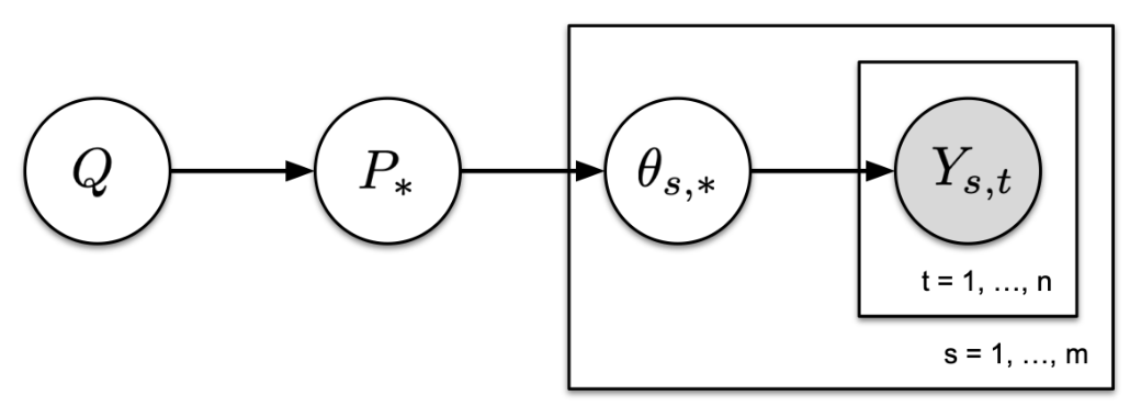
Refer to caption
Figure 1: Graphical model of our bandit environment.

Note that Thompson sampling requires P∗P_{*} as an input. In this work, we try to attain the same regret without assuming that P∗P_{*} is known. We formalize this problem in a Bayesian fashion. In particular, we assume the availability of a prior distribution QQ over problem instance priors, and that P∗∼QP_{*}\sim Q. We refer to QQ as a meta-prior since it is a prior over priors. In Bayesian statistics, this would also be known as a hyper-prior (Gelman et al. 2013). The agent knows QQ but not P∗P_{*}. We try to learn P∗P_{*} from sequential interactions with instances θs,∗\theta_{s,*}, which are drawn i.i.d. from P∗P_{*} in each task. Note that θs,∗\theta_{s,*} is also unknown. The agent only observes its noisy realizations Ys,tY_{s,t}. We visualize relations of QQ, P∗P_{*}, θs,∗\theta_{s,*}, and Ys,tY_{s,t} in a graphical model in Figure 1.

One motivating example for using a meta-prior for exploration arises in recommender systems, in which exploration is used to assess the latent interests of users for different items, such as movies. In this case, each user can be treated as a bandit instance where the items are arms. A standard prior over user latent interests could readily be used by TS (Hong et al. 2020). However, in many cases, the algorithm designer may be uncertain about its true form. For instance, the designer may believe that most users have strong but noisy affinity for items in exactly one of several classes, but it is unclear which. Our work can be viewed as formalizing the problem of learning such a prior over user interests, which could be used to start exploring the preferences of “cold-start” users.

3 Meta-Thompson Sampling

In this section, we present our approach to meta-learning in TS. We provide a general description in Section 3.1. In Sections 3.2 and 3.3, we implement it in Bernoulli bandits with a categorical meta-prior and Gaussian bandits with a Gaussian meta-prior, respectively. In Section 3.4, we justify our approach beyond these specific instances.

3.1 Algorithm 𝙼𝚎𝚝𝚊𝚃𝚂\tt MetaTS

Thompson sampling (Thompson 1933; Chapelle & Li 2012; Agrawal & Goyal 2012; Russo et al. 2018) is arguably the most popular and practical bandit algorithm. TS is parameterized by a prior, which is specified by the algorithm designer. In this work, we study a more general setting where the designer can model uncertainty over an unknown prior P∗P_{*} using a meta-prior QQ. Our proposed algorithm meta-learns P∗P_{*} from sequential interactions with bandit instances drawn i.i.d. from P∗P_{*}. Therefore, we call it meta-Thompson sampling (𝙼𝚎𝚝𝚊𝚃𝚂\tt MetaTS). In this subsection, we present 𝙼𝚎𝚝𝚊𝚃𝚂\tt MetaTS under the assumption that sample spaces are discrete. This eases exposition and guarantees that all conditional expectations are properly defined. We treat this topic more rigorously in Section 3.4.

𝙼𝚎𝚝𝚊𝚃𝚂\tt MetaTS is a variant of TS that models uncertainty over the instance prior distribution P∗P_{*}. This uncertainty is captured by a meta-posterior QsQ_{s}, a distribution over possible instance priors. We denote the meta-posterior in task ss by QsQ_{s}, and assume that each QsQ_{s} belongs to the same family as QQ. By definition, Q1=QQ_{1}=Q is the meta-prior. 𝙼𝚎𝚝𝚊𝚃𝚂\tt MetaTS samples the instance prior distribution PsP_{s} in task ss from QsQ_{s}. Then it applies TS with the sampled prior PsP_{s} to the bandit instance θs,∗\theta_{s,*} in task ss for nn rounds. Once the task is complete, it updates the meta-posterior in a standard Bayesian fashion

Qs+1​(P)\displaystyle Q_{s+1}(P) (1)
∝ℙ(H1:s|P∗=P)Q(P)\displaystyle\propto\mathbb{P}\left(H_{1:s}\,\middle|\,P_{*}=P\right)Q(P)
=ℙ⁡(Hs|P∗=P)​∏ℓ=1s−1ℙ⁡(Hℓ|P∗=P)​Q​(P)\displaystyle=\mathbb{P}\left(H_{s}\,\middle|\,P_{*}=P\right)\prod_{\ell=1}^{s-1}\mathbb{P}\left(H_{\ell}\,\middle|\,P_{*}=P\right)Q(P)
=ℙ⁡(Hs|P∗=P)​Qs​(P)\displaystyle=\mathbb{P}\left(H_{s}\,\middle|\,P_{*}=P\right)Q_{s}(P)
=∫θℙ⁡(Hs|θs,∗=θ)​ℙ​(θs,∗=θ|P∗=P)​⁡d​θ​Qs​(P),\displaystyle=\int_{\theta}\mathbb{P}\left(H_{s}\,\middle|\,\theta_{s,*}=\theta\right)\mathbb{P}\left(\theta_{s,*}=\theta\,\middle|\,P_{*}=P\right)\mathop{}\!\mathrm{d}\theta\,Q_{s}(P)\,,

where ℙ⁡(Hs|P∗=P)\mathbb{P}\left(H_{s}\,\middle|\,P_{*}=P\right) and ℙ⁡(Hs|θs,∗=θ)\mathbb{P}\left(H_{s}\,\middle|\,\theta_{s,*}=\theta\right) are probabilities of observations in task ss given that the instance prior is PP and the problem instance is θ\theta, respectively. A rigorous justification of this update is given in Section 3.4. Specific instances of this update are in Sections 3.2 and 3.3.

The pseudocode for 𝙼𝚎𝚝𝚊𝚃𝚂\tt MetaTS is presented in Algorithm 1. The algorithm is simple, natural, and general; but has two potential shortcomings. First, it is unclear if it can be implemented efficiently. To address this, we develop efficient implementations for both Bernoulli and Gaussian bandits in Sections 3.2 and 3.3, respectively. Second, it is unclear whether 𝙼𝚎𝚝𝚊𝚃𝚂\tt MetaTS explores enough. Ideally, it should learn to perform as well as TS with the true prior P∗P_{*}. Intuitively, we expect this since the meta-posterior samples Ps∼QsP_{s}\sim Q_{s} should vary significantly in the direction of high variance in QsQ_{s}, which represents high uncertainty that can be reduced by exploring. We confirm this in Section 4, where 𝙼𝚎𝚝𝚊𝚃𝚂\tt MetaTS is analyzed in Gaussian bandits.

Algorithm 1 𝙼𝚎𝚝𝚊𝚃𝚂\tt MetaTS: Meta-learning Thompson sampling.
Inputs:\Statex\State Meta-prior QQQ1←QQ_{1}\leftarrow Qs=1,…,ms=1,\dots,m Sample Ps∼QsP_{s}\sim Q_{s} Apply Thompson sampling with prior PsP_{s} to    problem instance θs,∗∼P∗\theta_{s,*}\sim P_{*} for nn rounds Update meta-posterior Qs+1Q_{s+1} , as defined in ( \EndFor )
\State
\Statex\State\For\State\State

3.2 Bernoulli Bandit with a Categorical Meta-Prior

Bernoulli Thompson sampling was the first instance of TS that was analyzed (Agrawal & Goyal 2012). In this section, we apply 𝙼𝚎𝚝𝚊𝚃𝚂\tt MetaTS to this problem class.

We consider a Bernoulli bandit with KK arms that is parameterized by arm means θ∈[0,1]K\theta\in[0,1]^{K}. The reward of arm ii in instance θ\theta is drawn i.i.d. from Ber⁡(θi)\mathrm{Ber}(\theta_{i}). To model uncertainty in the prior, we assume access to LL potential instance priors 𝒫={P(j)}j=1L\mathcal{P}=\left\{P^{(j)}\right\}_{j=1}^{L}. Each prior P(j)P^{(j)} is factored across the arms as

P(j)​(θ)\displaystyle P^{(j)}(\theta) =∏i=1KBeta⁡(θi,αi,j,βi,j)\displaystyle=\prod_{i=1}^{K}\mathrm{Beta}(\theta_{i};\alpha_{i,j},\beta_{i,j})
=∏i=1KΓ⁡(αi,j+βi,j)Γ⁡(αi,j)​Γ​(βi,j)​θiαi,j−1​(1−θi)βi,j−1\displaystyle=\prod_{i=1}^{K}\frac{\Gamma(\alpha_{i,j}+\beta_{i,j})}{\Gamma(\alpha_{i,j})\Gamma(\beta_{i,j})}\theta_{i}^{\alpha_{i,j}-1}(1-\theta_{i})^{\beta_{i,j}-1}

for some fixed (αi,j)i=1K(\alpha_{i,j})_{i=1}^{K} and (βi,j)i=1K(\beta_{i,j})_{i=1}^{K}. The meta-prior is a categorical distribution over LL classes of tasks. That is,

Q⁡(j)=Cat⁡(j,w)=wj\displaystyle Q(j)=\mathrm{Cat}(j;w)=w_{j}

for w∈ΔL−1w\in\Delta_{L-1}, where ww is a vector of initial beliefs into each instance prior and ΔL−1\Delta_{L-1} is the LL-dimensional simplex. The tasks are generated as follows. First, the instance prior is set as P∗=P(j∗)P_{*}=P^{(j_{*})} where j∗∼Qj_{*}\sim Q. Then, in each task ss, a Bernoulli bandit instance is sampled as θs,∗∼P∗\theta_{s,*}\sim P_{*}.

𝙼𝚎𝚝𝚊𝚃𝚂\tt MetaTS is implemented as follows. The meta-posterior in task ss is

Qs​(j)=Cat⁡(j,w^s)=w^s,j,\displaystyle Q_{s}(j)=\mathrm{Cat}(j;\hat{w}_{s})=\hat{w}_{s,j}\,,

where w^s∈ΔL−1\hat{w}_{s}\in\Delta_{L-1} is a vector of posterior beliefs into each instance prior. The instance prior in task ss is Ps=P(js)P_{s}=P^{(j_{s})} where js∼Qsj_{s}\sim Q_{s}. After interacting with bandit instance θs,∗\theta_{s,*}, the meta-posterior is updated using Qs+1​(j)∝f⁡(j)​Qs​(j)Q_{s+1}(j)\propto f(j)\,Q_{s}(j), where

f⁡(j)=\displaystyle f(j)={} ∫θℙ⁡(Hs|θs,∗=θ)​ℙ​(θs,∗=θ|j∗=j)​⁡𝑑θ\displaystyle\int_{\theta}\mathbb{P}\left(H_{s}\,\middle|\,\theta_{s,*}=\theta\right)\mathbb{P}\left(\theta_{s,*}=\theta\,\middle|\,j_{*}=j\right)\mathop{}\!\mathrm{d}\theta
=\displaystyle={} ∏i=1KΓ⁡(αi,j+βi,j)Γ⁡(αi,j)​Γ​(βi,j)×\displaystyle\prod_{i=1}^{K}\frac{\Gamma(\alpha_{i,j}+\beta_{i,j})}{\Gamma(\alpha_{i,j})\Gamma(\beta_{i,j})}\times{}
∫θiθiαi,j+Ni,s+−1​(1−θi)βi,j+Ni,s−−1​⁡d​θi\displaystyle\int_{\theta_{i}}\theta_{i}^{\alpha_{i,j}+N_{i,s}^{+}-1}(1-\theta_{i})^{\beta_{i,j}+N_{i,s}^{-}-1}\mathop{}\!\mathrm{d}\theta_{i}
=\displaystyle={} ∏i=1KΓ⁡(αi,j+βi,j)​Γ​(αi,j+Ni,s+)​Γ​(βi,j+Ni,s−)Γ⁡(αi,j)​Γ​(βi,j)​Γ​(αi,j+βi,j+Ti,s).\displaystyle\prod_{i=1}^{K}\frac{\Gamma(\alpha_{i,j}+\beta_{i,j})\Gamma(\alpha_{i,j}+N_{i,s}^{+})\Gamma(\beta_{i,j}+N_{i,s}^{-})}{\Gamma(\alpha_{i,j})\Gamma(\beta_{i,j})\Gamma(\alpha_{i,j}+\beta_{i,j}+T_{i,s})}\,.

Here 𝒜i,s={t∈[n]:As,t=i}\mathcal{A}_{i,s}=\left\{t\in[n]:A_{s,t}=i\right\} is the set of rounds where arm ii is pulled in task ss and Ti,s=|𝒜i,s|T_{i,s}=\left|\mathcal{A}_{i,s}\right| is the number of these rounds. In addition, Ni,s+=∑t∈𝒜i,sYs,t​(i)N_{i,s}^{+}=\sum_{t\in\mathcal{A}_{i,s}}Y_{s,t}(i) denotes the number of positive observations of arm ii and Ni,s−=Ti,s−Ni,s+N_{i,s}^{-}=T_{i,s}-N_{i,s}^{+} is the number of its negative observations.

The above derivation can be generalized in a straightforward fashion to any categorical meta-prior whose instance priors P(j)P^{(j)} lie in some exponential family.

3.3 Gaussian Bandit with a Gaussian Meta-Prior

Gaussian distributions have many properties that allow for tractable analysis, such as that the posterior variance is independent of observations, which we exploit in Section 4. In this section, we present a computationally-efficient implementation for this problem class.

We consider a Gaussian bandit with KK arms that is parameterized by arm means θ∈ℝK\theta\in\mathbb{R}^{K}. The reward of arm ii in instance θ\theta is drawn i.i.d. from 𝒩⁡(θi,σ2)\mathcal{N}(\theta_{i},\sigma^{2}). We have a continuum of instance priors, parameterized by a vector of means μ∈ℝK\mu\in\mathbb{R}^{K} and defined as P⁡(θ)=𝒩⁡(θ,μ,σ02​IK)P(\theta)=\mathcal{N}(\theta;\mu,\sigma_{0}^{2}I_{K}). The noise σ0\sigma_{0} is fixed. The meta-prior is a Gaussian distribution over instance prior means Q⁡(μ)=𝒩⁡(μ,𝟎,σq2​IK)Q(\mu)=\mathcal{N}(\mu;\mathbf{0},\sigma_{q}^{2}I_{K}), where σq\sigma_{q} is assumed to be known. The tasks are generated as follows. First, the instance prior is set as P∗=𝒩⁡(μ∗,σ02​IK)P_{*}=\mathcal{N}(\mu_{*},\sigma_{0}^{2}I_{K}) where μ∗∼Q\mu_{*}\sim Q. Then, in each task ss, a Gaussian bandit instance is sampled as θs,∗∼P∗\theta_{s,*}\sim P_{*}.

𝙼𝚎𝚝𝚊𝚃𝚂\tt MetaTS is implemented as follows. The meta-posterior in task ss is

Qs​(μ)=𝒩⁡(μ,μ^s,Σ^s),\displaystyle Q_{s}(\mu)=\mathcal{N}(\mu;\hat{\mu}_{s},\hat{\Sigma}_{s})\,,

where μ^s∈ℝK\hat{\mu}_{s}\in\mathbb{R}^{K} is an estimate of μ∗\mu_{*} and Σ^s∈ℝK×K\hat{\Sigma}_{s}\in\mathbb{R}^{K\times K} is a diagonal covariance matrix. The instance prior in task ss is Ps​(θ)=𝒩⁡(θ,μ~s,σ02​IK)P_{s}(\theta)=\mathcal{N}(\theta;\tilde{\mu}_{s},\sigma_{0}^{2}I_{K}) where μ~s∼Qs\tilde{\mu}_{s}\sim Q_{s}. After interacting with bandit instance θs,∗\theta_{s,*}, the meta-posterior is updated as Qs+1​(μ)∝f⁡(μ)​Qs​(μ)Q_{s+1}(\mu)\propto f(\mu)\,Q_{s}(\mu), where

f⁡(μ)\displaystyle f(\mu)
=∫θℙ⁡(Hs|θs,∗=θ)​ℙ​(θs,∗=θ|μ∗=μ)​⁡𝑑θ\displaystyle=\int_{\theta}\mathbb{P}\left(H_{s}\,\middle|\,\theta_{s,*}=\theta\right)\mathbb{P}\left(\theta_{s,*}=\theta\,\middle|\,\mu_{*}=\mu\right)\mathop{}\!\mathrm{d}\theta
=∏i=1K∫θi[∏t∈𝒜i,s𝒩⁡(Ys,t​(i),θi,σ2)]​𝒩​(θi,μi,σ02)​⁡d​θi.\displaystyle=\prod_{i=1}^{K}\int_{\theta_{i}}\left[\prod_{t\in\mathcal{A}_{i,s}}\mathcal{N}(Y_{s,t}(i);\theta_{i},\sigma^{2})\right]\mathcal{N}(\theta_{i};\mu_{i},\sigma_{0}^{2})\mathop{}\!\mathrm{d}\theta_{i}\,.

Here 𝒜i,s={t∈[n]:As,t=i}\mathcal{A}_{i,s}=\left\{t\in[n]:A_{s,t}=i\right\} is the set of rounds where arm ii is pulled in task ss and Ti,s=|𝒜i,s|T_{i,s}=\left|\mathcal{A}_{i,s}\right| is the number of such rounds, as in Section 3.2.

Since Σ^s=diag⁡(σ^s2)\hat{\Sigma}_{s}=\mathrm{diag}\left(\hat{\sigma}_{s}^{2}\right) is a diagonal covariance matrix, it is fully characterized by a vector of individual arm variances σ^s2∈ℝK\hat{\sigma}_{s}^{2}\in\mathbb{R}^{K}. The parameters μ^s\hat{\mu}_{s} and σ^s2\hat{\sigma}_{s}^{2} are updated, based on Lemma 7 in Appendix B, as

μ^s+1,i\displaystyle\hat{\mu}_{s+1,i} =σ^s+1,i2​(μ^s,iσ^s,i2+Ti,sTi,s​σ02+σ2​∑t∈𝒜i,sYs,t​(i)Ti,s),\displaystyle=\hat{\sigma}_{s+1,i}^{2}\left(\frac{\hat{\mu}_{s,i}}{\hat{\sigma}_{s,i}^{2}}+\frac{T_{i,s}}{T_{i,s}\sigma_{0}^{2}+\sigma^{2}}\frac{\sum_{t\in\mathcal{A}_{i,s}}Y_{s,t}(i)}{T_{i,s}}\right)\,,
σ^s+1,i−2\displaystyle\hat{\sigma}_{s+1,i}^{-2} =σ^s,i−2+Ti,sTi,s​σ02+σ2.\displaystyle=\hat{\sigma}_{s,i}^{-2}+\frac{T_{i,s}}{T_{i,s}\sigma_{0}^{2}+\sigma^{2}}\,.

This update can be also derived using (17) in Appendix D, when all covariance matrices are assumed to be diagonal.

The above update has a very nice interpretation. The posterior mean μ^s+1,i\hat{\mu}_{s+1,i} of arm ii is a weighted sum of the mean reward estimate of arm ii in task ss and the earlier posterior mean μ^s,i\hat{\mu}_{s,i}. The weight of the estimate depends on how good it is. Specifically, it varies from 1/(σ0,i2+σ2)1/(\sigma_{0,i}^{2}+\sigma^{2}), when arm ii is pulled only once, to 1/σ0,i21/\sigma_{0,i}^{2}, when Ti,s→∞T_{i,s}\to\infty. This is the minimum amount of uncertainty that cannot be reduced by more pulls, due to the fact that θs,∗\theta_{s,*} is a single observation of the unknown μ∗\mu_{*} with covariance σ02​IK\sigma_{0}^{2}I_{K}.

3.4 Measure-Theoretic View and the General Case

We now present a more general measure-theoretic specification of our meta-bandit setting. Let 𝒵\mathcal{Z} be the set of outcomes for the hidden variable ZZ that is sampled from a meta-prior and σ⁡(𝒵)\sigma(\mathcal{Z}) be the σ\sigma-algebra over this set. Similarly, let Θ\Theta be the set of possible bandit environments θ∈Θ\theta\in\Theta and σ⁡(Θ)\sigma(\Theta) be the σ\sigma-algebra over this set. While in this work we focus on environments characterized only by their mean reward vectors, this parameterization could be more general, and for example include the variance of mean reward vectors. The formal definition of a KK-armed Bayesian meta-bandit is as follows.

Definition 1.

A KK-armed Bayesian meta-bandit is a tuple ℬ=(𝒵,σ⁡(𝒵),Q,Θ,σ⁡(Θ),P,ρ)\mathcal{B}=(\mathcal{Z},\sigma(\mathcal{Z}),Q,\Theta,\sigma(\Theta),P,\rho), where (𝒵,σ⁡(𝒵))(\mathcal{Z},\sigma(\mathcal{Z})) is a measurable space; the meta-prior QQ is a probability measure over (𝒵,σ⁡(𝒵))(\mathcal{Z},\sigma(\mathcal{Z})); the prior PP is a probability kernel from (𝒵,σ⁡(𝒵))(\mathcal{Z},\sigma(\mathcal{Z})) to (Θ,σ⁡(Θ))(\Theta,\sigma(\Theta)); and ρ=(ρθ,i:θ∈Θ,i∈[K])\rho=(\rho_{\theta,i}:\theta\in\Theta,i\in[K]) is a probability kernel from Θ×[K]\Theta\times[K] to (ℝ,𝔅⁡(ℝ))(\mathbb{R},\mathfrak{B}(\mathbb{R})), where 𝔅⁡(ℝ)\mathfrak{B}(\mathbb{R}) is the Borel σ\sigma-algebra of ℝ\mathbb{R} and ρθ,i\rho_{\theta,i} is the reward distribution associated with arm ii in bandit θ\theta.

We use lowercase letters to denote realizations of random variables. Let PzP_{z} be a distribution of bandit instances under Z=zZ=z. We assume that a new environment θ∈Θ\theta\in\Theta is sampled from the same measure PzP_{z} at the beginning of each task with the same realization of hidden variable ZZ sampled from the meta-prior QQ beforehand.

A bandit algorithm consists of kernels πs,t\pi_{s,t} that take as input a history of interactions consisting of the pulled arms and observed rewards up to round tt in task ss, and output a probability measure over the arms. A bandit algorithm is connected with a Bayesian meta-bandit environment ℬ\mathcal{B} to produce a sequence of chosen arms and observed rewards. Formally, let Ωs,t=([K]×ℝ)(s−1)​n+t−1⊂ℝ2​((s−1)​n+t−1)\Omega_{s,t}=([K]\times\mathbb{R})^{(s-1)n+t-1}\subset\mathbb{R}^{2((s-1)n+t-1)} for each t∈[n]t\in[n] and s∈[m]s\in[m]. Then a bandit algorithm or policy is a tuple π=(πs,t)s,t=1m,n\pi=(\pi_{s,t})_{s,t=1}^{m,n} such that each πs,t\pi_{s,t} is a kernel from (Ωs,t,𝔅⁡(ℝ2​((s−1)​n+t−1)))(\Omega_{s,t},\mathfrak{B}(\mathbb{R}^{2((s-1)n+t-1)})) to ([K],2[K])([K],2^{[K]}) that interacts with a Bayesian meta-bandit ℬ\mathcal{B} over mm tasks, each lasting nn rounds and producing a sequence of random variables

A1,1,X1,1,…,A1,n,X1,n,…,\displaystyle A_{1,1},X_{1,1},\dots,A_{1,n},X_{1,n}\,,\dots,
Am,1,Xm,1​…,Am,n,Xm,n,\displaystyle A_{m,1},X_{m,1}\dots,A_{m,n},X_{m,n}\,,

where Xs,t=Ys,t​(As,t)X_{s,t}=Y_{s,t}(A_{s,t}) is the reward in round tt of task ss. The probability measure over these variables, ℙz,θ1,…,θm,π\mathbb{P}_{z,\theta_{1},\dots,\theta_{m},\pi}, is guaranteed to exist by the Ionescu-Tulcea theorem (Tulcea 1949). Furthermore, the conditional probabilities of transitions of this measure are equal to the kernels

ℙ(θs∈⋅|z,θ1,…,θs−1,H1:s−1)=Pz(θs∈⋅),\displaystyle\mathbb{P}\left(\theta_{s}\in\cdot\,\middle|\,z,\theta_{1},\dots,\theta_{s-1},H_{1:s-1}\right)=P_{z}(\theta_{s}\in\cdot)\,,
ℙ(As,t∈⋅|z,θ1,…,θs,H1:s−1,Hs,t)=\displaystyle\mathbb{P}\left(A_{s,t}\in\cdot\,\middle|\,z,\theta_{1},\dots,\theta_{s},H_{1:s-1},H_{s,t}\right)=
πs,t(As,t∈⋅|H1:s−1,Hs,t),\displaystyle\qquad\pi_{s,t}(A_{s,t}\in\cdot\,|\,H_{1:s-1},H_{s,t})\,,
ℙ(Xs,t∈⋅|z,θ1,…,θs,H1:s−1,Hs,t,As,t)=\displaystyle\mathbb{P}\left(X_{s,t}\in\cdot\,\middle|\,z,\theta_{1},\dots,\theta_{s},H_{1:s-1},H_{s,t},A_{s,t}\right)=
ρθs,As,t(Xs,t∈⋅),\displaystyle\qquad\rho_{\theta_{s},A_{s,t}}(X_{s,t}\in\cdot)\,,

where Hs,t=(Xs,ℓ,As,ℓ)ℓ=1t−1H_{s,t}=(X_{s,\ell},A_{s,\ell})_{\ell=1}^{t-1}. The following lemma says that both the task-posterior Pz(⋅|hs,t)P_{z}(\cdot|h_{s,t}) for any z∈𝒵z\in\mathcal{Z} and the meta-posterior Q(⋅|h1:s−1)Q(\cdot|h_{1:s-1}) depend only on the pulled arms according to π\pi, but not the exact form of π\pi.

Lemma 2.

Assume that there exists a σ\sigma-finite measure λρ\lambda_{\rho} on (ℝ,𝔅⁡(ℝ))(\mathbb{R},\mathfrak{B}(\mathbb{R})) such that ρθ,i\rho_{\theta,i} is absolutely continuous with respect to λρ\lambda_{\rho} for all θ∈Θ\theta\in\Theta and i∈[K]i\in[K]. Then the task-posterior and meta-posterior exist and have the following form

Pz​(S1|hs,t)=∫S1∏j=1t−1pθs,as,j​(xs,j)​⁡d​Pz​(θs)∫Θ∏j=1t−1pθs,as,j​(xs,j)​⁡d​Pz​(θs),\displaystyle P_{z}(S_{1}|h_{s,t})=\frac{\int_{S_{1}}\prod_{j=1}^{t-1}p_{\theta_{s},a_{s,j}}(x_{s,j})\mathop{}\!\mathrm{d}P_{z}(\theta_{s})}{\int_{\Theta}\prod_{j=1}^{t-1}p_{\theta_{s},a_{s,j}}(x_{s,j})\mathop{}\!\mathrm{d}P_{z}(\theta_{s})},
Q(S2|h1:s−1)=\displaystyle Q(S_{2}|h_{1:s-1})=
∫S2[∏ℓ=1s−1∏j=1n∫Θpθ,aℓ,j​(xℓ,j)​⁡d​Pz​(θ)]​⁡d​Q​(z)∫𝒵[∏ℓ=1s−1∏j=1n∫Θpθ,aℓ,j​(xℓ,j)​⁡d​Pz​(θ)]​⁡d​Q​(z),\displaystyle\quad\frac{\int_{S_{2}}\left[\prod_{\ell=1}^{s-1}\prod_{j=1}^{n}\int_{\Theta}p_{\theta,a_{\ell,j}}(x_{\ell,j})\mathop{}\!\mathrm{d}P_{z}(\theta)\right]\mathop{}\!\mathrm{d}Q(z)}{\int_{\mathcal{Z}}\left[\prod_{\ell=1}^{s-1}\prod_{j=1}^{n}\int_{\Theta}p_{\theta,a_{\ell,j}}(x_{\ell,j})\mathop{}\!\mathrm{d}P_{z}(\theta)\right]\mathop{}\!\mathrm{d}Q(z)},

for any S1∈σ⁡(Θ),z∈𝒵,S2∈σ⁡(𝒵)S_{1}\in\sigma(\Theta),z\in\mathcal{Z},S_{2}\in\sigma(\mathcal{Z}).

The proof is provided in Appendix C. 𝙼𝚎𝚝𝚊𝚃𝚂\tt MetaTS samples ZsZ_{s} from the meta-posterior Qs=Q(⋅|h1:s−1)Q_{s}=Q(\cdot|h_{1:s-1}) at the beginning of each task s∈[m]s\in[m] and then pulls arms according to the samples from PZs(⋅|hs,t)P_{Z_{s}}(\cdot|h_{s,t}). The above lemma shows that to compute the posteriors we only need the distributions of rewards and integrate them over the environments (for the task-posterior) or over both the environments and the hidden variables (for the meta-posterior).These integrals can be derived analytically, for example, in the case of conjugate priors Sections 3.3 and 3.2.

4 Analysis

We bound the Bayes regret of 𝙼𝚎𝚝𝚊𝚃𝚂\tt MetaTS in Gaussian bandits (Section 3.3). This section is organized as follows. We state the bound and sketch its proof in Section 4.1, and discuss it in Section 4.2. In Section 4.3, we present the key lemmas. Finally, in Section 4.4, we discuss how our analysis can be extended beyond Gaussian bandits.

4.1 Regret Bound

We analyze 𝙼𝚎𝚝𝚊𝚃𝚂\tt MetaTS under the assumption that each arm is pulled at least once per task. Although this suffices to show benefits of meta-learning, it is conservative. A less conservative analysis would require understanding how Thompson sampling with a misspecified prior pulls arms. In particular, we would require a high-probability lower bound on the number of pulls of each arm. To the best of our knowledge, such as a bound does not exist and is non-trivial to derive. To guarantee that each arm is pulled at least once, we pull each arm in the last KK rounds of each task. This is to avoid any interference with our posterior sampling analyses in the earlier rounds. Other than this, 𝙼𝚎𝚝𝚊𝚃𝚂\tt MetaTS is analyzed exactly as described in Sections 3.1 and 3.3.

Recall the following definitions in our setting (Section 3.3). The meta-prior is Q=𝒩⁡(𝟎,σq2​IK)Q=\mathcal{N}(\mathbf{0},\sigma_{q}^{2}I_{K}). The instance prior is P∗=𝒩⁡(μ∗,σ02​IK)P_{*}=\mathcal{N}(\mu_{*},\sigma_{0}^{2}I_{K}), where μ∗∼Q\mu_{*}\sim Q is chosen before the learning agent interact with the tasks. Then, in each task ss, a problem instance is drawn i.i.d. as θs,∗∼P∗\theta_{s,*}\sim P_{*}. Our main result is the following Bayes regret bound.

Theorem 3.

The Bayes regret of 𝙼𝚎𝚝𝚊𝚃𝚂\tt MetaTS over mm tasks with nn rounds each is

R⁡(m,n,P∗)≤\displaystyle R(m,n;P_{*})\leq
c1​K​(n+σ2​σ0−2​K−σ2​σ0−2​K)​m+\displaystyle\quad c_{1}\sqrt{K}\left(\sqrt{n+\sigma^{2}\sigma_{0}^{-2}K}-\sqrt{\sigma^{2}\sigma_{0}^{-2}K}\right)m+{}
c2​(δ)​c3​(δ)​K​n2​m+O~​(K​m+n)\displaystyle\quad c_{2}(\delta)c_{3}(\delta)Kn^{2}\sqrt{m}+\tilde{O}(Km+n)

with probability at least 1−(2​m+1)​δ1-(2m+1)\delta, where

c1\displaystyle c_{1} =4​2​σ2​log⁡n,\displaystyle=4\sqrt{2\sigma^{2}\log n}\,,
c2​(δ)\displaystyle c_{2}(\delta) =2​(2​σq2​log⁡(2​K/δ)+2​σ02​log⁡n),\displaystyle=2\left(\sqrt{2\sigma_{q}^{2}\log(2K/\delta)}+\sqrt{2\sigma_{0}^{2}\log n}\right)\,,
c3​(δ)\displaystyle c_{3}(\delta) =8​(σ02+σ2)​log⁡(4​K/δ)/(π​σ02).\displaystyle=8\sqrt{(\sigma_{0}^{2}+\sigma^{2})\log(4K/\delta)/(\pi\sigma_{0}^{2})}\,.

The probability is over realizations of μ∗\mu_{*}, θs,∗\theta_{s,*}, and μ^s\hat{\mu}_{s}.

Proof.

First, we bound the magnitude of μ∗\mu_{*}. Specifically, since μ∗∼𝒩⁡(𝟎,σq2​IK)\mu_{*}\sim\mathcal{N}(\mathbf{0},\sigma_{q}^{2}I_{K}), we have that

‖μ∗‖∞≤2​σq2​log⁡(2​K/δ)\displaystyle\|\mu_{*}\|_{\infty}\leq\sqrt{2\sigma_{q}^{2}\log(2K/\delta)} (2)

holds with probability at least 1−δ1-\delta.

Now we fix task s≥2s\geq 2 and decompose its regret. Let As,∗A_{s,*} be the optimal arm in instance θs,∗\theta_{s,*}, As,tA_{s,t} be the pulled arm in round tt by TS with misspecified prior PsP_{s}, and A~s,t\tilde{A}_{s,t} be the pulled arm in round tt by TS with correct prior P∗P_{*}. Then

𝔼⁡[∑t=1nθs,∗​(As,∗)−θs,∗​(As,t)|P∗]=Rs,1+Rs,2,\displaystyle\mathbb{E}\left[\sum_{t=1}^{n}\theta_{s,*}(A_{s,*})-\theta_{s,*}(A_{s,t})\,\middle|\,P_{*}\right]=R_{s,1}+R_{s,2}\,,

where

Rs,1\displaystyle R_{s,1} =𝔼⁡[∑t=1nθs,∗​(As,∗)−θs,∗​(A~s,t)|P∗],\displaystyle=\mathbb{E}\left[\sum_{t=1}^{n}\theta_{s,*}(A_{s,*})-\theta_{s,*}(\tilde{A}_{s,t})\,\middle|\,P_{*}\right]\,,
Rs,2\displaystyle R_{s,2} =𝔼⁡[∑t=1nθs,∗​(A~s,t)−θs,∗​(As,t)|P∗].\displaystyle=\mathbb{E}\left[\sum_{t=1}^{n}\theta_{s,*}(\tilde{A}_{s,t})-\theta_{s,*}(A_{s,t})\,\middle|\,P_{*}\right]\,.

The term Rs,1R_{s,1} is the regret of hypothetical TS that knows P∗P_{*}. This TS is introduced only for the purpose of analysis and is the optimal policy. The term Rs,2R_{s,2} is the difference in the expected nn-round rewards of TS with priors PsP_{s} and P∗P_{*}, and vanishes as the number of tasks ss increases.

To bound Rs,1R_{s,1}, we apply Lemma 4 with δ=1/n\delta=1/n and get

Rs,1≤\displaystyle R_{s,1}\leq{} 42​σ2​K​log⁡n×\displaystyle 4\sqrt{2\sigma^{2}K\log n}\times{}
(n+σ2​σ0−2​K−σ2​σ0−2​K)+O~​(K),\displaystyle\left(\sqrt{n+\sigma^{2}\sigma_{0}^{-2}K}-\sqrt{\sigma^{2}\sigma_{0}^{-2}K}\right)+\tilde{O}(K)\,,

where O~​(K)\tilde{O}(K) corresponds to the c⁡(δ)c(\delta) term in Lemma 4. To bound Rs,2R_{s,2}, we apply Lemma 5 with δ=1/n\delta=1/n and get

Rs,2≤\displaystyle R_{s,2}\leq{} 2(∥μ∗∥∞+2​σ02​log⁡n)2π​σ02×\displaystyle 2\left(\|\mu_{*}\|_{\infty}+\sqrt{2\sigma_{0}^{2}\log n}\right)\sqrt{\frac{2}{\pi\sigma_{0}^{2}}}\times{}
K​n2​‖μ~s−μ∗‖∞+O~​(K),\displaystyle Kn^{2}\|\tilde{\mu}_{s}-\mu_{*}\|_{\infty}+\tilde{O}(K)\,,

where O~​(K)\tilde{O}(K) is the first term in Lemma 5, after we bound ‖μ∗‖∞\|\mu_{*}\|_{\infty} in it using (2).

Now we sum up our bounds on Rs,1+Rs,2R_{s,1}+R_{s,2} over all tasks s≥2s\geq 2 and get

c1​K​(n+σ2​σ0−2​K−σ2​σ0−2​K)​m+\displaystyle c_{1}\sqrt{K}\left(\sqrt{n+\sigma^{2}\sigma_{0}^{-2}K}-\sqrt{\sigma^{2}\sigma_{0}^{-2}K}\right)m+{}
c2​(δ)​2π​σ02​K​n2​∑s=2m‖μ~s−μ∗‖∞+O~​(K​m),\displaystyle c_{2}(\delta)\sqrt{\frac{2}{\pi\sigma_{0}^{2}}}Kn^{2}\sum_{s=2}^{m}\|\tilde{\mu}_{s}-\mu_{*}\|_{\infty}+\tilde{O}(Km)\,,

where c1c_{1} and c2​(δ)c_{2}(\delta) are defined in the main claim. Then we apply Lemma 6 to each term ‖μ~s−μ∗‖∞\|\tilde{\mu}_{s}-\mu_{*}\|_{\infty} and have with probability at least 1−m​δ1-m\delta that

∑s=2m‖μ~s−μ∗‖∞≤4​2​(σ02+σ2)​m​log⁡(4​K/δ),\displaystyle\sum_{s=2}^{m}\|\tilde{\mu}_{s}-\mu_{*}\|_{\infty}\leq 4\sqrt{2(\sigma_{0}^{2}+\sigma^{2})m\log(4K/\delta)}\,,

where m\sqrt{m} arises from summing up the O⁡(1/s)O(1/\sqrt{s}) terms in Lemma 6, using Lemma 8 in Appendix B. This concludes the main part of the proof.

We finish with an upper bound on the regret in task 11 and the cost of pulling each arm once at the end of each task. This is can done as follows. Since θs,∗∼𝒩⁡(μ∗,σ02​IK)\theta_{s,*}\sim\mathcal{N}(\mu_{*},\sigma_{0}^{2}I_{K}),

‖θs,∗−μ∗‖∞≤2​σ02​log⁡(2​K/δ)\displaystyle\|\theta_{s,*}-\mu_{*}\|_{\infty}\leq\sqrt{2\sigma_{0}^{2}\log(2K/\delta)} (3)

holds with probability at least 1−δ1-\delta in any task ss. From (2) and (3), we have with a high probability that

‖θs,∗‖∞\displaystyle\|\theta_{s,*}\|_{\infty} ≤‖θs,∗−μ∗‖∞+‖μ∗‖∞\displaystyle\leq\|\theta_{s,*}-\mu_{*}\|_{\infty}+\|\mu_{*}\|_{\infty}
≤2​(σq2+σ02)​log⁡(2​K/δ).\displaystyle\leq 2\sqrt{(\sigma_{q}^{2}+\sigma_{0}^{2})\log(2K/\delta)}\,.

This yields a high-probability upper bound of

4​(σq2+σ02)​log⁡(2​K/δ)​(n+K​m)\displaystyle 4\sqrt{(\sigma_{q}^{2}+\sigma_{0}^{2})\log(2K/\delta)}(n+Km)

on the regret in task 11 and pulling each arm once at the end of all tasks. This concludes our proof. ∎

4.2 Discussion

If we assume a “large mm and nn” regime, where the learning agent improves with more tasks but also needs to perform well in each task, the most important terms in Theorem 3 are those where mm and nn interact. Using these terms, our bound can be summarized as

K​[n+σ2​σ0−2​K−σ2​σ0−2​K]​m+K​n2​m\displaystyle\!\!\!\!\!\!\sqrt{K}\left[\sqrt{n+\sigma^{2}\sigma_{0}^{-2}K}-\sqrt{\sigma^{2}\sigma_{0}^{-2}K}\right]m+Kn^{2}\sqrt{m} (4)

and holds with probability 1−(2​m+1)​δ1-(2m+1)\delta for any δ>0\delta>0.

Our bound in (4) can be viewed as follows. The first term is the regret of Thompson sampling with the correct prior P∗P_{*}. It is linear in the number of tasks mm, since 𝙼𝚎𝚝𝚊𝚃𝚂\tt MetaTS solves mm exploration problems. The second term captures the cost of learning P∗P_{*}. Since it is sublinear in the number of tasks mm, 𝙼𝚎𝚝𝚊𝚃𝚂\tt MetaTS is near optimal in the regime of “large mm”.

We compare our bound to two baselines. The first baseline is TS with a known prior P∗P_{*}. The regret of this TS can be bounded using Lemma 4 and includes only the first term in (4). In the regime of “large m”, this term dominates the regret of 𝙼𝚎𝚝𝚊𝚃𝚂\tt MetaTS, and thus 𝙼𝚎𝚝𝚊𝚃𝚂\tt MetaTS is near optimal.

The second baseline is agnostic Thompson sampling, which does use the structure θs,∗∼P∗∼Q\theta_{s,*}\sim P_{*}\sim Q. Instead, it marginalizes out QQ. In our setting, this can be equivalently viewed as assuming θs,∗∼𝒩⁡(𝟎,(σq2+σ02)​IK)\theta_{s,*}\sim\mathcal{N}(\mathbf{0},(\sigma_{q}^{2}+\sigma_{0}^{2})I_{K}). For this prior, the Bayes regret is 𝔼⁡[R⁡(m,n,P∗)]\mathbb{E}\left[R(m,n;P_{*})\right], where the expectation is over P∗∼QP_{*}\sim Q. Again, we can apply Lemma 4 and show that 𝔼⁡[R⁡(m,n,P∗)]\mathbb{E}\left[R(m,n;P_{*})\right] has an upper bound of

K​(n+σ2​σ~−1​K−σ2​σ~−1​K)​m,\displaystyle\sqrt{K}\left(\sqrt{n+\sigma^{2}\tilde{\sigma}^{-1}K}-\sqrt{\sigma^{2}\tilde{\sigma}^{-1}K}\right)m\,,

where σ~2=σq2+σ02\tilde{\sigma}^{2}=\sigma_{q}^{2}+\sigma_{0}^{2}. Clearly, σ~2>σ02\tilde{\sigma}^{2}>\sigma_{0}^{2}; and therefore the difference of the above square roots is always larger than in (4). So, in the regime of “large m”, 𝙼𝚎𝚝𝚊𝚃𝚂\tt MetaTS has a lower regret than this baseline.

4.3 Key Lemmas

Now we present the three key lemmas used in the proof of Theorem 3. They are proved in Appendix A.

The first lemma is a prior-dependent upper bound on the Bayes regret of TS.

Lemma 4.

Let θ∗\theta_{*} be arm means in a KK-armed Gaussian bandit that are generated as θ∗∼P∗=𝒩⁡(μ∗,σ02​IK)\theta_{*}\sim P_{*}=\mathcal{N}(\mu_{*},\sigma_{0}^{2}I_{K}). Let A∗A_{*} be the optimal arm under θ∗\theta_{*} and AtA_{t} be the pulled arm in round tt by TS with prior P∗P_{*}. Then for any δ>0\delta>0,

𝔼⁡[∑t=1nθ∗​(A∗)−θ∗​(At)]≤c⁡(δ)+\displaystyle\mathbb{E}\left[\sum_{t=1}^{n}\theta_{*}(A_{*})-\theta_{*}(A_{t})\right]\leq c(\delta)+{}
4​2​σ2​K​log⁡(1/δ)​(n+σ2​σ0−2​K−σ2​σ0−2​K),\displaystyle\quad 4\sqrt{2\sigma^{2}K\log(1/\delta)}\left(\sqrt{n+\sigma^{2}\sigma_{0}^{-2}K}-\sqrt{\sigma^{2}\sigma_{0}^{-2}K}\right)\,,

where c⁡(δ)=2​2​σ02​log⁡(1/δ)​K+2​σ02/π​K​n​δc(\delta)=2\sqrt{2\sigma_{0}^{2}\log(1/\delta)}K+\sqrt{2\sigma_{0}^{2}/\pi}Kn\delta.

The effect of the prior is reflected in the difference of the square roots. As the prior width narrows and σ0→0\sigma_{0}\to 0, the difference decreases, which shows that a more concentrated prior leads to less exploration. The algebraic form of the bound is also expected. Roughly speaking, σ2​σ0−2​K\sqrt{\sigma^{2}\sigma_{0}^{-2}K} is the sum of confidence interval widths in the Bayes regret analysis that cannot occur, because the prior width is σ0\sigma_{0}.

The bound in Lemma 4 differs from other similar bounds in the literature (Lu & Van Roy 2019). One difference is that the Cauchy-Schwarz inequality is not used in its proof. Therefore, σ0\sigma_{0} is in the square root instead of the logarithm. The resulting bound is tighter for σ2​σ0−2​K≪n\sigma^{2}\sigma_{0}^{-2}K\ll n. Another difference is that information-theory arguments are not used in the proof. The dependence on σ0\sigma_{0} is a result of carefully characterizing the posterior variance of θ∗\theta_{*} in each round. Our proof is simple and easy to follow.

The second lemma bounds the difference in the expected nn-round rewards of TS with different priors.

Lemma 5.

Let θ∗\theta_{*} be arm means in a KK-armed Gaussian bandit that are generated as θ∗∼P∗=𝒩⁡(μ∗,σ02​IK)\theta_{*}\sim P_{*}=\mathcal{N}(\mu_{*},\sigma_{0}^{2}I_{K}). Let 𝒩⁡(μ^,σ02​IK)\mathcal{N}(\hat{\mu},\sigma_{0}^{2}I_{K}) and 𝒩⁡(μ~,σ02​IK)\mathcal{N}(\tilde{\mu},\sigma_{0}^{2}I_{K}) be two TS priors such that ‖μ^−μ~‖∞≤ε\|\hat{\mu}-\tilde{\mu}\|_{\infty}\leq\varepsilon. Let θ^t\hat{\theta}_{t} and θ~t\tilde{\theta}_{t} be their respective posterior samples in round tt, A^t\hat{A}_{t} and A~t\tilde{A}_{t} be the pulled arms under these samples. Then for any δ>0\delta>0,

𝔼⁡[∑t=1nθ∗​(A^t)−θ∗​(A~t)]≤4​(σ022​π+‖μ∗‖∞)​K​n​δ+\displaystyle\mathbb{E}\left[\sum_{t=1}^{n}\theta_{*}(\hat{A}_{t})-\theta_{*}(\tilde{A}_{t})\right]\leq 4\left(\sqrt{\frac{\sigma_{0}^{2}}{2\pi}}+\|\mu_{*}\|_{\infty}\right)Kn\delta+{}
2​(‖μ∗‖∞+2​σ02​log⁡(1/δ))​2π​σ02​K​n2​ε.\displaystyle\quad 2\left(\|\mu_{*}\|_{\infty}+\sqrt{2\sigma_{0}^{2}\log(1/\delta)}\right)\sqrt{\frac{2}{\pi\sigma_{0}^{2}}}Kn^{2}\varepsilon\,.

The key dependence in Lemma 5 is that the bound is linear in the difference of prior means ε\varepsilon. The bound is also O⁡(n2)O(n^{2}). Although this is unfortunate, it cannot be improved in general if we want to keep linear dependence on ε\varepsilon. The O⁡(n2)O(n^{2}) dependence arises in the proof as follows. We bound the difference in the expected nn-round rewards of TS with two different priors by the probability that the two TS instances deviate in each round multiplied by the maximum reward that can be earned from that round. The probability is O⁡(ε)O(\varepsilon) and the maximum reward is O⁡(n)O(n). This bound is applied nn times, in each round, and thus the O⁡(n2​ε)O(n^{2}\varepsilon) dependence.

The last lemma shows the concentration of meta-posterior sample means.

Lemma 6.

Let μ∗∼𝒩⁡(𝟎,σq2​IK)\mu_{*}\sim\mathcal{N}(\mathbf{0},\sigma_{q}^{2}I_{K}) and the prior parameters in task ss be sampled as μ~s∣H1:s−1∼𝒩(μ^s,Σ^s)\tilde{\mu}_{s}\mid H_{1:s-1}\sim\mathcal{N}(\hat{\mu}_{s},\hat{\Sigma}_{s}). Then

‖μ~s−μ∗‖∞≤2​2​σ02+σ2(σ02+σ2)​σq−2+s−1​log⁡(4​K/δ)\displaystyle\|\tilde{\mu}_{s}-\mu_{*}\|_{\infty}\leq 2\sqrt{2\frac{\sigma_{0}^{2}+\sigma^{2}}{(\sigma_{0}^{2}+\sigma^{2})\sigma_{q}^{-2}+s-1}\log(4K/\delta)}

holds jointly over all tasks s∈[m]s\in[m] with probability at least 1−m​δ1-m\delta.

The key dependence is that the bound is O⁡(1/s)O(1/\sqrt{s}) in task ss, which provides an upper bound on ε\varepsilon in Lemma 5. After we sum up these upper bounds over all s∈[m]s\in[m] tasks, we get the O⁡(m)O(\sqrt{m}) term in Theorem 3.

4.4 Beyond Gaussian Bandits

We analyze Gaussian bandits with a known prior covariance matrix (Section 4.1) because this simplifies algebra and is easy to interpret. We believe that a similar analysis can be conducted for other bandit problems based on the following high-level interpretation of our key lemmas (Section 4.3).

Lemma 4 says that more a concentrated prior in TS yields lower regret. This is expected in general, as less uncertainty about the problem instance leads to lower regret.

Lemma 5 says that the difference in the expected nn-round rewards of TS with different priors can be bounded by the difference of the prior parameters. This is expected for any prior that is smooth in its parameters.

Lemma 6 says that the meta-posterior concentrates as the number of tasks increases. When each arm is pulled at least once per task, as we assume in Section 4.1, 𝙼𝚎𝚝𝚊𝚃𝚂\tt MetaTS gets at least one noisy observation of the prior per task, and any exponential-family meta-posterior would concentrate.

5 Experiments

We experiment with three problems. In each problem, we have m=20m=20 tasks with a horizon of n=200n=200 rounds. All results are averaged over 100100 runs, where P∗∼QP_{*}\sim Q in each run.

Figure 2: Comparison of 𝙼𝚎𝚝𝚊𝚃𝚂\tt MetaTS to two variants of Thompson sampling, where the instance prior P∗P_{*} is known (𝙾𝚛𝚊𝚌𝚕𝚎𝚃𝚂\tt OracleTS) and the meta-prior QQ is marginalized out (𝚃𝚂\tt TS).

The first problem is a Bernoulli bandit with K=2K=2 arms and a categorical meta-prior (Section 3.2). We have L=2L=2 instance priors, which are defined as

P(1)​(θ)\displaystyle P^{(1)}(\theta) =Beta⁡(θ1,6,2)​Beta​(θ2,2,6),\displaystyle=\mathrm{Beta}(\theta_{1};6,2)\,\mathrm{Beta}(\theta_{2};2,6)\,,
P(2)​(θ)\displaystyle P^{(2)}(\theta) =Beta⁡(θ1,2,6)​Beta​(θ2,6,2).\displaystyle=\mathrm{Beta}(\theta_{1};2,6)\,\mathrm{Beta}(\theta_{2};6,2)\,.

In instance prior P(1)P^{(1)}, arm 11 is more likely to be optimal than arm 22, while arm 11 is more likely to be optimal in prior P(2)P^{(2)}. The meta-prior is a categorical distribution Cat⁡(w)\mathrm{Cat}(w) where w=(0.5,0.5)w=(0.5,0.5). This problem is designed such that if the agent knew P∗P_{*}, it would know the optimal arm with high probability, and could significantly reduce exploration in future tasks.

The second problem is a Gaussian bandit with K=2K=2 arms and a Gaussian meta-prior (Section 3.3). The meta-prior width is σq=0.5\sigma_{q}=0.5, the instance prior width is σ0=0.1\sigma_{0}=0.1, and the reward noise is σ=1\sigma=1. In this problem, σq≫σ0\sigma_{q}\gg\sigma_{0} and we expect major gains from meta-learning. In particular, based on our discussion in Section 4.2,

5.85\displaystyle 5.85 ≈n+σ2​σ0−2​K−σ2​σ0−2​K\displaystyle\approx\sqrt{n+\sigma^{2}\sigma_{0}^{-2}K}-\sqrt{\sigma^{2}\sigma_{0}^{-2}K}
<n+σ2​(σ02+σq2)−1​K−σ2​(σ02+σq2)−1​K\displaystyle<\sqrt{n+\sigma^{2}(\sigma_{0}^{2}+\sigma_{q}^{2})^{-1}K}-\sqrt{\sigma^{2}(\sigma_{0}^{2}+\sigma_{q}^{2})^{-1}K}
≈11.63.\displaystyle\approx 11.63\,.

The third problem is a linear bandit in d=2d=2 dimensions with K=5​dK=5d arms. We sample arm features uniformly at random from [−0.5,0.5]d[-0.5,0.5]^{d}. The meta-prior, prior, and noise are set as in the Gaussian experiment. The main difference is that θs,∗\theta_{s,*} is a parameter vector of a linear model, where the mean reward of arm xx is x⊤​θs,∗x^{\top}\theta_{s,*}. The posterior updates are computed as described in Appendix D. Even in this more complex setting, they have a closed form.

We compare 𝙼𝚎𝚝𝚊𝚃𝚂\tt MetaTS to two baselines. The first, 𝙾𝚛𝚊𝚌𝚕𝚎𝚃𝚂\tt OracleTS, is idealized TS with the true prior P∗P_{*}. This baseline shows the lowest attainable regret. The second baseline is agnostic TS, which does not use the structure of our problem. In the Gaussian and linear bandit experiments, we implement it as TS with prior 𝒩⁡(θ,𝟎,(σq2+σ02)​IK)\mathcal{N}(\theta;\mathbf{0},(\sigma_{q}^{2}+\sigma_{0}^{2})I_{K}), as this is a marginal distribution of θs,∗\theta_{s,*}. In the Bernoulli bandit experiment, we use an uninformative prior ∏i=1KBeta⁡(θi,1,1)\prod_{i=1}^{K}\mathrm{Beta}(\theta_{i};1,1), since the marginal distribution does not have a closed form. We call this baseline 𝚃𝚂\tt TS.

Our results are reported in Figure 2. We plot the cumulative regret as a function of the number of experienced tasks ss, as it accumulates round-by-round within tasks. The regret of algorithms that do not learn μ∗\mu_{*}, such as 𝙾𝚛𝚊𝚌𝚕𝚎𝚃𝚂\tt OracleTS and 𝚃𝚂\tt TS, is linear in ss, since they solve ss similar tasks using the same policy (Section 2). A lower slope of the regret indicates a better policy. Since 𝙾𝚛𝚊𝚌𝚕𝚎𝚃𝚂\tt OracleTS is optimal in our problems, no algorithm can have sublinear regret in ss.

In all plots in Figure 2, we observe significant gains due to meta-learning P∗P_{*}. 𝙼𝚎𝚝𝚊𝚃𝚂\tt MetaTS outperforms 𝚃𝚂\tt TS, which does not adapt to P∗P_{*} and performs comparably to 𝙾𝚛𝚊𝚌𝚕𝚎𝚃𝚂\tt OracleTS. This can be seen from the slope of the regret. Specifically, the slope of the 𝙼𝚎𝚝𝚊𝚃𝚂\tt MetaTS regret approaches that of 𝙾𝚛𝚊𝚌𝚕𝚎𝚃𝚂\tt OracleTS after just a few tasks. The slopes of 𝚃𝚂\tt TS and 𝙾𝚛𝚊𝚌𝚕𝚎𝚃𝚂\tt OracleTS do not change, as these methods do not adapt between tasks.

In Appendix E, we report additional experimental results. We observe that the benefits of meta-learning are preserved as the number of arms KK or dimensions dd increases. However, as is expected, they diminish when the prior width σ0\sigma_{0} approaches the meta-prior width σq\sigma_{q}. In this case, there is little benefit from adapting to P∗P_{*} and all methods perform similarly. We also experiment with misspecified 𝙼𝚎𝚝𝚊𝚃𝚂\tt MetaTS and show that the impact of the misspecification is relatively minor. This attests to the robustness of 𝙼𝚎𝚝𝚊𝚃𝚂\tt MetaTS.

6 Related Work

The closest related work is that of Bastani et al. 2019 who propose TS that learns an instance prior from a sequence of pricing experiments. Their approach is tailored to pricing and learns through forced exploration using a conservative variant of TS, resulting in a meta-learning algorithm that is more conservative and less general than our work. Bastani et al. 2019 also do not derive improved regret bounds due to meta-learning.

𝙼𝚎𝚝𝚊𝚃𝚂\tt MetaTS is an instance of meta-learning (Thrun 1996; Thrun 1998; Baxter 1998; Baxter 2000), where the agent learns to act under an unknown prior P∗P_{*} from interactions with bandit instances. Earlier works on a similar topic are Azar et al. 2013 and Gentile et al. 2014, who proposed UCB algorithms for multi-task learning in the bandit setting. Multi-task learning in contextual bandits, where the arms are similar tasks, was studied by Deshmukh et al. 2017. Cella et al. 2020 proposed a 𝙻𝚒𝚗𝚄𝙲𝙱\tt LinUCB algorithm that meta-learns mean parameter vectors in linear models. Yang et al. 2020 studied a setting where the learning agent interacts with multiple bandit instances in parallel and tries to learn their shared subspace. A general template for sequential meta-learning is outlined in Ortega et al. 2019. Our work departs from most of the above approaches in two aspects. First, we have a posterior sampling algorithm that naturally represents the uncertainty in the unknown prior P∗P_{*}. Second, we have a Bayes regret analysis. The shortcoming of the Bayes regret is that it is a weaker optimality criterion than the frequentist regret. To the best of our knowledge, this is the first work to propose meta-learning for Thompson sampling that is natural and has provable guarantees on improvement.

It is well known that the regret of bandit algorithms can be reduced by tuning (Vermorel & Mohri 2005; Maes et al. 2012; Kuleshov & Precup 2014; Hsu et al. 2019). All of these works are empirical and focus on the offline setting, where the bandit algorithms are optimized against a known instance distribution. Several recent approaches formulated learning of bandit policies as policy-gradient optimization (Duan et al. 2016; Boutilier et al. 2020; Kveton et al. 2020; Yang & Toni 2020; Min et al. 2020). Notably, both Kveton et al. 2020 and Min et al. 2020 proposed policy-gradient optimization of TS. These works are in the offline setting and have no global optimality guarantees, except for some special cases (Boutilier et al. 2020; Kveton et al. 2020).

7 Conclusions

Thompson sampling (Thompson 1933), a very popular and practical bandit algorithm (Chapelle & Li 2012; Agrawal & Goyal 2012; Russo et al. 2018), is parameterized by a prior, which is specified by the algorithm designer. We study a more general setting where the designer can specify an uncertain prior, and the actual prior is learned from sequential interactions with bandit instances. We propose 𝙼𝚎𝚝𝚊𝚃𝚂\tt MetaTS, a computationally-efficient algorithm for this problem. Our analysis of 𝙼𝚎𝚝𝚊𝚃𝚂\tt MetaTS shows the benefit of meta-learning and builds on a novel prior-dependent upper bound on the Bayes regret of Thompson sampling. 𝙼𝚎𝚝𝚊𝚃𝚂\tt MetaTS shows considerable promise in our synthetic experiments.

Our work is a step in the exciting direction of meta-learning state-of-the-art exploration algorithms with guarantees. It has several limitations that should be addressed in future work. First, our regret analysis relies only on a single pull of an arm per task. While this simplifies the analysis and is sufficient to show improvements due to meta-learning, it is inherently conservative. Second, our analysis is limited to Gaussian bandits and relies heavily on the properties of Gaussian posteriors. While we believe that a generalization is possible (Section 4.4), it is likely to be more algebraically demanding. Finally, we hope to analyze our method in contextual bandits. As we show in Appendix D, meta-posterior updates in linear bandits with Gaussian noise have a closed form. We believe that our work lays foundations for a potential analysis of this approach, which could yield powerful contextual bandit algorithms that adapt to an unknown problem class.

References

  • Agrawal & Goyal (2012) Agrawal, S. and Goyal, N. Analysis of Thompson sampling for the multi-armed bandit problem. In Proceeding of the 25th Annual Conference on Learning Theory, pp. 39.1–39.26, 2012.
  • Auer et al. (2002) Auer, P., Cesa-Bianchi, N., and Fischer, P. Finite-time analysis of the multiarmed bandit problem. Machine Learning, 47:235–256, 2002.
  • Azar et al. (2013) Azar, M. G., Lazaric, A., and Brunskill, E. Sequential transfer in multi-armed bandit with finite set of models. In Advances in Neural Information Processing Systems 26, pp. 2220–2228, 2013.
  • Bastani et al. (2019) Bastani, H., Simchi-Levi, D., and Zhu, R. Meta dynamic pricing: Transfer learning across experiments. CoRR, abs/1902.10918, 2019. URL https://arxiv.org/abs/1902.10918.
  • Baxter (1998) Baxter, J. Theoretical models of learning to learn. In Learning to Learn, pp. 71–94. Springer, 1998.
  • Baxter (2000) Baxter, J. A model of inductive bias learning. Journal of Artificial Intelligence Research, 12:149–198, 2000.
  • Boutilier et al. (2020) Boutilier, C., Hsu, C.-W., Kveton, B., Mladenov, M., Szepesvari, C., and Zaheer, M. Differentiable meta-learning of bandit policies. In Advances in Neural Information Processing Systems 33, 2020.
  • Cella et al. (2020) Cella, L., Lazaric, A., and Pontil, M. Meta-learning with stochastic linear bandits. In Proceedings of the 37th International Conference on Machine Learning, 2020.
  • Chapelle & Li (2012) Chapelle, O. and Li, L. An empirical evaluation of Thompson sampling. In Advances in Neural Information Processing Systems 24, pp. 2249–2257, 2012.
  • Deshmukh et al. (2017) Deshmukh, A. A., Dogan, U., and Scott, C. Multi-task learning for contextual bandits. In Advances in Neural Information Processing Systems 30, pp. 4848–4856, 2017.
  • Duan et al. (2016) Duan, Y., Schulman, J., Chen, X., Bartlett, P., Sutskever, I., and Abbeel, P. RL2: Fast reinforcement learning via slow reinforcement learning. CoRR, abs/1611.02779, 2016. URL http://arxiv.org/abs/1611.02779.
  • Gelman & Hill (2007) Gelman, A. and Hill, J. Data Analysis Using Regression and Multilevel/Hierarchical Models. Cambridge University Press, New York, NY, 2007.
  • Gelman et al. (2013) Gelman, A., Carlin, J., Stern, H., Dunson, D., Vehtari, A., and Rubin, D. Bayesian Data Analysis. Chapman & Hall, 2013.
  • Gentile et al. (2014) Gentile, C., Li, S., and Zappella, G. Online clustering of bandits. In Proceedings of the 31st International Conference on Machine Learning, pp. 757–765, 2014.
  • Hong et al. (2020) Hong, J., Kveton, B., Zaheer, M., Chow, Y., Ahmed, A., and Boutilier, C. Latent bandits revisited. In Advances in Neural Information Processing Systems 33, 2020.
  • Hsu et al. (2019) Hsu, C.-W., Kveton, B., Meshi, O., Mladenov, M., and Szepesvari, C. Empirical Bayes regret minimization. CoRR, abs/1904.02664, 2019. URL http://arxiv.org/abs/1904.02664.
  • Kuleshov & Precup (2014) Kuleshov, V. and Precup, D. Algorithms for multi-armed bandit problems. CoRR, abs/1402.6028, 2014. URL http://arxiv.org/abs/1402.6028.
  • Kveton et al. (2020) Kveton, B., Mladenov, M., Hsu, C.-W., Zaheer, M., Szepesvari, C., and Boutilier, C. Differentiable meta-learning in contextual bandits. CoRR, abs/2006.05094, 2020. URL http://arxiv.org/abs/2006.05094.
  • Lai & Robbins (1985) Lai, T. L. and Robbins, H. Asymptotically efficient adaptive allocation rules. Advances in Applied Mathematics, 6(1):4–22, 1985.
  • Lattimore & Szepesvari (2019) Lattimore, T. and Szepesvari, C. Bandit Algorithms. Cambridge University Press, 2019.
  • Lindley & Smith (1972) Lindley, D. and Smith, A. Bayes estimates for the linear model. Journal of the Royal Statistical Society. Series B (Methodological), 34(1):1–41, 1972.
  • Lu & Van Roy (2019) Lu, X. and Van Roy, B. Information-theoretic confidence bounds for reinforcement learning. In Advances in Neural Information Processing Systems 32, 2019.
  • Maes et al. (2012) Maes, F., Wehenkel, L., and Ernst, D. Meta-learning of exploration/exploitation strategies: The multi-armed bandit case. In Proceedings of the 4th International Conference on Agents and Artificial Intelligence, pp. 100–115, 2012.
  • Min et al. (2020) Min, S., Moallemi, C., and Russo, D. Policy gradient optimization of Thompson sampling policies. CoRR, abs/2006.16507, 2020. URL http://arxiv.org/abs/2006.16507.
  • Ortega et al. (2019) Ortega, P., Wang, J., Rowland, M., Genewein, T., Kurth-Nelson, Z., Pascanu, R., Heess, N., Veness, J., Pritzel, A., Sprechmann, P., Jayakumar, S., McGrath, T., Miller, K., Azar, M. G., Osband, I., Rabinowitz, N., Gyorgy, A., Chiappa, S., Osindero, S., Teh, Y. W., van Hasselt, H., de Freitas, N., Botvinick, M., and Legg, S. Meta-learning of sequential strategies. CoRR, abs/1905.03030, 2019. URL http://arxiv.org/abs/1905.03030.
  • Russo & Van Roy (2014) Russo, D. and Van Roy, B. Learning to optimize via posterior sampling. Mathematics of Operations Research, 39(4):1221–1243, 2014.
  • Russo et al. (2018) Russo, D., Van Roy, B., Kazerouni, A., Osband, I., and Wen, Z. A tutorial on Thompson sampling. Foundations and Trends in Machine Learning, 11(1):1–96, 2018.
  • Thompson (1933) Thompson, W. R. On the likelihood that one unknown probability exceeds another in view of the evidence of two samples. Biometrika, 25(3-4):285–294, 1933.
  • Thrun (1996) Thrun, S. Explanation-Based Neural Network Learning - A Lifelong Learning Approach. PhD thesis, University of Bonn, 1996.
  • Thrun (1998) Thrun, S. Lifelong learning algorithms. In Learning to Learn, pp. 181–209. Springer, 1998.
  • Tulcea (1949) Tulcea, C. I. Mesures dans les espaces produits. Atti Acad. Naz. Lincei Rend. Cl Sci. Fis. Mat. Nat, 8(7), 1949.
  • Vermorel & Mohri (2005) Vermorel, J. and Mohri, M. Multi-armed bandit algorithms and empirical evaluation. In Proceedings of the 16th European Conference on Machine Learning, pp. 437–448, 2005.
  • Yang et al. (2020) Yang, J., Hu, W., Lee, J., and Du, S. Provable benefits of representation learning in linear bandits. CoRR, abs/2010.06531, 2020. URL http://arxiv.org/abs/2010.06531.
  • Yang & Toni (2020) Yang, K. and Toni, L. Differentiable linear bandit algorithm. CoRR, abs/2006.03000, 2020. URL http://arxiv.org/abs/2006.03000.

Appendix A Regret Bound Lemmas

See 4

Proof.

Let θ^t∈ℝK\hat{\theta}_{t}\in\mathbb{R}^{K} be the MAP estimate of θ∗\theta_{*} in round tt, θt∈ℝK\theta_{t}\in\mathbb{R}^{K} be the posterior sample in round tt, and HtH_{t} denote the history in round tt. Note that in posterior sampling, ℙ⁡(θt=θ|Ht)=ℙ⁡(θ∗=θ|Ht)\mathbb{P}\left(\theta_{t}=\theta\,\middle|\,H_{t}\right)=\mathbb{P}\left(\theta_{*}=\theta\,\middle|\,H_{t}\right) for all θ\theta. Let A∗A_{*} be the optimal arm under θ∗\theta_{*} and AtA_{t} be the optimal arm under θt\theta_{t}.

We rely on several properties of Gaussian posterior sampling with a diagonal prior covariance matrix. More specifically, the posterior distribution in round tt is 𝒩⁡(θ^t,Σt)\mathcal{N}(\hat{\theta}_{t},\Sigma_{t}), where Σt=diag⁡((σt,i2)i=1K)\Sigma_{t}=\mathrm{diag}\left((\sigma_{t,i}^{2})_{i=1}^{K}\right) is a diagonal covariance matrix with non-zero entries

σt,i2=1σ0−2+Nt​(i)​σ−2=σ2σ2​σ0−2+Nt​(i),\displaystyle\sigma_{t,i}^{2}=\frac{1}{\sigma_{0}^{-2}+N_{t}(i)\sigma^{-2}}=\frac{\sigma^{2}}{\sigma^{2}\sigma_{0}^{-2}+N_{t}(i)}\,,

and Nt​(i)N_{t}(i) denotes the number of pulls of arm ii up to round tt. Accordingly, a high-probability confidence interval of arm ii in round tt is Ct​(i)=2​σt,i2​log⁡(1/δ)C_{t}(i)=\sqrt{2\sigma_{t,i}^{2}\log(1/\delta)}, where δ>0\delta>0 is the confidence level. Let

Et={∀i∈[K]:|θ∗​(i)−θ^t​(i)|≤Ct​(i)}\displaystyle E_{t}=\left\{\forall i\in[K]:\left|\theta_{*}(i)-\hat{\theta}_{t}(i)\right|\leq C_{t}(i)\right\}

be the event that all confidence intervals in round tt hold.

Now we bound the regret in round tt. Fix round tt. The regret can be decomposed as

𝔼⁡[θ∗​(A∗)−θ∗​(At)]\displaystyle\mathbb{E}\left[\theta_{*}(A_{*})-\theta_{*}(A_{t})\right] =𝔼⁡[𝔼⁡[θ∗​(A∗)−θ∗​(At)|Ht]]\displaystyle=\mathbb{E}\left[\mathbb{E}\left[\theta_{*}(A_{*})-\theta_{*}(A_{t})\,\middle|\,H_{t}\right]\right]
=𝔼⁡[𝔼⁡[θ∗​(A∗)−θ^t​(A∗)−Ct​(A∗)|Ht]]+𝔼⁡[𝔼⁡[θ^t​(At)+Ct​(At)−θ∗​(At)|Ht]].\displaystyle=\mathbb{E}\left[\mathbb{E}\left[\theta_{*}(A_{*})-\hat{\theta}_{t}(A_{*})-C_{t}(A_{*})\,\middle|\,H_{t}\right]\right]+\mathbb{E}\left[\mathbb{E}\left[\hat{\theta}_{t}(A_{t})+C_{t}(A_{t})-\theta_{*}(A_{t})\,\middle|\,H_{t}\right]\right]\,.

The first equality is an application of the tower rule. The second equality holds because At|HtA_{t}\mid H_{t} and A∗|HtA_{*}\mid H_{t} have the same distributions, and θ^t\hat{\theta}_{t} and CtC_{t} are deterministic given history HtH_{t}.

We start with the first term in the decomposition. Fix history HtH_{t}. Then we introduce event EtE_{t} and get

𝔼⁡[θ∗​(A∗)−θ^t​(A∗)−Ct​(A∗)|Ht]\displaystyle\mathbb{E}\left[\theta_{*}(A_{*})-\hat{\theta}_{t}(A_{*})-C_{t}(A_{*})\,\middle|\,H_{t}\right] =𝔼⁡[θ∗​(A∗)−θ^t​(A∗)|Ht]−𝔼⁡[Ct​(A∗)|Ht]\displaystyle=\mathbb{E}\left[\theta_{*}(A_{*})-\hat{\theta}_{t}(A_{*})\,\middle|\,H_{t}\right]-\mathbb{E}\left[C_{t}(A_{*})\,\middle|\,H_{t}\right]
≤𝔼⁡[(θ∗​(A∗)−θ^t​(A∗))​{E¯t}|Ht],\displaystyle\leq\mathbb{E}\left[(\theta_{*}(A_{*})-\hat{\theta}_{t}(A_{*}))\mathds{1}\!\left\{\bar{E}_{t}\right\}\,\middle|\,H_{t}\right]\,,

where the inequality follows from the observation that

𝔼⁡[(θ∗​(A∗)−θ^t​(A∗))​{Et}|Ht]≤𝔼⁡[Ct​(A∗)|Ht].\displaystyle\mathbb{E}\left[(\theta_{*}(A_{*})-\hat{\theta}_{t}(A_{*}))\mathds{1}\!\left\{E_{t}\right\}\,\middle|\,H_{t}\right]\leq\mathbb{E}\left[C_{t}(A_{*})\,\middle|\,H_{t}\right]\,.

Since θ∗−θ^t|Ht∼𝒩⁡(𝟎,Σt)\theta_{*}-\hat{\theta}_{t}\mid H_{t}\sim\mathcal{N}(\mathbf{0},\Sigma_{t}), we further have

𝔼⁡[(θ∗​(A∗)−θ^t​(A∗))​{E¯t}|Ht]\displaystyle\mathbb{E}\left[(\theta_{*}(A_{*})-\hat{\theta}_{t}(A_{*}))\mathds{1}\!\left\{\bar{E}_{t}\right\}\,\middle|\,H_{t}\right] ≤∑i=1K12​π​σt,i2​∫x=Ct​(i)∞x​exp⁡[−x22​σt,i2]​⁡𝑑x\displaystyle\leq\sum_{i=1}^{K}\frac{1}{\sqrt{2\pi\sigma_{t,i}^{2}}}\int_{x=C_{t}(i)}^{\infty}x\exp\left[-\frac{x^{2}}{2\sigma_{t,i}^{2}}\right]\mathop{}\!\mathrm{d}x
=∑i=1K−σt,i22​π∫x=Ct​(i)∞∂∂x(exp[−x22​σt,i2])dx\displaystyle=\sum_{i=1}^{K}-\sqrt{\frac{\sigma_{t,i}^{2}}{2\pi}}\int_{x=C_{t}(i)}^{\infty}\frac{\partial}{\partial x}\left(\exp\left[-\frac{x^{2}}{2\sigma_{t,i}^{2}}\right]\right)\mathop{}\!\mathrm{d}x
=∑i=1Kσt,i22​π​δ≤σ022​π​K​δ.\displaystyle=\sum_{i=1}^{K}\sqrt{\frac{\sigma_{t,i}^{2}}{2\pi}}\delta\leq\sqrt{\frac{\sigma_{0}^{2}}{2\pi}}K\delta\,. (5)

For the second the term in the regret decomposition, we have

𝔼⁡[θ^t​(At)+Ct​(At)−θ∗​(At)|Ht]≤2​𝔼​[Ct​(At)|Ht]+𝔼⁡[(θ^t​(At)−θ∗​(At))​{E¯t}|Ht],\displaystyle\mathbb{E}\left[\hat{\theta}_{t}(A_{t})+C_{t}(A_{t})-\theta_{*}(A_{t})\,\middle|\,H_{t}\right]\leq 2\mathbb{E}\left[C_{t}(A_{t})\,\middle|\,H_{t}\right]+\mathbb{E}\left[(\hat{\theta}_{t}(A_{t})-\theta_{*}(A_{t}))\mathds{1}\!\left\{\bar{E}_{t}\right\}\,\middle|\,H_{t}\right]\,,

where the inequality follows from the observation that

𝔼⁡[(θ^t​(At)−θ∗​(At))​{Et}|Ht]≤𝔼⁡[Ct​(At)|Ht].\displaystyle\mathbb{E}\left[(\hat{\theta}_{t}(A_{t})-\theta_{*}(A_{t}))\mathds{1}\!\left\{E_{t}\right\}\,\middle|\,H_{t}\right]\leq\mathbb{E}\left[C_{t}(A_{t})\,\middle|\,H_{t}\right]\,.

The other term is bounded as in (5). Now we chain all inequalities for the regret in round tt and get

𝔼⁡[θ∗​(A∗)−θ∗​(At)]≤2​𝔼​[Ct​(At)]+2​σ02π​K​δ.\displaystyle\mathbb{E}\left[\theta_{*}(A_{*})-\theta_{*}(A_{t})\right]\leq 2\mathbb{E}\left[C_{t}(A_{t})\right]+\sqrt{\frac{2\sigma_{0}^{2}}{\pi}}K\delta\,.

Therefore, the nn-round Bayes regret is bounded as

𝔼⁡[∑t=1nθ∗​(A∗)−θ∗​(At)]≤2​𝔼​[∑t=1nCt​(At)]+2​σ02π​K​n​δ.\displaystyle\mathbb{E}\left[\sum_{t=1}^{n}\theta_{*}(A_{*})-\theta_{*}(A_{t})\right]\leq 2\mathbb{E}\left[\sum_{t=1}^{n}C_{t}(A_{t})\right]+\sqrt{\frac{2\sigma_{0}^{2}}{\pi}}Kn\delta\,.

The last part is to bound 𝔼⁡[∑t=1nCt​(At)]\mathbb{E}\left[\sum_{t=1}^{n}C_{t}(A_{t})\right] from above. Since the confidence interval Ct​(i)C_{t}(i) decreases with each pull of arm ii, ∑t=1nCt​(At)\sum_{t=1}^{n}C_{t}(A_{t}) is bounded for any θ∗\theta_{*} by pulling arms in a round robin (Russo & Van Roy 2014), which yields

𝔼⁡[∑t=1nCt​(At)]\displaystyle\mathbb{E}\left[\sum_{t=1}^{n}C_{t}(A_{t})\right] ≤2​σ2​log⁡(1/δ)​K​∑s=0⌊n/K⌋1s+σ2​σ0−2\displaystyle\leq\sqrt{2\sigma^{2}\log(1/\delta)}K\sum_{s=0}^{\left\lfloor n/K\right\rfloor}\sqrt{\frac{1}{s+\sigma^{2}\sigma_{0}^{-2}}}
=2​σ2​log⁡(1/δ)​K​(∑s=1⌊n/K⌋1s+σ2​σ0−2+σ0σ)\displaystyle=\sqrt{2\sigma^{2}\log(1/\delta)}K\left(\sum_{s=1}^{\left\lfloor n/K\right\rfloor}\sqrt{\frac{1}{s+\sigma^{2}\sigma_{0}^{-2}}}+\frac{\sigma_{0}}{\sigma}\right)
≤2​2​σ2​log⁡(1/δ)​K​(nK+σ2​σ0−2−σ2​σ0−2)+2​σ02​log⁡(1/δ)​K\displaystyle\leq 2\sqrt{2\sigma^{2}\log(1/\delta)}K\left(\sqrt{\frac{n}{K}+\sigma^{2}\sigma_{0}^{-2}}-\sqrt{\sigma^{2}\sigma_{0}^{-2}}\right)+\sqrt{2\sigma_{0}^{2}\log(1/\delta)}K
=2​2​σ2​K​log⁡(1/δ)​(n+σ2​σ0−2​K−σ2​σ0−2​K)+2​σ02​log⁡(1/δ)​K.\displaystyle=2\sqrt{2\sigma^{2}K\log(1/\delta)}\left(\sqrt{n+\sigma^{2}\sigma_{0}^{-2}K}-\sqrt{\sigma^{2}\sigma_{0}^{-2}K}\right)+\sqrt{2\sigma_{0}^{2}\log(1/\delta)}K\,.

The second inequality follows from Lemma 8. Now we chain all inequalities and this completes the proof. ∎

See 5

Proof.

First, we bound the regret when θ∗\theta_{*} is not close to μ∗\mu_{*}. Let

E={∀i∈[K]:|θ∗​(i)−μ∗​(i)|≤c}\displaystyle E=\left\{\forall i\in[K]:\left|\theta_{*}(i)-\mu_{*}(i)\right|\leq c\right\}

be the event that θ∗\theta_{*} is close to μ∗\mu_{*}, where c=2​σ02​log⁡(1/δ)c=\sqrt{2\sigma_{0}^{2}\log(1/\delta)} is the corresponding confidence interval. Then

𝔼⁡[{E¯}​∑t=1nθ∗​(A^t)−θ∗​(A~t)]≤2​n​𝔼​[{E¯}​maxi∈[K]​|θ∗​(i)|].\displaystyle\mathbb{E}\left[\mathds{1}\!\left\{\bar{E}\right\}\sum_{t=1}^{n}\theta_{*}(\hat{A}_{t})-\theta_{*}(\tilde{A}_{t})\right]\leq 2n\mathbb{E}\left[\mathds{1}\!\left\{\bar{E}\right\}\max_{i\in[K]}\left|\theta_{*}(i)\right|\right]\,.

The expectation can be further bounded as

𝔼⁡[{E¯}​maxi∈[K]​|θ∗​(i)|]\displaystyle\mathbb{E}\left[\mathds{1}\!\left\{\bar{E}\right\}\max_{i\in[K]}\left|\theta_{*}(i)\right|\right] ≤∑i=1K12​π​σ02​∫x=c∞x​exp⁡[−x22​σ02]​⁡𝑑x+|μ∗​(i)|​exp⁡[−c22​σ02]\displaystyle\leq\sum_{i=1}^{K}\frac{1}{\sqrt{2\pi\sigma_{0}^{2}}}\int_{x=c}^{\infty}x\exp\left[-\frac{x^{2}}{2\sigma_{0}^{2}}\right]\mathop{}\!\mathrm{d}x+\left|\mu_{*}(i)\right|\exp\left[-\frac{c^{2}}{2\sigma_{0}^{2}}\right]
=∑i=1K−σ022​π∫x=c∞∂∂x(exp[−x22​σ02])dx+|μ∗(i)|exp[−c22​σ02]\displaystyle=\sum_{i=1}^{K}-\sqrt{\frac{\sigma_{0}^{2}}{2\pi}}\int_{x=c}^{\infty}\frac{\partial}{\partial x}\left(\exp\left[-\frac{x^{2}}{2\sigma_{0}^{2}}\right]\right)\mathop{}\!\mathrm{d}x+\left|\mu_{*}(i)\right|\exp\left[-\frac{c^{2}}{2\sigma_{0}^{2}}\right]
≤(σ022​π+‖μ∗‖∞)​K​δ.\displaystyle\leq\left(\sqrt{\frac{\sigma_{0}^{2}}{2\pi}}+\|\mu_{*}\|_{\infty}\right)K\delta\,.

In the first inequality, we use that θ∗​(i)−μ∗​(i)\theta_{*}(i)-\mu_{*}(i) is σ02\sigma_{0}^{2}-sub-Gaussian. Now we combine the above two inequalities and get

𝔼⁡[∑t=1nθ∗​(A^t)−θ∗​(A~t)]\displaystyle\mathbb{E}\left[\sum_{t=1}^{n}\theta_{*}(\hat{A}_{t})-\theta_{*}(\tilde{A}_{t})\right] ≤𝔼⁡[{E}​∑t=1nθ∗​(A^t)−θ∗​(A~t)]+4​(σ022​π+‖μ∗‖∞)​K​n​δ.\displaystyle\leq\mathbb{E}\left[\mathds{1}\!\left\{E\right\}\sum_{t=1}^{n}\theta_{*}(\hat{A}_{t})-\theta_{*}(\tilde{A}_{t})\right]+4\left(\sqrt{\frac{\sigma_{0}^{2}}{2\pi}}+\|\mu_{*}\|_{\infty}\right)Kn\delta\,.

The main challenge in bounding the first term above is that the posterior distributions of A^t\hat{A}_{t} and A~t\tilde{A}_{t} may deviate significantly if their histories do.

We get a bound that depends on the difference of prior means ε\varepsilon based on the following observation. In round 11, both TS algorithms behave identically, on average over the posterior samples, in ∑i=1Kmin⁡{ℙ⁡(A^1=i),ℙ⁡(A~1=i)}\sum_{i=1}^{K}\min\left\{\mathbb{P}\left(\hat{A}_{1}=i\right),\,\mathbb{P}\left(\tilde{A}_{1}=i\right)\right\} fraction of runs. In this case, the expected regret in round 11 is zero and the algorithms have the same history distributions in round 22, on average over the posterior samples. Otherwise, in ∑i=1K|ℙ⁡(A^1=i)−ℙ⁡(A~1=i)|\sum_{i=1}^{K}\left|\mathbb{P}\left(\hat{A}_{1}=i\right)-\mathbb{P}\left(\tilde{A}_{1}=i\right)\right| fraction of runs, the algorithms behave differently and we bound the difference of their future rewards trivially by 2​(‖μ∗‖∞+c)​n2(\|\mu_{*}\|_{\infty}+c)n. Now we apply this bound from round 22 to nn, conditioned on both algorithms having the same history distributions, and get

𝔼⁡[{E}​∑t=1nθ∗​(A^t)−θ∗​(A~t)]\displaystyle\mathbb{E}\left[\mathds{1}\!\left\{E\right\}\sum_{t=1}^{n}\theta_{*}(\hat{A}_{t})-\theta_{*}(\tilde{A}_{t})\right] ≤2​(‖μ∗‖∞+c)​n2​max⁡∑i=1Kt∈[n],h∈ℋt⁡|ℙ⁡(A^t=i|H^t=h)−ℙ⁡(A~t=i|H~t=h)|,\displaystyle\leq 2(\|\mu_{*}\|_{\infty}+c)n^{2}\max_{t\in[n],\,h\in\mathcal{H}_{t}}\sum_{i=1}^{K}\left|\mathbb{P}\left(\hat{A}_{t}=i\,\middle|\,\hat{H}_{t}=h\right)-\mathbb{P}\left(\tilde{A}_{t}=i\,\middle|\,\tilde{H}_{t}=h\right)\right|\,,

where H^t\hat{H}_{t} is the history for A^t\hat{A}_{t}, H~t\tilde{H}_{t} is the history for A~t\tilde{A}_{t}, and ℋt\mathcal{H}_{t} is the set of all possible histories in round tt. Finally, we bound the last term above using ε\varepsilon.

Fix round tt and history h∈ℋth\in\mathcal{H}_{t}. Let p⁡(θ)=ℙ⁡(θ^t=θ|H^t=h)p(\theta)=\mathbb{P}\left(\hat{\theta}_{t}=\theta\,\middle|\,\hat{H}_{t}=h\right) and q⁡(θ)=ℙ⁡(θ~t=θ|H~t=h)q(\theta)=\mathbb{P}\left(\tilde{\theta}_{t}=\theta\,\middle|\,\tilde{H}_{t}=h\right). Then, since the pulled arms are deterministic functions of their posterior samples, we have

∑i=1K|ℙ⁡(A^t=i|H^t=h)−ℙ⁡(A~t=i|H~t=h)|≤∫θ|p⁡(θ)−q⁡(θ)|​⁡𝑑θ.\displaystyle\sum_{i=1}^{K}\left|\mathbb{P}\left(\hat{A}_{t}=i\,\middle|\,\hat{H}_{t}=h\right)-\mathbb{P}\left(\tilde{A}_{t}=i\,\middle|\,\tilde{H}_{t}=h\right)\right|\leq\int_{\theta}\left|p(\theta)-q(\theta)\right|\mathop{}\!\mathrm{d}\theta\,.

Moreover, since the posterior distributions p⁡(θ)=∏i=1Kp⁡(θi)p(\theta)=\prod_{i=1}^{K}p(\theta_{i}) and q⁡(θ)=∏i=1Kq⁡(θi)q(\theta)=\prod_{i=1}^{K}q(\theta_{i}) are factored, we get

|p⁡(θ)−q⁡(θ)|\displaystyle\left|p(\theta)-q(\theta)\right| =|∏i=1Kp⁡(θi)−∏i=1Kq⁡(θi)|=|∏i=1Kp⁡(θi)−q⁡(θ1)​∏i=2Kp⁡(θi)+q⁡(θ1)​∏i=2Kp⁡(θi)−∏i=1Kq⁡(θi)|\displaystyle=\left|\prod_{i=1}^{K}p(\theta_{i})-\prod_{i=1}^{K}q(\theta_{i})\right|=\left|\prod_{i=1}^{K}p(\theta_{i})-q(\theta_{1})\prod_{i=2}^{K}p(\theta_{i})+q(\theta_{1})\prod_{i=2}^{K}p(\theta_{i})-\prod_{i=1}^{K}q(\theta_{i})\right|
≤|p⁡(θ1)−q⁡(θ1)|​∏i=2Kp⁡(θi)+q⁡(θ1)​|∏i=2Kp⁡(θi)−∏i=2Kq⁡(θi)|\displaystyle\leq\left|p(\theta_{1})-q(\theta_{1})\right|\prod_{i=2}^{K}p(\theta_{i})+q(\theta_{1})\left|\prod_{i=2}^{K}p(\theta_{i})-\prod_{i=2}^{K}q(\theta_{i})\right|
≤∑i=1K(∏j=1i−1q⁡(θj))​|p⁡(θi)−q⁡(θi)|​(∏j=i+1Kp⁡(θj)).\displaystyle\leq\sum_{i=1}^{K}\left(\prod_{j=1}^{i-1}q(\theta_{j})\right)\left|p(\theta_{i})-q(\theta_{i})\right|\left(\prod_{j=i+1}^{K}p(\theta_{j})\right)\,.

The last inequality follows from the recursive application of the decomposition. Because of the above factored structure, the integral factors as

∫θ|p⁡(θ)−q⁡(θ)|​⁡𝑑θ≤∑i=1K∫θi|p⁡(θi)−q⁡(θi)|​⁡d​θi.\displaystyle\int_{\theta}\left|p(\theta)-q(\theta)\right|\mathop{}\!\mathrm{d}\theta\leq\sum_{i=1}^{K}\int_{\theta_{i}}\left|p(\theta_{i})-q(\theta_{i})\right|\mathop{}\!\mathrm{d}\theta_{i}\,.

Let μ^\hat{\mu} and μ~\tilde{\mu} be the means of pp and qq, respectively. Let ss be the number of pulls of arm ii and σ^2=(σ0−2+s​σ−2)−1\hat{\sigma}^{2}=(\sigma_{0}^{-2}+s\sigma^{-2})^{-1} be the posterior variance, which is the same for both pp and qq. Then, under the assumption that the prior means differ by at most ε\varepsilon in each entry, each above integral is bounded as

∫θi|p⁡(θi)−q⁡(θi)|​⁡d​θi≤22​π​σ^2​|μ^−μ~|≤22​π​σ^2​σ^2​εσ02≤2π​σ02​ε.\displaystyle\int_{\theta_{i}}\left|p(\theta_{i})-q(\theta_{i})\right|\mathop{}\!\mathrm{d}\theta_{i}\leq\frac{2}{\sqrt{2\pi\hat{\sigma}^{2}}}\left|\hat{\mu}-\tilde{\mu}\right|\leq\frac{2}{\sqrt{2\pi\hat{\sigma}^{2}}}\frac{\hat{\sigma}^{2}\varepsilon}{\sigma_{0}^{2}}\leq\sqrt{\frac{2}{\pi\sigma_{0}^{2}}}\varepsilon\,.

The first inequality holds for any two shifted non-negative unimodal functions, such as pp and qq, with maximum 1/2​π​σ^21/\sqrt{2\pi\hat{\sigma}^{2}}. The second inequality is from the fact that μ^\hat{\mu} and μ~\tilde{\mu} are estimated from the same ss observations, and that the difference of their prior means is at most ε\varepsilon. The last inequality holds because σ^≤σ0\hat{\sigma}\leq\sigma_{0}.

Finally, we chain all inequalities and get our claim. ∎

See 6

Proof.

The key idea in the proof is that μ∗∣H1:s−1∼𝒩(μ^s,Σ^s)\mu_{*}\mid H_{1:s-1}\sim\mathcal{N}(\hat{\mu}_{s},\hat{\Sigma}_{s}) and μ~s∣H1:s−1∼𝒩(μ^s,Σ^s)\tilde{\mu}_{s}\mid H_{1:s-1}\sim\mathcal{N}(\hat{\mu}_{s},\hat{\Sigma}_{s}), where Σ^s\hat{\Sigma}_{s} is a diagonal covariance matrix. We focus on analyzing μ∗\mu_{*} first.

To simplify notation, let μ∗=(μ∗,i)i=1K\mu_{*}=(\mu_{*,i})_{i=1}^{K}, μ^s=(μ^s,i)i=1K\hat{\mu}_{s}=(\hat{\mu}_{s,i})_{i=1}^{K}, and Σ^s=diag⁡((σ^s,i2)i=1K)\hat{\Sigma}_{s}=\mathrm{diag}\left((\hat{\sigma}_{s,i}^{2})_{i=1}^{K}\right). Fix task ss and history H1:s−1H_{1:s-1}. Then, from the definition of μ∗∣H1:s−1\mu_{*}\mid H_{1:s-1}, we have for any ε>0\varepsilon>0 that

ℙ(∥μ∗−μ^s∥∞>ε|H1:s−1)\displaystyle\mathbb{P}\left(\|\mu_{*}-\hat{\mu}_{s}\|_{\infty}>\varepsilon\,\middle|\,H_{1:s-1}\right) ≤∑i=1Kℙ(|μ∗,i−μ^s,i|>ε|H1:s−1)≤2∑i=1Kexp[−ε22​σ^s,i2]\displaystyle\leq\sum_{i=1}^{K}\mathbb{P}\left(\left|\mu_{*,i}-\hat{\mu}_{s,i}\right|>\varepsilon\,\middle|\,H_{1:s-1}\right)\leq 2\sum_{i=1}^{K}\exp\left[-\frac{\varepsilon^{2}}{2\hat{\sigma}_{s,i}^{2}}\right]
≤2​∑i=1Kexp⁡[−ε22​(σq−2+s−1σ02+σ2)]=2​K​exp⁡[−ε22​(σq−2+s−1σ02+σ2)].\displaystyle\leq 2\sum_{i=1}^{K}\exp\left[-\frac{\varepsilon^{2}}{2}\left(\sigma_{q}^{-2}+\frac{s-1}{\sigma_{0}^{2}+\sigma^{2}}\right)\right]=2K\exp\left[-\frac{\varepsilon^{2}}{2}\left(\sigma_{q}^{-2}+\frac{s-1}{\sigma_{0}^{2}+\sigma^{2}}\right)\right]\,.

The third inequality is from a trivial upper bound on σ^s,i2\hat{\sigma}_{s,i}^{2}, which holds because each arm is pulled at least once per task. Now we choose

εs=2​(σq−2+s−1σ02+σ2)−1​log⁡(4​K/δ)=2​σ02+σ2(σ02+σ2)​σq−2+s−1​log⁡(4​K/δ)\displaystyle\varepsilon_{s}=\sqrt{2\left(\sigma_{q}^{-2}+\frac{s-1}{\sigma_{0}^{2}+\sigma^{2}}\right)^{-1}\log(4K/\delta)}=\sqrt{2\frac{\sigma_{0}^{2}+\sigma^{2}}{(\sigma_{0}^{2}+\sigma^{2})\sigma_{q}^{-2}+s-1}\log(4K/\delta)}

and get that ℙ(∥μ∗−μ^s∥∞>εs|H1:s−1)≤δ/2\mathbb{P}\left(\|\mu_{*}-\hat{\mu}_{s}\|_{\infty}>\varepsilon_{s}\,\middle|\,H_{1:s-1}\right)\leq\delta/2 for any task ss and history H1:s−1H_{1:s-1}. It follows that

ℙ(⋃s=1m{∥μ∗−μ^s∥∞>εs})≤∑s=1mℙ(∥μ∗−μ^s∥∞>εs)=∑s=1m𝔼[ℙ(∥μ∗−μ^s∥∞>εs|H1:s−1)]≤m​δ2.\displaystyle\mathbb{P}\left(\bigcup_{s=1}^{m}\left\{\|\mu_{*}-\hat{\mu}_{s}\|_{\infty}>\varepsilon_{s}\right\}\right)\leq\sum_{s=1}^{m}\mathbb{P}\left(\|\mu_{*}-\hat{\mu}_{s}\|_{\infty}>\varepsilon_{s}\right)=\sum_{s=1}^{m}\mathbb{E}\left[\mathbb{P}\left(\|\mu_{*}-\hat{\mu}_{s}\|_{\infty}>\varepsilon_{s}\,\middle|\,H_{1:s-1}\right)\right]\leq\frac{m\delta}{2}\,.

Since μ~∣H1:s−1\tilde{\mu}\mid H_{1:s-1} is distributed identically to μ∗∣H1:s−1\mu_{*}\mid H_{1:s-1}, we have from the same line of reasoning that

ℙ(⋃s=1m{∥μ~s−μ^s∥∞>εs})≤m​δ2.\displaystyle\mathbb{P}\left(\bigcup_{s=1}^{m}\left\{\|\tilde{\mu}_{s}-\hat{\mu}_{s}\|_{\infty}>\varepsilon_{s}\right\}\right)\leq\frac{m\delta}{2}\,.

Finally, we apply the triangle inequality and union bound,

ℙ(⋃s=1m{∥μ~s−μ∗∥∞>εs})≤ℙ(⋃s=1m{∥μ~s−μ^s∥∞>εs2})+ℙ(⋃s=1m{∥μ∗−μ^s∥∞>εs2}),\displaystyle\mathbb{P}\left(\bigcup_{s=1}^{m}\left\{\|\tilde{\mu}_{s}-\mu_{*}\|_{\infty}>\varepsilon_{s}\right\}\right)\leq\mathbb{P}\left(\bigcup_{s=1}^{m}\left\{\|\tilde{\mu}_{s}-\hat{\mu}_{s}\|_{\infty}>\frac{\varepsilon_{s}}{2}\right\}\right)+\mathbb{P}\left(\bigcup_{s=1}^{m}\left\{\|\mu_{*}-\hat{\mu}_{s}\|_{\infty}>\frac{\varepsilon_{s}}{2}\right\}\right)\,,

and then double the value of εs\varepsilon_{s}. ∎

Appendix B Technical Lemmas

Lemma 7.

Let μ0∼𝒩⁡(μ^,σ^2)\mu_{0}\sim\mathcal{N}(\hat{\mu},\hat{\sigma}^{2}), θ|μ0∼𝒩⁡(μ0,σ02)\theta\mid\mu_{0}\sim\mathcal{N}(\mu_{0},\sigma_{0}^{2}), and Yi|θ∼𝒩⁡(θ,σ2)Y_{i}\mid\theta\sim\mathcal{N}(\theta,\sigma^{2}) for all i∈[n]i\in[n]. Then

μ0|Y1,…,Yn∼𝒩⁡(λ−1​(μ^σ^2+∑i=1nYin​σ02+σ2),λ−1),λ=1σ^2+(σ02+σ2n)−1.\displaystyle\mu_{0}\mid Y_{1},\dots,Y_{n}\sim\mathcal{N}\left(\lambda^{-1}\left(\frac{\hat{\mu}}{\hat{\sigma}^{2}}+\frac{\sum_{i=1}^{n}Y_{i}}{n\sigma_{0}^{2}+\sigma^{2}}\right),\,\lambda^{-1}\right)\,,\quad\lambda=\frac{1}{\hat{\sigma}^{2}}+\left(\sigma_{0}^{2}+\frac{\sigma^{2}}{n}\right)^{-1}\,.
Proof.

The derivation is standard (Gelman & Hill 2007) and we only include it for completeness. To simplify notation, let

v=σ−2,v0=σ0−2,v^=σ^−2,c1=v0+n​v,c2=v^+v0−c1−1​v02.\displaystyle v=\sigma^{-2}\,,\quad v_{0}=\sigma_{0}^{-2}\,,\quad\hat{v}=\hat{\sigma}^{-2}\,,\quad c_{1}=v_{0}+nv\,,\quad c_{2}=\hat{v}+v_{0}-c_{1}^{-1}v_{0}^{2}\,.

The posterior distribution of μ0\mu_{0} is

∫θ(∏i=1n𝒩⁡(Yi,θ,σ2))​𝒩​(θ,μ0,σ02)​⁡d​θ​𝒩​(μ0,μ^,σ^2)\displaystyle\int_{\theta}\left(\prod_{i=1}^{n}\mathcal{N}(Y_{i};\theta,\sigma^{2})\right)\mathcal{N}(\theta;\mu_{0},\sigma_{0}^{2})\mathop{}\!\mathrm{d}\theta\,\mathcal{N}(\mu_{0};\hat{\mu},\hat{\sigma}^{2})
∝∫θexp[−12v∑i=1n(Yi−θ)2−12v0(θ−μ0)2]dθexp[−12v^(μ0−μ^)2].\displaystyle\quad\propto\int_{\theta}\exp\left[-\frac{1}{2}v\sum_{i=1}^{n}(Y_{i}-\theta)^{2}-\frac{1}{2}v_{0}(\theta-\mu_{0})^{2}\right]\mathop{}\!\mathrm{d}\theta\exp\left[-\frac{1}{2}\hat{v}(\mu_{0}-\hat{\mu})^{2}\right]\,.

Let f⁡(μ0)f(\mu_{0}) denote the integral. We solve it as

f⁡(μ0)\displaystyle f(\mu_{0}) =∫θexp⁡[−12​(v​∑i=1n(Yi2−2​Yi​θ+θ2)+v0​(θ2−2​θ​μ0+μ02))]​⁡𝑑θ\displaystyle=\int_{\theta}\exp\left[-\frac{1}{2}\left(v\sum_{i=1}^{n}(Y_{i}^{2}-2Y_{i}\theta+\theta^{2})+v_{0}(\theta^{2}-2\theta\mu_{0}+\mu_{0}^{2})\right)\right]\mathop{}\!\mathrm{d}\theta
∝∫θexp⁡[−12​(c1​(θ2−2​c1−1​θ​(v​∑i=1nYi+v0​μ0))+v0​μ02)]​⁡𝑑θ\displaystyle\propto\int_{\theta}\exp\left[-\frac{1}{2}\left(c_{1}\left(\theta^{2}-2c_{1}^{-1}\theta\left(v\sum_{i=1}^{n}Y_{i}+v_{0}\mu_{0}\right)\right)+v_{0}\mu_{0}^{2}\right)\right]\mathop{}\!\mathrm{d}\theta
=∫θexp⁡[−12​(c1​(θ−c1−1​(v​∑i=1nYi+v0​μ0))2−c1−1​(v​∑i=1nYi+v0​μ0)2+v0​μ02)]​⁡𝑑θ\displaystyle=\int_{\theta}\exp\left[-\frac{1}{2}\left(c_{1}\left(\theta-c_{1}^{-1}\left(v\sum_{i=1}^{n}Y_{i}+v_{0}\mu_{0}\right)\right)^{2}-c_{1}^{-1}\left(v\sum_{i=1}^{n}Y_{i}+v_{0}\mu_{0}\right)^{2}+v_{0}\mu_{0}^{2}\right)\right]\mathop{}\!\mathrm{d}\theta
=exp⁡[−12​(−c1−1​(v​∑i=1nYi+v0​μ0)2+v0​μ02)]\displaystyle=\exp\left[-\frac{1}{2}\left(-c_{1}^{-1}\left(v\sum_{i=1}^{n}Y_{i}+v_{0}\mu_{0}\right)^{2}+v_{0}\mu_{0}^{2}\right)\right]
∝exp⁡[−12​(−c1−1​(2​v0​μ0​v​∑i=1nYi+v02​μ02)+v0​μ02)].\displaystyle\propto\exp\left[-\frac{1}{2}\left(-c_{1}^{-1}\left(2v_{0}\mu_{0}v\sum_{i=1}^{n}Y_{i}+v_{0}^{2}\mu_{0}^{2}\right)+v_{0}\mu_{0}^{2}\right)\right]\,.

Now we chain all equalities and have

f⁡(μ0)​exp⁡[−12​v^​(μ0−μ^)2]\displaystyle f(\mu_{0})\exp\left[-\frac{1}{2}\hat{v}(\mu_{0}-\hat{\mu})^{2}\right] ∝exp⁡[−12​(−c1−1​(2​v0​μ0​v​∑i=1nYi+v02​μ02)+v0​μ02+v^​(μ02−2​μ0​μ^+μ^2))]\displaystyle\propto\exp\left[-\frac{1}{2}\left(-c_{1}^{-1}\left(2v_{0}\mu_{0}v\sum_{i=1}^{n}Y_{i}+v_{0}^{2}\mu_{0}^{2}\right)+v_{0}\mu_{0}^{2}+\hat{v}(\mu_{0}^{2}-2\mu_{0}\hat{\mu}+\hat{\mu}^{2})\right)\right]
∝exp⁡[−12​c2​(μ02−2​c2−1​μ0​(c1−1​v0​v​∑i=1nYi+v^​μ^))]\displaystyle\propto\exp\left[-\frac{1}{2}c_{2}\left(\mu_{0}^{2}-2c_{2}^{-1}\mu_{0}\left(c_{1}^{-1}v_{0}v\sum_{i=1}^{n}Y_{i}+\hat{v}\hat{\mu}\right)\right)\right]
∝exp⁡[−12​c2​(μ0−c2−1​(c1−1​v0​v​∑i=1nYi+v^​μ^))2].\displaystyle\propto\exp\left[-\frac{1}{2}c_{2}\left(\mu_{0}-c_{2}^{-1}\left(c_{1}^{-1}v_{0}v\sum_{i=1}^{n}Y_{i}+\hat{v}\hat{\mu}\right)\right)^{2}\right]\,.

Finally, note that

c1\displaystyle c_{1} =1σ02+nσ2=n​σ02+σ2σ02​σ2,\displaystyle=\frac{1}{\sigma_{0}^{2}}+\frac{n}{\sigma^{2}}=\frac{n\sigma_{0}^{2}+\sigma^{2}}{\sigma_{0}^{2}\sigma^{2}}\,,
c1−1​v0​v\displaystyle c_{1}^{-1}v_{0}v =σ02​σ2n​σ02+σ2​1σ02​σ2=1n​σ02+σ2,\displaystyle=\frac{\sigma_{0}^{2}\sigma^{2}}{n\sigma_{0}^{2}+\sigma^{2}}\frac{1}{\sigma_{0}^{2}\sigma^{2}}=\frac{1}{n\sigma_{0}^{2}+\sigma^{2}}\,,
c2\displaystyle c_{2} =1σ^2+1σ02​(1−c1−1σ02)=1σ^2+1σ02​(1−σ2n​σ02+σ2)=1σ^2+(σ02+σ2n)−1=λ.\displaystyle=\frac{1}{\hat{\sigma}^{2}}+\frac{1}{\sigma_{0}^{2}}\left(1-\frac{c_{1}^{-1}}{\sigma_{0}^{2}}\right)=\frac{1}{\hat{\sigma}^{2}}+\frac{1}{\sigma_{0}^{2}}\left(1-\frac{\sigma^{2}}{n\sigma_{0}^{2}+\sigma^{2}}\right)=\frac{1}{\hat{\sigma}^{2}}+\left(\sigma_{0}^{2}+\frac{\sigma^{2}}{n}\right)^{-1}=\lambda\,.

This concludes the proof. ∎

Lemma 8.

For any integer nn and a≥0a\geq 0,

∑i=1n1i+a≤2​(n+a−a)≤2​n.\displaystyle\sum_{i=1}^{n}\frac{1}{\sqrt{i+a}}\leq 2(\sqrt{n+a}-\sqrt{a})\leq 2\sqrt{n}\,.
Proof.

Since 1/i+a1/\sqrt{i+a} decreases in ii, the sum can be bounded using integration as

∑i=1n1i+a≤∫x=an+a1x​⁡𝑑x=2​(n+a−a).\displaystyle\sum_{i=1}^{n}\frac{1}{\sqrt{i+a}}\leq\int_{x=a}^{n+a}\frac{1}{\sqrt{x}}\mathop{}\!\mathrm{d}x=2(\sqrt{n+a}-\sqrt{a})\,.

The inequality n+a−a≤n\sqrt{n+a}-\sqrt{a}\leq\sqrt{n} holds because the square root has diminishing returns. ∎

Lemma 9.

For any integer nn and a≥0a\geq 0,

∑i=1n1i+a≤log⁡(1+n/a).\displaystyle\sum_{i=1}^{n}\frac{1}{i+a}\leq\log(1+n/a)\,.
Proof.

Since 1/(i+a)1/(i+a) decreases in ii, the sum can be bounded using integration as

∑i=1n1i+a≤∫x=an+a1x​⁡𝑑x=log⁡(n+a)−log⁡a=log⁡(1+n/a).\displaystyle\sum_{i=1}^{n}\frac{1}{i+a}\leq\int_{x=a}^{n+a}\frac{1}{x}\mathop{}\!\mathrm{d}x=\log(n+a)-\log a=\log(1+n/a)\,.

∎

Appendix C Measure-Theoretic View

See 2

Proof.

Note that by Ionescu-Tulcea theorem we have a well-defined measure ℙz,θs,π\mathbb{P}_{z,\theta_{s},\pi} and the Radon-Nikodym derivative of ℙz,θs,π\mathbb{P}_{z,\theta_{s},\pi} with respect to the the σ\sigma-finite measure (Q×λρ×κ)n(Q\times\lambda_{\rho}\times\kappa)^{n} where κ\kappa denotes the counting measure is:

pθs,π​(as,1,xs,1,…,as,n,xs,n)=∏t=1nπs,t​(as,t|as,1,xs,1,…,as,t−1,xs,t−1)​pθs,as,t​(xs,t).\displaystyle p_{\theta_{s},\pi}(a_{s,1},x_{s,1},\dots,a_{s,n},x_{s,n})=\prod_{t=1}^{n}\pi_{s,t}(a_{s,t}|a_{s,1},x_{s,1},\dots,a_{s,t-1},x_{s,t-1})p_{\theta_{s},a_{s,t}}(x_{s,t}).

Further, marginalizing over the the environments θ1,…,θm\theta_{1},\dots,\theta_{m} to get the measure ℙz,π\mathbb{P}_{z,\pi} and taking its derivative with respect to the σ\sigma-finite measure (λρ×κ)m×n(\lambda_{\rho}\times\kappa)^{m\times n} gives the following:

pθ,π​(a1,1,x1,1,…,am,t,xm,t)=∏s=1m∏t=1nπs,t​(as,t|a1,1,x1,1,…,as,t−1,xs,t−1)​∫θ∈Θpθ,as,t​(xs,t)​⁡d​Pz​(θ).\displaystyle p_{\theta,\pi}(a_{1,1},x_{1,1},\dots,a_{m,t},x_{m,t})=\prod_{s=1}^{m}\prod_{t=1}^{n}\pi_{s,t}(a_{s,t}|a_{1,1},x_{1,1},\dots,a_{s,t-1},x_{s,t-1})\int_{\theta\in\Theta}p_{\theta,a_{s,t}}(x_{s,t})\mathop{}\!\mathrm{d}P_{z}(\theta).

For a set S1S_{1} which is an element of the σ\sigma-algebra σ⁡(Θ)\sigma(\Theta) over the space of the environments Θ\Theta, S1∈σ⁡(Θ)S_{1}\in\sigma(\Theta), and any hidden variable zz from the space of outcomes of the meta-prior, z∈𝒵z\in\mathcal{Z}, the task-posterior after tt rounds in task ss could be written as:

Pz​(S1|as,1,xs,1,…,as,t,xs,t)\displaystyle P_{z}(S_{1}|a_{s,1},x_{s,1},\dots,a_{s,t},x_{s,t}) =∫S1pθs,π​(as,1,xs,1,…,as,t,xs,t)​⁡d​Pz​(θs)∫Θpθs,π​(as,1,xs,1,…,as,t,xs,t)​⁡d​Pz​(θs)\displaystyle=\frac{\int_{S_{1}}p_{\theta_{s},\pi}(a_{s,1},x_{s,1},\dots,a_{s,t},x_{s,t})\mathop{}\!\mathrm{d}P_{z}(\theta_{s})}{\int_{\Theta}p_{\theta_{s},\pi}(a_{s,1},x_{s,1},\dots,a_{s,t},x_{s,t})\mathop{}\!\mathrm{d}P_{z}(\theta_{s})}
=∫S1∏j=1t−1pθs,as,j​(xs,j)​⁡d​Pz​(θs)∫Θ∏j=1t−1pθs,as,j​(xs,j)​⁡d​Pz​(θs).\displaystyle=\frac{\int_{S_{1}}\prod_{j=1}^{t-1}p_{\theta_{s},a_{s,j}}(x_{s,j})\mathop{}\!\mathrm{d}P_{z}(\theta_{s})}{\int_{\Theta}\prod_{j=1}^{t-1}p_{\theta_{s},a_{s,j}}(x_{s,j})\mathop{}\!\mathrm{d}P_{z}(\theta_{s})}.

Further, for any set S2S_{2} which is an element of the σ\sigma-algebra σ⁡(𝒵)\sigma(\mathcal{Z}) over the space of hidden variables 𝒵\mathcal{Z}, S2∈σ⁡(𝒵)S_{2}\in\sigma(\mathcal{Z}), the meta-posterior after tt rounds in task ss could be written as:

Q⁡(S2|a1,1,x1,1,…,as−1,n,xs−1,n)\displaystyle Q(S_{2}|a_{1,1},x_{1,1},\dots,a_{s-1,n},x_{s-1,n}) =∫S2pz,π​(a1,1,x1,1,…,as−1,n,xs−1,n)​⁡d​Q​(z)∫𝒵pz,π​(a1,1,x1,1,…,as−1,n,xs−1,n)​⁡d​Q​(z)\displaystyle=\frac{\int_{S_{2}}p_{z,\pi}(a_{1,1},x_{1,1},\dots,a_{s-1,n},x_{s-1,n})\mathop{}\!\mathrm{d}Q(z)}{\int_{\mathcal{Z}}p_{z,\pi}(a_{1,1},x_{1,1},\dots,a_{s-1,n},x_{s-1,n})\mathop{}\!\mathrm{d}Q(z)}
=∫S2[∏ℓ=1s−1∏j=1n∫Θpθ,aℓ,j​(xℓ,j)​⁡d​Pz​(θ)]​⁡d​Q​(z)∫𝒵[∏ℓ=1s−1∏j=1n∫Θpθ,aℓ,j​(xℓ,j)​⁡d​Pz​(θ)]​⁡d​Q​(z).\displaystyle=\frac{\int_{S_{2}}\left[\prod_{\ell=1}^{s-1}\prod_{j=1}^{n}\int_{\Theta}p_{\theta,a_{\ell,j}}(x_{\ell,j})\mathop{}\!\mathrm{d}P_{z}(\theta)\right]\mathop{}\!\mathrm{d}Q(z)}{\int_{\mathcal{Z}}\left[\prod_{\ell=1}^{s-1}\prod_{j=1}^{n}\int_{\Theta}p_{\theta,a_{\ell,j}}(x_{\ell,j})\mathop{}\!\mathrm{d}P_{z}(\theta)\right]\mathop{}\!\mathrm{d}Q(z)}.

∎

Appendix D Bayesian Multi-Task Regression

Multi-task Bayesian regression was proposed by Lindley & Smith 1972. In their work, there is only one prior for all the regression tasks. In other words, there is no meta-prior and the posterior is calculated only for 22 levels. In our work, we extended this formulation by adding a meta-prior. Now we need to compute the posterior across 33 levels, which we work out in this section. Recall that all variances in our hierarchical data generation process are known. Formally, we have the following generative model

θ0\displaystyle\theta_{0} ∼𝒩⁡(μ0,Λ0−1)\displaystyle\sim\;\mathcal{N}(\mu_{0},\Lambda_{0}^{-1}) (6)
θt|θ0\displaystyle\theta_{t}|\theta_{0} ∼𝒩(θ0,Σ) for t=1,2,…,T\displaystyle\sim\;\mathcal{N}(\theta_{0},\Sigma)\qquad\;\,\text{ for }t=1,2,\dots,T
yt,i|θt,xt,i\displaystyle y_{t,i}|\theta_{t},x_{t,i} ∼𝒩(xt,iTθt,σ2) for i=1,2,…,N\displaystyle\sim\;\mathcal{N}(x_{t,i}^{T}\theta_{t},\sigma^{2})\quad\text{ for }i=1,2,\dots,N

For convenience, we group all observations in a matrix-vector form as Xt=(xt,1,…,xt,n)X_{t}=(x_{t,1},\dots,x_{t,n}) and yt=(yt,1,…,yt,n)y_{t}=(y_{t,1},\dots,y_{t,n}). Our goal is to compute p(θ0|X1:T,y1:T)p\left(\theta_{0}\middle|X_{1:T},y_{1:T}\right). We begin by trying to recursively compute

p(θ0|X1:t,y1:t)∝p(θ0|X1:t−1,y1:t−1)p(yt|θ0,Xt)p(\theta_{0}|X_{1:t},y_{1:t})\propto p(\theta_{0}|X_{1:t-1},y_{1:t-1})p(y_{t}|\theta_{0},X_{t}) (7)

D.1 Computing p⁡(yt|θ0,Xt)p(y_{t}|\theta_{0},X_{t})

Note that, given θt\theta_{t} and XtX_{t}, we have

yt=Xt​θt+ϵ where ​ϵ∼𝒩⁡(0,σ2​I)y_{t}=X_{t}\theta_{t}+\epsilon\qquad\text{ where }\epsilon\sim\mathcal{N}(0,\sigma^{2}I) (8)

Similarly, given θ0\theta_{0}, we have

θt=θ0+ν where ​ν∼𝒩⁡(0,Σ)\theta_{t}=\theta_{0}+\nu\qquad\text{ where }\nu\sim\mathcal{N}(0,\Sigma) (9)

Combining the above two equations

yt=Xt​θ0+Xt​ν+ϵy_{t}=X_{t}\theta_{0}+X_{t}\nu+\epsilon (10)

From the above, it is clear that yt|θ0,Xty_{t}|\theta_{0},X_{t} is a Gaussian. We can find the parameters of this distribution easily as

𝔼[yt|θ0,Xt]\displaystyle\mathbb{E}[y_{t}|\theta_{0},X_{t}] =Xt​θ0\displaystyle=X_{t}\theta_{0} (11)
Cov​(yt|θ0,Xt)\displaystyle\text{Cov}(y_{t}|\theta_{0},X_{t}) =𝔼⁡[(yt−Xt​θ0)​(yt−Xt​θ0)T]\displaystyle=\mathbb{E}[(y_{t}-X_{t}\theta_{0})(y_{t}-X_{t}\theta_{0})^{T}]
=𝔼⁡[(Xt​ν+ϵ)​(Xt​ν+ϵ)T]\displaystyle=\mathbb{E}[(X_{t}\nu+\epsilon)(X_{t}\nu+\epsilon)^{T}]
=𝔼⁡[(Xt​ν​νT​XtT+ϵ​νT​XtT+Xt​ν​ϵT+ϵ​ϵT)]\displaystyle=\mathbb{E}[(X_{t}\nu\nu^{T}X_{t}^{T}+\epsilon\nu^{T}X_{t}^{T}+X_{t}\nu\epsilon^{T}+\epsilon\epsilon^{T})]
=Xt​𝔼⁡[ν​νT]⏟=Σ​XtT+𝔼⁡[ϵ​νT]⏟=0​ as ​ϵ⟂ν​Xt+Xt​𝔼⁡[ν​ϵT]⏟=0​ as ​ϵ⟂ν+𝔼⁡[ϵ​ϵT]⏟=σ2​I\displaystyle=X_{t}\underbrace{\mathbb{E}[\nu\nu^{T}]}_{=\Sigma}X_{t}^{T}+\underbrace{\mathbb{E}[\epsilon\nu^{T}]}_{=0\text{ as }\epsilon\perp\nu}X_{t}+X_{t}\underbrace{\mathbb{E}[\nu\epsilon^{T}]}_{=0\text{ as }\epsilon\perp\nu}+\underbrace{\mathbb{E}[\epsilon\epsilon^{T}]}_{=\sigma^{2}I}
=Xt​Σ​XtT+σ2​I\displaystyle=X_{t}\Sigma X_{t}^{T}+\sigma^{2}I

Thus we get

yt|θ0,Xt∼𝒩⁡(Xt​θ0,σ2​I+Xt​Σ​XtT)y_{t}|\theta_{0},X_{t}\;\sim\;\mathcal{N}(X_{t}\theta_{0},\ \sigma^{2}I+X_{t}\Sigma X_{t}^{T}) (12)

D.2 Computing p(θ0|X1:t,y1:t)p(\theta_{0}|X_{1:t},y_{1:t}) by induction

Induction hypothesis:

∀t:θ0|X1:t,y1:t∼𝒩(μt,Λt−1)\forall t:\theta_{0}|X_{1:t},y_{1:t}\;\sim\;\mathcal{N}(\mu_{t},\Lambda_{t}^{-1})

Base case t=0t=0:

This corresponds to prior as there is no data and thus by definition θ0∼𝒩⁡(μ0,Λ0−1)\theta_{0}\;\sim\;\mathcal{N}(\mu_{0},\Lambda_{0}^{-1}).

Inductive step

We derive the distribution of θ0|X1:t,y1:t\theta_{0}|X_{1:t},y_{1:t} given that θ0|X1:t−1,y1:t−1∼𝒩(μt−1,Λt−1−1)\theta_{0}|X_{1:t-1},y_{1:t-1}\;\sim\;\mathcal{N}(\mu_{t-1},\Lambda_{t-1}^{-1}). Then by using the recurrence from (7) and marginal distribution from (12), we obtain

p(θ0|X1:t,y1:t)\displaystyle p(\theta_{0}|X_{1:t},y_{1:t}) ∝p(θ0|X1:t−1,y1:t−1)p(yt|θ0,Xt)\displaystyle\propto p(\theta_{0}|X_{1:t-1},y_{1:t-1})p(y_{t}|\theta_{0},X_{t}) (13)
∝exp⁡{−12​(θ0−μt−1)T​Λt−1​(θ0−μt−1)}​exp​{−12​(yt−Xt​θ0)T​(σ2​I+Xt​Σ​XtT)−1​(yt−Xt​θ0)}\displaystyle\propto\exp\left\{-\frac{1}{2}(\theta_{0}-\mu_{t-1})^{T}\Lambda_{t-1}(\theta_{0}-\mu_{t-1})\right\}\exp\left\{-\frac{1}{2}(y_{t}-X_{t}\theta_{0})^{T}(\sigma^{2}I+X_{t}\Sigma X_{t}^{T})^{-1}(y_{t}-X_{t}\theta_{0})\right\}
∝exp⁡{−12​(θ0−μt−1)T​Λt−1​(θ0−μt−1)−12​(yt−Xt​θ0)T​(σ2​I+Xt​Σ​XtT)−1​(yt−Xt​θ0)}\displaystyle\propto\exp\left\{-\frac{1}{2}(\theta_{0}-\mu_{t-1})^{T}\Lambda_{t-1}(\theta_{0}-\mu_{t-1})-\frac{1}{2}(y_{t}-X_{t}\theta_{0})^{T}(\sigma^{2}I+X_{t}\Sigma X_{t}^{T})^{-1}(y_{t}-X_{t}\theta_{0})\right\}
∝exp⁡{−12​θ0T​Λt−1​θ0+θ0T​Λt−1​μt−1−12​θ0T​XtT​(σ2​I+Xt​Σ​XtT)−1​Xt​θ0+θ0T​XtT​(σ2​I+Xt​Σ​XtT)−1​yt}\displaystyle\propto\exp\left\{-\frac{1}{2}\theta_{0}^{T}\Lambda_{t-1}\theta_{0}+\theta_{0}^{T}\Lambda_{t-1}\mu_{t-1}-\frac{1}{2}\theta_{0}^{T}X_{t}^{T}(\sigma^{2}I+X_{t}\Sigma X_{t}^{T})^{-1}X_{t}\theta_{0}+\theta_{0}^{T}X_{t}^{T}(\sigma^{2}I+X_{t}\Sigma X_{t}^{T})^{-1}y_{t}\right\}
∝exp⁡{−12​θ0T​(Λt−1+XtT​(σ2​I+Xt​Σ​XtT)−1​Xt)⏟=Λt​θ0+θ0T​(Λt−1​μt−1+XtT​(σ2​I+Xt​Σ​XtT)−1​yt)⏟=Λt​μt}\displaystyle\propto\exp\left\{-\frac{1}{2}\theta_{0}^{T}\underbrace{\left(\Lambda_{t-1}+X_{t}^{T}(\sigma^{2}I+X_{t}\Sigma X_{t}^{T})^{-1}X_{t}\right)}_{=\Lambda_{t}}\theta_{0}+\theta_{0}^{T}\underbrace{\left(\Lambda_{t-1}\mu_{t-1}+X_{t}^{T}(\sigma^{2}I+X_{t}\Sigma X_{t}^{T})^{-1}y_{t}\right)}_{=\Lambda_{t}\mu_{t}}\right\}
∝exp⁡{−12​θ0T​Λt​θ0+θ0T​Λt​μt}\displaystyle\propto\exp\left\{-\frac{1}{2}\theta_{0}^{T}\Lambda_{t}\theta_{0}+\theta_{0}^{T}\Lambda_{t}\mu_{t}\right\}
∝exp⁡{−12​θ0T​Λt​θ0+θ0T​Λt​μt−12​μtT​Λt​μt}\displaystyle\propto\exp\left\{-\frac{1}{2}\theta_{0}^{T}\Lambda_{t}\theta_{0}+\theta_{0}^{T}\Lambda_{t}\mu_{t}-\frac{1}{2}\mu_{t}^{T}\Lambda_{t}\mu_{t}\right\}
∝exp⁡{−12​(θ0−μt)T​Λt​(θ0−μt)}\displaystyle\propto\exp\left\{-\frac{1}{2}(\theta_{0}-\mu_{t})^{T}\Lambda_{t}(\theta_{0}-\mu_{t})\right\}

This completes our proof by induction, as now we have shown that θ0|X1:t,y1:t∼𝒩(μt,Λt−1)\theta_{0}|X_{1:t},y_{1:t}\;\sim\;\mathcal{N}(\mu_{t},\Lambda_{t}^{-1}), where

Λt\displaystyle\Lambda_{t} =Λt−1+XtT​(σ2​I+Xt​Σ​XtT)−1​Xt\displaystyle=\Lambda_{t-1}+X_{t}^{T}(\sigma^{2}I+X_{t}\Sigma X_{t}^{T})^{-1}X_{t} (14)
μt\displaystyle\mu_{t} =Λt−1​(Λt−1​μt−1+XtT​(σ2​I+Xt​Σ​XtT)−1​yt)\displaystyle=\Lambda_{t}^{-1}\left(\Lambda_{t-1}\mu_{t-1}+X_{t}^{T}(\sigma^{2}I+X_{t}\Sigma X_{t}^{T})^{-1}y_{t}\right)

Using these recurrences, the posterior after TT tasks is a Gaussian with parameters

ΛT\displaystyle\Lambda_{T} =Λ0+∑t=1TXtT​(σ2​I+Xt​Σ​XtT)−1​Xt\displaystyle=\Lambda_{0}+\sum_{t=1}^{T}X_{t}^{T}(\sigma^{2}I+X_{t}\Sigma X_{t}^{T})^{-1}X_{t} (15)
μT\displaystyle\mu_{T} =ΛT−1​(Λ0​μ0+∑t=1TXtT​(σ2​I+Xt​Σ​XtT)−1​yt)\displaystyle=\Lambda_{T}^{-1}\left(\Lambda_{0}\mu_{0}+\sum_{t=1}^{T}X_{t}^{T}(\sigma^{2}I+X_{t}\Sigma X_{t}^{T})^{-1}y_{t}\right)

In a high-dimensional setting, where N<KN<K, the above equation is efficient as it handles matrices of size N×NN\times N at cost O⁡(Nω)O(N^{\omega}). In a large-sample setting, where K<NK<N, using N×NN\times N matrices can be costly. To reduce the computational cost to O⁡(Kω)O(K^{\omega}), we apply the Woodbury matrix identity

(A+U​C​V)−1=A−1−A−1​U​(C−1+V​A−1​U)−1​V​A−1\left(A+UCV\right)^{-1}=A^{-1}-A^{-1}U\left(C^{-1}+VA^{-1}U\right)^{-1}VA^{-1} (16)

to (σ2​I+Xt​Σ​XtT)−1(\sigma^{2}I+X_{t}\Sigma X_{t}^{T})^{-1}. This yields new recurrences

Λt\displaystyle\Lambda_{t} =Λt−1+Stσ2−Stσ2​(Σ−1+Stσ2)−1​Stσ2\displaystyle=\Lambda_{t-1}+\frac{S_{t}}{\sigma^{2}}-\frac{S_{t}}{\sigma^{2}}\left(\Sigma^{-1}+\frac{S_{t}}{\sigma^{2}}\right)^{-1}\frac{S_{t}}{\sigma^{2}} (17)
μt\displaystyle\mu_{t} =Λt−1​(Λ0​μ0+∑t=1Tctσ2−Stσ2​(Σ−1+Stσ2)−1​ctσ2)\displaystyle=\Lambda_{t}^{-1}\left(\Lambda_{0}\mu_{0}+\sum_{t=1}^{T}\frac{c_{t}}{\sigma^{2}}-\frac{S_{t}}{\sigma^{2}}\left(\Sigma^{-1}+\frac{S_{t}}{\sigma^{2}}\right)^{-1}\frac{c_{t}}{\sigma^{2}}\right)

where

St\displaystyle S_{t} =XtT​Xt\displaystyle=X_{t}^{T}X_{t} (18)
ct\displaystyle c_{t} =XtT​yt\displaystyle=X_{t}^{T}y_{t}

Then final posterior parameters turn out to be

ΛT\displaystyle\Lambda_{T} =Λ0+∑t=1TStσ2−Stσ2​(Σ−1+Stσ2)−1​Stσ2\displaystyle=\Lambda_{0}+\sum_{t=1}^{T}\frac{S_{t}}{\sigma^{2}}-\frac{S_{t}}{\sigma^{2}}\left(\Sigma^{-1}+\frac{S_{t}}{\sigma^{2}}\right)^{-1}\frac{S_{t}}{\sigma^{2}} (19)
μT\displaystyle\mu_{T} =ΛT−1​(Λ0​μ0+∑t=1Tctσ2−Stσ2​(Σ−1+Stσ2)−1​ctσ2)\displaystyle=\Lambda_{T}^{-1}\left(\Lambda_{0}\mu_{0}+\sum_{t=1}^{T}\frac{c_{t}}{\sigma^{2}}-\frac{S_{t}}{\sigma^{2}}\left(\Sigma^{-1}+\frac{S_{t}}{\sigma^{2}}\right)^{-1}\frac{c_{t}}{\sigma^{2}}\right)

This concludes the proof.

Appendix E Additional Experiments

Refer to caption
Figure 3: 𝙼𝚎𝚝𝚊𝚃𝚂\tt MetaTS in KK-armed Gaussian bandits with a varying number of arms KK and instance prior width σ0\sigma_{0}.
Refer to caption
Figure 4: 𝙼𝚎𝚝𝚊𝚃𝚂\tt MetaTS in dd-dimensional linear bandits with a varying dimensionality dd and instance prior width σ0\sigma_{0}.

This section contains additional experiments with 𝙼𝚎𝚝𝚊𝚃𝚂\tt MetaTS.

In Figure 3, we experiment with KK-armed Gaussian bandits. The experimental setting is the same as in Section 5, except that we increase the number of arms KK from 22 to 88, and the instance prior width σ0\sigma_{0} from 0.10.1 to 0.50.5. As KK increases, we observe that the benefits of meta-learning do not diminish. As σ0\sigma_{0} increases, the bandit instances become more uncertain, and this diminished the value of meta-leaning the instance prior.

We also study the robustness of 𝙼𝚎𝚝𝚊𝚃𝚂\tt MetaTS to misspecification. Since the meta-prior QQ is the main new concept introduced by our work, we study that one. We experiment with two misspecified variants of 𝙼𝚎𝚝𝚊𝚃𝚂\tt MetaTS: 𝙼𝚎𝚝𝚊𝚃𝚂𝚡𝟹\tt MetaTSx3 and 𝙼𝚎𝚝𝚊𝚃𝚂/𝟹\tt MetaTS/3. In 𝙼𝚎𝚝𝚊𝚃𝚂𝚡𝟹\tt MetaTSx3, the meta-prior width is widened to 3​σq3\sigma_{q}. This corresponds to an overoptimistic agent, which may commit to an incorrect instance prior. In 𝙼𝚎𝚝𝚊𝚃𝚂/𝟹\tt MetaTS/3, the meta-prior width is shortened to σq/3\sigma_{q}/3. This corresponds to a conservative agent, which may learn slower than necessary. Our results in Figure 3 show that 𝙼𝚎𝚝𝚊𝚃𝚂\tt MetaTS is robust to misspecification. While the misspecification has an impact on regret, sometimes positive, we do not observe catastrophic failures.

In Figure 4, we experiment with dd-dimensional linear bandits. The experimental setting is the same as in Section 5, except that we increase dd from 22 to 88, and the instance prior width σ0\sigma_{0} from 0.10.1 to 0.50.5. We observe the same trends as in Figure 3. This means that our earlier meta-learning conclusions generalize to structured problems.