Disorder upon disorder: localization effects in the Kitaev spin liquid
Abstract
In recent years, several magnetic Mott insulators with strong spin-orbit couplings were suggested to be proximate to the Kitaev quantum spin liquid (QSL) whose one of the most exciting features is the fractionalization of spin excitations into itinerant Majorana fermions and static fluxes. Motivated by the emergence of this plethora of 4d and 5d transition metal Kitaev materials and by the fact that some level of disorder is inevitable in real materials, here we study how the Kitaev QSL responds to various forms of disorder, such as vacancies, impurities, and bond randomness. First, we argue that the presence of the quenched disorder in the Kitaev QSL can lead to the Anderson localization of Majorana fermions and the appearance of Lifshitz tails. We point out that the Anderson localization of low-energy states is particularly strong in the extended Kitaev model with the time reversal symmetry breaking term. Second, we show that the disorder effects on the low-energy Majorana fermion modes can be detected in thermal transport. Third, we show that at finite temperatures the fluxes become thermally excited and give rise to an additional disorder for the Majorana fermions. This source of the disorder dominates at high temperatures. Fourth, we demonstrate that both the structure of the energy spectrum and the thermal transport properties of the disordered Kitaev QSL depend strongly on the character of disorder. While we find that both the site disorder and the bond randomness suppress the longitudinal thermal conductivity, the low-energy localization is stronger in the case of the site disorder.
I Introduction
Quantum spin liquid (QSL) is one of the most intriguing states of matter, where interacting spins form a quantum disordered state without spontaneous symmetry breaking, and thus no magnetic long-range order appears even at zero temperature. Its history began in 1973 with the pioneering work of P.W. Anderson Anderson 1973, in which he proposed that a state consisting of a quantum superposition of spin-singlet states, dubbed Resonating Valence Bond (RVB) state, might describe the ground state of the Heisenberg antiferromagnet on the triangular lattice. While this idea was proven wrong as the antiferromagnet has the long-range magnetic order on the triangular lattice Huse and Elser 1988, it brought forth a new idea of a state that can not be written as a product state. Among such states the most notable are fractional quantum Hall state in two-dimensional electron gases Laughlin 1983 and QSLs in magnetic insulators Kalmeyer and Laughlin 1987. Nowadays the study of QSLs represents one of the central problems of interest in the field of strongly correlated electrons and several excellent reviews on QSLs are available Lee 2008; Balents 2010; Savary and Balents 2017a; Zhou et al. 2017; Knolle and Moessner 2019; Broholm et al. 2020; Takagi et al. 2019.
What brought a particular interest to QSLs is a remarkable set of their emergent phenomena including long-range entanglement, topological ground-state degeneracy, and fractionalized excitations which can be realized in them Kitaev 2006; Balents 2010; Savary and Balents 2017a; Zhou et al. 2017; Knolle and Moessner 2019; Broholm et al. 2020. Motivated by these intriguing properties of QSLs, much work has been done in identifying candidate materials for realizing QSLs in real systems. Recent years have seen much progress in identifying QSLs features on materials where the magnetic ions reside on lattices that frustrate classical magnetic order or when the interactions between them are intrinsically frustrated. Prominent examples of QSLs include herbertsmithite and other systems with spin-1/2 copper ions occupying the kagome lattice Norman 2016, a great variety of organic molecular crystals residing on a distorted triangular lattices Shimizu et al. 2003; Itou et al. 2008; Powell and McKenzie 2011; Isono et al. 2014; Yamashita et al. 2017, the three-dimensional hyperkagome material Na4Ir3O8 Okamoto et al. 2007, honeycomb lattices of Ir or Ru ions Jackeli and Khaliullin 2009; Chaloupka et al. 2010; Singh and Gegenwart 2010; Singh et al. 2012; Plumb et al. 2014; Sears et al. 2015; Rau et al. 2016; Trebst 2017; Kitagawa et al. 2018; Motome and Nasu 2020; Takagi et al. 2019, that are material candidates for the Kitaev QSL Kitaev 2006, and many others.
Direct experimental observation and characterization of QSLs is challenging. Unlike states with spontaneously broken symmetry, the topological order characteristic of QSLs cannot be captured by a local order parameter and thus cannot be directly detected by local measurements. Identifying QSLs thus relies mainly on the characterization of the excitations of QSL candidates by various dynamical probes such as inelastic neutron scattering Knolle et al. 2015; Knolle et al. 2014a; Banerjee et al. 2016; Banerjee et al. 2017, Raman scattering Ko et al. 2010; Sandilands et al. 2015; Knolle et al. 2014b; Nasu et al. 2016; Rousochatzakis et al. 2019; Sahasrabudhe et al. 2020; Wang et al. 2020; Wulferding et al. 2020 or resonant inelastic X-ray scattering Halász et al. 2016; Halász et al. 2017; Halász et al. 2019, making the phenomenon of fractionalization of elementary spin excitations into fermionic or bosonic spinons as well as emergent gauge excitations a defining feature of QSLs. Thermodynamic and transport measurements of QSLs provide an additional information about the density of states (DOS) and the mobility of the excitations Katsura et al. 2010; Nasu et al. 2014; Nasu et al. 2015; Hirobe et al. 2017; Yamashita et al. 2017; Kasahara et al. 2018a; Kasahara et al. 2018b; Nasu et al. 2017; Metavitsiadis et al. 2017; Pidatella et al. 2019; Nasu and Motome 2020; Widmann et al. 2019; Li and Chen 2020; Feng et al. 2020. In particular, all fractionalized quasiparticles contribute into the specific heat reflecting the total DOS of the system, but only mobile excitations participate in the thermal transport. Therefore in QSLs, in which fractionalization happens into different kinds of fractionalized quasiparticles, like itinerant Majorana fermions and localized gauge fluxes in the case of the Kitaev spin liquid Kitaev 2006, the Einstein relation stating that the thermal conductivity of a material is proportional to the thermal diffusion constant and to the specific heat can be violated.
One of the long-standing open problems which recently attracted a lot of attention Willans et al. 2010; Willans et al. 2011; Watanabe et al. 2014; Halász et al. 2014; Zschocke and Vojta 2015; Sreejith et al. 2016; Savary and Balents 2017b; Yamaguchi et al. 2017; Kimchi et al. 2018; Kitagawa et al. 2018; Slagle et al. 2018; Li et al. 2018; Knolle et al. 2019; Takahashi et al. 2019; Do et al. 2020; Murayama et al. 2020; Yamada 2020; Nasu and Motome 2020; Kao et al. 2021 is understanding how QSLs respond to various forms of disorder, such as dislocations, vacancies, impurities, and bond randomness, which are inevitable in real materials. It has been noted that quenched disorder on top of the quantum disordered strongly correlated spin state of a QSL can give rise to diverse and often puzzling behaviors Yamaguchi et al. 2017; Kitagawa et al. 2018; Takahashi et al. 2019; Do et al. 2020; Murayama et al. 2020. Moreover, given that the properties of QSLs are difficult to detect directly, much additional information can be obtained by studying the distinctive responses to local perturbations, such as static defects, dislocations, and magnetic or non-magnetic impurities. In particular, these perturbations in real materials may nucleate excitations characteristic to the QSL under consideration Willans et al. 2010; Willans et al. 2011. Of specific interest is the role of disorder in the materials that have been suggested to be potential candidates Rau et al. 2016; Trebst 2017; Hermanns et al. 2018; Takagi et al. 2019; Motome and Nasu 2020 to realize the Kitaev QSL Kitaev 2006. In a flurry of recent experiments on the honeycomb ruthenium chloride -RuCl3, it was shown that both bond disorder and stacking disorder are not negligible Plumb et al. 2014; Majumder et al. 2015; Johnson et al. 2015; Sears et al. 2015; Banerjee et al. 2016. Perhaps, disorder also plays a crucial role for a potential proximity of Ag3LiIr2O6 to a Kitaev QSL state Bahrami et al. 2019. However, arguably the most remarkable and intriguing consequences of disorder have been observed in a presumptive quantum spin liquid state of the hydrogen intercalated iridate H3LiIr2O6 Kitagawa et al. 2018.
Much of the intuition on the effect of disorder on the low-energy properties of QSL can be obtained by analogies with the disorder effects on the single-particle electron wavefunctions in solids, the study of which, not surprisingly, was also pioneered by P.W. Anderson back in 1958 Anderson 1958. He showed that the wavefunction of non-interacting quantum particles on the lattice may be exponentially localized near some point in space due to a random potential, provided that the randomness is sufficiently strong. In the early 1960s Nevill Mott described the transition between the delocalized and localized states with the help of the notion of a mobility edge Mott 1967. The later studies have shown that in non-interacting one- (1D) and two-dimensional (2D) systems even weak disorder localizes all electronic states Abrahams et al. 1979, thus leading to the exactly zero conductivity. The current understanding is that a true phase transition between itinerant and localized states, known as the Anderson transition, can exist only in three dimensions and that it requires rather strong disorder Abrahams et al. 1979. The localization problem becomes more difficult if one goes beyond the picture of non-interacting particles since interactions, and in particular repulsive interactions between electrons, can destroy localization and lead to more complex phenomena.
The phenomena of Anderson localization and Anderson transition were intensively studied and applied to various systems, see, e.g. excellent books and reviews Lee and Ramakrishnan 1985; Shklovskii and Efros 1984; Kramer and MacKinnon 1993; Abrahams 2010; Evers and Mirlin 2008. A comprehensive description of the experimental and theoretical developments of Anderson localization and Anderson transition ideas during the first 50 years after the original work can be found in the book edited by Abrahams Abrahams 2010, in which a group of experts contributed their personal insights on the subject.
The question which we address in this paper is whether in the presence of quenched disorder we can have a phenomenon similar to the Anderson localization in a QSL. For concreteness and for the simplicity of the analysis we will focus on the impact of disorder on the properties of the Kitaev QSL, which is realized in a system of spin-1/2 at sites of a honeycomb lattice interacting via Ising-like frustrated nearest-neighbor exchange interactions Kitaev 2006. This model is exactly solvable, has a QSL ground state, and is yet realistic Kitaev 2006; Baskaran et al. 2007; Jackeli and Khaliullin 2009. Spin excitations in the Kitaev model are fractionalized into two very different types of quasiparticles: itinerant spinon-like excitations, which are described by the Majorana fermions which are gapless or gapped depending on the coupling parameters, and localized gapped gauge fluxes Kitaev 2006. Because the gauge fluxes do not have any dynamics, different flux sectors can be considered independently, which is a great simplification of the problem and the essence of its exact solvability. In each of the flux sectors, the model effectively reduces to the free-fermion Hamiltonian describing the hopping of the itinerant Majorana fermions. The fact that the Majorana fermions are non-interacting and that this remains true even in the presence of various types of quenched disorder, makes the Kitaev QSL an ideal setting for exploring novel disorder-induced localization effects on a quantitative level.
In this work, we consider three types of disorder in the Kitaev model: the bond disorder, the site disorder and the thermal disorder Knolle et al. 2019; Yamada 2020; Nasu and Motome 2020; Kao et al. 2021. In real materials, the bond disorder can arise from random lattice distortions and/or chemical disorder on non-magnetic sites, both of which locally modify individual exchange paths. The site disorder can also originate from various sources, such as missing magnetic moments or the presence of non-magnetic impurities (true vacancies), or from local weak couplings of magnetic moments due to strong but rare bond randomness (quasivacancies). In our previous works we showed that introducing bond and site disorder in the Kitaev QSL preserves most of the spin-liquid behavior but leads to distinct changes in the low-energy physics Knolle et al. 2019; Kao et al. 2021. Crucially, two types of disorder affect two types of the fractionalized excitations very differently. Bond disorder leads both to the reduction of the flux gap Zschocke and Vojta 2015; Yamada 2020 and to a pileup of low-energy modes which cause a distinctive power-law divergence in the fermionic density of states Knolle et al. 2019. The effect of the site disorder is also well pronounced even at very low concentration of vacancies or quasivacancies, i.e., with weak disorder. Vacancy-induced Majorana modes are accumulated in a low-energy peak of the DOS across a broad window at low energies, which is well fitted by some power-law with an exponent determined by the nature and concentration of the vacancies. Moreover, the presence of site disorder leads to the partial localization of itinerant Majorana fermions near the vacancy centers Kao et al. 2021. However in both cases, the “pure” Dirac dispersion of Dirac spin liquid is lost. The third type of disorder, the thermal disorder, is a distinguished thermodynamic property of the Kitaev model. At finite temperatures, the fluxes become thermally excited and give rise to an additional disorder for the itinerant Majorana fermions. The separated energy scales of flux excitations and itinerant Majorana fermion excitations lead to two finite-temperature crossovers in the specific heat, known as the thermal fractionalization of spins in the Kitaev honeycomb model Nasu et al. 2015. At high temperatures, the disorder from thermal fluxes flattens the Majorana density of states over the whole energy range, and its effect overcomes those from the quenched disorders.
The rest of the paper is organized as follows: In Sec.II, we begin with a discussion of fractionalization in the Kitaev honeycomb model, and then introduce different types of quenched disorder which we consider in this work. We then proceed in Sec.III to analyze in detail how the presence of various types of disorder affects the low-temperature density of Majorana fermion states. For each scenario of quenched disorder we compute the inverse participation ratio (IPR), which allows us to capture the localized nature of the low-energy eigenstates and the appearance of Lifshitz tails at the high-energy edge of the Majorana fermion band. Since the localization properties of the states clearly influence the transport properties of the system and since the Kitael QSL is an insulator, in Sec.IV we study how they reveal themselves in the thermal transport. In particular, we compute the longitudinal thermal conductivity and show that different type of disorder have distinct effect on the Drude weight, which measures the non-dissipative contribution to the heat flow, and on the temperature-dependent thermal conductivity coefficient, which can be obtained from the zero-frequency extrapolation of the dynamical part of the thermal conductivity. Finally, in Sec.V, we summarize the main results of this paper.

II Disordered Kitaev model
We focus our discussion on a minimal exactly soluble model Kitaev 2006
| (1) |
where denotes Pauli spin operators with and labels the nearest-neighbor sites and along an -type bond. In the pristine Kitaev model, we only consider the isotropic coupling with [see Fig.1(a)]. The second term is the three-spin interaction with strength , which is the leading-order perturbative contribution from the Zeeman field . This term imitates the external field effect and breaks time-reversal symmetry while preserving the exact solution of the model Kitaev 2006. By rewriting each spin operator in terms of four Majorana fermions, , and defining the link operators , the Hamiltonian takes the form
| (2) |
First, to account for a bond disorder, we randomly place nearest-neighbor couplings with different strength in the pristine system with . Two tuning parameters are given: the distribution of random couplings and the doping concentration (see Fig.1(c) for one of the bond-disordered realizations). In the simplest case of constant bond disorder, the system is doped with weaker or stronger bonds with constant strength . In uniform bond disorder, the random coupling is governed by the uniform (box) distribution such that any coupling strengths within this interval are equally populated. Lastly, in the binary bond disorder, the random bonds can be either stronger or weaker than by a constant value , namely .
Second, to introduce randomly distributed vacancies into the Kitaev honeycomb model, we rewrite the first term in (2) as
| (3) |
where denotes the subset of normal lattice sites and denotes the subset of vacancy sites. We consider a compensated case with equal numbers of vacancies on the two sublattices of the honeycomb lattice. By taking the limit of , sites belonging to behave as quasivacancies (see Fig.1(d) for one of the configurations with random quasivacancies). In the limit of , quasivacancies become true vacancies in which a Majorana fermion remains on the vacancy site, but its nearest-neighbor hopping amplitudes are removed.
The solvability of the Kitaev model relies on the extensive number of conserved fluxes defined on each hexagonal plaquette, , which can block-diagonalize the Hamiltonian (1) into flux sectors since fluxes commute with each other, , and with the Hamiltonian, . Both the flux operators and the link operators have eigenvalues . Note that not all choices of correspond to distinct physical states of the spin model, and only those that are gauge inequivalent should be treated as distinct.
Once the link variable is specified for each bond (see Fig.1(b) for a random flux configuration in the pure Kitaev model) and the physically relevant flux sector is determined, the Hamiltonian (2) can be solved exactly as a tight-binding model of Majorana fermions. This remains true in the presence of disorder, even though the number of flux degrees of freedom in the presence of true vacancies is effectively reduced Kao et al. 2021. In all our calculations, the diagonalization of the Hamiltonian (2) is performed numerically on the finite size cluster with periodic boundary conditions. The resulting diagonal form is given by
| (4) |
where are complex matter fermions (superposition of two Majorana operators) which label the eigenmodes with the fermion energies for a given realization of disorder in a given flux sector. Also, the energy of the lowest-energy state in a given flux configuration for a particular realization of disorder, , which corresponds to all unoccupied fermionic eigenmodes, is associated with the energy of a corresponding flux sector. We recall that at finite temperatures, the model (2) can be regarded as a model of noninteracting Majorana fermions coupled to thermally excited fluxes, and therefore the thermally acivated disorder is present even in the pristine model Nasu et al. 2014; Nasu et al. 2015; Motome and Nasu 2020; Feng et al. 2020.
III Density of states: features of localization
In this section, we discuss how the presence of disorder affects the low-temperature density of Majorana fermion states. We consider the following cases: (a) true vacancies with , (b) quasivacancies with , (c) constant bond disorder with weaker (stronger) bonds and , (d) uniform bond disorder with and , and (e) binary disorder with and , which is considered in the previous paper by Knolle et al. Knolle et al. 2019. Note that in (a) and (b) we consider the bound-flux sector. The algorithm we implement for creating bound-flux sectors (see Fig.1 (d) for an illustration of the bound-flux sector) follows the recipe in Ref. Kao et al. 2021. Previous studies Willans et al. 2010; Willans et al. 2011; Kao et al. 2021 show that in the Kitaev system with the presence of small density of vacancies, the total energy is lower when fluxes are bound to the vacancies than in the zero-flux case, and that the flux-binding effect remains in the case of quasivacancies for Kao et al. 2021. In (c) and (d), we apply zero-flux sector in the calculation, since in the presence of weak disorder, the low-energy sector is still the zero-flux sector. However, for strong disorder case, some of the local flux gaps tend to decrease or even vanish Zschocke and Vojta 2015; Yamada 2020, thus it might be more reasonable to compare the two extreme cases: zero-flux sector and random-flux sector. In case (e), we will present the results for both sectors.
III.0.1 Density of states and inverse participation ratio
For each scenario of quenched disorder, the density of states (DOS) is given by
| (5) |
where the brackets refer to the average over independent disordered samples and the average over flux sectors (if different flux sectors are considered). Different types of disorder modify the DOS in a different way [compare various panels of Fig. 2], however there is one common trend: the van Hove singularity of the pristine model is destroyed by any type of disorder, and especially by the thermal disorder.

The DOS by itself, however, can not reflect how strong the localization effect is for each state. Thus we need to introduce another quantity to describe the localization phenomena. The localized nature of the low-energy eigenmodes can be illustrated by the inverse participation ratio (IPR). This quantity is defined as
| (6) |
where the index labels the eigenmode wave function and the index labels the lattice site. For a delocalized mode, the IPR scales roughly as in a system with sites since the wavefunction is spread out uniformly over the entire lattice. This behavior is precisely what we see for the fermionic bulk modes Kao et al. 2021. However, for the low-energy modes realized in the presence of some forms of disorder, the IPR is significantly larger since the wave function is confined to a small portion of the lattice Kao et al. 2021. This quantity was also used in studies of disordered graphene as an indicator of vacancy-induced quasilocalized modes Pereira et al. 2008. As we will discuss later in more details, the IPR is also size-dependent Kramer and MacKinnon 1993, and the question remains whether or not it remains finite in the thermodynamic limit.
III.0.2 Site disorder: vacancies and quasivacancies
In Fig. 2 (a)-(c), the presence of low concentration of vacancies introduces a pileup of low-energy Majorana fermion states in the bound-flux sector, but the rest of the DOS remains similar to the pure model in the zero-flux sector. Thus, this type of disorder is a weak disorder. The IPR shows that the low-energy states have higher level of localization compared to the bulk modes. The amplitude plot of the real-space wavefunctions of the low-energy modes introduced by the vacancies presented in Fig. 3 (a) further supports the IPR analysis. It shows that the amplitude of these lowest energy wave functions is slightly larger around the vacancies, but still it spreads out roughly as where is smaller than 1. Thus, these low-energy modes are only quasilocalized. In Ref. Kao et al. 2021, we have argued that these quasilocalized states give rise to visible effects in the thermodynamic quantities such as the specific heat. The IPR also shows that we observe the famous Lifshitz tails Lifshitz 1965 for the Majorana fermion states near the top band edge. These states are localized within finite region of the lattice (quasilocalized) and thus have finite IPRs. The states in the middle of the Majorana’s band are delocalized and have vanishingly small IPRs.
III.0.3 Various types of bond disorder
In Fig. 2 (d)-(e), we consider a case of the bond-disorder in the zero-flux sector. To this end, we replace 10% of the nearest-neighbor couplings of the strength in the pristine model with weaker or stronger couplings . In the weak-bond case [Fig. 2 (d)], we see that the DOS increases slightly in the region below the van Hove singularity at , which is not surprising since we have regions with weaker interaction. The changes in the IPR compared with the IPR in the pristine model Kao et al. 2021 are also very small: only the states near the band edge show a tiny increment, indicating a weak localization at the high-energy edge. However, in the strong-bond case (see Fig. 2 (e)), Lifshitz-like tails with strongly localized states appear near the band edge. Similar effect was discussed in the original Anderson model of single-particle localization Anderson 1958. The dramatic difference in IPR between the weak-bond and strong-bond cases can be understood in terms of the real-space wavefunctions. For the high-energy states near the band edge, the amplitudes are spread out mostly on the strong-coupling region. For example, in the case of the doping with weaker bonds (see Fig. 3 (b)), the stronger bonds are those normal majority bonds with . Thus the wavefunction of high-energy states is spread over the normal bonds and confined by the presence of weak doped bonds (blue dashed lines in Fig. 3 (b)). Since only 10% bonds are doped and weakened, these states are still quite delocalized. On the contrary, when the stronger bonds are doped (Fig. 3 (c)), the wavefunction of high-energy states in the tail of the band spreads over the doped bonds , and because of the low-concentration of those bonds, the wavefunction is much more localized and shows much larger IPR in Fig. 2 (e).
In Fig. 2 (g)-(i), all the couplings in the system are assigned with random numbers in a uniform (box) distribution in the range with and 0.8 in (g), (h) and (i), respectively. The results for the DOS and the IPR are presented in the zero-flux sector. By increasing the width of the distribution, the level of disorder can be enhanced. Similar to the case of doped bonds, the DOS presents clear Lifshitz tail at the high-energy edge, and the IPR of the corresponding states is pretty large. This behavior is consistent with the observation of a recent Monte Carlo study by Nasu et al.Nasu and Motome 2020, which shows that larger width of box distribution leads to the suppression of longitudinal thermal conductivity in the high-temperature region.

In Fig. 2 (f) we present the DOS and the IPR results for the case of the binary disordered bonds, previously considered in Ref. Knolle et al. 2019, in the zero-flux sectors, respectively. Here 25% of the bonds are replaced by a different value , where . This type of disorder corresponds to a strong disorder, which is clearly seen from rather significant modification of the DOS in the whole range of energy eigenstates. Contrary to the vacancy disorder in the bound-flux sector, no power-law upturn in the DOS is seen at low energies. Moreover, partial localization of states, indicated by pretty large IPR values for the corresponding states, is only seen at the top of band.
III.0.4 Thermal disorder
In order to clarify the effect of solely thermal disorder, which is the dominant disorder at high-enough temperatures, in Fig. 2 (j) we present the results for the DOS and the IPR averaged over random-flux sectors for the pristine Kitaev model. The random fluxes, acting as random couplings of the opposite sign, flatten the overall Majorana fermion’s DOS in the whole range of allowed energies. Thermal disorder, however, leads only to weak localization effects of the states near the high-energy band edge.

Finally, we study numerically the interplay between the site disorder and the thermal disorder and the binary disorder and the thermal disorder. In Fig. 2 (k) and (l) we plot the DOS and the IPR averaged, respectively, over different vacancy and bond disorder configurations and independent flux sectors. In both cases, a power-law upturn in the DOS is seen at very low-energies Knolle et al. 2019; Kao et al. 2021. However, in both cases no significant localization effect is observed for the low-energy states: the IPR values remain pretty small. Note that the localization of states near the top of the band is seen only for the binary disorder, which is not surprising given the fact that this is a strong disorder in the Kitaev spin liquid, compared to the weak disordered case with low concentration of vacancies.
III.0.5 Quenched disorder effects on the low-energy states
Next, we focus on the properties of the low-energy states induced by the quenched disorder. As we discussed above, both the binary bond disorder with random fluxes and the site disorder with bound fluxes can lead to noticeable pileup of low-energy states Knolle et al. 2019; Kao et al. 2021. However, comparing to higher energy states, the relative level of localization and the response to three-spin term (see below) are different in these two cases. With site disorder, the IPR is enhanced by the vacancy-induced states at [see Fig. 2 (b) and (c)]. On the other hand, the IPR for the pileup of states at seems to be small in the case of binary disorder (see Fig. 2 (l)).
In Fig. 4, we present the distribution of IPR in the log-log scale calculated for two different system sizes for both cases: panels (a) and (b) for the site disorder and panels (c) and (d) for the binary bond disorder. Generally speaking, if eigenmodes are completely delocalized, the IPR shows behavior and the peak of IPR population will shift when changing the system size. For example, when systems with () and () are considered, of a purely delocalized state should shift to the right by . On the left panel of Fig. 4 (a), we see that the shift of the most populated peak is close to , indicating that most of the states are delocalized. On the right panel, we show the IPR distribution only for states with , and the result of indicates that those low-energy states are more localized than the rest. When turning on the three-spin interaction with the strength in Eq.(1), a bulk gap in the DOS opens but the vacancy-induced states remain inside the gap. In the bound-flux sector, it was shown that vacancy-induced states appear even around Kao et al. 2021. As shown on the left panel of Fig. 4 (b), the IPR distribution of states in the bulk shows that these states become even more delocalized since the second-nearest-neighbor hopping of Majorana fermions leads to the additional delocalization. However, the effect of on the low-energy states is the opposite – the shift of the peak positions of the IPR distributions for two system sizes shown on the right panel of Fig. 4 (b) indicates stronger localization of low-energy states.
With binary bond disorder and random fluxes (see Fig. 4 (c)), the peak shift () is relatively smaller than in the site disorder case, since the IPR of most eigenmodes is enhanced. However, in the low-energy region (), the peak shift becomes larger and the states in the pileup are more delocalized. Furthermore, in the presence of three-spin interaction (see Fig. 4 (d)), all the states become more delocalized, which is a distinctive feature between the bond disorder and site disorder.
Interestingly, when the antiferromagnetic random couplings are introduced, a similar effect to the thermal disorder that flatten the overall DOS can be shown numerically. We put this additional discussion in the appendix.
IV Thermal conductivity
We now turn to the question of whether the disorder effects on the low-energy Majorana modes can be detected in thermal transport Katsura et al. 2010; Metavitsiadis et al. 2017; Pidatella et al. 2019; Nasu et al. 2017; Nasu and Motome 2020. Here we assume that in realistic thermal conductivity measurements the lattice contribution can be effectively subtracted, and thus we neglect phonons and assume that the thermal conduction happens solely through itinerant Majorana fermions. The explicit derivation of the thermal conductivity in the Kitaev QSL was done by Nasu and Motome Nasu et al. 2017, and in our work we use the same formulation.
The thermal conductivity is usually computed in a linear response theory by using the Kubo formula,
| (7) |
where is the inverse temperature, is the volume of the system and the energy (heat) current, , is defined through the derivative of the energy polarization operator, , as . The explicit expression of the energy current in terms of Majorana fermions is given by
| (8) |
where labels the second-neighbor pair of sites and which are connected by the intermediate site . Eq. (8) explicitly shows that the energy current is determined not only by the states of the itinerant Majorana fermions but also depends on the localized variables. Moreover it shows that the current operator involves the hopping of Majorana fermions between second nearest neighbors.

We start with the longitudinal component of the thermal conductivity, , in the time-reversal symmetric Kitaev model (). Following the work by Nasu and Motome Nasu et al. 2017; Nasu and Motome 2020, we numerically compute by introducing a superlattice of unit cells consisting of -site clusters, such that the site index of each Majorana fermion decomposes into unit-cell index and site index within a unit cell. Then the Hamiltonian of the system can be written as
| (9) |
where and the pre-factor comes from double counting of the bonds. By applying the translational symmetry of the superlattice, , the Hamiltonian becomes
| (10) |
where
| (11) |
Since is the diagonal matrix of energy eigenvalues for a given , the Hamiltonian and the energy current operator can be written in terms of the eigenmodes
| (12) |
One can decompose the into the Drude weight () and the dynamical dissipative part as Metavitsiadis et al. 2017; Pidatella et al. 2019
| (13) |
where
| (14) |
| (15) |
The Drude weight is a measure of the non-dissipative contribution to the heat flow, and a non-zero corresponds to a perfect conductor. The dynamical part corresponds to the dissipative contribution to the heat flow. If both and , the system is an insulator. For the shortness of notations, in the following we remove the superscript and denote the dynamical part of the thermal conductivity as .
We first examine the Drude weight in static flux backgrounds. In the pure model with ground-state zero-flux sector, the energy current operator commutes with the Hamiltonian, and thus there are no off-diagonal matrix elements that contribute to the finite-frequency thermal conductivity Nasu et al. 2017; Metavitsiadis et al. 2017; Pidatella et al. 2019. In this case, the Drude weight is finite for and the peak locates around , as shown in Fig. 5 (a). However, in the presence of weak disorder, e.g. when having 2 of true vacancies in the bound-flux sector, the finite-temperature Drude weight diminishes. The finite-size trend in Fig. 5 (b) of the peak value suggests that the Drude weight completely vanishes in the thermodynamic limit, indicating that the thermal transport is no longer ballistic even in the presence of the weak disorder. For the case of random fluxes (not shown in Fig. 5 (a)), the disorder is already strong enough to destroy the Drude weight for finite-size systems.


In order to incorporate the effect of thermal flux excitations, we assign random-flux sector with specific flux density for each temperature. The temperature-dependent flux density function is extracted from the Monte Carlo result of the pure Kitaev model Feng et al. 2021, as shown in Fig. 6 (a). We first fit the data by a Fermi-Dirac function
| (16) |
where we obtain . Note that this flux gap is smaller than the single-flux gap reported in Ref. Kitaev 2006 due to the interactions between fluxes in a finite system Feng et al. 2020. Instead of sampling the thermal fluxes by Monte Carlo simulations, we take the disorder average over the typical flux sectors that governed by the above distribution. As demonstrated in Ref. Halász et al. 2019, this can be done by assigning a temperature-dependent flipping probability to each link variable in the system
| (17) |
We term the flux-sectors given by this random flipping probability the thermal-flux sectors. In Fig. 6 (a) we verify that the above probability leads to precise sampling in the thermal flux density. Note that in disordered systems, this approximation can deviate from the true thermal-flux distribution, especially at very low temperatures. The flipping probability is based on the fitted flux gap of pure systems, such that the quench disorder effect to the flux gap is not included. Therefore, at temperatures lower than , the systems are mostly in the zero-flux sector.
In Fig. 6 (b), we show the frequency-dependent longitudinal thermal conductivity for a pristine Kitaev model. The results are disorder averaged, but in this case the randomness only comes from the thermal-flux sector at high temperatures. At very low temperatures, on the other hand, the system is mostly in the zero-flux sector, such that the energy current operator is still a conserved quantity and its time-correlation function is actually time independent Zotos et al. 1997. Therefore, the off-diagonal matrix elements in Eq. (15) dominate the low-temperature behavior, and the non-zero frequency contribution to is negligible. As temperature increases (), a broad peak centering around is gradually formed. The peak position corresponds to the van Hove singularity in the density of states. For temperatures higher than the energy scale of thermal flux gap (), the van Hove singularity vanishes and the DOS is flattened. Therefore, in the high-temperature limit, the temperature dependence of the peak value can be estimated by
| (18) |
where and we define . In Fig. 7, we demonstrate this temperature dependence of by plotting versus . In Fig. 7 (a) we show this dependence (blue line for the pristine model) for all temperatures and in (b) we focus only its low-temperature part. At high temperatures, the DOS is flat and dominated by the random-flux background, such that follows the behavior of Eq. (18), and as a result is linear in . When lowering the temperatures (see Fig. 7(b)), the curve deviates from the linear relationship around , below which the thermal fluxes are less proliferated and the system is not yet in the random-flux sector.

In the presence of disorder (see Fig. 8), the finite-frequency contribution to the longitudinal thermal conductivity is significant even at low temperatures. As we discussed in the pristine case, the matrix elements of the energy current operator have predominant effect in this region, and the quenched disorders provide notable contributions to the off-diagonal elements even without the thermal-flux disorder. This is consistent with the previous observation in the Drude weight that even weak disorder (small concentration of vacancies or quasivacancies) can turn the system into a dissipative thermal conductor. The thermal conductivity spectrum for the systems with vacancies shown in Fig. 8 (a) displays a strongly temperature-dependent behavior which can be understood from the behavior of the corresponding DOS presented in Fig. 2 (c) and (k). At low temperatures, the flux sector can be considered as a static bound-flux sector and thus the characteristic behavior of DOS corresponds to Fig. 2 (c). There we see that the DOS as a function of energy shows extremely non-monotonous behavior: at very low energies it shows a power-law divergence, then rapidly decreases with increasing energy and then grows again towards the van Hove singularity at . At high temperatures, the flux sector is well described by the random-flux sector and, as we can see from Fig. 2 (k), the DOS is flatten over the whole bandwidth. Following the trend of the DOS behaviour, thermal conductivity spectrum changes significantly with temperature. At low temperatures, it has a characteristic triangular shape with a very large value at the peak, coming predominantly from high DOS of the Majorana fermions on the vacancy-induced low-energy states in the bound-flux sector. With increasing temperature, the peak value decreases rapidly as a result of decreasing DOS at energy above the pileup region. The inset in Fig. 8 (a) shows that at temperatures above the pileup region the thermal conductivity spectrum is very similar to the one in the pristine model (see Fig. 6 (b)).
The spectrum in Fig. 8 (b) corresponds to the strong binary bond-disorder. Its shape and temperature dependence can again be understood from the behavior of the corresponding DOS shown in Fig. 2 (f) and (l). At low temperatures, the system is in the zero-flux sector and its characteristic DOS is shown Fig. 2 (f), where we see that it does not have neither a low-energy power-law divergence nor the van Hove singularity. Instead, the strong disorder significantly flattens the DOS both in the zero-flux (Fig. 2 (f)) and in the random-flux sectors (Fig. 2 (l)). As result of this flatten DOS, the spectrum is smooth and rounded already at low temperatures. Again, at higher temperatures the behavior of the spectrum (see inset in Fig. 8 (b)) is similar to the pristine case (Fig. 6 (b)). For both the site- and bond-disorder case, the temperature behavior of the peak value is qualitatively similar to the pristine case (see Fig. 7).
Finally, in order to see the overall temperature dependence of , we extrapolate the low-frequency part and obtain . In Fig. 9 (b), the maximum of happens around the Kitaev-coupling energy scale, and the presence of disorder indeed suppress the longitudinal thermal conductivity. This result is consistent with the recent Monte Carlo study on disordered Kitaev spin liquid by Nasu et al. Nasu and Motome 2020. Unlike the specific heat result that shows two crossovers which represent flux excitations and itinerant Majorana fermion excitations respectively, in the longitudinal thermal conductivity only the latter contributes to heat transport notably. However, those thermally proliferated fluxes saturate to the density as (Fig. 6 (a)), and thus scatter the itinerant Majoran fermions and reduce the longitudinal thermal conductivity. With quenched disorders, the peak around is further reduced by the presence of random scatterers.

V Conclusion
In this paper, we studied the disorder and localization effects in the two-dimensional Kitaev QSL. In this system, the ideas of quantum spin liquid and one-body localization, which both can be traced back to the seminal works of P. W. Anderson, intertwined through the concept of spin fractionalization. The excitation spectrum is described by free Majorana fermions with graphene-like density of states, along with the gapped local gauge fluxes. In a static flux background, the non-interacting fermionic Hamiltonian provides the exact solvability of the model and thus the accessibility to numerically study of the localization effects in the presence of disorder. Interestingly, even without vacancies or random bonds, the thermally proliferated fluxes in the pristine model engender the intrinsic disorder and suppress the ballistic thermal transport Metavitsiadis et al. 2017. By examining various kinds of extrinsic disorder, we show that the density of states and localization behaviors can be diverse. For instance, vacancies induce a power-law divergence of DOS in the low-energy limit. The states in this pileup are more localized than most of the other states of the system, which can be shown by the distribution of inverse participation ratio. The localization of low-energy states is particularly strong when time-reversal symmetry is broken by the three-spin interaction term that imitates an effect of the external magnetic field. By contrast, in the Kitaev spin liquid with purely bond disorder, the localization does not happen for the low-energy states but for the Majorana fermion eigenstates at the high-energy edge, known as the Lifshitz tails. By considering the temperature-dependent density of fluxes (thermal-flux sector), we also showed that both types of quenched disorder tend to reduce the longitudinal thermal conductivity at finite temperatures.
Motivated by the peculiar power-law divergence of specific heat in the Kitaev QSL candidate H3LiIr2O6 Kitagawa et al. 2018, the disorder-induced pileup in the low-energy DOS in Kitaev QSL becomes an interesting topic to explore. In Ref. Knolle et al. 2019, it was shown that a strong bond disorder with random-flux sector gives rise to a similar power-law behavior. On the other hand, in Ref. Kao et al. 2021 it was shown that this pileup can alternatively be ascribable to the small amount of vacancies or quasivacancies in the system. Basically, both types of disorder lead to the accumulation of low-energy states which can be observed in the specific heat measurements. In this work, however, by comparing the distributions of IPR we discovered that the localization behaviors of the low-energy states are distinguishable in the two scenarios. While the vacancy-induced low-energy states are more localized than the high-energy states, the low-energy states in the case of binary disorder and random flux are more delocalized than the high-energy states. The distinction of localization behaviors is more obvious when the three-spin interaction is applied. A recent work of Monte Carlo simulations suggests that the low-temperature plateau of thermal Hall conductivity is more robust in the bond-disordered Kitaev QSL (with box distribution) than the site-disordered counterpart Nasu and Motome 2020. Therefore, whether the two scenarios of DOS pileups mentioned above can lead to distinct responses in the thermal Hall conductivity is worth further investigations, and may shed light on the nature of low-energy physics in H3LiIr2O6. In addition, recent experimental findings in the measurements of nuclear magnetic resonance and longitudinal thermal conductivity in pristine -RuCl3 and diluted compound -Ru1-xIrxCl3 reveal that defect-induced low-energy excitations may play an important role Hentrich et al. 2020; Baek et al. 2020; Do et al. 2020. Thus, the future investigation on disordered Kitaev spin liquid may also lead us to a deeper understanding of field-induced quantum spin liquids.
Acknowledgments: We thank Kexin Feng, Gábor B. Halász, Johannes Knolle, Roderich Moessner and Masahiko Yamada for valuable discussions. Our work was supported by the National Science Foundation under Award No. DMR-1929311. N.B.P. acknowledges the hospitality of Kavli Institute for Theoretical Physics and the National Science Foundation under Grant No. NSF PHY-1748958.
*
Appendix A Antiferromagnetic random couplings
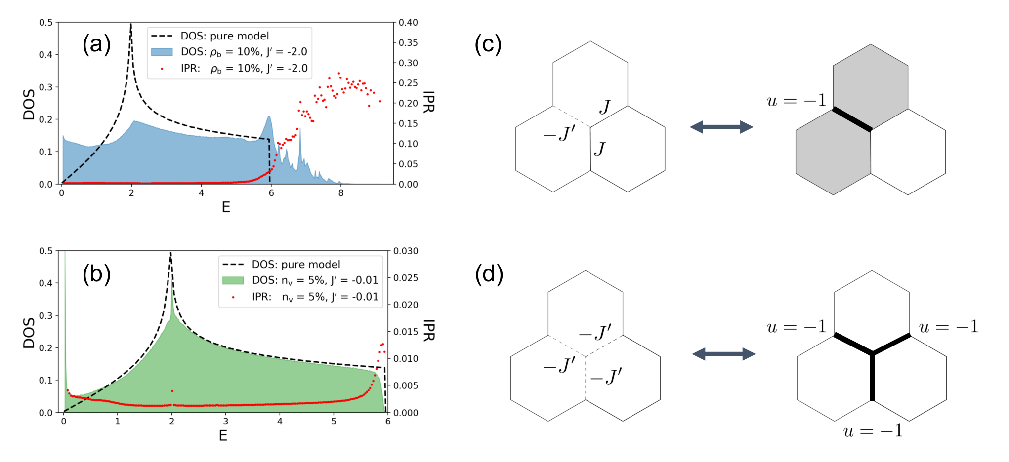
Throughout this work, we consider the ferromagnetic interaction for both normal couplings () and random couplings (). In the Kitaev honeycomb model, the overall sign will not change the physics because it corresponds to a simple gauge transformation of the Majorana hopping Hamiltonian. However, if we keep the normal couplings ferromagnetic but turn the random couplings into antiferromagnetic, the spectrum and density of states may change drastically. In this appendix, we briefly summarize the effect of antiferromagnetic random couplings on the exactly-solvable Kitaev honeycomb model.
Here we consider two scenarios of turning random into antiferromagnetic couplings: random bonds with and , corresponding to Fig. 2 (e), and the case of quasivacancies with and , corresponding to Fig. 2 (c). The calculation details are the same as in Fig. 2, with the only difference that becomes negative value on all the random couplings. In Fig. 10 (a)-(b), The numerical results show that in the former case of doped random bonds, the DOS is changed drastically by the transformation into negative , while in the latter case of quasivacncies, the DOS remains the same.
The difference between these two cases can be understood easily by the following argument. In the nearest-neighbor Majorana hopping Hamiltonian, the coupling strength and the link variable always appear as a product, namely, each hopping term in the Hamiltonian is in the form of , such that the transformation from ferro- to antiferromagnetic interaction is equivalent to the local flip of variable:
| (19) |
Therefore, these local flips may or may not change the flux sector of the system, depending on the real-space distribution of random bonds . In Fig. 10 (c)-(d), we demonstrate that the sign change of has an equivalent effect to the local flip of u variables.
In the case of random bonds, transformation from to is equivalent as keeping ferromagnetic but flipping on the same bond, leading to the creation of a flux pair. As a result, at finite density of random couplings, the flux sector will become similar to the random-flux sector as in Fig. 2 (j)-(l), and the flux configuration is determined by the real-space distribution of the antiferromagnetic bonds.
On the other hand, in the case of quasivacancy, random couplings always appear as trimers, such that the flux sector remains intact before and after the transformation. This explains why the sign change of has no effect on the density of states. In summary, we show that the random antiferromagnetic couplings can lead to different behaviors for the bond-disordered and site-diluted Kitaev spin liquid based on the local geometry of the random bonds, providing an interesting future perspective for the disorder effect in Kitaev materials.
References
- Anderson (1973) P. W. Anderson, Mater. Res. Bull. 8, 153 (1973).
- Huse and Elser (1988) D. A. Huse and V. Elser, Phys. Rev. Lett. 60, 2531 (1988).
- Laughlin (1983) R. B. Laughlin, Phys. Rev. Lett. 50, 1395 (1983).
- Kalmeyer and Laughlin (1987) V. Kalmeyer and R. B. Laughlin, Phys. Rev. Lett. 59, 2095 (1987).
- Lee (2008) P. A. Lee, Science 321, 1306 (2008).
- Balents (2010) L. Balents, Nature 464, 199 (2010).
- Savary and Balents (2017a) L. Savary and L. Balents, Rep. Prog. Phys. 80, 016502 (2017a).
- Zhou et al. (2017) Y. Zhou, K. Kanoda, and T.-K. Ng, Rev. Mod. Phys. 89, 025003 (2017).
- Knolle and Moessner (2019) J. Knolle and R. Moessner, Annu. Rev. Condens. Matter Phys. 10, 451 (2019).
- Broholm et al. (2020) C. Broholm, R. J. Cava, S. A. Kivelson, D. G. Nocera, M. R. Norman, and T. Senthil, Science 367 (2020).
- Takagi et al. (2019) H. Takagi, T. Takayama, G. Jackeli, G. Khaliullin, and S. E. Nagler, Nat. Rev. Phys. 1, 264 (2019).
- Kitaev (2006) A. Kitaev, Annals of Physics 321, 2 (2006).
- Norman (2016) M. R. Norman, Rev. Mod. Phys. 88, 041002 (2016).
- Shimizu et al. (2003) Y. Shimizu, K. Miyagawa, K. Kanoda, M. Maesato, and G. Saito, Phys. Rev. Lett. 91, 107001 (2003).
- Itou et al. (2008) T. Itou, A. Oyamada, S. Maegawa, M. Tamura, and R. Kato, Phys. Rev. B 77, 104413 (2008).
- Powell and McKenzie (2011) B. J. Powell and R. H. McKenzie, Rep. Prog. Phys. 74, 056501 (2011).
- Isono et al. (2014) T. Isono, H. Kamo, A. Ueda, K. Takahashi, M. Kimata, H. Tajima, S. Tsuchiya, T. Terashima, S. Uji, and H. Mori, Phys. Rev. Lett. 112, 177201 (2014).
- Yamashita et al. (2017) S. Yamashita, Y. Nakazawa, A. Ueda, and H. Mori, Phys. Rev. B 95, 184425 (2017).
- Okamoto et al. (2007) Y. Okamoto, M. Nohara, H. Aruga-Katori, and H. Takagi, Phys. Rev. Lett. 99, 137207 (2007).
- Jackeli and Khaliullin (2009) G. Jackeli and G. Khaliullin, Phys. Rev. Lett. 102, 017205 (2009).
- Chaloupka et al. (2010) J. Chaloupka, G. Jackeli, and G. Khaliullin, Phys. Rev. Lett. 105, 027204 (2010).
- Singh and Gegenwart (2010) Y. Singh and P. Gegenwart, Phys. Rev. B 82, 064412 (2010).
- Singh et al. (2012) Y. Singh, S. Manni, J. Reuther, T. Berlijn, R. Thomale, W. Ku, S. Trebst, and P. Gegenwart, Phys. Rev. Lett. 108, 127203 (2012).
- Plumb et al. (2014) K. W. Plumb, J. P. Clancy, L. J. Sandilands, V. V. Shankar, Y. F. Hu, K. S. Burch, H.-Y. Kee, and Y.-J. Kim, Phys. Rev. B 90, 041112 (2014).
- Sears et al. (2015) J. A. Sears, M. Songvilay, K. W. Plumb, J. P. Clancy, Y. Qiu, Y. Zhao, D. Parshall, and Y.-J. Kim, Phys. Rev. B 91, 144420 (2015).
- Rau et al. (2016) J. G. Rau, E. K.-H. Lee, and H.-Y. Kee, Annu. Rev. Condens. Matter Phys. 7, 195 (2016).
- Trebst (2017) S. Trebst, arXiv:1701.07056 (2017).
- Kitagawa et al. (2018) K. Kitagawa, T. Takayama, Y. Matsumoto, A. Kato, R. Takano, Y. Kishimoto, S. Bette, R. Dinnebier, G. Jackeli, and H. Takagi, Nature 554, 341 (2018).
- Motome and Nasu (2020) Y. Motome and J. Nasu, J. Phys. Soc. Jpn. 89, 012002 (2020).
- Knolle et al. (2015) J. Knolle, D. L. Kovrizhin, J. T. Chalker, and R. Moessner, Phys. Rev. B 92, 115127 (2015).
- Knolle et al. (2014a) J. Knolle, D. L. Kovrizhin, J. T. Chalker, and R. Moessner, Phys. Rev. Lett. 112, 207203 (2014a).
- Banerjee et al. (2016) A. Banerjee, C. A. Bridges, J.-Q. Yan, A. A. Aczel, L. Li, M. B. Stone, G. E. Granroth, M. D. Lumsden, Y. Yiu, J. Knolle, S. Bhattacharjee, D. L. Kovrizhin, R. Moessner, D. A. Tennant, M. D. G., and S. E. Nagler, Nat. Mater. (2016).
- Banerjee et al. (2017) A. Banerjee, J. Yan, J. Knolle, C. A. Bridges, M. B. Stone, M. D. Lumsden, D. G. Mandrus, D. A. Tennant, R. Moessner, and S. E. Nagler, Science 356, 1055 (2017).
- Ko et al. (2010) W.-H. Ko, Z.-X. Liu, T.-K. Ng, and P. A. Lee, Phys. Rev. B 81, 024414 (2010).
- Sandilands et al. (2015) L. J. Sandilands, Y. Tian, K. W. Plumb, Y.-J. Kim, and K. S. Burch, Phys. Rev. Lett. 114, 147201 (2015).
- Knolle et al. (2014b) J. Knolle, G.-W. Chern, D. L. Kovrizhin, R. Moessner, and N. B. Perkins, Phys. Rev. Lett. 113, 187201 (2014b).
- Nasu et al. (2016) J. Nasu, J. Knolle, D. L. Kovrizhin, Y. Motome, and R. Moessner, Nat. Phys. 12, 912 (2016).
- Rousochatzakis et al. (2019) I. Rousochatzakis, S. Kourtis, J. Knolle, R. Moessner, and N. B. Perkins, Phys. Rev. B 100, 045117 (2019).
- Sahasrabudhe et al. (2020) A. Sahasrabudhe, D. A. S. Kaib, S. Reschke, R. German, T. C. Koethe, J. Buhot, D. Kamenskyi, C. Hickey, P. Becker, V. Tsurkan, A. Loidl, S. H. Do, K. Y. Choi, M. Grüninger, S. M. Winter, Z. Wang, R. Valentí, and P. H. M. van Loosdrecht, Phys. Rev. B 101, 140410 (2020).
- Wang et al. (2020) Y. Wang, G. B. Osterhoudt, Y. Tian, P. Lampen-Kelley, A. Banerjee, T. Goldstein, J. Yan, J. Knolle, H. Ji, R. J. Cava, J. Nasu, Y. Motome, S. E. Nagler, D. Mandrus, and K. S. Burch, npj Quantum Mater. 5, 14 (2020).
- Wulferding et al. (2020) D. Wulferding, Y. Choi, S.-H. Do, C. H. Lee, P. Lemmens, C. Faugeras, and K.-Y. Gallais, Yann andChoi, Nat. Commun. 11, 1603 (2020).
- Halász et al. (2016) G. B. Halász, N. B. Perkins, and J. van den Brink, Phys. Rev. Lett. 117, 127203 (2016).
- Halász et al. (2017) G. B. Halász, B. Perreault, and N. B. Perkins, Phys. Rev. Lett. 119, 097202 (2017).
- Halász et al. (2019) G. B. Halász, S. Kourtis, J. Knolle, and N. B. Perkins, Phys. Rev. B 99, 184417 (2019).
- Katsura et al. (2010) H. Katsura, N. Nagaosa, and P. A. Lee, Phys. Rev. Lett. 104, 066403 (2010).
- Nasu et al. (2014) J. Nasu, M. Udagawa, and Y. Motome, Phys. Rev. Lett. 113, 197205 (2014).
- Nasu et al. (2015) J. Nasu, M. Udagawa, and Y. Motome, Phys. Rev. B 92, 115122 (2015).
- Hirobe et al. (2017) D. Hirobe, M. Sato, Y. Shiomi, H. Tanaka, and E. Saitoh, Phys. Rev. B 95, 241112 (2017).
- Kasahara et al. (2018a) Y. Kasahara, K. Sugii, T. Ohnishi, M. Shimozawa, M. Yamashita, N. Kurita, H. Tanaka, J. Nasu, Y. Motome, T. Shibauchi, and Y. Matsuda, Phys. Rev. Lett. 120, 217205 (2018a).
- Kasahara et al. (2018b) Y. Kasahara, T. Ohnishi, Y. Mizukami, O. Tanaka, S. Ma, K. Sugii, N. Kurita, H. Tanaka, J. Nasu, Y. Motome, et al., Nature 559, 227 (2018b).
- Nasu et al. (2017) J. Nasu, J. Yoshitake, and Y. Motome, Phys. Rev. Lett. 119, 127204 (2017).
- Metavitsiadis et al. (2017) A. Metavitsiadis, A. Pidatella, and W. Brenig, Phys. Rev. B 96, 205121 (2017).
- Pidatella et al. (2019) A. Pidatella, A. Metavitsiadis, and W. Brenig, Phys. Rev. B 99, 075141 (2019).
- Nasu and Motome (2020) J. Nasu and Y. Motome, Phys. Rev. B 102, 054437 (2020).
- Widmann et al. (2019) S. Widmann, V. Tsurkan, D. A. Prishchenko, V. G. Mazurenko, A. A. Tsirlin, and A. Loidl, Phys. Rev. B 99, 094415 (2019).
- Li and Chen (2020) M. Li and G. Chen, MRS Bulletin 45, 348 (2020).
- Feng et al. (2020) K. Feng, N. B. Perkins, and F. J. Burnell, Phys. Rev. B 102, 224402 (2020).
- Willans et al. (2010) A. J. Willans, J. T. Chalker, and R. Moessner, Phys. Rev. Lett. 104, 237203 (2010).
- Willans et al. (2011) A. J. Willans, J. T. Chalker, and R. Moessner, Phys. Rev. B 84, 115146 (2011).
- Watanabe et al. (2014) K. Watanabe, H. Kawamura, H. Nakano, and T. Sakai, J. Phys. Soc. Jpn. 83, 034714 (2014).
- Halász et al. (2014) G. B. Halász, J. T. Chalker, and R. Moessner, Phys. Rev. B 90, 035145 (2014).
- Zschocke and Vojta (2015) F. Zschocke and M. Vojta, Phys. Rev. B 92, 014403 (2015).
- Sreejith et al. (2016) G. J. Sreejith, S. Bhattacharjee, and R. Moessner, Phys. Rev. B 93, 064433 (2016).
- Savary and Balents (2017b) L. Savary and L. Balents, Phys. Rev. Lett. 118, 087203 (2017b).
- Yamaguchi et al. (2017) H. Yamaguchi, M. Okada, Y. Kono, S. Kittaka, T. Sakakibara, T. Okabe, Y. Iwasaki, and Y. Hosokoshi, Sci. Rep. 7, 16144 (2017).
- Kimchi et al. (2018) I. Kimchi, J. P. Sheckelton, T. M. McQueen, and P. A. Lee, Nat. Commun. 9, 4367 (2018).
- Slagle et al. (2018) K. Slagle, W. Choi, L. E. Chern, and Y. B. Kim, Phys. Rev. B 97, 115159 (2018).
- Li et al. (2018) Y. Li, S. M. Winter, and R. Valentí, Phys. Rev. Lett. 121, 247202 (2018).
- Knolle et al. (2019) J. Knolle, R. Moessner, and N. B. Perkins, Phys. Rev. Lett. 122, 047202 (2019).
- Takahashi et al. (2019) S. K. Takahashi, J. Wang, A. Arsenault, T. Imai, M. Abramchuk, F. Tafti, and P. M. Singer, Phys. Rev. X 9, 031047 (2019).
- Do et al. (2020) S.-H. Do, C. H. Lee, T. Kihara, Y. S. Choi, S. Yoon, K. Kim, H. Cheong, W.-T. Chen, F. Chou, H. Nojiri, and K.-Y. Choi, Phys. Rev. Lett. 124, 047204 (2020).
- Murayama et al. (2020) H. Murayama, Y. Sato, T. Taniguchi, R. Kurihara, X. Z. Xing, W. Huang, S. Kasahara, Y. Kasahara, I. Kimchi, M. Yoshida, Y. Iwasa, Y. Mizukami, T. Shibauchi, M. Konczykowski, and Y. Matsuda, Phys. Rev. Research 2, 013099 (2020).
- Yamada (2020) M. G. Yamada, npj Quantum Mater. 5, 82 (2020).
- Kao et al. (2021) W.-H. Kao, J. Knolle, G. B. Halász, R. Moessner, and N. B. Perkins, Phys. Rev. X 11, 011034 (2021).
- Hermanns et al. (2018) M. Hermanns, I. Kimchi, and J. Knolle, Annu. Rev. Condens. Matter Phys. 9, 17 (2018).
- Majumder et al. (2015) M. Majumder, M. Schmidt, H. Rosner, A. A. Tsirlin, H. Yasuoka, and M. Baenitz, Phys. Rev. B 91, 180401 (2015).
- Johnson et al. (2015) R. D. Johnson, S. C. Williams, A. A. Haghighirad, J. Singleton, V. Zapf, P. Manuel, I. I. Mazin, Y. Li, H. O. Jeschke, R. Valentí, and R. Coldea, Phys. Rev. B 92, 235119 (2015).
- Bahrami et al. (2019) F. Bahrami, W. Lafargue-Dit-Hauret, O. I. Lebedev, R. Movshovich, H.-Y. Yang, D. Broido, X. Rocquefelte, and F. Tafti, Phys. Rev. Lett. 123, 237203 (2019).
- Anderson (1958) P. W. Anderson, Phys. Rev. 109, 1492 (1958).
- Mott (1967) N. Mott, Adv. Phys. 16, 49 (1967).
- Abrahams et al. (1979) E. Abrahams, P. W. Anderson, D. C. Licciardello, and T. V. Ramakrishnan, Phys. Rev. Lett. 42, 673 (1979).
- Lee and Ramakrishnan (1985) P. A. Lee and T. V. Ramakrishnan, Rev. Mod. Phys. 57, 287 (1985).
- Shklovskii and Efros (1984) B. I. Shklovskii and A. L. Efros, Electronic Properties of Doped Semiconductors (Springer, 1984).
- Kramer and MacKinnon (1993) B. Kramer and A. MacKinnon, Rep. Prog. Phys. 56, 1469 (1993).
- Abrahams (2010) E. Abrahams, 50 Years of Anderson Localization (World Scientific Publishing Co, 2010).
- Evers and Mirlin (2008) F. Evers and A. D. Mirlin, Rev. Mod. Phys. 80, 1355 (2008).
- Baskaran et al. (2007) G. Baskaran, S. Mandal, and R. Shankar, Phys. Rev. Lett. 98, 247201 (2007).
- Pereira et al. (2008) V. M. Pereira, J. M. B. Lopes dos Santos, and A. H. Castro Neto, Phys. Rev. B 77, 115109 (2008).
- Lifshitz (1965) I. M. Lifshitz, Soviet Physics Uspekhi 7, 549 (1965).
- Feng et al. (2021) K. Feng, M. Ye, and N. B. Perkins, arXiv:2103.14661 (2021).
- Zotos et al. (1997) X. Zotos, F. Naef, and P. Prelovsek, Phys. Rev. B 55, 11029 (1997).
- Hentrich et al. (2020) R. Hentrich, X. Hong, M. Gillig, F. Caglieris, M. Čulo, M. Shahrokhvand, U. Zeitler, M. Roslova, A. Isaeva, T. Doert, L. Janssen, M. Vojta, B. Büchner, and C. Hess, Phys. Rev. B 102, 235155 (2020).
- Baek et al. (2020) S.-H. Baek, H. W. Yeo, S.-H. Do, K.-Y. Choi, L. Janssen, M. Vojta, and B. Büchner, Phys. Rev. B 102, 094407 (2020).