Robust Estimation of Tree Structured Models

Let $X=(X_{1},\ldots,X_{d})$ be a random vector with values in a finite product space $\mathcal{X}=\prod_{i=1}^{d}\mathcal{X}_{i}$. Without loss of generality we assume $\mathcal{X}_{i}=\{0,\ldots,r_{i}-1\}$, $r_{i}\in\mathbb{N}$, $r_{i}\geq 2$. Let $T^{*}$ be a tree with vertices $V=\{1,\ldots,d\}$, representing the components of the random vector $X=(X_{1},\ldots,X_{d})$, and with edges $E^{*}$. The distribution $p$ of $X$ is Markov with respect to $T^{*}$ if

where $\phi_{ij}:\mathcal{X}_{i}\times\mathcal{X}_{j}\to(0,+\infty)$ are some functions, called potentials. By the Hammersley-Clifford theorem we get then conditional independence characterization in terms of separation in the tree, that is, $X_{i}\mbox{\,$\perp\!\!\!\perp$\,}X_{j}|X_{C}$ if $C\subset V$ separates $i$ and $j$ in $T^{*}$; c.f. Theorem 3.9 in [14]. In the binary case, when $\mathcal{X}_{i}=\{0,1\}$, we equivalently write

where $h_{i},\beta_{ij}\in\mathbb{R}$ and $Z(h,\beta)$ is the normalizing constant. The corresponding model is called the Ising model on $T^{*}$.

The set of distributions that are Markov with respect to $T^{*}$ can be equivalently described by the following Markov process on the tree $T^{*}$. Fix any inner node $\rho\in V$, call it the root, and direct all edges of $T^{*}$ away from $\rho$. Denote by $p_{\rho}$ the marginal distribution of $X_{\rho}$ and, for each edge $u\to v$, let $M^{uv}$ be the matrix representing the conditional distribution $p_{v|u}$ of $X_{v}$ given $X_{u}$; $M_{x_{u},x_{v}}^{uv}=p_{v|u}(x_{v}|x_{u})$ for $x_{u}\in\mathcal{X}_{u}$, $x_{v}\in\mathcal{X}_{v}$. Then

Thus, fixing a directed version of $T^{*}$ fixes a parameterization of the set of all distributions Markov to $T^{*}$ making it into a parametric statistical model.

Suppose that $X\in\mathcal{X}$ has distribution $p$ that is Markov with respect to $T^{*}$. Given a random sample from $p$, the goal is to recover the underlying tree. As we mentioned in the Introduction, this problem can be solved very efficiently both from the computational and statistical point of view by the Chow-Liu algorithm [7], which outputs the tree that maximizes the likelihood function. Maximizing other functionals like AIC or BIC is also possible [9]. As we see next, the problem of structure recovery becomes more complicated in presence of corrupted data, which is the focus of this paper.

Assume now that the vector $X$ is not observed directly. Instead, we observe $X^{e}=(X_{1}^{e},\ldots,X_{d}^{e})$, a corrupted version of $X$. Here the only crucial assumption is that for every $i\in V$ the distribution of $X_{i}^{e}$ depends on $X$ only through the value of $X_{i}$.

The simplest corruption model is a direct generalization of the one used for the Ising models in [13]: $X_{i}$ gets corrupted with some probability $q_{i}$ and, if that happens, the corrupted value takes uniformly any of the remaining values. In other words, for every $i=1,\ldots,d$ and $k,l\in\mathcal{X}_{i}$

It is sensible to assume that $q_{i}$ is relatively small but our main results do not rely on this assumption. In fact, we consider a much more general corruption model given, for each $i\in V$, by any square stochastic matrix $M^{i}=[p_{kl}^{i}]$ with

Our problem can be therefore formulated as follows. Given the distribution of the corrupted version $X^{e}$ of $X$ recover (i) the underlying tree $T^{*}$, and (ii) the underlying distribution of $X$. As we argue in the next section, this problem can be naturally formulated in the language of latent tree models. The resulting links with phylogenetics provide new insights and a rich resource of relevant results that establish conditions under which $T^{*}$ can be recovered from the noisy data.

Given a tree $T=(W,E)$ with nodes $W$ and edges $E$, the underlying tree model for the random vector $Y$ with values in the discrete space $\mathcal{Y}=\prod_{i\in W}\mathcal{Y}_{i}$ is the set of all distributions over $\mathcal{Y}$ that are Markov with respect to $T$ as defined in Section 2.1. Suppose now that

is the set of vertices of $T$ corresponding to the leaves of $T$ (vertices of degree one). The set of marginal distributions of $X:=Y_{L}$ is called the latent tree model over $T$ and denoted $M_{\mathcal{Y}}(T)$. For a more detailed discussion see Section 1.1 in [22].

In general, the theory of latent tree models can be quite complicated; see [20]. In this paper we restrict to the most tractable case where the cardinality of each $\mathcal{Y}_{i}$ is the same, $|\mathcal{Y}_{i}|=r$ for every $i\in W$. In this case the corresponding latent tree model is often called the general Markov model and we denote it by $M_{r}(T)$.

Our problem of recovering $T^{*}$ and the underlying distribution from the noisy observations $X^{e}$ is very closely connected to the classical problem of recovering $T$ in a latent tree model $M_{r}(T)$. Before we explain this connection in Section 3.4, we first recall the corresponding classical results following [5].

A natural subset of square matrices that is reconstructible from rows is obtained by restricting the diagonal entries to dominate the other entries in the corresponding column. We also formulate the following assumptions on a latent tree model $M_{r}(T)$:

1. (A0)

   $T$ has no nodes of degree two.

2. (A1)

   The root distribution satisfies $p_{\rho}(x_{\rho})>0$ for all $x_{\rho}\in\{0,\ldots,r-1\}$.

3. (A2)

   For each edge $u\to v$ the transition matrix $M^{uv}=[p_{v|u}(x_{v}|x_{u})]$ is invertible and it is not a permutation matrix.

4. (A3)

   For each edge $u\to v$ the transition matrix $M^{uv}$ is reconstructible from rows.

The following result follows immediately from Proposition 3.1 and Theorem 4.1 in [5].

Identifiability results developed in phylogenetics, like the one above, play a crucial role in this paper. In our situation however it is important to consider the case where the condition (A0) does not hold. Then, the tree can never be recovered uniquely. For a simple illustration consider two models, one of a single edge $\bullet\!-\!\bullet$ and one on the chain $\bullet\!-\!\circ\!-\!\bullet$, where the middle vertex represents a latent variable. In case all three variables involved have $r$ states, the family of distributions over the solid nodes in both models is the same.

Denote by $\overline{T}$ the tree obtained from $T$ by suppressing all the degree two nodes. The following result can be found, for example, in Section 5.3.4 in [21].

The tree structure recovery in Theorem 3.2 can be in fact done using only pairwise marginal distributions and this fact has important consequences for the rest of the paper. For any edge $u\to v$ denote by $P^{uv}$ the $r\times r$ matrix of the marginal distribution of $(X_{u},X_{v})$, and by $P^{uu}$ a diagonal matrix with the marginal distribution of $X_{u}$ on the diagonal. For any two vertices $u,v$ let

where the denominator is non-zero if all marginal distributions are strictly positive. By essentially the same argument as in [19, Theorem 8.4.3] we obtain the following path-product formula

where $\overline{ij}$ denotes the unique path between $i$ and $j$ in $T$.

It can be shown (c.f. Section 2.2 in [22]) that

Because both $M^{uv}$ and $M^{vu}$ are stochastic matrices, all their eigenvalues lie in the unit circle. In particular, $\tau_{uv}\in[-1,1]$ and it is equal to $\pm 1$ precisely when $M^{uv}$ is a permutation matrix, or in other words, if $X_{u}$ and $X_{v}$ are functionally related. With assumptions (A1) and (A2) we have thus that $\tau_{uv}^{2}\in(0,1)$. Define

then (3) implies that

In other words $d_{uv}$ represent lengths of edges in the tree $T$ and $d_{ij}$ are then distances between vertices calculated by summing the lengths of edges on the unique path between them in $T$. The collection of distances between the leaves $D=[d_{ij}]_{i,j\in L}$ is called a tree metric.

The following classical result assures that $T$ can be recovered from the underlying tree metric; see Theorem 1 in [4].

As we mentioned above the assumptions of this theorem are automatically satisfied for $d_{ij}=-\log\tau_{ij}$ in the general Markov model as long as the assumptions (A0), (A1), and (A2) hold. We finish this section giving the explicit link between latent tree models and tree models for corrupted data.

As in Section 2, consider a tree $T^{*}$ representing a random vector $X=(X_{1},\dots,X_{d})$ and assume that each $X_{i}$ can take $r$ states (from now on $r_{i}=r$ for $i=1,\dots,d$). We assume that the distribution of $X$ is Markov with respect to $T^{*}$, so in particular we can fix a root at an inner node $\rho$ and consider transition matrices at the directed edges.

We let $T^{e}$ be the tree obtained from $T^{*}$ by adding $d$ extra vertices representing the noisy variables $X_{i}^{e}$ and by linking each $X_{i}$ with $X_{i}^{e}$ by an edge with the corresponding transition matrix $M^{i}$; see Figure 1 for an example. Then $T^{e}$ is a rooted tree with the root $\rho$. Note that $X_{i}^{e}$ is independent of $\{X_{j},X_{j}^{e}:\;j\neq i\}$ given $X_{i}$ and so the vector $(X,X^{e})$ is Markov with respect to the augmented tree $T^{e}$. Consequently, the distribution of $X^{e}$ lies in the latent tree model $M(T^{e})$.

To recover $T^{*}$ from the distribution of $X^{e}$ we first try to recover $T^{e}$. For that, note that $T^{e}$ has a special topology with each inner vertex having one and only one leaf-child. The degree two nodes in $T^{e}$ correspond precisely to the leaves of $T^{*}$. This special topology of $T^{e}$ plays a crucial role in the rest of this paper.

In our case, the tree $\overline{T^{e}}$ is obtained by suppressing in $T^{e}$ the nodes that correspond to the leaves of $T^{*}$; c.f. Definition 3.4. For the tree in Figure 1, the tree $\overline{T^{e}}$ is given on the left in Figure 2.

Recall that in this new language, the goal is to recover $T^{*}$ from a distribution $p\in M_{r}(T^{e})$.

Denote by $[T^{*}]$ the set of all trees $S$ over the vertex set $V=\{1,\ldots,d\}$ such that $\overline{S^{e}}=\overline{T^{e}}$. Here we mean equality as semi-labelled trees, that is, $\overline{S^{e}}$ and $\overline{T^{e}}$ must have the same topology and labelling of the leaf nodes but the labelling of the inner nodes is irrelevant. Directly by construction, $T^{*}\in[T^{*}]$. For another example, let $T^{*}$ be the tree on the left in Figure 1, where the corresponding tree $T^{e}$ is given on the right. The tree $\overline{T^{e}}$ is given on the left in Figure 2. Now let $S$ be a tree like $T^{*}$ but 3 swapped with 1 and 2 swapped with 4. The corresponding tree $S^{e}$ is depicted on the right in Figure 2 and $\overline{S^{e}}=\overline{T^{e}}$.

By Proposition 3.5, if $S\in[T^{*}]$ then

and so we cannot distinguish from the corrupted data between the trees in $[T^{*}]$ because each $S\in[T^{*}]$ leads to the same model $M_{r}(\overline{T^{e}})$ for $X^{e}$. Theorem 4.1 implies the following result.

The tree $\overline{T^{e}}$ is one natural way of representing the equivalence class $[T^{*}]$. To have a concrete description of this equivalence class directly in terms of $T^{*}$ call an inner node of $T^{*}$ a mother if it is adjacent to at least one leaf of $T^{*}$. For example, the root and the node 2 in the tree $T^{*}$ in Figure 1 are mothers.

As a byproduct of Theorem 4.2 and this characterization of the class of $[T^{*}]$ we obtain:

We next discuss two somewhat extreme examples that show that $[T^{*}]$ can be large or small depending on $T^{*}$.

This shows that the equivalence class $[T^{*}]$ can be still potentially quite large. We now discuss extra assumptions that allow us to identify $T^{*}$ uniquely.

It is possible to completely identify the tree $T^{*}$ under a mild assumption on the noise of the mother nodes. We formulate this condition in terms of the distances $d_{ij}=-\log\tau_{ij}^{2}$ defined in Section 3.3.

In terms of the parameters of the distribution, condition (A4) translates to

where $M^{uv}$ denotes the conditional distribution of the variable represented by the node $v$ given the variable represented by the node $u$. In particular, for the Ising model on $T^{*}$, this is equivalent to saying that

for each mother $u$ and each of its adjacent leaves $i$. In other words, the correlation between $X_{u}$ and its noisy version is greater than the correlation between $X_{u}$ and the noisy version of any other variable; hardly a controversial assumption to make.

Recall that the Chow-Liu algorithm [7] relies on computing mutual informations and building the maximum cost spanning tree of the resulting weighted graph. Following the debate in [13] on whether the Chow-Liu method is a good method to recover the tree structure for noisy data, we study the conditions under which noisy data still allow for consistent estimation of the correct tree in some specific cases. We focus on the situation when for every $i,j$ the mutual information $I(X_{i},X_{j})$ between $X_{i}$ and $X_{j}$ is a strictly decreasing function of the distance $d_{ij}=-\log\tau_{ij}^{2}$. This includes the binary Ising model with no external field and more generally the fully symmetric tree models on $r$ states; see Lemma 6 in [6]. The fully symmetric model on $r$ states is a tree model such that each variable has $r$ states and uniform marginal distribution. Moreover, each transition matrix is of the form

In the special case when the mutual informations $I(X_{i},X_{j})$ are strictly decreasing function the distances $d_{ij}=-\log\tau^{2}_{ij}$, we can equivalently build the minimum cost spanning tree based on the distances $D=[d_{ij}]$. For consistency argument, we can replace the sample correlations $\hat{\rho}_{ij}$ with the actual correlations of the data generating distribution. In this case $D=[d_{ij}]$ forms a tree metric on $T^{*}$ and $T^{*}$ is the (unique) minimum cost spanning tree of the complete graph weighted with $D$; we write $T^{*}={\rm MWST}(D)$. This implies that the Chow-Liu algorithm is a consistent tree recovery method.

To consider consistency of the Chow-Liu algorithm for noisy data note that now the corresponding distances are $\bar{d}_{ij}=-\log\bar{\tau}_{ij}^{2}$ where $\bar{\tau}_{ij}$ are defined for $(X_{i}^{e},X_{j}^{e})$. We have

and so $\overline{D}=[\bar{d}_{ij}]$ does not form a tree metric on $T^{*}$. In the next theorem we provide conditions on the noise distribution that assure that the Chow-Liu method remains a consistent method for the unique recovery of the true underlying tree $T^{*}$. In other words, we study the conditions under which $T^{*}={\rm MWST}(\overline{D})$. We will use the notation $\ell_{i}:=d_{ii^{e}}=-\log(\tau_{ii^{e}}^{2})$.

Note that the condition $d_{uv}>\ell_{u}-\ell_{v}$ is equivalent to $d_{uv^{e}}>d_{uu^{e}}$, which is a natural assumption in many applications. In case this condition does not hold, Theorem 4.8 assures that $T^{*}$ can be still uniquely identified as long as the condition $d_{uv}>\ell_{u}-\ell_{v}$ holds for all cases when $u$ is a mother node and $v$ is one of its leaves. It is just that this identifiability cannot be in general obtained using the Chow-Liu algorithm.

There is a handful of algorithms that can be used to learn $\overline{T^{e}}$ (or equivalently $[T^{*}]$); see, for example, [6, 15]. In case unique recovery conditions in Theorem 4.8 hold, we can recover $T^{*}$ from $\overline{T^{e}}$ by shrinking for each inner node the shortest of its terminal edges.

One of the most widely used methods to recover a phylogenetic tree from evolutionary pairwise distances is Neighbor-Joining (briefly NJ) [17]. In order to test the performance of this method in the recovery of $\overline{T^{e}}$ or $T^{*}$ from noisy data, we have simulated corrupted data on each of the trees $T^{*}$ of Figure 3. We have restricted ourselves to the fully symmetric model on $r$ states for $r=2$ and $r=4$ (also known as the Jukes-Cantor model, [11]) both for the stochastic matrices $M^{uv}$ and $M^{i}$. For each edge $u\rightarrow v$ of $T^{*}$, we have set the off-diagonal entries of $M^{uv}$ equal to $0.20$ for $r=2$ and to $0.07$ for $r=4$ so that the distance $d_{u,v}$ equals 1 for $r=2$ and $2$ for $r=4$. In order to see how the performance of the method varies when the noise increases, we have set all distances $d_{i,i^{e}}$ equal to $\ell$ and let $\ell$ vary from $0.01$ up to $3$ for $r=2$ and up to $4$ for $r=4$ in intervals of $0.1$. Note that in practice we do not expect $\ell$ to be larger than $1$ ($X_{i}$ should be correlated more with its noisy version than with other variables). Finally, for each set of parameters we considered $1000$ experiments, each with sample size $5000$ from the corresponding tree distribution.

Using the normalized Robinson-Foulds distance (as implemented in [18]), we measure how far is the recovered tree from the original tree class $[T^{*}]$ (that is, from $\overline{T^{e}}$). Note that NJ always outputs binary trees while the trees $\overline{T^{e}}$ we are considering are not binary trees. Thus, we set a tolerance $\varepsilon$ such that if the estimated length of an internal edge is smaller than $\varepsilon$, we shrink that edge. In Figure 4 we show the results for different values of $\varepsilon$. We observe that the best results are obtained when $\varepsilon$ is about half of the length of the branches of $T^{*}$. As expected, as the noise $\ell$ (the length of the corrupted branches) increases, it becomes more difficult to recover $\overline{T^{e}}$. For example,when $\ell$ is smaller than the length of the original edges of the tree (i.e. $\ell\leq 1$ for $r=2$ or $\ell\leq 2$ for $r=4$), then we obtain highly successful results for almost all values of $\varepsilon$. It is worth noting that for $\ell=2$ we have transition matrices with condition number $2.72$ for $r=2$ and $1.4$ for $r=4$; similarly, for $\ell=3$ transition matrices have condition number $4.48$ for $r=2$ and $1.65$ for $r=4$. This has to be taken into account in relation to the hypothesis $(A2)$ about the invertibility of transition matrices (see Theorem 4.1) and gives an insight to the different performance we obtain for $r=2$ and $r=4$.

In practice, the choice of the threshold $\varepsilon$ from data could be done in a data-driven manner. However, any such procedure would be better implemented if there were some previous knowledge on the noise level or on underlying tree. Indeed, the case of a chain tree is dramatically different than a star tree with the former being the one that gives best results and the star tree the worst.

For the binary tree, we have also implemented a slightly different procedure for tree recovery that uses the prior knowledge that the underlying tree is binary: we shrink the shortest internal edges of the tree output by NJ until the internal structure (i.e. removing external edges) gives a binary tree. We present these results in Figure 5. In this case, we obtain excellent results for $r=4$ (in both cases, for $r=2$ and $r=4$, the results are similar to the ones obtained with $\varepsilon=0.5$ and $1$, respectively).

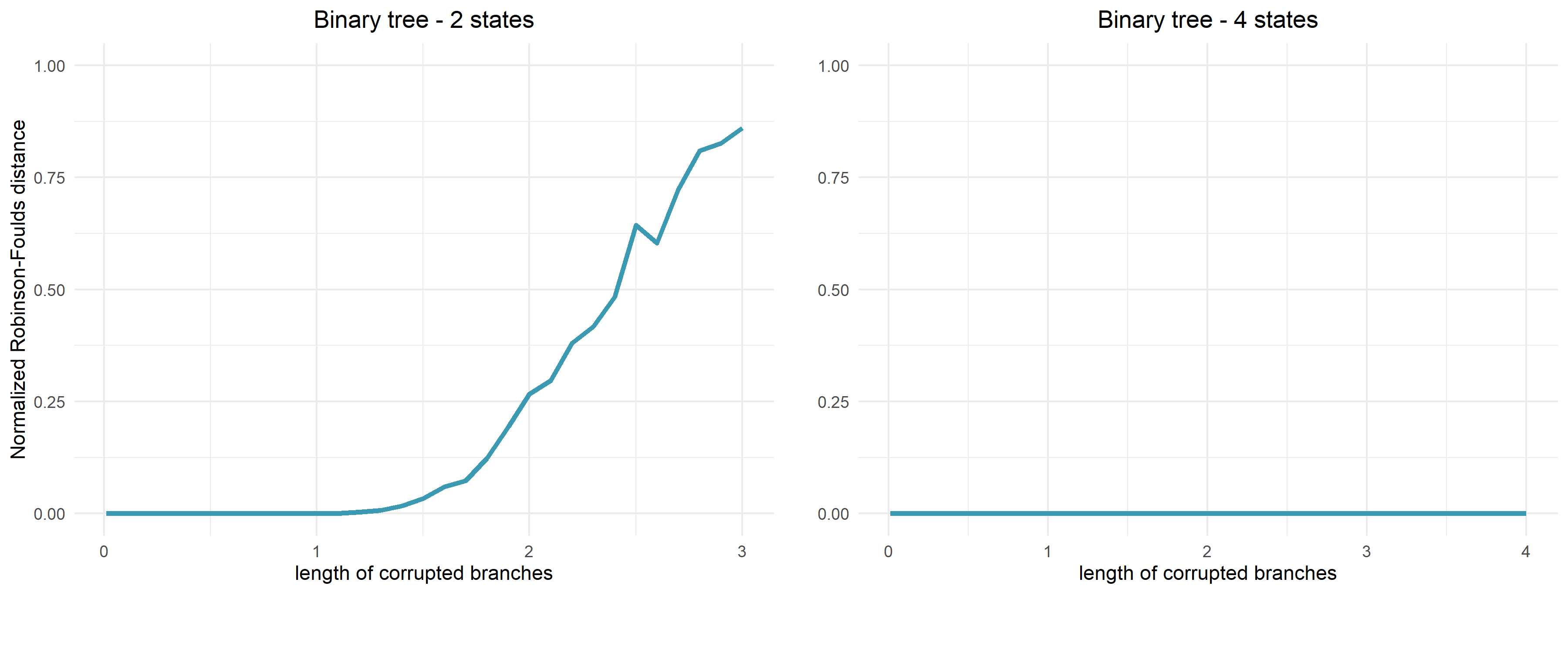
We also implemented the recovery of $T^{*}$ based on Theorem 4.8 for the same simulated data. If $\overline{T^{e}}$ is correctly obtained, then $T^{*}$ is successfully reconstructed most of the times (so we do not include figures with this information) for all the trees. Actually, for the binary and the star tree, $T^{*}$ is correctly recovered 100% of the times (both for $r=2$ and $r=4$, and for any $\varepsilon$). For the chain tree the performance drops slightly for $r=2$ and $\ell>0.5$. In this case 94% of the times when $T^{*}$ is not correctly identified, the recovered tree differs from $T^{*}$ by one leaf.

In this section the vector $X$ takes values in any product space $\mathcal{X}=\prod_{i=1}^{d}\mathcal{X}_{i}$, where $\mathcal{X}_{i}$ do not have to be discrete. We consider that $X$ follows a linear model on the tree $T^{*}$. This means that $X$ is Markov with respect to $T^{*}$ and for every edge $u\to v$ on the rooted version of $T^{*}$ the conditional expectation $\mathbb{E}(X_{v}|X_{u})$ is an affine function of $X_{u}$. Models of this type were first discussed in [1]. A canonical example of such a situation is the Gaussian model on $T^{*}$. However, it also includes the discrete case discussed earlier. We explain this last connection in the following example.

The fact that Gaussian undirected tree models fall into this category follows because the undirected graphical model over $T^{*}$ can be represented by a system of linear equations on the rooted version of $T^{*}$, where for each edge $u\to v$ we have $X_{v}=\lambda_{uv}X_{u}+\epsilon_{v}$ with $\lambda_{uv}\in\mathbb{R}$ and $\epsilon_{v}$ being zero-mean Gaussian and independent of each other. Then $\mathbb{E}[X_{v}|X_{u}]=\lambda_{uv}X_{u}$ is linear.

In general, let each variable $X_{u}$ for $u\in V$ be modelled as a random vector in $\mathbb{R}^{r-1}$ for a fixed $r$. Each variable can be either discrete or continuous but we add a requirement that:

1. (AL1)

   The matrix $\Sigma_{vv}=\mathbb{E}X_{v}X_{v}^{T}-\mathbb{E}X_{v}(\mathbb{E}X_{v})^{T}$ is positive definite for every $v\in V$.
   

This assumption has an analogous role as assumption (A1) for general Markov models.

To complete the model description we also assume that the corrupted version $X^{e}$ of $X$ depends in a linear way on $X$ in the sense that $\mathbb{E}(X_{u}^{e}|X_{u})$ is an affine function of $X_{u}$ for every $u\in V$. As always, we assume that $X_{i}^{e}$ depends on $X$ only through the value of $X_{i}$. If $X$ follows a linear model on the tree $T^{*}$ then $(X,X^{e})$ follows a linear model on the corresponding tree $T^{e}$. Our goal is to show that in this case we can recover the equivalence class $[T^{*}]$ from the distribution of $X^{e}$.

The distribution of $X^{e}$ gives a tree metric on $T^{e}$. Define the normalized version $\bar{X}_{v}$ of $X_{v}$ as

Denoting $\Sigma_{uv}=\mathbb{E}X_{u}X_{v}^{T}-\mathbb{E}X_{u}(\mathbb{E}X_{v})^{T}$ we obtain

where we used that $\mathbb{E}[X_{u}|X_{v}]$ is affine, or equivalently, that $\mathbb{E}[X_{u}|X_{v}]=\mathbb{E}X_{u}+\Sigma_{uv}\Sigma_{vv}^{-1}(X_{v}-\mathbb{E}X_{v})$. In analogy to (A2) we assume:

References

- [1] Animashree Anandkumar, Kamalika Chaudhuri, Daniel J Hsu, Sham M Kakade, Le Song, and Tong Zhang. Spectral methods for learning multivariate latent tree structure. In Advances in Neural Information Processing Systems, pages 2025–2033, 2011.
- [2] Vijay Badrinarayanan, Ignas Budvytis, and Roberto Cipolla. Semi-supervised video segmentation using tree structured graphical models. IEEE transactions on pattern analysis and machine intelligence, 35(11):2751–2764, 2013.
- [3] Guy Bresler, Mina Karzand, et al. Learning a tree-structured Ising model in order to make predictions. Annals of Statistics, 48(2):713–737, 2020.
- [4] Peter Buneman. The recovery of trees from measures of dissimilarity. Mathematics in the archaeological and historical sciences, 1971.
- [5] Joseph T Chang. Full reconstruction of Markov models on evolutionary trees: identifiability and consistency. Mathematical biosciences, 137(1):51–73, 1996.
- [6] Myung Jin Choi, Vincent YF Tan, Animashree Anandkumar, and Alan S Willsky. Learning latent tree graphical models. Journal of Machine Learning Research, 12:1771–1812, 2011.
- [7] CK Chow and CN Liu. Approximating discrete probability distributions with dependence trees. Information Theory, IEEE Transactions on, 14(3):462–467, 1968.
- [8] Ciro D’Elia, Giovanni Poggi, and Giuseppe Scarpa. A tree-structured markov random field model for bayesian image segmentation. IEEE Transactions on Image processing, 12(10):1259–1273, 2003.
- [9] David Edwards, Gabriel CG De Abreu, and Rodrigo Labouriau. Selecting high-dimensional mixed graphical models using minimal AIC or BIC forests. BMC Bioinformatics, 11(1):18, 2010.
- [10] WN Everitt. A note on positive definite matrices. Glasgow Mathematical Journal, 3(4):173–175, 1958.
- [11] TH Jukes and CR Cantor. Evolution of protein molecules. In Mammalian Protein Metabolism, pages 21–132, 1969.
- [12] Ashish Katiyar, Jessica Hoffmann, and Constantine Caramanis. Robust estimation of tree structured Gaussian graphical model. arXiv preprint arXiv:1901.08770, 2019.
- [13] Ashish Katiyar, Vatsal Shah, and Constantine Caramanis. Robust estimation of tree structured Ising models. arXiv preprint arXiv:2006.05601, 2020.
- [14] S. L. Lauritzen. Graphical Models. Clarendon Press, Oxford, United Kingdom, 1996.
- [15] Elchanan Mossel, Sébastien Roch, and Allan Sly. Robust estimation of latent tree graphical models: Inferring hidden states with inexact parameters. IEEE transactions on information theory, 59(7):4357–4373, 2013.
- [16] Konstantinos E Nikolakakis, Dionysios S Kalogerias, and Anand D Sarwate. Predictive learning on hidden tree-structured Ising models. arXiv preprint arXiv:1812.04700, 2018.
- [17] N. Saitou and M. Nei. The neighbor-joining method: a new method for reconstructing phylogenetic trees. Molecular Biology and Evolution, 4(4):406–425, 1987.
- [18] K.P. Schliep. Phangorn: Phylogenetic analysis in R. Bioinformatics, 27(4):592–593, 2011.
- [19] Charles Semple and Mike Steel. Phylogenetics, volume 24. Oxford University Press, 2003.
- [20] Nevin L Zhang. Hierarchical latent class models for cluster analysis. The Journal of Machine Learning Research, 5:697–723, 2004.
- [21] Piotr Zwiernik. Semialgebraic Statistics and Latent Tree Models. Number 146 in Monographs on Statistics and Applied Probability. Chapman & Hall, September 2015.
- [22] Piotr Zwiernik. Latent tree models. In Handbook of Graphical Models, pages 283–306. CRC Press, 2018.