Range Estimation of a Moving Target Using Ultrasound Differential Zadoff-Chu Codes
Abstract
High accuracy range estimation is an essential tool required in many modern applications and technologies. However, continuous range estimation of a moving target is a challenging task, especially under Doppler effects. This paper presents a novel signal design, which we name differential Zadoff-Chu (DZC). Under Doppler effects, DZC sequences improve the performance of the maximum likelihood (ML)-based range estimation compared to its performance when using regular ZC sequences. Moreover, a reduced-complexity ranging algorithm is proposed utilizing DZC sequences and is shown to outperform the regular ZC ML-based range estimation. The proposed system is evaluated in a typical indoor environment, using a low-cost ultrasound hardware. Under a low signal to noise ratio ( dB SNR), more than of the range estimates are in less than mm error, with a movement range from m to m and a maximum velocity of m/s. For the same movement range, the system provides range estimates with a root mean square error (RMSE) less than mm in a high SNR scenario ( dB), and a MSE less than mm in a low SNR scenario ( dB). For a larger movement range from m to m with a maximum velocity of m/s, the proposed system provides range estimates with RMSE less than mm at dB SNR.
Index Terms:
Differential coding, Differential Zadoff-Chu Sequences, Doppler estimation, Maximum-Likelihood estimation, ultrasound, movement estimation.I Introduction
Many modern applications require estimating the range between two devices with very high accuracy. These applications include navigation, medical care, location-aware networks, video gaming, and virtual reality, to name a few. Consequently, range estimation has been studied, using different approaches, based on ultrasound, radio, infrared or laser signals [1, 2, 3, 4].
Although algorithms based on infrared or lasers have high accuracy, they are complicated and expensive [5]. Likewise, radio-signal-based range estimation approaches utilizing the received signal strength (RSS) of a Wi-Fi or a Bluetooth signal require pre-calibration and provide low accuracy [6]. While radio-based ranging methods, through time of flight (TOF) estimation, do not require pre-calibration [7], they still need an accurate synchronization. In fact, owing to the high speed of light, small timing errors result in large ranging errors. Therefore, approaches based on ultra-wideband radio signals have typically a 10-20 cm accuracy [8]. In contrast, ultrasound-based methods are of low cost and have high accuracy in estimating the signal TOF, thanks to the low propagation speed of ultrasound signals [9]. Indeed, one of the widely used commercial UWB positioning systems is Pozyx [10] which claims up to 10 cm positioning accuracy. On the other hand, the commercially available ultrasound-based positioning system, Marvel Mind [11], claims a positioning accuracy of 2 cm. Consequently, this paper considers ultrasound-based ranging.
Despite the type of the utilized technology, ranging waveforms can be categorized into two general classes: continuous wave (CW) and pulsed. Despite that CW ranging is more susceptible to multipaths and echos, still it has many advantages over pulsed ranging. The main advantage of the CW ranging is that it maximizes the total transmitted power, because the transmitter is continuously transmitting. Moreover, the CW ranging can provide a much higher update rate, i.e. number of range estimates per second, as compared to pulsed ranging. Therefore, in this paper we are focusing on continuous range estimation [12].
In addition to the aforementioned ranging technologies, various range estimation methods have been proposed in the literature. Although RSS-based ranging algorithms are generally simple compared to other algorithms, they suffer from low accuracy [13]. Conversely, phase-shift-based ranging using a single frequency signal has high accuracy. However, its application is limited to distances less than one wavelength of the signal carrier [14]. Using multiple frequencies allows the estimation of longer distances by calculating phase differences between the various frequencies. The authors in [15] use a narrowband multi-frequency continuous wave (MFCW) ultrasound signal for range estimation. Nevertheless, the difference between the multiple frequencies, , in the MFCW restricts the estimated range to where is the speed of sound. Furthermore, range estimation based on narrowband signals is very sensitive to noise, multipath, and interference. As a result, a number of range estimation systems utilizing wideband signals have been proposed to diminish the limitations of narrowband signals in TOF estimation.
In basic TOF-based ranging systems, the peak location of the cross-correlation between the transmitted and the received signals provides an estimate of the TOF, assuming that the transmitter and the receiver are synchronized. Indeed, perfect synchronization can be achieved by sharing the same clock between the transmitter and the receiver. After that, multiplying the TOF by the propagation speed of the signal determines the range between the transmitter and the receiver. Hence, the correlation properties of the transmitted signal highly affect the accuracy of the estimated TOF. Due to their good correlation properties, Zadoff-Chu sequences are widely used for synchronization purposes. In our previous work [16], a high accuracy TOF-based ranging system has been implemented utilizing a Zadoff-Chu-coded ultrasound signal. However, with a moving transmitter or receiver, Doppler shifts were found to severely degrade the range estimation accuracy, especially for high-speed moving devices and/or long transmitted signal.
Range estimation of a moving target can be achieved by transmiting sine waves at multiple frequencies, followed by a frequency modulated continuous waves (FMCW) [17]. The authors in [17], use the Fast Fourier transform (FFT) of the sine waves and the FMCW to determine the velocity and range of the moving target, respectively. The downside of this approach is the assumption of a constant velocity over the duration of the transmitted signal, which limits its application to targets with low acceleration.
Under a low-acceleration assumption, joint maximum likelihood (ML) estimation of the target’s velocity and range achieves very high accuracy [18]. However, the ML approach requires a two-dimensional search which has high computational complexity [19], as will be shown in this paper. Furthermore, if the target has a high acceleration, an additional search dimension is required to consider the acceleration of the target.
Another low-complexity solution to remove Doppler is to differentially encode the transmitted signal. Applying differential decoding at the receiver side removes Doppler. In [20], the authors propose differential polyphase codes to resolve the frequency ambiguity. Another implementation of differential encoding/ decoding is demonstrated in [21]. In this paper, we propose a new signal design based on the idea of differential encoding.
The main contributions of the paper are as follows.
- •
We propose a novel signal design, which we name Differential Zadoff-Chu, and we study its properties.
- •
We derive the maximum likelihood (ML) estimator and use it to estimate the TOF and Doppler shift.
- •
We propose a low-complexity ranging algorithm, utilizing Differential Zadoff-Chu sequences, and show that, under Doppler, it outperforms the benchmark ranging algorithms, namely the regular Zadoff-Chu ML-based, the FMCW short-time Fourier transform (STFT)-based [17], multiple signal classification (MUSIC)-based line spectral estimation (LSE) [22] and super-resolution radar, via minimization program [23].
- •
We experimentally evaluate the proposed ranging system in a typical indoor environment using low-cost ultrasound hardware.
II Problem Formulation
Zadoff-Chu (ZC) sequences are polyphase complex valued sequences, named after Solomon A. Zadoff and D.C. Chu [24],[25]. These sequences have the constant amplitude and zero auto-correlation (CAZAC) property, which allows them to provide high accuracy TOF-based range estimation of a static target, using cross-correlation [16]. However, random Doppler shifts tend to break the CAZAC property of the ZC sequences, especially for long sequences and/or high-velocity moving targets as will be shown in this section.
Under Doppler, a wide-band signal encounters time scaling (compression and/ or expansion) proportional to the relative speed between the transmitter and the receiver. Therefore, the passband received ultrasound signal can be modeled as [26]
| (1) |
where is the passband transmitted signal, is the attenuation incurred by propagation, is the relative Doppler shift defined as the ratio of the relative velocity to the speed of sound , is the TOF, is the overall phase shift encountered by the carrier and is an additive Gaussian noise, with zero mean and variance .
The time scaling of the received signal is due to the fact that Doppler translates each frequency component by a different amount [26]. We propose two ranging algorithms in this paper, one is based on maximum likelihood (ML) estimation and the other is a low-complexity ranging algorithm. In the ML-based ranging, we use the baseband version of the wideband received signal model given by Equation (1). Whereas in the low-complexity ranging algorithm, we approximate the received signal model using the narrowband time-delayed and Doppler shifted signal model [27]. To compensate for the error due to the narrowband approximation, we apply a phase shift refinement algorithm using the wideband model (1). Therefore , the narrowband approximation of the received signal can be written as
where is the Doppler shift at time . The complex envelope, , of the received signal can be obtained using an IQ demodulator. Moreover, the discrete-time version of the complex envelope of the received signal, obtained by sampling , at sampling period , is given by
| (2) | ||||
where is the channel response at discrete-time under Doppler, is the discrete-time complex envelope of the transmitted signal, is the TOF normalized by and rounded to the nearest integer, is the discrete-time normalized Doppler shift and is a discrete-time complex additive Gaussian noise with zero mean and variance . In addition, the transmitted signal is composed of repetitions of a sequence of length , where we assume that the symbols of the sequence are transmitted according to the sampling rate . Therefore, the transmitted signal is periodic and this periodicity condition is required in our ranging algorithms as will be illustrated in section IV. If the target displacement over the sequence duration is less than several meters, then the change in the attenuation factor over the sequence duration is negligible [28]. This assumption is met in the case of this paper. Therefore, it can be assumed that for .
Let the complex envelope of the transmitted signal be a ZC sequence of length which is given by
| (3) |
where is given by
| (4) |
and , is coprime with . It can be shown that in the noiseless case, and under a fixed (i.e. constant over the duration of the ZC sequence) Doppler shift , the magnitude of the cross-correlation between the complex envelope of the transmitted and received signal is given by [16]
| (5) |
This implies that the magnitude of the cross-correlation function has a peak whenever both the numerator and denominator are zeros, which depends on both the TOF and the Doppler shift . Therefore, the location of this peak does not give the true TOF except when is zero. Actually, when is not zero, the location of the cross-correlation peak is shifted proportionally to the value of . As a result, the out of phase value of the magnitude of the cross-correlation is nonzero, i.e. the Doppler shift breaks the CAZAC property of the ZC sequences.
III Differential Zadoff-Chu Sequence and Its Properties
To mitigate Doppler shifts and improve range estimation accuracy, we propose a new code , called Differential ZC (DZC), given by
| (6) |
where
| (7) |
and , , is coprime with . The proposed sequences are named Differential Zadoff-Chu sequences because they are derived based on differential sliding correlation defined in section (III-A). As we show in Appendix B, Differential ZC sequences are periodic, with period if is odd and not divisible by 3, if is odd and divisible by 3, if is even and either or is divisible by 3, and otherwise.
We claim that under the assumption of a high symbol rate, i.e. number of symbols per second, DZC sequences almost preserve the CAZAC property even in the presence of random Doppler shifts. Moreover, we claim that for any sequence length, , using coherent detection, DZC sequences provide better range estimation accuracy compared to the regular ZC sequences.
To prove the first claim, we utilize a differential sliding correlation approach and show that, under a high symbol rate, DZC sequences almost preserve the CAZAC property, even if there are random Doppler shifts. To prove the second claim, we evaluate the mean square error (MSE) for estimating the range and velocity of a moving target for regular and differential ZC sequences, both by simulation and real experiments.
III-A Robustness to Doppler
In this subsection, we will show that DZC codes maintain the CAZAC property even under random Doppler shifts by using a differential sliding correlation, defined as
| (8) |
for , where is the differential correlation step. DZC sequences are designed such that for any differential correlation step , the product is a regular ZC sequence. Therefore, we end up correlating the differentially received samples with a regular ZC sequence. Here we are applying circular differential sliding correlation where . The complex envelope of the received signal is cut into frames each of length . The differentially decoded frame at instant is obtained by multiplying the frame at instant with the conjugate of the frame that starts at .
Now, consider an odd-length DZC. In the noiseless case and with , using (II) and (7) we can rewrite the equation above as
Under a high symbol rate with respect to Doppler spread, it can be assumed that , since for practical Doppler shifts, the channel will not change too much between two consecutive samples and hence . As an example, in our setup the symbol duration is around msec. Therefore, even with an acceleration of m/, the change in velocity over one symbol duration will be mm/s. This velocity change will shift a kHz signal by around Hz which is negligible. Consequently, choosing removes the highest amount of Doppler residual.
Considering the noiseless case to simplify the analysis, the differential sliding correlation becomes
| (9) | ||||
| (10) | ||||
| (11) |
Taking the absolute value finally yields the desired result
| (12) |
Similarly, we can show that an even-length DZC sequence has a differential sliding correlation also given by (12). This shows that the out of phase value of the magnitude of the differential sliding correlation is zero, hence the proposed DZC sequence maintains the CAZAC property, even under random Doppler shifts. Lastly, we would like to highlight that applying the differential sliding correlation to ZC sequences, with odd or even length , will give a constant magnitude for all lags, i.e. . Therefore, applying differential correlation to ZC sequences does not provide a way to estimate the range of the target.
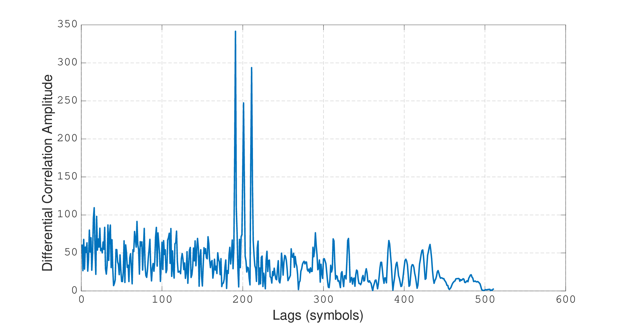
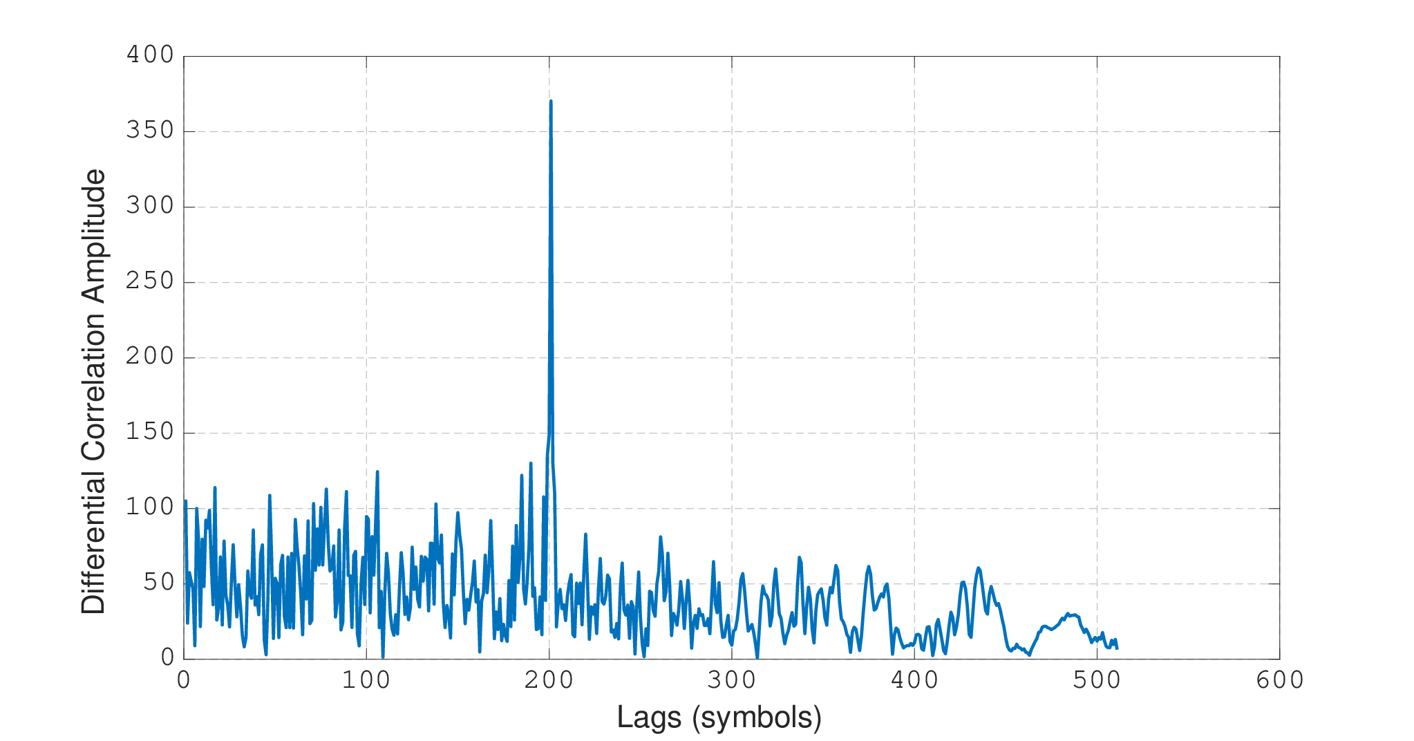
Finally, we would like to illustrate the ability of the proposed DZC codes and differential correlation to estimate the ranges to multiple targets. To do so, each target transmits a unique DZC code of the same length (a DZC code with the same but different value of ). We address three situations where we have three transmitters placed at three different distances. Therefore, the received signal coming from each transmitter is delayed by a different TOF (, and ). In the first situation, the three transmitters transmit the same DZC code. In Figure 1 (a), the received signal is composed of three similar DZC codes () and we notice that the differential correlation gives three peaks located at the respective TOFs. This means that the three transmitted signals are very correlated, as expected, since they have the same DZC code. In the second situation, each transmitter transmits a DZC code with the same but different value of . Figure 1 (b) shows the correlation between a DZC code with and the received signal which is composed of three different DZC codes (, , and ). Due to the orthogonality between the codes, the correlation vector has a single peak located at the TOF of the DZC code with . In the last situation, one transmitter transmits a DZC code and the other two transmitters transmit a ZC code. Figure 1 (c) shows the correlation vector between a DZC code with the received signal which is composed of a DZC code with and two ZC codes with and . Again, due to orthogonality, the correlation vector has a single peak located at the TOF of the first DZC code. Therefore, there is orthogonality between different DZC codes and between a DZC code and a ZC code. Consequently, by assigning each user a unique DZC code, we can perform multi-target range estimation.

IV Range Estimation Algorithms
We will derive the maximum likelihood (ML) estimator, for both ZC and DZC sequences, in section A, which gives us a benchmark. We will then derive a low-complexity algorithm based on DZC in section B. While it has inferior performance to the ML applied on the DZC, it still outperforms the ML estimator applied on the ZC. Moreover, the low complexity ranging algorithm accurately estimates the range even under random Doppler shifts, while the ML-based ranging requires a fixed Doppler shift over the duration of the transmitted sequence.
Finally, we will propose a refinement algorithm, based on phase shift estimation, to compensate for the loss with respect to the performance of the ML estimator.
IV-A Maximum Likelihood Estimator
Under a fixed Doppler shift over the duration of the transmitted sequence, the complex envelope of the received signal can be written as
| (13) |
where is the carrier frequency offset, is the carrier frequency of the transmitted signal and is the velocity of the target over the duration of the transmitted signal. The probability of the received sequence, whether regular or differential ZC, is given by
| (14) |
The phase changes too much from one measurement to the other and generally a precise priori knowledge about it cannot be obtained or even processed easily. The best way is to assume the worst case scenario of a totally unknown phase with a uniform distribution over . Averaging over will enable us to focus on and , on which conditioning remains after averaging. Therefore, the PDF in (14) becomes
| (15) |
By expanding the term inside the summation in Equation (15), the likelihood function can be written as
| (16) |
where
| (17) | ||||
| (18) | ||||
| (19) |
Alternatively, we can write (16) as
| (20) | ||||
| (21) | ||||
| (22) |
where (21) follows from the fact that the added angle has no effect on the integration of the cosine over its period. Here, is the modified Bessel function of the first kind and zero order. The modified Bessel function can be approximated as [29]
| (23) |
Therefore, under a high SNR scenario, the likelihood function can be approximated as
| (24) |
Maximizing the likelihood function is equivalent to maximizing the log-likelihood function which, up to a constant, is given by
| (25) |
where we replaced , , by their expressions. In the high SNR scenario, the last term in Equation (25) is negligible and the log-likelihood function reduces to
| (26) |
The first term can be ignored since the signal itself has a constant amplitude and does not affect the maximization. Therefore, maximizing the log-likelihood function can be achieved by maximizing the following metric
| (27) | ||||
| (28) |
where is obtained by re-sampling to the new sampling frequency , with .
The argument of the module in (28) is known in pulsed radar and sonar signal processing as the ambiguity function, because it might have several maxima which causes ambiguity in estimating and . To illustrate this ambiguity, consider a transmitted odd-length ZC sequence and let us focus on the noiseless case with a negligible time scaling, i.e. . Then, using (II) and (4), the metric (28) becomes
| (29) |
where and are the true TOF and true Doppler shift, respectively. The metric in (29) has a maximum whenever the quantity is an integer multiple of , which causes ambiguity in determining the TOF. Figure 2 (a) shows the ambiguity function which has several maxima. To avoid this ambiguity we limit our search over and to a window that includes a single maximum. Since the TOF hypothesis is in , the difference between the TOF hypothesis and the true TOF cannot exceed . For this reason we estimate the Doppler shift at time over a window centered at the previous Doppler shift estimate and has a width equal to , i.e. , where the search step is chosen small enough to detect the Doppler shift with high accuracy. For this estimation to be accurate, we need to know the initial Doppler shift . Also, the current true Doppler shift should not differ from the previous Doppler shift by more than . Assuming the target is static initially, makes the initial Doppler shift, , equals to zero. To guarantee that the difference between the current and the previous Doppler shift is less than , we utilize the periodicity of ZC codes as will be shown next.
Unlike regular ZC, using the proposed DZC sequences removes the ambiguity in estimating the TOF and Doppler shift. To illustrate this, consider an odd-length DZC sequence and let’s focus again on the noiseless case, then using Equations (II), and (7) the metric (28) becomes
| (30) |
This metric has maxima that occurs at and an integer. Therefore, the ambiguity is removed over and there will be no need for the assumption of known initial Doppler shift to unambiguously estimate the TOF. Figure 2 shows the ambiguity functions for the regular ZC and DZC sequence.


IV-B Reduced complexity ranging algorithm
The ML estimator has the lowest variance for all possible values of the estimation parameters, but it is computationally expensive. Therefore, we propose a reduced complexity range estimation algorithm that makes use of the CAZAC property by utilizing the proposed DZC sequences.
For repetitive and periodic transmission, the DZC sequence is repeated times. The received signal is processed using a sliding window with width to estimate the TOF and the Doppler shift. The step by which we move the window determines the update rate of the system, , which is the number of estimates per second. Setting gives the highest possible update rate. Figure 3 illustrates the processing of the received sequences, where the sliding window is applied with a step of one symbol.

Consider the window of the complex envelope of the received signal, applying differential sliding correlation gives
| (31) |
where is a circularly shifted version of the transmitted DZC sequence with a phase function , is the received sequence, and is the period of the sequence. The index , where is the index of the range estimate, and is the total number of range estimates . Therefore, with the circular shift differential sliding correlation, each DZC sequence of length gives us TOF estimates. As was shown in (8)-(11), taking the absolute value of the differential sliding correlation gives
| (32) |
Therefore, the location of the maximum of gives , which we call the initial TOF estimate. Multiplying the initial TOF estimate by the speed of sound gives the initial range estimate . The initial range estimates are accurate up to a sample resolution. If the true range is not an integer multiple of the sample resolution, then the fractional range will be rounded to the nearest sample. This rounding process causes errors in estimating the range. Therefore, in order to achieve sub-sample resolution and to improve the ranging immunity to noise, we estimate the phase shift between the transmitted and received DZC sequence and use it to refine the initial range estimates. However, in order to do that we need first to estimate and compensate for Doppler.
IV-B1 Doppler Estimation and Compensation
To estimate Doppler, we need to estimate the velocity over segments of the received sequence. The segment length, , which is a factor of the sequence length, , is chosen such that the change in velocity is negligible over the duration of the segment. The number of range estimates per segment is given by . Differentiating these range estimates gives instantaneous velocity estimates per segment. Averaging the velocity estimates and dividing by the speed of sound gives the relative Doppler shift of that segment.
The frequency offset, caused by the Doppler, translates into time scaling (compression or expansion) of the signal waveform [26], such that
| (33) |
where and are the transmitted and the received signal respectively. Inverse time scaling the received signal, using the estimated relative Doppler shift , compresses or expands the signal, and therefore removes the frequency offset. This is equivalent to re-sampling the bandpass signal by , leading to
| (34) |
The frequency offset estimation and compensation algorithm is implemented in two steps, as shown in Figure 4; first we estimate the relative Doppler shift, , using the initial range estimates. Then, we re-sample the segments of the received signal to the new sampling frequency . Figure 5 shows the transmitted and the received signals spectra before and after frequency offset compensation.


IV-B2 Phase Shift Estimation
After correcting the frequency offset of the received signal, we can refine the initial range estimates to a sub-sample resolution by estimating the phase shift between the transmitted and the corrected received signal.
Let the discrete-time version of the received signal after Doppler compensation be
| (35) |
where denotes the operation of rounding to the nearest integer. The circularly shifted version of the transmitted signal with a circular shift of is given by
| (36) |
The phase shift between and at the frequency bin is given by [30]
| (37) | ||||
| (38) |
where and are the discrete Fourier transforms of and respectively, denotes the complex conjugation operation, is the sub-sample delay, and is the error in the estimated phase due to noise. Dividing the estimated phase shift by the associated frequency bin and multiplying it by the speed of sound gives the estimated range refinement .
Since the DZC sequences have frequencies that vary with time, it is required to estimate the phase shift associated with each of these frequencies. Therefore, we determine the valid frequency bins of the received signal based on a particular threshold value. This value is decided experimentally to be 0.5 of the maximum of . All frequency bins that have components higher than this threshold are considered valid frequencies. The estimated range refinement is the average of for all valid frequency bins
| (39) |
where is the number of the valid frequency bins. Finally, the refined range is given by
| (40) |
IV-B3 Minimum Refinement Variance Search
Since the phase information is limited to , the range refinement is confined to one wavelength of the transmitted signal. Therefore, the phase shift algorithm fails when the absolute value of the error is larger than , where is the maximum wavelength of the signal, which might happen in low SNR scenarios. To correct the initial range estimates to within one wavelength, a minimum refinement variance search algorithm is applied. This algorithm calculates the variance in the estimated refinement over the valid frequency bins, at different range candidates.
Let be the circularly shifted version of where the index represents the amount by which we shift . Each circular shift of represents a range candidate, where the range candidate associated with zero cyclic shift is . Using instead of in (35)-(39) gives the estimated range refinement for each range candidate. The refinement variance associated with the range candidate is given by
| (41) |
When the absolute difference is less than , the estimated range refinements will be consistent over all the valid frequency bins which results in low variance . In contrast, when the difference is larger than , the estimated range refinements will fluctuate over the valid frequency bins which produces high variance . The proposed method estimates the refinement variance at different range candidates. The range candidate that has the minimum refinement variance over the valid frequency bins is chosen as the correct range estimate. Figure 6 shows refinement variance for a window of 200 range candidates before and after compensating for the frequency offsets under low SNR (-10 dB). The initial range estimate has an error of 6 samples,hence the location of the minimum variance is at -6. Therefore, the minimum variance search algorithm enables us to correct the initial range to within one wavelength of the signal.


Whether we use the full fledged ML receiver or its high SNR equivalent correlation, the proposed algorithm has a much lower complexity compared. While the performance of the proposed algorithm is slightly degraded compared to the DZC ML estimator, it still outperforms the ZC ML estimator.
V Experimental Setup
This section describes the experimental setup and the hardware used to test and evaluate the proposed system. We utilized IQ modulation to transmit the complex signals. In IQ modulation, the real part of the signal is modulated using a cosine wave and the imaginary part is modulated using a sine wave. The transmitter (Tx) used in this setup is a Pioneer TS-T110 tweeter which has a bandwidth of kHz with a central frequency of kHz Figure 7(a). The receiver (Rx) is a microphone on a Printed Circuit Board (PCB) Figure 7(b). XLR connectors link the transmitter and the receiver to the PC through a sound card (E44 Express) that provides a sampling rate up to kHz. The data is recorded as .wav files during experiments and saved in the PC to be processed off-line. The experiments are implemented in a typical indoor environment with dimensions cm X cm X cm. The speed of sound is assumed to be constant during the experiments ( m/s) due to the negligible changes in temperature and humidity.


An infrared tracking system (OptiTrack), which gives the ground truth with mm 3D accuracy and a maximum update rate of Hz [31], provides a benchmark for evaluating the performance of the proposed system . It uses a set of infrared cameras (up to sixteen cameras) to keep track of small spheres coated with retro-reflective film, thus providing accurate 3D location and orientation. Figure 8 shows the target that is tracked by the IR cameras with the transmitter attached to it. Figure 9 shows the experimental setup.


VI Results
VI-A Simulation Results
In this section, we compare different TOF estimation algorithms of a moving target using the same DZC sequence. All simulations were performed using MATLAB. The simulation results in this section were obtained from samples, unless stated otherwise. We compare the MSEs in estimating the TOF under a constant Doppler shift using MUSIC-based LSE algorithm [22] and the super-resolution radar, via solving minimization program [23] against the maximum likelihood estimator (MLE) and the proposed reduced-complexity algorithm. The MSEs in estimating the TOF under different SNR scenarios (with , symbols, , and ) are shown in Figure 10.

The MLE outperforms all the other algorithms at both low and high SNR scenarios. At a high SNR scenario, the proposed reduced-compelxity ranging algorithm outperforms both the MUSIC-based LSE algorithm [22] and the super-resolution radar estimation algorithm [23]. In addition, the proposed reduced-complexity algorithm requires much less computational cost compared to the MUSIC-based LSE and the super-resolution radar algorithms, as shown in Table (I). Because of the high computational complexity of the super-resolution radar algorithm and the MUSIC-based LSE, we chose in this comparison.
| Tx duration | MUSIC-based LSE [22] | Super-res radar [23] | Diff Corr |
| (ms) | (DZC) | (DZC) | (DZC) |
Next, we compare the performance of the differential sliding correlation-based ranging algorithm, using DZC sequences, against three other algorithms; short-time Fourier transform (STFT) on FMCW [17], the ML estimator using regular ZC sequences, and the ML estimator using DZC sequences, derived in section IV. For each of the four algorithms, a signal with a duration of 120 ms is generated. A moving target with a velocity of 1 m/s is simulated using MATLAB. The received signal is composed of the delayed, Doppler shifted transmitted signal with additive white Gaussian noise (AWGN) and a random phase shift. The mean square error (MSE) of the estimated TOF using the four algorithms are shown in Figure 11. In this simulation we are using a sampling frequency of kHz which makes each sample represents around 1.78 mm. Figure 11 shows that the MSE for the ML estimation using the DZC sequences is lower than the MSE for the regular ZC sequences, which means that ML estimation using DZC sequences can achieve higher accuracy compared to its accuracy when using regular ZC sequences.
Moreover, differential sliding correlation of the DZC sequences outperforms the ML estimation using regular ZC sequences under high SNR scenarios. Under low SNR scenarios, ML estimation has the best performance among the four algorithms. Furthermore, the differential sliding correlation ranging, using DZC sequences, outperforms the FMCW ranging algorithm [17]. Table (II) shows the running time for each of the four algorithms to estimate the range. From the table we can see that the differential sliding correlation has the lowest computational complexity among the four algorithms.

| Tx duration | Maximum Likelihood | STFT | Diff Corr |
| (ms) | (Diff or regular ZC) | (FMCW) | (Diff ZC) |
We run simulations to evaluate the performance of the proposed algorithm for different sequence lengths. Table III shows the root mean square error (RMSE) of the proposed algorithm for different sequence lengths under different SNR values and a fixed velocity of m/s. The results are obtained from observations. Short sequences, e.g. with and , have lower energy and therefore are less immune to noise as compared to longer sequences, and .
| SNR = 20 dB | 10 dB | 0 dB | -10 dB | |
| Length | RMSE | RMSE | RMSE | RMSE |
| (symbols) | (mm) | (mm) | (mm) | (mm) |
Then, we evaluate the performance of our algorithm under various velocities and for different bandwidths (from samples with fixed SNR dB). Table IV shows the RMSE for the differential correlation ranging algorithm using a 511-symbol DZC sequence, with different bandwidths and target velocities. As expected, the RMSE increases with velocity. Moreover, we notice that the RMSE increases with higher BW. The increase in the RMSE is due to the narrowband approximation of the received signal when using differential correlation as in Equation (II) (i.e. lower bandwidth means our approximation is more accurate).
| BW = 19.2 kHz | 6.4 kHz | 4.8 kHz | |
| Velocity | RMSE | RMSE | RMSE |
| (m/s) | (mm) | (mm) | (mm) |
Next, we evaluate the performance of different codes under various velocities with a fixed bandwidth of kHz and fixed SNR of dB. The proposed algorithm outperforms the benchmark algorithms under various velocities as can be seen in Figure 12.

VI-B Experimental Results
This section presents the experimental results as an evaluation of the proposed system. An ultrasound receiver on a printed circuit board (PCB) is fixed in a specific location, while an ultrasound transmitter is moving. A set of infrared cameras provides the location of the moving transmitter with sub-millimeter accuracy. The motion ground truth is found by converting the positions of both the transmitter and the receiver into ranges. A repetition of each of the four different signals was transmitted with a total duration of around 30 seconds, while the transmitter was stationary in the first few seconds, then moving forward and backward before stopping at a certain distance for the last few seconds.
The first experiment demonstrates the limitations of the regular ZC cross-correlation-based ranging, where a set of 511-symbol ZC sequence is used to track the moving transmitter. The estimated range is accurate when the transmitter is stationary. However, during the movement, the ranging accuracy significantly degrades due to Doppler. Figure 13 (a) shows the estimated range using the regular ZC sequence where the accuracy degradation due to Doppler is clear on the plot. The second experiment validates the ability of the proposed DZC to combat Doppler effect. In this experiment, a set of 511-symbol DZC sequence is utilized to track the moving transmitter with a similar velocity as in the first experiment. The speeds at the two experiments are very similar but not the same because we are dealing with human motion, which makes it not possible to maintain the exact same speed at all experiments, unlike when using robots. Figure 13 (b) illustrates the ability of the DZC sequence to track movements without being affected by Doppler. Figure 13 (c) shows the velocity of the moving target during the experiments. The results in Figures 13 are obtained using samples. Table V shows the mean square error (MSE) of the estimated range in those two experiments.


| Sequence Length | ZC Correlation-based | Reduced-complexity |
|---|---|---|
| (symbols) | MSE | MSE |
| () | () | |
The recorded data is processed under different SNR values, by adding white Gaussian noise to the data in the MATLAB, to validate the minimum refinement variance search algorithm. Figure 14 shows the percentage of range estimates that are correct up to half the wavelength of the maximum frequency (around 7.5 mm). As the SNR goes lower, the accuracy of the ranges estimated without using the minimum refinement variance search degrades, while the estimates obtained using the minimum variance search maintain high accuracy. Figures 15 (a), (b), (c), and (d) show the cumulative error with and without using the minimum refinement variance search algorithm under different SNR values. Using the minimum refinement variance search algorithm always improves the accuracy of the estimated range.


Table VI shows the MSE of the estimated ranges under different SNR values using differential correlation only, and using the reduced-complexity ranging algorithm. The reduced-complexity algorithm utilizes the differential correlation with the minimum refinement variance search and phase shift compensation, to reach sub-sample accuracy. The phase refinement improves the initial range estimates to very high accuracy even under low SNR scenario.
| SNR | diff-correlation only | Reduced-complexity Algorithm |
|---|---|---|
| (dB) | MSE | MSE |
| () | () | |
Figure 16 shows the MSE of the TOF estimation, using the three types of signals, under different SNR scenarios with a maximum velocity of m/s. The TOF estimation accuracy is dictated by the hardware bandwidth and sampling rate, which control the ranging resolution of the system. The ranging resolution of our experimental setup is around mm/sample. Therefore, any movement that is equivalent to a fraction of a sample is rounded to the nearest integer multiple of the sampling resolution. The phase refinement algorithm compensates for this fractional TOF, which improves the ranging accuracy compared to the other methods. Moreover, the minimum variance search shows the robustness of the reduced-complexity algorithm under low SNR scenarios compared to the other algorithms. Finally, we would like to highlight that the experimental performance of the DZC ML-based ranging accuracy can be improved if we make our grid search with a sub-sample resolution. However, this has a very high computational cost, hence is difficult to implement. We would like to highlight that the slight degradation in the performance of the proposed algorithm under low SNR scenario, as compared to the other algorithms, is due to the nature of the proposed differential decoding. By applying the differential decoding we double the noise, and therefore, under extremely low SNR values the accuracy degrades.

We evaluate the performance of the proposed algorithm using different sequence lengths under different SNR values. Table VII shows the RMSE for the proposed algorithm which is evaluated experimentally under different lengths. The results in Table VII are obtained from around samples and under different velocities with a maximum velocity of m/s. The velocity of the moving target is shown at Fig. 13 (c) . The experimental results show that with increasing sequence length, the algorithm becomes more robust to noise.
| SNR = 20 dB | 10 dB | 0 dB | -10 dB | |
| Length | RMSE | RMSE | RMSE | RMSE |
| (symbols) | (mm) | (mm) | (mm) | (mm) |
Finally, we evaluate the proposed code and algorithm against the benchmark algorithms for different velocities under fixed SNR value ( dB). At each experiment, the velocity of the moving target is varying with time. Table VIII shows the RMSE for the proposed and benchmark algorithms under different velocities. The proposed DZC sequences and ranging algorithms outperform the benchmark ranging algorithms. The degradation in the ZC-based ML ranging algorithm is due to the ambiguity in the joint estimation of the TOF and Doppler shift. Figure 17 shows the estimated range and velocity of a moving target, using the proposed ML-based DZC ranging algorithm, in two experiments. In Figure 17 (a) and (b) the maximum velocity of the moving target is m/s, and in Figure 17 (c) and (d) the maximum velocity is m/s . This figure shows that the proposed algorithm and signal design provides high ranging accuracy even under high velocities.
| ML ZC | CWLFM [17] | Diff DZC | ML DZC | |
| Max Velocity | RMSE | RMSE | RMSE | RMSE |
| (m/s) | (mm) | (mm) | (mm) | (mm) |


VII Conclusion
In this paper, a novel signal design based on the differential coding of ZC sequences is presented to estimate the range of a moving transmitter. The proposed DZC design and ranging algorithms were evaluated, both in simulation and using experimental setup in a typical indoor environment. The proposed DZC outperforms the regular ZC sequences in estimating the TOF and Doppler shift of a moving target, as shown using both simulations and real experiments. Moreover, the simulation results show that the proposed differential sliding correlation, using a DZC sequence, outperforms the benchmark algorithms, namely STFT-based range estimation, using a FMCW and ML range estimation, using a regular ZC sequence. The differential sliding correlation has the lowest computational complexity in estimating the range of a moving target compared to the benchmark algorithms.
The experimental results show that while the long typical ZC sequence fails to estimate the range of a moving transmitter using cross-correlation, the proposed DZC sequence is able to combat Doppler, by utilizing differential sliding correlation. The minimum refinement variance search algorithm is able to correct range estimates up to half the wavelength of the signal carriers even in low SNR scenarios, which provides robustness to the system. At low SNR (-12 dB), the minimum refinement variance search algorithm has 98% of the range estimates correct up to half wavelength of the signal carriers, compared to 92% when not using the algorithm.
The proposed low-complexity ranging algorithm, using a DZC sequence of 511 symbols, has a MSE of under SNR of dB, and a MSE of under SNR of dB, which shows the ability of the proposed system to achieve sub-sample resolution, even in low SNR scenarios. Moreover, the experimental results show that the low-complexity ranging and ML-based ranging algorithm, using DZC, outperforms the ML-based ZC ranging and the FMCW STFT-based ranging as expected.
Future Work
The proposed ranging system can be utilized in various applications that require estimating the position of a moving target. One such a system that requires high positioning accuracy is a robotic surgical system. Another widely used ranging-based application is indoor localization which requires estimating the distances between a receiver (known as the mobile device) and multiple transmitters (known as base-stations). These base-stations need to be synchronized. We can achieve synchronization by transmitting an RF signal with the ultrasound signal. After determining the distance between each base-station and the target, we can use a trilateration algorithm to find the position of the target. In indoor navigation applications, we can extend our current work to localize multiple users by giving each user a unique DZC code (i.e. a DZC code with a unique DZC exponent ). Each DZC code has a good auto-correlation property and poor cross-correlation with the other DZC codes which provides orthogonality between the various users. Moreover, the proposed ranging algorithm can be used in systems of low sampling rate where the ranging resolution is dictated by the sampling frequency, so the phase refinement can significantly improve the resolution of the system.
Appendix A Analytical Derivation of Differential Zadoff-Chu Sequence Design
The differential decoding of a Differential ZC sequence gives a ZC sequence which has a phase as a quadratic function of time. Therefor, the Differential ZC sequence has a phase as a cubic function of time
| (A.42) |
where . For an even length ZC sequence, (A.42) gives
, , , and is an arbitrary constant which is set to zero for simplicity. The phase of the differential ZC becomes
For an odd length ZC sequence, (A.42) gives
, , , and is an arbitrary constant which is set to zero for simplicity. The phase of the differential ZC becomes
Appendix B Periodicity of Differential Zadoff-Chu Codes
For repetitive and periodic transmission, each sequence is repeated times, where is an integer and each single sequence is referred to as a block. It is important to determine the period of the Differential ZC sequence to perform the periodic transmission.
For an even length Differential ZC sequence, with all the phases to be understood modulo , taking a shift of symbols in time gives
Therefore, shifting by results in the same sequence but with a phase change of up to an additive phase shift. If is even and either or is a multiple of 3, then the period of the sequence is . Otherwise, the period is .
Similarly considering an odd length Differential ZC sequence, with all the phases to be understood modulo gives
Therefore, shifting by results in the same sequence as but with a phase change of up to an additive constant phase shift. If is odd and not divisible by 3, then either or is even and divisible by 3, hence the sequence period is . Otherwise, if is odd and divisible by 3 then the sequence period is , which can be seen as follows
| (B.43) |
Since is odd, the term () is even, taking modulo gives
| (B.44) |
To sum up, the Differential ZC sequence is given by
| (B.45) |
where
| (B.46) |
and modulo , and modulo .
References
- [1] J. Hightower and G. Borriello, “A survey and taxonomy of location systems for ubiquitous computing,” IEEE computer, vol. 34, no. 8, pp. 57–66, 2001.
- [2] K. Whitehouse, C. Karlof, and D. Culler, “A practical evaluation of radio signal strength for ranging-based localization,” ACM SIGMOBILE Mobile Computing and Communications Review, vol. 11, no. 1, pp. 41–52, 2007.
- [3] Ç. Yüzbaşioğlu and B. Barshan, “Improved range estimation using simple infrared sensors without prior knowledge of surface characteristics,” Measurement Science and Technology, vol. 16, no. 7, p. 1395, 2005.
- [4] M.-C. Amann, T. Bosch, M. Lescure, R. Myllyla, and M. Rioux, “Laser ranging: a critical review of usual techniques for distance measurement,” Optical engineering, vol. 40, no. 1, pp. 10–19, 2001.
- [5] R. Rasshofer and K. Gresser, “Automotive radar and lidar systems for next generation driver assistance functions,” Advances in Radio Science, vol. 3, no. B. 4, pp. 205–209, 2005.
- [6] M. Cypriani, F. Lassabe, P. Canalda, and F. Spies, “Open wireless positioning system: A wi-fi-based indoor positioning system,” in Vehicular Technology Conference Fall (VTC 2009-Fall), IEEE 70th, 2009, pp. 1–5.
- [7] J.-Y. Lee and R. A. Scholtz, “Ranging in a dense multipath environment using an uwb radio link,” IEEE Journal on Selected Areas in Communications, vol. 20, no. 9, pp. 1677–1683, 2002.
- [8] R. M. Narayanan and M. Dawood, “Doppler estimation using a coherent ultrawide-band random noise radar,” IEEE Transactions on Antennas and Propagation, vol. 48, no. 6, pp. 868–878, 2000.
- [9] M. Kushwaha, K. Molnár, J. Sallai, P. Volgyesi, M. Maróti, and A. Lédeczi, “Sensor node localization using mobile acoustic beacons,” in IEEE International Conference on Mobile Adhoc and Sensor Systems Conference, 2005, pp. 9–17.
- [10] https://www.pozyx.io/. (2020) Pozyx system overview. [Online]. Available: https://www.pozyx.io/
- [11] https://marvelmind.com/. (2020) Marvel mind system overview. [Online]. Available: https://marvelmind.com/
- [12] M. I. Skolnik, “Introduction to radar systems,” New York, McGraw Hill Book Co., 1980. 590 p., 1980.
- [13] C. Medina, J. C. Segura, and S. Holm, “Feasibility of ultrasound positioning based on signal strength,” in 2012 International Conference on Indoor Positioning and Indoor Navigation (IPIN). IEEE, 2012, pp. 1–9.
- [14] F. Figueroa and E. Barbieri, “An ultrasonic ranging system for structural vibration measurements,” IEEE Transactions on Instrumentation and Measurement, vol. 40, no. 4, pp. 764–769, 1991.
- [15] C. Huang, M. Young, and Y. Li, “Multiple-frequency continuous wave ultrasonic system for accurate distance measurement,” Review of scientific instruments, vol. 70, no. 2, pp. 1452–1458, 1999.
- [16] M. H. AlSharif, M. Saad, M. Siala, T. Ballal, H. Boujemaa, and T. Y. Al-Naffouri, “Zadoff-chu coded ultrasonic signal for accurate range estimation,” in Signal Processing Conference (EUSIPCO), 2017 25th European. IEEE, 2017, pp. 1250–1254.
- [17] W. Mao, J. He, and L. Qiu, “Cat: high-precision acoustic motion tracking,” in Proceedings of the 22nd Annual International Conference on Mobile Computing and Networking. ACM, 2016, pp. 69–81.
- [18] S. M. Kay, Fundamentals of statistical signal processing: Practical algorithm development. Pearson Education, 2013, vol. 3.
- [19] P. Closas, C. Fernández-Prades, and J. A. Fernández-Rubio, “Maximum likelihood estimation of position in gnss,” IEEE Signal Processing Letters, vol. 14, no. 5, pp. 359–362, 2007.
- [20] S. Han, J.-B. Kim, J.-K. Kim, A. Han, K.-J. Kim, K.-W. Song, S.-J. Lee, and J. Ahn, “Frequency ambiguity free tiered differential-polyphase codes for gnss signal design,” Electronics Letters, vol. 53, no. 9, pp. 598–600, 2017.
- [21] G. Jo, J. Lee, J. Noh, S. Lee, and J. Lee, “Acquisition and tracking performance of satellite navigation system signal using tiered differential polyphase code,” Annual of Navigation, vol. 26, no. 1, pp. 5–11, 2019.
- [22] R. Heckel and M. Soltanolkotabi, “Generalized line spectral estimation for radar and localization,” in 2016 4th International Workshop on Compressed Sensing Theory and Its Applications to Radar, Sonar and Remote Sensing (CoSeRa). IEEE, 2016.
- [23] V. I. M. Heckel, Reinhard and M. Soltanolkotabi, “Super-resolution radar,” in 2016 Information and Inference: A Journal of the IMA 5.1, 2016, pp. 22–75.
- [24] R. Frank, S. Zadoff, and R. Heimiller, “Phase shift pulse codes with good periodic correlation properties (corresp.),” IRE Transactions on Information Theory, vol. 8, no. 6, pp. 381–382, 1962.
- [25] D. Chu, “Polyphase codes with good periodic correlation properties (corresp.),” IEEE Transactions on Information Theory, vol. 18, no. 4, pp. 531–532, 1972.
- [26] B. S. Sharif, J. Neasham, O. R. Hinton, and A. E. Adams, “A computationally efficient doppler compensation system for underwater acoustic communications,” IEEE Journal of oceanic engineering, vol. 25, no. 1, pp. 52–61, 2000.
- [27] R. Diamant, A. Feuer, and L. Lampe, “Choosing the right signal: Doppler shift estimation for underwater acoustic signals,” in Proceedings of the Seventh ACM International Conference on Underwater Networks and Systems. ACM, 2012, p. 27.
- [28] J. A. Zagzebski, Essentials of ultrasound physics. Mosby, 1996.
- [29] M. Abramowitz and I. A. Stegun, Handbook of mathematical functions: with formulas, graphs, and mathematical tables. Courier Corporation, 1965, vol. 55.
- [30] M. M. Saad, C. J. Bleakley, and S. Dobson, “Robust high-accuracy ultrasonic range measurement system,” IEEE Transactions on Instrumentation and Measurement, vol. 60, no. 10, pp. 3334–3341, 2011.
- [31] https://optitrack.com/cameras/primex 41/. (2021) Optitrack system overview. [Online]. Available: https://optitrack.com/cameras/primex-41/