跳到论文正文
W Papers独立论文阅读器 arXiv:2102.05307 论文正文 计算阅读时间 · 0%
引用这篇论文根据当前论文元数据生成,正式投稿前建议核对。


License: arXiv.org perpetual non-exclusive license
arXiv:2102.05307v2 [math.ST] 15 Feb 2021

Global jump filters and realized volatility This work was in part supported by Japan Science and Technology Agency CREST JPMJCR14D7; Japan Society for the Promotion of Science Grants-in-Aid for Scientific Research No. 17H01702 (Scientific Research); and by a Cooperative Research Program of the Institute of Statistical Mathematics. Graduate School of Mathematical Sciences, University of Tokyo: 3-8-1 Komaba, Meguro-ku, Tokyo 153-8914, Japan. e-mail: nakahiro@ms.u-tokyo.ac.jp

Haruhiko Inatsugu Affiliation: Graduate School of Mathematical Sciences, University of Tokyo    Nakahiro Yoshida Affiliation: Graduate School of Mathematical Sciences, University of Tokyo Affiliation: Japan Science and Technology Agency CREST


Summary For a semimartingale with jumps, we propose a new estimation method for integrated volatility, i.e., the quadratic variation of the continuous martingale part, based on the global jump filter proposed by Inatsugu and Yoshida [8]. To decide whether each increment of the process has jumps, the global jump filter adopts the upper α\alpha-quantile of the absolute increments as the threshold. This jump filter is called global since it uses all the observations to classify one increment. We give a rate of convergence and prove asymptotic mixed normality of the global realized volatility and its variant “Winsorized global volatility”. By simulation studies, we show that our estimators outperform previous realized volatility estimators that use a few adjacent increments to mitigate the effects of jumps.

Keywords and phrases Volatility, semimartingales with jumps, global filter, high-frequency data, order statistic, rate of convergence, asymptotic mixed normality.

1 Introduction

Let (Ω,ℱ,P)(\Omega,{\cal F},P) be a probability space equipped with a filtration 𝔽=(ℱt)t∈[0,T]{\mathbb{F}}=({\cal F}_{t})_{t\in[0,T]}. We consider a one-dimensional semimartingle X=(Xt)t∈[0,T]X=(X_{t})_{t\in[0,T]} having a decomposition

Xt\displaystyle X_{t} =\displaystyle= X0+∫0tbs​𝑑s+∫0tσs​d​ws+Jt(t∈[0,T])\displaystyle X_{0}+\int_{0}^{t}b_{s}ds+\int_{0}^{t}{\color[rgb]{0,0,0}\sigma_{s}}dw_{s}+J_{t}\quad(t\in[0,T]) (1.1)

where X0X_{0} is an ℱ0{\cal F}_{0}-measurable random variable, b=(bt)t∈[0,T]b=(b_{t})_{t\in[0,T]} and σ=(σt)t∈[0,T]\sigma=(\sigma_{t})_{t\in[0,T]} are càdlàg 𝔽{\mathbb{F}}-adapted processes, and w=(wt)t∈[0,T]w=(w_{t})_{t\in[0,T]} is an 𝔽{\mathbb{F}}-standard Wiener process. J=(Jt)t∈[0,T]J=(J_{t})_{t\in[0,T]} is the jump part of XX. We will assumed that JJ is finitely active, that is, Jt=∑s∈(0,t]Δ​JsJ_{t}=\sum_{s\in(0,t]}{\color[rgb]{0,0,0}\Delta J_{s}} for Δ​Js=Js−Js−{\color[rgb]{0,0,0}\Delta J_{s}=J_{s}-J_{s-}} and ∑t∈[0,T]1{ΔJt≠0}<∞\sum_{t\in[0,T]}1_{\{\Delta J_{t}\not=0\}}<\infty a.s. In this paper, we are interested in the estimation of the integrated volatility

Θ\displaystyle\Theta =\displaystyle= ∫0Tσt2​𝑑t\displaystyle\int_{0}^{T}\sigma_{t}^{2}dt (1.2)

based on the data (Xtj)j=0,1,…​n(X_{t_{j}})_{j=0,1,...n}, where tj=tjn=j​T/n{t_{j}}={t_{j}}^{n}=jT/n.

The jump part JJ can be endogenous or exogenous, as well as bb and σ\sigma, however, JJ is a nuisance in any case. The simple realized volatility is heavily damaged when jumps exist. To avoid the effects of the jumps, various methods have been proposed so far. For example, the bipower variation (Barndorff-Nielsen and Shephard. [2], Barndorff-Nielsen et al. [3]) and the minimum realized volatility (Andersen et al. [1]) are shown to be consistent estimators of the integrated volatility even in the presence of jumps. The idea of these methods is that, to mitigate the effect of jumps, they employ adjacent increments in constructing the estimator. Another direction to handle jumps is to introduce a threshold to detect jumps.

Parametric inference for sampled diffusion type processes was studied by Dohnal [5], Prakasa Rao [16, 15], Yoshida [21, 22], Kessler [10], Genon-Catalot and Jacod [6], Uchida and Yoshida [19, 18, 20], Ogihara and Yoshida [14], Kamatani and Uchida [9] and others. Limit theorems used to analyse the realized volatility appeared in the studies of parametric inference. If no jump part exists, then the distribution of the increment Δj​X=Xtj−Xtj−1\Delta_{j}X=X_{t_{j}}-X_{t_{j-1}} admits Gaussian approximation in a short time interval, and a quasi-likelihood function can be constructed with the conditional Gaussian density. When the jump part exists, the local Gaussian approximation is no longer valid. Then it is necessary to detect jumps and classify the increments to apply the local Gaussian quasi-likelihood function for estimation of the parameters in the continuous part. Threshold method was investigated by Shimizu and Yoshida [17] and Ogihara and Yoshida [13] in the context of the parametric inference for a stochastic differential equation with jumps. The idea of thresholding is rather old, going back to the studies of limit theorems for Lévy processes as latest. Mancini [12] used this idea in a nonparametric situation. Koike [11] applied the threshold method to covariance estimation for asynchronously observed semimartingales with jumps. The classical jump filters compare the size of increment with a threshold determined by a (conditionally/unconditionally deterministic) function of the length of the time interval. If an increment is so large that exceeds the threshold, it is regarded as having jumps. Otherwise, the increment is regarded as having no jump. Once classified, the increments are used to estimate the parameters in continuous and jump parts, respectively.

Though the efficiency of the traditional thresholding parametric estimators has been established theoretically, it is known that their real performance strongly depends on a choice of tuning parameters; see, e.g., Iacus and Yoshida [7]. Examining each individual increment without other data is not always effective in finding jumps. It sometimes overlooks relatively small jumps due to a conservative level of threshold to try to incorporate all Brownian increments. To resolve this problem, Inatsugu and Yoshida [8] introduced the so-called global filters that examine all increments simultaneously and regard an increment of high rank in order of absolute size as a jump. Using the information about the size of other increments helps us detect jumps more accurately than the previous methods that ignore such information. Moreover, Inatsugu and Yoshida [8] also removed the assumption of low intensity of small jumps, that was used in Shimizu and Yoshida [17] and Ogihara and Yoshida [13]. This is a theoretical advantage of the global jump filters, in addition to their outperformance in practice.

In this paper, we will apply the global filtering method to nonparametric volatility estimation. Specifically, we will construct the “global realized volatility (GRV) estimator” of the integrated volatility for the semimartingale XX having the decomposition (1.1). Though JJ and the jump part of σ\sigma are assumed to be finitely active for each nn, we permit the number of jumps to diverge as nn tends to infinity. We will investigate the theoretical properties of GRV and then conduct numerical simulations to study their performance compared with traditional methods, that is, the deterministic threshold estimator, the bipower variation and the minimum realized volatility.

The organization of this paper is as follows. Section 2 introduces the GRV and its variant, the winsorized GRV (WGRV). In Section 3, we introduce the local-global realized volatility (LGRV) and prove its convergence to the spot volatility. The LGRV will be used for normalizing the increments to compute the global filter. Section 4 gives the rate of convergence of the GRV and WGRV in the situation where the intensity of jumps is high. In this case, we need a high and fixed cut-off rate α\alpha to eliminate harmful jumps. In Section 5, we allow the cut-off rate to vary according to the sample size. This “moving threshold” method is for the situation where the intensity of jumps is moderate and small cut-off rate is applicable. Section 6 briefly discusses the situation where true volatility is constant. In this case, normalizing increments is not necessry, so the estimator gets a little simpler. Section 7 presents some simulation results to compare the real performance of the GRV, WGRV, bipower varition, and the mininum realized volatility.

Concluding, let us mention some technical aspects. The global jump filter causes theoretical difficulty. By nature, it uses all the data to classify each increment Δj​X\Delta_{j}X. This completely destroys the martingale structure in the model, which makes it difficult to use orthogonality between the selected increments to validate the law of large numbers and the central limit theorem. However, it is possible to asymptotically recover the orthogonality by the glocal and global filtering lemmas presented in Sections 3 and 4. Technically, the argument here is closed within the semimartingale theory, although the global filter breaks adaptivity of the functionals, in other words, a quadratic variation with anticipative weights is treated. On the other hand, Yoshida [23] suggests a use of the Malliavin calculus to analyse robustified volatility estimators with anticipative weights.

2 Realized volatilities with a global jump filter

The global jump filter introduced by Inatsugu and Yoshida [8] uses the order statistics of the transformed increments of the observations. Suppose that an estimator Sn,j−1S_{n,j-1} of the spot volatility σ​(Xtj−1)2\sigma(X_{t_{j-1}})^{2} (up to a common scaling factor) is given for each j∈In={1,…,n}j\in I_{n}=\{1,...,n\}. Denote Δj​U=Utj−Utj−1\Delta_{j}U=U_{t_{j}}-U_{t_{j-1}} for a process U=(Ut)t∈[0,T]U=(U_{t})_{t\in[0,T]}. Then the distribution of the scaled increment Sn,j−1−1/2ΔjXS_{n,j-1}^{-1/2}\Delta_{j}X is expected to be well approximated by the standard normal distribution N⁡(0,1)N(0,1). Therefore, if the value

Vj\displaystyle V_{j} =\displaystyle= |(Sn,j−1)−1/2ΔjX|\displaystyle\big|(S_{n,j-1})^{-1/2}\Delta_{j}X\big| (2.1)

is relatively very large among 𝒱n={Vk}k∈In{\cal V}_{n}=\{V_{k}\}_{k\in I_{n}}, then plausibly we can infer that the VjV_{j} involves jumps with high probability. The idea of the global jump filter is to eliminate the increment Δj​X\Delta_{j}X from the data if the corresponding VjV_{j} is ranked within the top 100​α100\alpha% in 𝒱n{\cal V}_{n}. More precisely, let

𝒥n​(α)\displaystyle{\cal J}_{n}(\alpha) =\displaystyle= {j∈In;Vj<V(sn​(α))}\displaystyle\big\{j\in I_{n};\>V_{j}<V_{(s_{n}(\alpha))}\big\}

where

sn​(α)\displaystyle s_{n}(\alpha) =\displaystyle= ⌊n⁡(1−α)⌋\displaystyle\lfloor n(1-\alpha)\rfloor

for α∈[0,1)\alpha\in[0,1), and we denote by rn​(Uj)r_{n}(U_{j}) the rank of UjU_{j} among the variables {Ui}i∈In\{U_{i}\}_{i\in I_{n}}. Let

q⁡(α)\displaystyle q(\alpha) =\displaystyle= ∫{|z|≤c(α)1/2}z2ϕ(z;0,1)dz\displaystyle\int_{\{|z|\leq c(\alpha)^{1/2}\}}z^{2}\phi(z;0,1)dz (2.2)

where ϕ⁡(z,0,1)\phi(z;0,1) is the density function of N⁡(0,1)N(0,1) and c⁡(α)c(\alpha) defined by

P[ζ2≤c(α)]\displaystyle P\big[\zeta^{2}\leq c(\alpha)\big] =\displaystyle= 1−α\displaystyle 1-\alpha

for ζ∼N⁡(0,1)\zeta\sim N(0,1) and α∈[0,1)\alpha\in[0,1). Then the global realized volatility (globally truncated realized volatility, GRV) with cut-off ratio α\alpha is defined by

𝕍n​(α)\displaystyle{\mathbb{V}}_{n}(\alpha) =\displaystyle= ∑j∈𝒥n​(α)q​(α)−1​|Δj​X|2​Kn,j\displaystyle\sum_{j\in{\cal J}_{n}(\alpha)}q(\alpha)^{-1}|\Delta_{j}X|^{2}K_{n,j} (2.3)

where Kn,j=1{|ΔjX|≤n−1/4}K_{n,j}=1_{\{|\Delta_{j}X|\leq n^{-1/4}\}}. As remarked in Inatsugu and Yoshida [8], the indicator function Kn,jK_{n,j} is set just for relaxing the conditions for validation. Generalization by using like 1{|ΔjX|≤B1n−δ1}1_{\{|\Delta_{j}X|\leq B_{1}n^{-\delta_{1}}\}} with constants B1>0B_{1}>0 and δ1∈(0,1/4]\delta_{1}\in(0,1/4] is straightforward, but we prefer simplicity in presentation of this article. In practice, the probability that Kn,jK_{n,j} executes the task is exponentially small by the large deviation principle. However, the moments of Δ​Jt\Delta J_{t} are not controllable without assumption, and we can simply avoid it by the cut-off function Kn,jK_{n,j}.

Winsorization is a popular technique in robust statistics. In the present context, the Winsorized global realized volatility (WGRV) is given by

𝕎n​(α)\displaystyle{\mathbb{W}}_{n}(\alpha) =\displaystyle= ∑j=1n𝗐​(α)−1​{|Δj​X|∧(Sn,j−11/2​V(sn​(α)))}2​Kn,j\displaystyle\sum_{j=1}^{n}{\sf w}(\alpha)^{-1}\big\{|\Delta_{j}X|\wedge\big(S_{n,j-1}^{1/2}V_{(s_{n}(\alpha))}\big)\big\}^{2}K_{n,j}

where

𝗐⁡(α)\displaystyle{\sf w}(\alpha) =\displaystyle= ∫ℝ(z2∧c⁡(α))​ϕ​(z,0,1)​𝑑z.\displaystyle\int_{\mathbb{R}}\big(z^{2}\wedge c(\alpha)\big)\phi(z;0,1)dz.

The cut-off ratio α∈[0,1)\alpha\in[0,1) is a tuning parameter in estimation procedures. The bigger α\alpha provides the more stable estimates even in high intensity of jumps. On the other hand, the smaller α\alpha gives the more precise estimates if the intensity of jumps is low. Making trade-off between stability and precision is necessary in practice. As a matter of fact, these cases require different theoretical treatments. We will consider fixed α\alpha in Section 4, and shrinking α\alpha in Section 5.

3 Local-global filter

An estimator Sn,j−1S_{n,j-1} for the spot volatility (up to a constant scaling) is necessary to construct a global realized volatility. Naturally, we use the data around time tt to estimate σt\sigma_{t}. Since these data are also contaminated with jumps, we need a jump filter to construct a temporally-local estimator Sn,j−1S_{n,j-1}. The idea of the global jump filter with the order statistics of the data around tt serves to eliminate the effects of jumps, not only theoretically but also practically as demonstrated by the simulation studies of Section 7. In this section, we propose a local-global realized volatility and validate it by establishing in Section 3.2 the rate of convergence of the estimator. Since the local-global filter involves the order statistics, that destroy the martingale structure, we try to recover it by somewhat sophisticated lemmas given in Section 3.1. The minimum realized volatility (minRV) made of the temporally-local data is also a candidate of an estimator for the spot volatility. A rate of convergence of the local minRV is mentioned in Section 3.3.

3.1 Glocal filtering lemmas

For each j∈Inj\in I_{n}, let

j¯n\displaystyle\underline{j}_{n} =\displaystyle= {1(j≤κn)j−κn(κn+1≤j≤n−κn)n−2​κn(j≥n−κn+1)\displaystyle\left\{\begin{array}[]{cl}1&(j\leq\kappa_{n})\\ j-\kappa_{n}&(\kappa_{n}+1\leq j\leq n-\kappa_{n})\\ n-2\kappa_{n}&(j\geq n-\kappa_{n}+1)\end{array}\right.

for κn∈ℤ+\kappa_{n}\in{\mathbb{Z}}_{+} satisfying 2​κn+1≤n2\kappa_{n}+1\leq n. Let In,j={j¯n,j¯n+1,…,j¯n+2​κn}I_{n,j}=\{\underline{j}_{n},\underline{j}_{n}+1,...,\underline{j}_{n}+2\kappa_{n}\}. Let

U^j,k=h−1/2σtj¯n−1−1ΔkXandWj=h−1/2Δjw\displaystyle\widehat{U}_{j,k}\>=\>h^{-1/2}\sigma_{t_{\underline{j}_{n}-1}}^{-1}\Delta_{k}X\quad\text{and}\quad W_{j}\>=\>h^{-1/2}\Delta_{j}w

for j,k∈Inj,k\in I_{n}. Both variables U^j,k\widehat{U}_{j,k} and WjW_{j} depend on nn. Let

R^j,k\displaystyle\widehat{R}_{j,k} =\displaystyle= U^j,k−Wk−h−1/2σtj¯n−1−1ΔkJ\displaystyle\widehat{U}_{j,k}-W_{k}-h^{-1/2}\sigma_{t_{\underline{j}_{n}-1}}^{-1}\Delta_{k}J

for j,k∈Inj,k\in I_{n}. Denote L∞​–=∩p>1LpL^{\infty\text{--}}=\cap_{p>1}L^{p}.

Let N=∑s∈(0,⋅]1{ΔJs≠0}N=\sum_{s\in(0,\cdot]}1_{\{\Delta J_{s}\not=0\}}. Let σ~=σ−Jσ\widetilde{\sigma}=\sigma-J^{\sigma} for Jσ=∑s∈(0,⋅]ΔσsJ^{\sigma}=\sum_{s\in(0,\cdot]}\Delta\sigma_{s}, and let Nσ=∑s∈(0,⋅]1{ΔJσs≠0}N^{\sigma}=\sum_{s\in(0,\cdot]}1_{\{\Delta J^{\sigma}_{s}\not=0\}}. We assume that NTσ<∞N^{\sigma}_{T}<\infty a.s. Moreover, let N¯=N+Nσ\overline{N}=N+N^{\sigma}. Let X~=X−J\widetilde{X}=X-J. A counting process will be identified with a random measure. Let 𝙸n,j=(tj¯n−1,tj¯n+2​κn]{\tt I}_{n,j}=\big(t_{\underline{j}_{n}-1},t_{\underline{j}_{n}+2\kappa_{n}}\big].

[G1]

(i) For every p>1p>1, supt∈[0,T]‖σt‖p<∞\sup_{t\in[0,T]}\|\sigma_{t}\|_{p}<\infty and

‖σ~t−σ~s‖p\displaystyle\big\|\widetilde{\sigma}_{t}-\widetilde{\sigma}_{s}\big\|_{p} ≤\displaystyle\leq C⁡(p)​|t−s|1/2(t,s∈[0,T])\displaystyle C(p)|t-s|^{1/2}\quad(t,s\in[0,T])

for some constant C⁡(p)C(p) for every p>1p>1.

(ii)

supt∈[0,T]‖bt‖p<∞\sup_{t\in[0,T]}\|b_{t}\|_{p}<\infty for every p>1p>1.

(iii)

σt≠0\sigma_{t}\not=0 a.s. for every t∈[0,T]t\in[0,T], an supt∈[0,T]‖σt−1‖p<∞\sup_{t\in[0,T]}\big\|\sigma_{t}^{-1}\big\|_{p}<\infty for every p>1p>1.

Lemma 3.1.

Under [G​1][G1],

supj∈Insupk∈In,j∥R^j,k1{Nσ(𝙸n,j)=0}∥p\displaystyle\sup_{j\in I_{n}}\sup_{k\in I_{n,j}}\big\|\widehat{R}_{j,k}1_{\{N^{\sigma}({\tt I}_{n,j})=0\}}\big\|_{p} =\displaystyle= O⁡((κnn)1/2)\displaystyle O\left(\left(\frac{\kappa_{n}}{n}\right)^{1/2}\right) (3.2)

as n→∞n\to\infty for every p>1p>1.

Proof.

For j∈Inj\in I_{n}, let E(j)={Nσ(𝙸n,j)=0}E(j)=\{N^{\sigma}({\tt I}_{n,j})=0\}. Then, for k∈In,jk\in I_{n,j},

R^j,k​1E⁡(j)\displaystyle\widehat{R}_{j,k}1_{E(j)} =\displaystyle= (h−1/2σtj¯n−1−1ΔkX~−h−1/2Δkw)1E⁡(j)\displaystyle\big(h^{-1/2}\sigma_{t_{\underline{j}_{n}-1}}^{-1}\Delta_{k}\widetilde{X}-h^{-1/2}\Delta_{k}w\big)1_{E(j)} (3.3)
=\displaystyle= h−1/2∫tk−1tkσtj¯n−1−1(σ~t−σ~tj¯n−1)dwt1E⁡(j)\displaystyle h^{-1/2}\int_{t_{k-1}}^{t_{k}}\sigma_{t_{\underline{j}_{n}-1}}^{-1}(\widetilde{\sigma}_{t}-\widetilde{\sigma}_{t_{\underline{j}_{n}-1}})dw_{t}1_{E(j)}
+h−1/2σtj¯n−1−1∫tk−1tkbtdt1E⁡(j)\displaystyle+h^{-1/2}\sigma_{t_{\underline{j}_{n}-1}}^{-1}\int_{t_{k-1}}^{t_{k}}b_{t}dt1_{E(j)}

We obtain (3.2) by applying the Burkholder-Davis-Gundy inequality to the martingale part of (3.3) after the trivial estimate 1E⁡(j)≤11_{E(j)}\leq 1. ∎

For j∈Inj\in I_{n}, denote by rn,j​(Uk)r_{n,j}(U_{k}) the rank of the element UkU_{k} among a collection of random variables {Uℓ}k∈In,j\{U_{\ell}\}_{k\in I_{n,{\color[rgb]{0,0,0}j}}}. Let

0<η2<η1,κ¯n= 2​κn+1,\displaystyle 0<\eta_{2}<\eta_{1},\qquad\overline{\kappa}_{n}\>=\>2\kappa_{n}+1,\quad
𝖺n=⌊(1−α0)​κ¯n−κ¯n 1−η2⌋,𝖺^n=⌊𝖺n−κ¯n 1−η2⌋\displaystyle{\sf a}_{n}\>=\>\lfloor(1-\alpha_{0})\overline{\kappa}_{n}-\overline{\kappa}_{n}^{\>1-\eta_{2}}\rfloor,\qquad\widehat{\sf a}_{n}\>=\>\lfloor{\sf a}_{n}-\overline{\kappa}_{n}^{\>1-\eta_{2}}\rfloor

for α0∈[0,1)\alpha_{0}\in[0,1). Let

Ln,j,k\displaystyle L_{n,j,k} =\displaystyle= {rn,j(|Wk|)≤𝖺n−κ¯n 1−η2}∩{|W|(j,𝖺n)−|Wk|<κ¯n−η1}\displaystyle\big\{r_{n,j}(|W_{k}|)\leq{\sf a}_{n}-\overline{\kappa}_{n}^{\>1-\eta_{2}}\big\}\cap\big\{|W|_{(j,{\sf a}_{n})}-|W_{k}|<\overline{\kappa}_{n}^{\>-\eta_{1}}\big\} (3.4)

where (|W|(j,k))k∈In,j\big(|W|_{(j,k)}\big)_{k\in I_{n,j}} are the ordered statistics made from {|Wk|}k∈In,j\{|W_{k}|\}_{k\in I_{n,j}}. In the same way as Lemma 1 of Inatsugu and Yoshida [8], we obtain the following result.

Lemma 3.2.

Let α0∈(0,1)\alpha_{0}\in(0,1). Suppose that η1<1/2{\color[rgb]{0,0,0}\eta_{1}}<1/2 and that n−ϵ​κn→∞n^{-\epsilon}\kappa_{n}\to\infty as n→∞n\to\infty for some ϵ∈(0,1)\epsilon\in(0,1). Then

supj∈InP⁡[⋃k∈In,jLn,j,k]=O⁡(n−L)\displaystyle\sup_{j\in I_{n}}P\bigg[\bigcup_{k\in I_{n,j}}L_{n,j,k}\bigg]\>=\>O(n^{-L})

as n→∞n\to\infty for every L>0L>0.

Define 𝒦n,j​(α0){\cal K}_{n,j}(\alpha_{0}) by

𝒦n,j​(α0)\displaystyle{\cal K}_{n,j}(\alpha_{0}) =\displaystyle= {k∈In,j;rn,j​(|Δk​X|)≤(1−α0)​κ¯n},\displaystyle\big\{k\in I_{n,j};\>r_{n,j}({\color[rgb]{0,0,0}|\Delta_{k}X|})\leq(1-\alpha_{0})\overline{\kappa}_{n}\big\},

where rn,j​(|Δk​X|)r_{n,j}(|\Delta_{k}X|) is the rank of |Δk​X|{\color[rgb]{0,0,0}|\Delta_{k}X|} among {|Δk′​X|}k′∈In,j\{{\color[rgb]{0,0,0}|\Delta_{k^{\prime}}X|}\}_{k^{\prime}\in I_{n,j}}. Let

𝒦^n,j​(α0)\displaystyle\widehat{{\cal K}}_{n,j}(\alpha_{0}) =\displaystyle= {k∈In,j;rn,j​(|Wk|)≤𝖺^n}.\displaystyle\big\{k\in I_{n,j};\>r_{n,j}(|W_{k}|)\>\leq\>\hat{\sf a}_{n}\big\}{\color[rgb]{0,0,0}.}

Let

Ωn,j\displaystyle\Omega_{n,j} =\displaystyle= ⋂k∈In,j[{|R^j,k|1{Nσ(𝙸n,j)=0}<2−1κ¯n−η1}∩Ln,j,kc].\displaystyle\bigcap_{k\in I_{n,j}}\bigg[\bigg\{|\widehat{R}_{j,k}|1_{\{N^{\sigma}({\tt I}_{n,j})=0\}}<2^{-1}\overline{\kappa}_{n}^{\>-\eta_{1}}\bigg\}\cap L_{n,j,k}^{c}\bigg]{\color[rgb]{0,0,0}.}

Let

ℒn={j∈In;N¯​(𝙸n,j)≠0}.\displaystyle{\cal L}_{n}=\big\{j\in I_{n};\>\overline{N}({\tt I}_{n,j})\not=0\big\}. (3.5)
Lemma 3.3.
(a)

𝒦^n,j​(α0)⊂𝒦n,j​(α0)\widehat{{\cal K}}_{n,j}(\alpha_{0})\subset{\cal K}_{n,j}(\alpha_{0}) on Ωn,j\Omega_{n,j} if j∈ℒncj\in{\cal L}_{n}^{c}.

(b)

1Ωn,j1{j∈ℒnc}#(𝒦n,j(α0)∖𝒦^n,j(α0))≤4κ¯n 1−η2(j∈In.j,n∈ℕ).\displaystyle 1_{\Omega_{n,j}}1_{\{j\in{\cal L}_{n}^{c}\}}\>\#\big({\cal K}_{n,j}(\alpha_{0})\setminus\widehat{{\cal K}}_{n,j}(\alpha_{0})\big)\leq{\color[rgb]{0,0,0}4}\>\overline{\kappa}_{n}^{\>1-\eta_{2}}\quad(j\in I_{n.j},\>n\in{\mathbb{N}}).

Proof.

Let n∈ℕn\in{\mathbb{N}} and suppose that j∈ℒnc{\color[rgb]{0,0,0}j\in{\cal L}_{n}^{c}}. We will work on Ωn,j\Omega_{n,j}. For a pair (k1,k2)∈In,j2(k_{1},k_{2})\in I_{n,j}^{2}, suppose that

rn,j​(|Wk1|)≤𝖺^nandrn,j​(|Wk2|)≥𝖺n.\displaystyle r_{n,j}(|W_{k_{1}}|)\leq\widehat{\sf a}_{n}\quad\text{and}\quad r_{n,j}(|W_{k_{2}}|)\geq{\sf a}_{n}. (3.6)

Then |U^j,k1|<|Wk1|+2−1​κ¯n−η1|\widehat{U}_{j,k_{1}}|<|W_{k_{1}}|+2^{-1}\overline{\kappa}_{n}^{\>-\eta_{1}}, since Δk1​N=0\Delta_{k_{1}}N=0 and Nσ​(𝙸n,j)=0N^{\sigma}({\tt I}_{n,j})=0 when j∈ℒncj\in{\cal L}_{n}^{c}, and then |R^j,k1|<2−1​κ¯n−η1|\widehat{R}_{j,{k_{1}}}|<2^{-1}\overline{\kappa}_{n}^{\>-\eta_{1}} on Ωn,j\Omega_{n,j}. By the first inequality of (3.6), rn,j​(|Wk1|)≤𝖺n−κ¯n 1−η2r_{n,j}(|W_{k_{1}}|)\leq{\sf a}_{n}-\overline{\kappa}_{n}^{\>1-\eta_{2}}, and hence on Ωn,j⊂Ln,j,k1c\Omega_{n,j}\subset L_{n,j,{\color[rgb]{0,0,0}k_{1}}}^{c}, we have |W|(j,𝖺n)−|Wk1|≥κ¯n−η1|W|_{(j,{\sf a}_{n})}-|W_{k_{1}}|\geq\overline{\kappa}_{n}^{\>-\eta_{1}} by the definition (3.4) of Ln,j,kL_{n,j,k}. Therefore

|U^j,k1|\displaystyle|\widehat{U}_{j,k_{1}}| <\displaystyle< |W|(j,𝖺n)−2−1​κ¯n−η1.\displaystyle|W|_{(j,{\sf a}_{n})}-2^{-1}\overline{\kappa}_{n}^{\>{\color[rgb]{0,0,0}-\eta_{1}}}. (3.7)

The assumption j∈ℒncj\in{\cal L}_{n}^{c} entails |R^j,k2|<2−1​κ¯n−η1|\widehat{R}_{j,{k_{2}}}|<2^{-1}\overline{\kappa}_{n}^{\>-\eta_{1}} on Ωn,j\Omega_{n,j}, and hence |Wk2|−2−1​κ¯n−η1<|U^j,k2||W_{k_{2}}|-2^{-1}\overline{\kappa}_{n}^{\>-\eta_{1}}<|\widehat{U}_{j,k_{2}}| due to Δk2​J=0\Delta_{k_{2}}J=0. From (3.7), we have got

|U^j,k1|<|U^j,k2|\displaystyle|\widehat{U}_{j,k_{1}}|<|\widehat{U}_{j,k_{2}}| (3.8)

on Ωn,j\Omega_{n,j} if j∈ℒncj\in{\cal L}_{n}^{c} and if a pair (k1,k2)∈In,j2(k_{1},k_{2})\in I_{n,j}^{2} satisfies (3.6).

We are working on Ωn,j\Omega_{n,j} yet. Suppose that j∈ℒncj\in{\cal L}_{n}^{c} and k1∈𝒦^n,j​(α0)k_{1}\in\widehat{{\cal K}}_{n,j}(\alpha_{0}). Then the inequality (3.8) holds for any k2∈In,jk_{2}\in I_{n,j} satisfying rn,j​(|Wk2|)≥𝖺nr_{n,j}(|W_{k_{2}}|)\geq{\sf a}_{n}. So, there are at least ⌊α0κ¯n+1⌋(≤α0κ¯n+κ¯n 1−η2+1≤κ¯n−𝖺n+1)\lfloor\alpha_{0}\overline{\kappa}_{n}+1\rfloor\big(\leq\alpha_{0}\overline{\kappa}_{n}{\color[rgb]{0,0,0}+\overline{\kappa}_{n}^{\>1-\eta_{2}}}+1\leq\overline{\kappa}_{n}-{\sf a}_{n}+1\big) variables U^j,k2\widehat{U}_{j,k_{2}} that satisfy (3.8). Then rn,j​(|U^j,k1|)≤(1−α0)​κ¯nr_{n,j}(|\widehat{U}_{j,k_{1}}|)\leq(1-{\color[rgb]{0,0,0}\alpha_{0}})\overline{\kappa}_{n}, and hence k1∈𝒦n,j​(α0)k_{1}\in{\cal K}_{n,j}(\alpha_{0}). Thus, we found

𝒦^n,j​(α0)\displaystyle\widehat{{\cal K}}_{n,j}(\alpha_{0}) ⊂\displaystyle\subset 𝒦n,j​(α0)\displaystyle{\cal K}_{n,j}(\alpha_{0})

on Ωn,j\Omega_{n,j} if j∈ℒncj\in{\cal L}_{n}^{c}, that is, (a).

We still work on Ωn,j\Omega_{n,j}. Suppose that j∈ℒncj\in{\cal L}_{n}^{c} and k2∈𝒦n,j​(α0)∖𝒦^n,j​(α0)k_{2}\in{\cal K}_{n,j}(\alpha_{0})\setminus\widehat{{\cal K}}_{n,j}(\alpha_{0}). When rn,j​(|Wk2|)<𝖺nr_{n,j}(|W_{k_{2}}|)<{\sf a}_{n}, since rn,j​(|Wk2|)>𝖺^nr_{n,j}(|W_{k_{2}}|)>\widehat{\sf a}_{n} due to k2∈𝒦^n,j​(α0)ck_{2}\in{\color[rgb]{0,0,0}\widehat{{\cal K}}}_{n,j}(\alpha_{0})^{c}, we see

1{j∈ℒnc}#{k2∈𝒦n,j(α0)∖𝒦^n,j(α0);rn,j(|Wk2|)<𝖺n}\displaystyle 1_{\{j\in{\cal L}_{n}^{c}\}}\>\#\big\{k_{2}\in{\cal K}_{n,j}(\alpha_{0})\setminus\widehat{{\cal K}}_{n,j}(\alpha_{0});\>r_{n,j}(|W_{k_{2}}|)<{\sf a}_{n}\big\} ≤\displaystyle\leq κ¯n 1−η2\displaystyle\overline{\kappa}_{n}^{\>1-\eta_{2}} (3.9)

on Ωn,j\Omega_{n,j}. When rn,j​(|Wk2|)≥𝖺nr_{n,j}(|W_{k_{2}}|)\geq{\sf a}_{n}, for any k1k_{1} satisfying rn,j​(|Wk1|)≤𝖺^nr_{n,j}(|W_{k_{1}}|)\leq\widehat{\sf a}_{n}, we have (3.8). Therefore

#⁡{k1∈In,j;|U^j,k1|<|U^j,k2|}\displaystyle\#\big\{k_{1}\in I_{n,j};\>|\widehat{U}_{j,k_{1}}|<|\widehat{U}_{j,k_{2}}|\big\} ≥\displaystyle\geq 1{j∈ℒnc}1{rn,j(|Wk2|)≥𝖺n}𝖺^n,\displaystyle 1_{\{j\in{\cal L}_{n}^{c}\}}1_{\{r_{n,j}(|W_{k_{2}}|)\geq{\sf a}_{n}\}}\>{\color[rgb]{0,0,0}\widehat{\sf a}}_{n},

in other words,

rn,j​(|U^j,k2|)\displaystyle r_{n,j}(|\widehat{U}_{j,k_{2}}|) >\displaystyle> 𝖺^n\displaystyle{\color[rgb]{0,0,0}\widehat{\sf a}}_{n} (3.10)

on Ωn,j\Omega_{n,j} if j∈ℒncj\in{\cal L}_{n}^{c} and rn,j​(|Wk2|)≥𝖺nr_{n,j}(|W_{k_{2}}|)\geq{\sf a}_{n}. Moreover, rn,j​(|U^j,k2|)≤⌊(1−α0)​κ¯n⌋r_{n,j}(|\widehat{U}_{j,k_{2}}|)\leq\lfloor(1-\alpha_{0})\overline{\kappa}_{n}\rfloor since k2∈𝒦n,j​(α0)k_{2}\in{\cal K}_{n,j}(\alpha_{0}). Combining this estimate with (3.10), we obtain

1{j∈ℒnc}#{k2∈𝒦n,j(α0)∖𝒦^n,j(α0);rn,j(|Wk2|)≥𝖺n}\displaystyle 1_{\{j\in{\cal L}_{n}^{c}\}}\>\#\big\{k_{2}\in{\cal K}_{n,j}(\alpha_{0})\setminus\widehat{{\cal K}}_{n,j}(\alpha_{0});\>r_{n,j}(|W_{k_{2}}|)\geq{\sf a}_{n}\big\} ≤\displaystyle\leq (1−α0)​κ¯n−𝖺^n\displaystyle(1-\alpha_{0})\overline{\kappa}_{n}-{\color[rgb]{0,0,0}\widehat{\sf a}}_{n} (3.11)
≤\displaystyle\leq 2​κ¯n 1−η2+1\displaystyle{\color[rgb]{0,0,0}2\>}\overline{\kappa}_{n}^{\>1-\eta_{2}}+1

From (3.9) and (3.11), we obtain (b). ∎

For η3∈ℝ\eta_{3}\in{\mathbb{R}}, j∈Inj\in I_{n} and a sequence of random variables (Vj)j∈In(V_{j})_{j\in I_{n}}, let

𝒟n,j\displaystyle{\cal D}_{n,j} =\displaystyle= κ¯nη3​|1κ¯n​∑k∈𝒦n,j​(α0)Vk−1κ¯n​∑k∈𝒦^n,j​(α0)Vk|\displaystyle{\color[rgb]{0,0,0}\overline{\kappa}_{n}^{\eta_{3}}}\bigg|\frac{1}{{\color[rgb]{0,0,0}\overline{\kappa}_{n}}}\sum_{k\in{\cal K}_{n,j}(\alpha_{0})}V_{k}-\frac{1}{{\color[rgb]{0,0,0}\overline{\kappa}_{n}}}\sum_{k\in\widehat{{\cal K}}_{n,j}(\alpha_{0})}V_{k}\bigg|

The following lemma follows from Lemma 3.3 immediately.

Lemma 3.4.

(i) Let p≥1p\geq 1. Then

‖𝒟n,j‖p\displaystyle\big\|{\cal D}_{n,j}\big\|_{p} ≤\displaystyle\leq 4κ¯nη3−η2∥maxk∈In,j|Vk|1Ωn,j∩{j∈ℒnc}∥p+κ¯nη3∥maxk∈In,j|Vk|1Ωn,jc∥p+κ¯nη3∥maxk∈In,j|Vk|1{j∈ℒn}∥p\displaystyle{\color[rgb]{0,0,0}4\>}{\color[rgb]{0,0,0}\overline{\kappa}_{n}^{\eta_{3}-\eta_{2}}}\bigg\|\max_{k\in I_{n,j}}|V_{k}|{\color[rgb]{0,0,0}1_{\Omega_{n,j}\cap\{j\in{\cal L}_{n}^{c}\}}}\bigg\|_{p}+{\color[rgb]{0,0,0}\overline{\kappa}_{n}^{\eta_{3}}}\bigg\|\max_{k\in I_{n,j}}|V_{k}|1_{\Omega_{n,j}^{c}}\bigg\|_{p}+{\color[rgb]{0,0,0}\overline{\kappa}_{n}^{\eta_{3}}}\bigg\|\max_{k\in I_{n,j}}|V_{k}|1_{\{j\in{\cal L}_{n}\}}\bigg\|_{p}

for j∈Inj\in I_{n}, n∈ℕn\in{\mathbb{N}}.

(ii)

Let p≥1p\geq 1 and η4>0\eta_{4}>0. Then

‖𝒟n,j‖p\displaystyle\big\|{\cal D}_{n,j}\big\|_{p} ≤\displaystyle\leq 4κ¯nη3−η2(κnη4+κ¯nmaxk∈In,j∥|Vk|1{|Vk|>κnη4}1Ωn,j∩{j∈ℒnc}∥p)\displaystyle{\color[rgb]{0,0,0}4\>}{\color[rgb]{0,0,0}\overline{\kappa}_{n}^{\eta_{3}-\eta_{2}}}\bigg(\kappa_{n}^{\eta_{4}}+{\color[rgb]{0,0,0}\overline{\kappa}_{n}}\max_{k\in I_{n,j}}\bigg\||V_{k}|1_{\{|V_{k}|>\kappa_{n}^{\eta_{4}}\}}{\color[rgb]{0,0,0}1_{\Omega_{n,j}\cap\{j\in{\cal L}_{n}^{c}\}}}\bigg\|_{p}\bigg)
+κ¯nη3∥maxk∈In,j|Vk|1Ωn,jc∥p+κ¯nη3∥maxk∈In,j|Vk|1{j∈ℒn}∥p\displaystyle+{\color[rgb]{0,0,0}\overline{\kappa}_{n}^{\eta_{3}}}\bigg\|\max_{k\in I_{n,j}}|V_{k}|1_{\Omega_{n,j}^{c}}\bigg\|_{p}+{\color[rgb]{0,0,0}\overline{\kappa}_{n}^{\eta_{3}}}\bigg\|\max_{k\in I_{n,j}}|V_{k}|1_{\{j\in{\cal L}_{n}\}}\bigg\|_{p}

for j∈Inj\in I_{n}, n∈ℕn\in{\mathbb{N}}.

Let

𝒦~n,j​(α0)\displaystyle\widetilde{{\cal K}}_{n,j}(\alpha_{0}) =\displaystyle= {k∈In,j;|Wk|≤c​(α0)1/2}\displaystyle\big\{k\in I_{n,j};\>|W_{k}|\leq c(\alpha_{0})^{1/2}\big\}

For η3>0\eta_{3}>0, j∈Inj\in I_{n} and a sequence of random variables (Vj)j∈In(V_{j})_{j\in I_{n}}, let

𝒟~n,j\displaystyle\widetilde{{\cal D}}_{n,j} =\displaystyle= κ¯nη3​|1κ¯n​∑k∈𝒦^n,j​(α0)Vk−1κ¯n​∑k∈𝒦~n,j​(α0)Vk|\displaystyle{\color[rgb]{0,0,0}\overline{\kappa}_{n}^{\eta_{3}}}\bigg|\frac{1}{{\color[rgb]{0,0,0}\overline{\kappa}_{n}}}\sum_{k\in\widehat{{\cal K}}_{n,j}{\color[rgb]{0,0,0}(\alpha_{0})}}V_{k}-\frac{1}{{\color[rgb]{0,0,0}\overline{\kappa}_{n}}}\sum_{k\in\widetilde{{\cal K}}_{n,j}{\color[rgb]{0,0,0}(\alpha_{0})}}V_{k}\bigg|

Let

Ω~n,j={||W|(j,𝖺^n)−c(α0)1/2|<Cˇκn−η2}\displaystyle\widetilde{\Omega}_{n,j}=\big\{\big||W|_{(j,\widehat{\sf a}_{n})}-c(\alpha_{0})^{1/2}\big|<\check{C}\kappa_{n}^{-\eta_{2}}\big\} (3.12)

for j∈Inj\in I_{n}, where Cˇ\check{C} is a positive constant.

Lemma 3.5.

Let η3∈ℝ\eta_{3}\in{\mathbb{R}}. Then

(i)

For p≥1p\geq 1 and j∈Inj\in I_{n},

‖𝒟~n,j‖p\displaystyle\big\|\widetilde{{\cal D}}_{n,j}\big\|_{p} ≤\displaystyle\leq κ¯nη3∥maxk′∈In,j|Vk′|1κ¯n∑k∈In,j1{||Wk|−c(α0)1/2|<Cˇκn−η2}∥p+κ¯nη3∥1Ω~n,jcmaxk′∈In,j|Vk′|∥p\displaystyle{\color[rgb]{0,0,0}\overline{\kappa}_{n}^{\eta_{3}}}\bigg\|\max_{k^{\prime}\in I_{n,j}}|V_{k^{\prime}}|\>\frac{1}{{\color[rgb]{0,0,0}\overline{\kappa}_{n}}}\sum_{k\in I_{n,j}}1_{\big\{\big||{\color[rgb]{0,0,0}W_{k}}|-c(\alpha_{0})^{1/2}\big|{\color[rgb]{0,0,0}\><\>}\check{C}\kappa_{n}^{-\eta_{2}}\big\}}\bigg\|_{p}+{\color[rgb]{0,0,0}\overline{\kappa}_{n}^{\eta_{3}}}\bigg\|1_{\widetilde{\Omega}_{n,j}^{c}}\max_{k^{\prime}\in I_{n,j}}|V_{k^{\prime}}|\bigg\|_{p}
(ii)

For p1>p≥1p_{1}>p\geq 1 and j∈Inj\in I_{n},

‖𝒟~n,j‖p\displaystyle\big\|\widetilde{{\cal D}}_{n,j}\big\|_{p} ≤\displaystyle\leq κ¯nη3∥maxk∈In,j|Vk|∥pP[||W1|−c(α0)1/2|<Cˇκn−η2]\displaystyle{\color[rgb]{0,0,0}\overline{\kappa}_{n}^{\eta_{3}}}\bigg\|\max_{k\in I_{n,j}}|V_{k}|\bigg\|_{p}P\bigg[\big||{\color[rgb]{0,0,0}W_{1}}|-c(\alpha_{0})^{1/2}\big|{\color[rgb]{0,0,0}\><\>}\check{C}\kappa_{n}^{-\eta_{2}}\bigg]
+κ¯nη3∥maxk∈In,j|Vk|∥p​p1​(p1−p)−1∥1κ¯n∑k∈In,j(1{||Wk|−c(α0)1/2|<Cˇκn−η2}\displaystyle+{\color[rgb]{0,0,0}\overline{\kappa}_{n}^{\eta_{3}}}\bigg\|\max_{k\in I_{n,j}}|V_{k}|\bigg\|_{pp_{1}(p_{1}-p)^{-1}}\bigg\|\frac{1}{{\color[rgb]{0,0,0}\overline{\kappa}_{n}}}\sum_{k\in I_{n,j}}\bigg(1_{\big\{\big|{\color[rgb]{0,0,0}|W_{k}|}-c(\alpha_{0})^{1/2}\big|{\color[rgb]{0,0,0}\><\>}\check{C}\kappa_{n}^{-\eta_{2}}\big\}}
−P[||Wk|−c(α0)1/2|<Cˇκn−η2])∥p1\displaystyle\hskip 180.0pt-P\bigg[\big||W_{k}|-c(\alpha_{0})^{1/2}\big|{\color[rgb]{0,0,0}\><\>}\check{C}\kappa_{n}^{-\eta_{2}}\bigg]\bigg)\bigg\|_{p_{1}}
+κ¯nη3​P​[Ω~n,jc]1/p1​‖maxk∈In,j⁡|Vk|‖p​p1​(p1−p)−1\displaystyle+{\color[rgb]{0,0,0}\overline{\kappa}_{n}^{\eta_{3}}}P\big[\widetilde{\Omega}_{n,j}^{c}\big]^{1/p_{1}}\bigg\|\max_{k\in I_{n,j}}|V_{k}|\bigg\|_{pp_{1}(p_{1}-p)^{-1}}
Proof.

For k∈In,jk\in I_{n,j},

Ω~n,j∩{rn,j(|Wk|)≤𝖺^n}c∩{|Wk|≤c(α0)1/2}\displaystyle\widetilde{\Omega}_{n,j}\cap\big\{\>r_{n,j}(|W_{k}|)\>\leq\>\widehat{\sf a}_{n}\big\}^{c}\cap\big\{|W_{k}|\leq c(\alpha_{0})^{1/2}\big\}
=\displaystyle= {||W|(j,𝖺^n)−c(α0)1/2|<Cˇκn−η2}∩{|Wk|>|W|(j,𝖺^n)}∩{|Wk|≤c(α0)1/2}\displaystyle\big\{\big||W|_{(j,\widehat{\sf a}_{n})}-c(\alpha_{0})^{1/2}\big|<\check{C}\kappa_{n}^{-\eta_{2}}\big\}\cap\big\{|W_{k}|>|W|_{(j,\widehat{\sf a}_{n})}\big\}\cap\big\{|W_{k}|\leq c(\alpha_{0})^{1/2}\big\}
⊂\displaystyle\subset {||Wk|−c(α0)1/2|<Cˇκn−η2}\displaystyle\big\{\big||W_{k}|-c(\alpha_{0})^{1/2}\big|<\check{C}\kappa_{n}^{-\eta_{2}}\big\}

and

Ω~n,j∩{rn,j(|Wk|)≤𝖺^n}∩{|Wk|≤c(α0)1/2}c\displaystyle\widetilde{\Omega}_{n,j}\cap\big\{\>r_{n,j}(|W_{k}|)\>\leq\>\widehat{\sf a}_{n}\big\}\cap\big\{|W_{k}|\leq c(\alpha_{0})^{1/2}\big\}^{c}
=\displaystyle= {||W|(j,𝖺^n)−c(α0)1/2|<Cˇκn−η2}∩{|Wk|≤|W|(j,𝖺^n)}∩{|Wk|>c(α0)1/2}\displaystyle\big\{\big||W|_{(j,\widehat{\sf a}_{n})}-c(\alpha_{0})^{1/2}\big|<\check{C}\kappa_{n}^{-\eta_{2}}\big\}\cap\big\{|W_{k}|\leq|W|_{(j,\widehat{\sf a}_{n})}\big\}\cap\big\{|W_{k}|>c(\alpha_{0})^{1/2}\big\}
⊂\displaystyle\subset {||Wk|−c(α0)1/2|<Cˇκn−η2}.\displaystyle\big\{\big||W_{k}|-c(\alpha_{0})^{1/2}\big|<\check{C}\kappa_{n}^{-\eta_{2}}\big\}.

Thus we obtain (i). Property (ii) follows from (i). ∎

Lemma 3.6.

If the constant Cˇ\check{C} in (4.7) is sufficiently large, then

supj∈InP⁡[Ω~n,jc]\displaystyle\sup_{j\in I_{n}}P\big[\widetilde{\Omega}_{n,j}^{c}\big] =\displaystyle= O⁡(n−L)\displaystyle O(n^{-L})

as n→∞n\to\infty for any L>0L>0.

Proof.

We have

P[|W|(j,𝖺^n)−c(α0)1/2<−Cˇκn−η2]\displaystyle P\big[|W|_{(j,\widehat{\sf a}_{n})}-c(\alpha_{0})^{1/2}<-\check{C}\kappa_{n}^{-\eta_{2}}\big] (3.13)
≤\displaystyle\leq P[|W|(j,⌊𝖺n−κ¯n 1−η2−1⌋)<c(α0)1/2−Cˇκn−η2]\displaystyle P\bigg[|W|_{\big(j,\lfloor{\sf a}_{n}-\overline{\kappa}_{n}^{\>1-\eta_{2}}-1\rfloor\big)}<c(\alpha_{0})^{1/2}-\check{C}\kappa_{n}^{-\eta_{2}}\bigg]
≤\displaystyle\leq P[∑k∈In,j1An,k≥⌊𝖺n−κ¯n 1−η2−1⌋]\displaystyle P\bigg[\sum_{k\in I_{n,j}}1_{A_{{\color[rgb]{0,0,0}n,k}}}\geq\lfloor{\sf a}_{n}-\overline{\kappa}_{n}^{\>1-\eta_{2}}-1\rfloor\bigg]
=\displaystyle= P[κ¯n−1/2∑k∈In,j{1An,k−P[An,k]}≥Cn]\displaystyle P\bigg[\overline{\kappa}_{n}^{-1/2}\sum_{k\in I_{n,j}}\big\{1_{A_{n,k}}-P[A_{n,k}]\big\}\geq{\color[rgb]{0,0,0}C_{n}}\bigg]

where

An,k\displaystyle A_{n,k} =\displaystyle= {|Wk|<c(α0)1/2−Cˇκn−η2},\displaystyle\big\{|W_{k}|<c(\alpha_{0})^{1/2}-\check{C}\kappa_{n}^{-\eta_{2}}\big\},
Cn\displaystyle{\color[rgb]{0,0,0}C_{n}} =\displaystyle= κ¯n−1/2(𝖺n−κ¯n 1−η2−2−κ¯nP[An,1]).\displaystyle\overline{\kappa}_{n}^{\>-1/2}\big({\sf a}_{n}-\overline{\kappa}_{n}^{\>1-\eta_{2}}-2-\overline{\kappa}_{n}P[A_{n,1}]\big).

By using the mean-value theorem, we obtain

Cn\displaystyle{\color[rgb]{0,0,0}C_{n}} ∼\displaystyle\sim κ¯n−1/2[(1−α0)κ¯n−2κ¯n 1−η2−κ¯n{1−α0−2ϕ(c(α0)1/2;0,1)Cˇκn−η2}]\displaystyle\overline{\kappa}_{n}^{\>-1/2}\bigg[(1-\alpha_{0})\overline{\kappa}_{n}-2\overline{\kappa}_{n}^{\>1-\eta_{2}}-\overline{\kappa}_{n}\big\{1-\alpha_{0}-{\color[rgb]{0,0,0}2\phi\big(c(\alpha_{0})^{1/2};0,1\big)\>}\check{C}\kappa_{n}^{-\eta_{2}}\big\}\bigg]
≳\displaystyle\gtrsim κ¯n12−η2\displaystyle\overline{\kappa}_{n}^{\>{\color[rgb]{0,0,0}\frac{1}{2}}-\eta_{2}}

as n→∞n\to\infty if we choose a sufficiently large Cˇ\check{C}. Therefore, the LpL^{p}-boundedness of the random variables in (3.13) gives

supj∈InP[|W|(j,𝖺^n)−c(α0)1/2<−Cˇκn−η2]\displaystyle\sup_{j\in I_{n}}P\big[|W|_{(j,\widehat{\sf a}_{n})}-c(\alpha_{0})^{1/2}<-\check{C}\kappa_{n}^{-\eta_{2}}\big] =\displaystyle= O⁡(n−L)\displaystyle O(n^{-L}) (3.14)

as n→∞n\to\infty for any L>0L>0. In a similar way, we know

P[|W|(j,𝖺^n)−c(α0)1/2>Cˇκn−η2]\displaystyle P\big[|W|_{(j,\widehat{\sf a}_{n})}-c(\alpha_{0})^{1/2}>\check{C}\kappa_{n}^{-\eta_{2}}\big] =\displaystyle= O⁡(n−L)\displaystyle O(n^{-L}) (3.15)

as n→∞n\to\infty for any L>0L>0. Then we obtain the result from (3.14) and (3.15). ∎

3.2 Local-global realized volatility

We introduce the local-global realized volatility (LGRV)

𝕃n,j​(α0)\displaystyle{\mathbb{L}}_{n,j}(\alpha_{0}) =\displaystyle= nκ¯n​T​∑k∈𝒦n,j​(α0)q​(α0)−1​|Δk​X|2​Kn,k.\displaystyle\frac{n}{\overline{\kappa}_{n}T}\sum_{k\in{\cal K}_{n,j}(\alpha_{0})}q(\alpha_{0})^{-1}|\Delta_{k}X|^{2}K_{n,k}{\color[rgb]{0,0,0}.} (3.16)
Theorem 3.7.

Suppose that [G​1][G1] is fulfilled. For c0∈(0,1)c_{0}\in(0,1) and B>0B>0, suppose that κn∼B​nc0\kappa_{n}\sim Bn^{c_{0}} as n→∞n\to\infty. Then

supn∈ℕsupj∈Insupk∈In,jnγ∗∥1{j∈ℒnc}(𝕃n,j(α0)−σtk2)∥p\displaystyle\sup_{n\in{\mathbb{N}}}\sup_{j\in I_{n}}\sup_{k\in I_{n,j}}n^{\>\gamma_{*}}\big\|1_{\{j\in{\cal L}_{n}^{c}\}}\>\big({\mathbb{L}}_{n,j}(\alpha_{0})-\sigma_{t_{k}}^{2}\big)\big\|_{p} <\displaystyle< ∞\displaystyle\infty (3.17)

as n→∞n\to\infty for any constant γ∗\gamma_{*} satisfying

γ∗\displaystyle\gamma_{*} <\displaystyle< min⁡{12​(1−c0),12​c0}.\displaystyle\min\bigg\{\frac{1}{2}(1-c_{0}),\frac{1}{2}c_{0}\bigg\}.
Proof.

(I) We have κn∼nc0∼h−c0\kappa_{n}\sim n^{c_{0}}\sim h^{-c_{0}} and n/κ¯n∼n1−c0∼hc0−1n/\overline{\kappa}_{n}\sim n^{1-c_{0}}\sim h^{c_{0}-1}. Let

𝒟n,j∗\displaystyle{\cal D}_{n,j}^{*} =\displaystyle= κ¯nη3​{nκ¯n​∑k∈𝒦n,j​(α0)|Δk​X|2​Kn,k−nκ¯n​∑k∈𝒦^n,j​(α0)|Δk​X|2​Kn,k}\displaystyle\overline{\kappa}_{n}^{\eta_{3}}\bigg\{\frac{n}{\overline{\kappa}_{n}}\sum_{k\in{\cal K}_{n,j}(\alpha_{0})}|\Delta_{k}X|^{2}K_{n,k}-\frac{n}{\overline{\kappa}_{n}}\sum_{k\in\widehat{{\cal K}}_{n,j}(\alpha_{0})}|\Delta_{k}X|^{2}K_{n,k}\bigg\}

Applied to Vk=n|ΔkX|2Kn,k1{j∈ℒnc}V_{k}=n|\Delta_{k}X|^{2}K_{n,k}1_{\{j\in{\cal L}_{n}^{c}\}}, Lemma 3.4 (ii) gives

∥𝒟n,j∗1{j∈ℒnc}∥p\displaystyle\big\|{\cal D}_{n,j}^{*}1_{\{j\in{\cal L}_{n}^{c}\}}\big\|_{p} ≤\displaystyle\leq Φn,j(3.19)+Φn,j(3.20)\displaystyle\Phi^{(\ref{0211240511})}_{n,j}+\Phi^{(\ref{0211240512})}_{n,j} (3.18)

for every p>1p>1, where

Φn,j(3.19)\displaystyle\Phi^{(\ref{0211240511})}_{n,j} =\displaystyle= 4κ¯nη3−η2(κnη4+κ¯nmaxk∈In,j∥n|ΔkX|21{n|ΔkX|2>κnη4}1{j∈ℒnc}∥p)\displaystyle{\color[rgb]{0,0,0}4}{\color[rgb]{0,0,0}\overline{\kappa}_{n}^{\eta_{3}-\eta_{2}}}\bigg(\kappa_{n}^{\eta_{4}}+{\color[rgb]{0,0,0}\overline{\kappa}_{n}}\max_{k\in I_{n,j}}\bigg\|n|\Delta_{k}X|^{2}1_{\{n|\Delta_{k}X|^{2}>\kappa_{n}^{\eta_{4}}\}}{\color[rgb]{0,0,0}1_{\{j\in{\cal L}_{n}^{c}\}}}\bigg\|_{p}\bigg) (3.19)

and

Φn,j(3.20)\displaystyle\Phi^{(\ref{0211240512})}_{n,j} =\displaystyle= κ¯nη3​‖maxk∈In,j⁡n​|Δk​X|2​Kn,k​1Ωn,jc‖p.\displaystyle{\color[rgb]{0,0,0}\overline{\kappa}_{n}^{\eta_{3}}}\bigg\|\max_{k\in I_{n,j}}n|\Delta_{k}X|^{2}K_{n,k}1_{\Omega_{n,j}^{c}}\bigg\|_{p}{\color[rgb]{0,0,0}.} (3.20)

Since there is no jump of JJ on {j∈ℒnc}\{j\in{\cal L}_{n}^{c}\}, we see

supj∈Insupk∈In,j∥n|ΔkX|21{j∈ℒnc}∥p=O(1)\displaystyle\sup_{j\in I_{n}}\sup_{k\in I_{n,j}}\big\|n|\Delta_{k}X|^{2}1_{\{j\in{\cal L}_{n}^{c}\}}\big\|_{p}=O(1) (3.21)

for every p>1p>1, as a result, the LpL^{p}-norm on the right-hand side of (3.19) is of O⁡(n−L)O(n^{-L}) for arbitrary L>0L>0, and hence

Φn,j(3.19)\displaystyle\Phi^{(\ref{0211240511})}_{n,j} =\displaystyle= O⁡(κnη3−η2+η4)\displaystyle O\big(\kappa_{n}^{\eta_{3}-\eta_{2}+\eta_{4}}\big) (3.22)

as n→∞n\to\infty. Similarly to (3.21), we obtain

supj∈InP⁡[Ωn,jc]\displaystyle\sup_{j\in I_{n}}P\big[\Omega_{n,j}^{{\color[rgb]{0,0,0}c}}\big] =\displaystyle= O⁡(n−L)\displaystyle O(n^{-L}) (3.23)

as n→∞n\to\infty for every L>0L>0, from Lemma 3.2 as well as Lemma 3.1 because (n/κn)1/2​κn−η1≫1(n/\kappa_{n})^{1/2}\kappa_{n}^{-\eta_{1}}\gg 1 when 2−1​(c0−1−1)>η12^{-1}(c_{0}^{-1}-1)>\eta_{1}. Then

Φn,j(3.20)\displaystyle\Phi^{(\ref{0211240512})}_{n,j} ≤\displaystyle\leq κnη3​n1/2​P​[Ωn,jc]1/p=O⁡(n−L)\displaystyle\kappa_{n}^{\eta_{3}}n^{1/2}P\big[\Omega_{n,j}^{c}\big]^{1/p}\>=\>O(n^{-L}) (3.24)

for every L>0L>0 and p>1p>1. From (3.18), (3.22) and (3.24),

∥𝒟n,j∗1{j∈ℒnc}∥p\displaystyle\big\|{\cal D}_{n,j}^{*}1_{\{j\in{\cal L}_{n}^{c}\}}\big\|_{p} =\displaystyle= O⁡(κnη3−η2+η4)=O⁡(n−c0​(η2−η3−η4))\displaystyle O\big(\kappa_{n}^{\eta_{3}-\eta_{2}+\eta_{4}}\big)\>=\>O\big(n^{-c_{0}(\eta_{2}-\eta_{3}-\eta_{4})}\big) (3.25)

as n→∞n\to\infty for every p>1p>1. We recall that the parameters should satisfy

0<η2<η1<min⁡{12,12​(1c0−1)},η3+η4<η2.\displaystyle 0<\eta_{2}<\eta_{1}<\min\left\{\frac{1}{2},\frac{1}{2}\left(\frac{1}{c_{0}}-1\right)\right\},\quad\eta_{3}+\eta_{4}<\eta_{2}{\color[rgb]{0,0,0}.}

[ In particular, if c0=1/2c_{0}=1/2, then 0<η2<η1<1/20<\eta_{2}<\eta_{1}<1/2. The positive parameters η3\eta_{3} and η4\eta_{4} can be sufficiently small at this stage. Remark that c0​η2<1/4c_{0}\eta_{2}<1/4 when c0≤1/2c_{0}\leq 1/2. ]

(II) Let

𝒟~n,j∗\displaystyle\widetilde{{\cal D}}_{n,j}^{*} =\displaystyle= κ¯nη3​{nκ¯n​∑k∈𝒦^n,j​(α0)|Δk​X|2​Kn,k−nκ¯n​∑k∈𝒦~n,j​(α0)|Δk​X|2​Kn,k}.\displaystyle{\color[rgb]{0,0,0}\overline{\kappa}_{n}^{\eta_{3}}}\bigg\{\frac{n}{{\color[rgb]{0,0,0}\overline{\kappa}_{n}}}\sum_{k\in\widehat{{\cal K}}_{n,j}(\alpha_{0})}|\Delta_{k}X|^{2}K_{n,k}-\frac{n}{{\color[rgb]{0,0,0}\overline{\kappa}_{n}}}\sum_{k\in\widetilde{{\cal K}}_{n,j}(\alpha_{0})}|\Delta_{k}X|^{2}K_{n,k}\bigg\}{\color[rgb]{0,0,0}.}

Applying Lemma 3.5 (ii) to Vk=n|ΔkX|2Kn,k1{j∈ℒnc}V_{k}=n|\Delta_{k}X|^{2}K_{n,k}1_{\{j\in{\cal L}_{n}^{c}\}}, we have

∥𝒟~n,j∗1{j∈ℒnc}∥p\displaystyle\big\|\widetilde{{\cal D}}_{n,j}^{*}1_{\{j\in{\cal L}_{n}^{c}\}}\big\|_{p} ≤\displaystyle\leq Φn,j(3.27)+Φn,j(3.2)+Φn,j(3.29),\displaystyle\Phi^{(\ref{0211241221})}_{n,j}+{\color[rgb]{0,0,0}\Phi^{(\ref{0211241222})}_{n,j}}+\Phi^{(\ref{0211241223})}_{n,j}, (3.26)

where

Φn,j(3.27)\displaystyle\Phi^{(\ref{0211241221})}_{n,j} =\displaystyle= κ¯nη3∥maxk∈In,jn|ΔkX|2Kn,k1{j∈ℒnc}∥pP[||W1|−c(α0)1/2|<Cˇκn−η2],\displaystyle{\color[rgb]{0,0,0}\overline{\kappa}_{n}^{\eta_{3}}}\bigg\|\max_{k\in I_{n,j}}n|\Delta_{k}X|^{2}K_{n,k}1_{\{j\in{\cal L}_{n}^{c}\}}\bigg\|_{p}P\bigg[\big||W_{{\color[rgb]{0,0,0}1}}|-c(\alpha_{0})^{1/2}\big|{\color[rgb]{0,0,0}<}\check{C}\kappa_{n}^{-\eta_{2}}\bigg], (3.27)
Φn,j(3.2)\displaystyle\Phi^{(\ref{0211241222})}_{n,j} =\displaystyle= κ¯nη3∥maxk∈In,jn|ΔkX|2Kn,k1{j∈ℒnc}∥p​p1​(p1−p)−1\displaystyle{\color[rgb]{0,0,0}\overline{\kappa}_{n}^{\eta_{3}}}\bigg\|\max_{k\in I_{n,j}}n|\Delta_{k}X|^{2}K_{n,k}1_{\{j\in{\cal L}_{n}^{c}\}}\bigg\|_{pp_{1}(p_{1}-p)^{-1}}
×∥1κ¯n∑k∈In,j(1{||Wk|−c(α0)1/2|<Cˇκn−η2}−P[||Wk|−c(α0)1/2|<Cˇκn−η2])∥p1\displaystyle\times\bigg\|\frac{1}{{\color[rgb]{0,0,0}\overline{\kappa}_{n}}}\sum_{k\in I_{n,j}}\bigg(1_{\big\{\big|{\color[rgb]{0,0,0}|W_{k}|}-c(\alpha_{0})^{1/2}\big|{\color[rgb]{0,0,0}<}\check{C}\kappa_{n}^{-\eta_{2}}\big\}}-P\bigg[\big||W_{k}|-c(\alpha_{0})^{1/2}\big|{\color[rgb]{0,0,0}<}\check{C}\kappa_{n}^{-\eta_{2}}\bigg]\bigg)\bigg\|_{p_{1}}

and

Φn,j(3.29)\displaystyle\Phi^{(\ref{0211241223})}_{n,j} =\displaystyle= κ¯nη3P[Ω~n,jc]1/p1∥maxk∈In,jn|ΔkX|2Kn,k1{j∈ℒnc}∥p​p1​(p1−p)−1\displaystyle{\color[rgb]{0,0,0}\overline{\kappa}_{n}^{\eta_{3}}}P\big[\widetilde{\Omega}_{n,j}^{c}\big]^{1/p_{1}}\bigg\|\max_{k\in I_{n,j}}n|\Delta_{k}X|^{2}K_{n,k}1_{\{j\in{\cal L}_{n}^{c}\}}\bigg\|_{pp_{1}(p_{1}-p)^{-1}} (3.29)

for j∈Inj\in I_{n}, n∈ℕn\in{\mathbb{N}}. Then, paying κnη4\kappa_{n}^{\eta_{4}} for the maximum, we have the following estimates for any p1>p≥1p_{1}>p\geq 1:

supj∈InΦn,j(3.27)\displaystyle\sup_{j\in I_{n}}\Phi^{(\ref{0211241221})}_{n,j} =\displaystyle= O⁡(κnη3+η4−η2)=O⁡(n−c0​(η2−η3−η4)),\displaystyle O\big(\kappa_{n}^{\eta_{3}{\color[rgb]{0,0,0}+\eta_{4}}-\eta_{2}}\big)=O\big(n^{-c_{0}(\eta_{2}-\eta_{3}{\color[rgb]{0,0,0}-\eta_{4}})}\big), (3.30)
supj∈InΦn,j(3.2)\displaystyle\sup_{j\in I_{n}}\Phi^{(\ref{0211241222})}_{n,j} =\displaystyle= O(κnη3×κnη4×κn−(1+η2)/2)=O(n−c0​(1+η22−η3−η4)),\displaystyle O\big(\kappa_{n}^{\eta_{3}}{\color[rgb]{0,0,0}\times\kappa_{n}^{\eta_{4}}}\times\kappa_{n}^{-(1+\eta_{2})/2}\big)\>=\>O\big(n^{-c_{0}\big(\frac{1+\eta_{2}}{2}-\eta_{3}{-\color[rgb]{0,0,0}\eta_{4}}\big)}\big), (3.31)

and

supj∈InΦn,j(3.29)\displaystyle\sup_{j\in I_{n}}\Phi^{(\ref{0211241223})}_{n,j} =\displaystyle= O⁡(n−L)\displaystyle O(n^{-L}) (3.32)

as n→∞n\to\infty for any L>0L>0 for a sufficiently large Cˇ\check{C}; the estimate (3.32) follows from Lemma 3.6. In this way,

∥𝒟~n,j∗1{j∈ℒnc}∥p\displaystyle\big\|\widetilde{{\cal D}}_{n,j}^{*}1_{\{j\in{\cal L}_{n}^{c}\}}\big\|_{p} =\displaystyle= O⁡(n−c0​(η2−η3−η4))+O⁡(n−c0​(1+η22−η3−η4))\displaystyle O\big(n^{-c_{0}(\eta_{2}-\eta_{3}{\color[rgb]{0,0,0}-{\eta_{4}}})}\big)+O\big(n^{-c_{0}\big(\frac{1+\eta_{2}}{2}-\eta_{3}{\color[rgb]{0,0,0}-{\eta_{4}}}\big)}\big) (3.33)

as n→∞n\to\infty for every p≥1p\geq 1.

(III) On the event {j∈ℒnc}\{j\in{\cal L}_{n}^{c}\}, we have

∑k∈𝒦~n,j​(α0)|Δk​X|2​Kn,k\displaystyle\sum_{k\in\widetilde{{\cal K}}_{n,j}(\alpha_{0})}|\Delta_{k}X|^{2}K_{n,k} =\displaystyle= ∑k∈𝒦~n,j​(α0)(∫tk−1tkσt​d​wt+∫tk−1tkbt​𝑑t)2​Kn,k\displaystyle\sum_{k\in\widetilde{{\cal K}}_{n,j}(\alpha_{0})}\left(\int_{t_{k-1}}^{t_{k}}\sigma_{t}dw_{t}+\int_{t_{k-1}}^{t_{k}}b_{t}dt\right)^{2}K_{n,k} (3.34)
=\displaystyle= Φn,j(3.35)+Φn,j(3.36)+Φn,j(3.37)+Φn,j(3.38)+Φn,j(3.39)\displaystyle\Phi^{(\ref{0211221131})}_{n,j}+\Phi^{(\ref{0211221132})}_{n,j}+\Phi^{(\ref{0211221133})}_{n,j}+\Phi^{(\ref{0211221134})}_{n,j}+\Phi^{(\ref{0211221135})}_{n,j}

where

Φn,j(3.35)\displaystyle\Phi^{(\ref{0211221131})}_{n,j} =\displaystyle= ∑k∈In,j(σtj¯n)2hWk21{|Wk|≤c(α0)1/2},\displaystyle\sum_{k\in I_{n,j}}\big(\sigma_{t_{\underline{j}_{n}}}\big)^{2}hW_{k}^{2}1_{\{|W_{k}|\leq c(\alpha_{0})^{1/2}\}}, (3.35)
Φn,j(3.36)\displaystyle\Phi^{(\ref{0211221132})}_{n,j} =\displaystyle= ∑k∈In,j(σtj¯n)2hWk21{|Wk|≤c(α0)1/2}(Kn,k−1)\displaystyle\sum_{k\in I_{n,j}}\big(\sigma_{t_{\underline{j}_{n}}}\big)^{2}hW_{k}^{2}1_{\{|W_{k}|\leq c(\alpha_{0})^{1/2}\}}\big(K_{n,k}-1\big) (3.36)
+2∑k∈𝒦~n,j​(α0)∫tk−1tk∫tk−1t(σ~s−σ~tj¯n)dwsσtdwtKn,k\displaystyle+2\sum_{k\in\widetilde{{\cal K}}_{n,j}(\alpha_{0})}\int_{t_{k-1}}^{t_{k}}\int_{t_{k-1}}^{t}\big(\widetilde{\sigma}_{s}-\widetilde{\sigma}_{t_{\underline{j}_{n}}}\big)dw_{s}\sigma_{t}dw_{t}K_{n,k}
+2∑k∈𝒦~n,j​(α0)∫tk−1tk∫tk−1tσtj¯ndws(σ~t−σ~tj¯n)dwtKn,k\displaystyle+2\sum_{k\in\widetilde{{\cal K}}_{n,j}(\alpha_{0})}\int_{t_{k-1}}^{t_{k}}\int_{t_{k-1}}^{t}\sigma_{t_{\underline{j}_{n}}}dw_{s}\big(\widetilde{\sigma}_{t}-\widetilde{\sigma}_{t_{\underline{j}_{n}}}\big)dw_{t}K_{n,k}
+2∑k∈𝒦~n,j​(α0)∫tk−1tkσ~tj¯n(σ~t−σ~tj¯n)dtKn,k\displaystyle{\color[rgb]{0,0,0}+2\sum_{k\in\widetilde{{\cal K}}_{n,j}(\alpha_{0})}\int_{t_{k-1}}^{t_{k}}\widetilde{\sigma}_{t_{\underline{j}_{n}}}\big(\widetilde{\sigma}_{t}-\widetilde{\sigma}_{t_{\underline{j}_{n}}}\big)dtK_{n,k}}
+∑k∈𝒦~n,j​(α0)(∫tk−1tk(σ~t−σ~tj¯n)dwt)2Kn,k,\displaystyle{\color[rgb]{0,0,0}+\sum_{k\in\widetilde{{\cal K}}_{n,j}(\alpha_{0})}\bigg(\int_{t_{k-1}}^{t_{k}}\big(\widetilde{\sigma}_{t}-\widetilde{\sigma}_{t_{\underline{j}_{n}}}\big)dw_{t}\bigg)^{2}K_{n,k}},
Φn,j(3.37)\displaystyle\Phi^{(\ref{0211221133})}_{n,j} =\displaystyle= 2​∑k∈𝒦~n,j​(α0)∫tk−1tk∫tk−1tbs​𝑑s​σt​d​wt​Kn,k,\displaystyle 2\sum_{k\in\widetilde{{\cal K}}_{n,j}(\alpha_{0})}\int_{t_{k-1}}^{t_{k}}\int_{t_{k-1}}^{t}b_{s}ds\sigma_{t}dw_{t}K_{n,k}{\color[rgb]{0,0,0},} (3.37)
Φn,j(3.38)\displaystyle\Phi^{(\ref{0211221134})}_{n,j} =\displaystyle= 2​∑k∈𝒦~n,j​(α0)∫tk−1tk∫tk−1tσs​d​ws​bt​𝑑t​Kn,k,\displaystyle 2\sum_{k\in\widetilde{{\cal K}}_{n,j}(\alpha_{0})}\int_{t_{k-1}}^{t_{k}}\int_{t_{k-1}}^{t}\sigma_{s}dw_{s}b_{t}dtK_{n,k}, (3.38)

and

Φn,j(3.39)\displaystyle\Phi^{(\ref{0211221135})}_{n,j} =\displaystyle= 2​∑k∈𝒦~n,j​(α0)∫tk−1tk∫tk−1tbs​𝑑s​bt​𝑑t​Kn,k.\displaystyle 2\sum_{k\in\widetilde{{\cal K}}_{n,j}(\alpha_{0})}\int_{t_{k-1}}^{t_{k}}\int_{t_{k-1}}^{t}b_{s}dsb_{t}dtK_{n,k}. (3.39)

By assumption,

supj∈Insups∈[tj¯n−1,tj¯n+κ¯n]∥1{j∈ℒnc}(σs2−σtj¯n−12)∥p\displaystyle\sup_{j\in I_{n}}{{\color[rgb]{0,0,0}\sup_{s\in[t_{\underline{j}_{n}-1},t_{\underline{j}_{n}+\overline{\kappa}_{n}}]}}}\big\|1_{\{j\in{\cal L}_{n}^{c}\}}\big(\sigma_{{\color[rgb]{0,0,0}s}}^{2}-\sigma_{t_{\underline{j}_{n}-1}}^{2}\big)\big\|_{p} (3.40)
≤\displaystyle\>\leq\> supj∈Insups∈[tj¯n−1,tj¯n+κ¯n]‖σ~s2−σ~tj¯n−12‖p\displaystyle\sup_{j\in I_{n}}{{\color[rgb]{0,0,0}\sup_{s\in[t_{\underline{j}_{n}-1},t_{\underline{j}_{n}+\overline{\kappa}_{n}}]}}}\big\|\widetilde{\sigma}_{{\color[rgb]{0,0,0}s}}^{2}-\widetilde{\sigma}_{t_{\underline{j}_{n}-1}}^{2}\big\|_{p}
 ∼<\stackrel{{\scriptstyle{\textstyle<}}}{{\sim}} (κn​h)1/2∼<h12​(1−c0)\displaystyle(\kappa_{n}h)^{1/2}\>\ \raisebox{-3.01385pt}{$\stackrel{{\scriptstyle{\textstyle<}}}{{\sim}}$}\ \>h^{\frac{1}{2}(1-c_{0})}

for every p>1p>1. First, a primitive estimate gives

supj∈Innκn∥Φ(3.36)n,j1{j∈ℒnc}∥p\displaystyle\sup_{j\in I_{n}}\frac{n}{\kappa_{n}}\big\|\Phi^{(\ref{0211221132})}_{n,j}1_{\{j\in{\cal L}_{n}^{c}\}}\big\|_{p}  ∼<\stackrel{{\scriptstyle{\textstyle<}}}{{\sim}} nκn×κn3/2n3/2∼<h12​(1−c0)\displaystyle\frac{n}{\kappa_{n}}\times\frac{\kappa_{n}^{3/2}}{n^{3/2}}\>\ \raisebox{-3.01385pt}{$\stackrel{{\scriptstyle{\textstyle<}}}{{\sim}}$}\ \>h^{\frac{1}{2}(1-c_{0})} (3.41)

as n→∞n\to\infty; we note that the orthogonality cannot apply due to 𝒦~n,j​(α0)\widetilde{{\cal K}}_{n,j}(\alpha_{0}) even after Kn,kK_{n,k} is decoupled. We also have

supj∈Innκn∥Φ(3.37)n,j1{j∈ℒnc}∥p\displaystyle\sup_{j\in I_{n}}\frac{n}{\kappa_{n}}\big\|\Phi^{(\ref{0211221133})}_{n,j}1_{\{j\in{\cal L}_{n}^{c}\}}\big\|_{p}  ∼<\stackrel{{\scriptstyle{\textstyle<}}}{{\sim}} h1/2.\displaystyle{\color[rgb]{0,0,0}h^{1/2}}{\color[rgb]{0,0,0}.} (3.42)

For Φn,j(3.38)\Phi^{(\ref{0211221134})}_{n,j} and Φn,j(3.39)\Phi^{(\ref{0211221135})}_{n,j}, by the same way, we can get

supj∈Innκn∥Φ(3.38)n,j1{j∈ℒnc}∥p\displaystyle\sup_{j\in I_{n}}\frac{n}{\kappa_{n}}\big\|\Phi^{(\ref{0211221134})}_{n,j}1_{\{j\in{\cal L}_{n}^{c}\}}\big\|_{p}  ∼<\stackrel{{\scriptstyle{\textstyle<}}}{{\sim}} h1/2,\displaystyle h^{1/2}, (3.43)

and

supj∈Innκn∥Φ(3.39)n,j1{j∈ℒnc}∥p\displaystyle\sup_{j\in I_{n}}\frac{n}{\kappa_{n}}\big\|\Phi^{(\ref{0211221135})}_{n,j}1_{\{j\in{\cal L}_{n}^{c}\}}\big\|_{p}  ∼<\stackrel{{\scriptstyle{\textstyle<}}}{{\sim}} h\displaystyle{\color[rgb]{0,0,0}h} (3.44)

as n→∞n\to\infty. Furthermore, we have

supj∈In∥{1κ¯n​hΦn,j(3.35)−(σtj¯n)2q(α0)}1{j∈ℒnc}∥p\displaystyle\sup_{j\in I_{n}}\bigg\|\bigg\{\frac{1}{\overline{\kappa}_{n}h}\Phi^{(\ref{0211221131})}_{n,j}-\big(\sigma_{t_{\underline{j}_{n}}}\big)^{2}q(\alpha_{0})\bigg\}1_{\{j\in{\cal L}_{n}^{c}\}}\bigg\|_{p} (3.45)
≤\displaystyle\leq supj∈In∥1κ¯n​h{Φn,j(3.35)−∑k∈In,j(σtj¯n)2q(α0)h}1{j∈ℒnc}∥p\displaystyle\sup_{j\in I_{n}}\bigg\|\frac{1}{\overline{\kappa}_{n}h}\bigg\{\Phi^{(\ref{0211221131})}_{n,j}-\sum_{k\in I_{n,j}}\big(\sigma_{t_{\underline{j}_{n}}}\big)^{2}q(\alpha_{0})h\bigg\}1_{\{j\in{\cal L}_{n}^{c}\}}\bigg\|_{p}
≤\displaystyle\leq supj∈In∥1κ¯n∑k∈In,j(σtj¯n)2(Wk21{|Wk|≤c(α0)1/2}−q(α0))∥p\displaystyle\sup_{j\in I_{n}}\bigg\|\frac{1}{\overline{\kappa}_{n}}\sum_{k\in I_{n,j}}\big(\sigma_{t_{\underline{j}_{n}}}\big)^{2}\big(W_{k}^{2}1_{\{|W_{k}|\leq c(\alpha_{0})^{1/2}\}}-q(\alpha_{0})\big)\bigg\|_{p}
=\displaystyle= O(κn−1/2)=O(hc0/2)\displaystyle O(\kappa_{n}^{-1/2})\>=\>O(h^{c_{0}/2})

for every p>1p>1. Combining (3.34) and (3.40)-(3.45), we obtain

supj∈Insupk′∈In,j∥1{j∈ℒnc}(nκ¯n​T∑k∈𝒦~n,j​(α0)|ΔkX|2Kn,k−σtk′2q(α0))∥p\displaystyle\sup_{j\in I_{n}}\sup_{k^{\prime}\in I_{n,j}}\bigg\|1_{\{j\in{\cal L}_{n}^{c}\}}\bigg(\frac{n}{\overline{\kappa}_{n}T}\sum_{k\in\widetilde{{\cal K}}_{n,j}(\alpha_{0})}|\Delta_{k}X|^{2}K_{n,k}-\sigma_{t_{k^{\prime}}}^{2}q(\alpha_{0})\bigg)\bigg\|_{p} (3.46)
=\displaystyle= O(n−(1−c0)/2)+O(n−c0/2)\displaystyle O\big(n^{-(1-c_{0})/2}\big)+O(n^{-c_{0}/2})

as n→∞n\to\infty for every p>1p>1.

(IV) From (3.25), (3.33) and (3.46), we obtain the estimate

supj∈Insupk′∈In,jκnη3∥1{j∈ℒnc}(nκ¯n​T∑k∈𝒦n,j​(α0)|ΔkX|2Kn,k−σtk′2q(α0))∥p\displaystyle\sup_{j\in I_{n}}\sup_{k^{\prime}\in I_{n,j}}{\color[rgb]{0,0,0}\kappa_{n}^{\eta_{3}}}\bigg\|1_{\{j\in{\cal L}_{n}^{c}\}}\bigg(\frac{n}{\overline{\kappa}_{n}T}\sum_{k\in{{\color[rgb]{0,0,0}{\cal K}}}_{n,j}(\alpha_{0})}|\Delta_{k}X|^{2}K_{n,k}-\sigma_{t_{k^{\prime}}}^{2}q(\alpha_{0})\bigg)\bigg\|_{p} (3.47)
=\displaystyle= O⁡(n−c0​(η2−η3−η4))+{O⁡(n−c0​(η2−η3−η4))+O⁡(n−c0​(1+η22−η3−η4))}\displaystyle O\big(n^{-c_{0}(\eta_{2}-\eta_{3}-\eta_{4})}\big)+\bigg\{O\big(n^{-c_{0}(\eta_{2}-\eta_{3}{\color[rgb]{0,0,0}-{\eta_{4}}})}\big)+O\big(n^{-c_{0}\big(\frac{1+\eta_{2}}{2}-\eta_{3}{\color[rgb]{0,0,0}-{\eta_{4}}}\big)}\big)\bigg\}
+κnη3{O(n−(1−c0)/2)+O(n−c0/2)}\displaystyle+{\color[rgb]{0,0,0}\kappa_{n}^{\eta_{3}}}\bigg\{O\big(n^{-(1-c_{0})/2}\big)+O(n^{-c_{0}/2})\bigg\}
=\displaystyle= O⁡(n−c0​(η2−η3−η4))+O⁡(nc0​(η3+η4)−(1−c0)/2)=:𝕆n\displaystyle O(n^{-c_{0}(\eta_{2}-\eta_{3}-\eta_{4})})+O\big(n^{c_{0}{\color[rgb]{0,0,0}(\eta_{3}+\eta_{4})}-(1-c_{0})/2}\big)\>=:\>{\mathbb{O}}_{n}

as n→∞n\to\infty for every p>1p>1. Here we are assuming the parameters satisfy

c0∈(0,1),B>0,η1∈(0,min⁡{12​(1c0−1),12}),\displaystyle c_{0}\in(0,1),\quad B>0,\quad\eta_{1}\in\bigg(0,\min\bigg\{\frac{1}{2}\big(\frac{1}{c_{0}}-1\big),\frac{1}{2}\bigg\}\bigg),
η2∈(0,η1),η3>0,η4>0,η3+η4<η2.\displaystyle\eta_{2}\in(0,\eta_{1}),\quad\eta_{3}>0,\quad\eta_{4}>0,\quad\eta_{3}+\eta_{4}<\eta_{2}. (3.48)

To obtain the last error bound in (3.47), we used the inequalities

−c0​(1+η22−η3−η4)<−c0​(η2−η3−η4)\displaystyle-c_{0}\bigg(\frac{1+\eta_{2}}{2}-\eta_{3}-\eta_{4}\bigg)<-c_{0}\big(\eta_{2}-\eta_{3}-\eta_{4}\big)

and

c0​η3−c02<c0​η3−c0​η2<−c0​(η2−η3−η4).\displaystyle c_{0}\eta_{3}-\frac{c_{0}}{2}<c_{0}\eta_{3}-c_{0}\eta_{2}<-c_{0}(\eta_{2}-\eta_{3}-\eta_{4}).

The LGRV 𝕃n,j​(α0){\mathbb{L}}_{n,j}(\alpha_{0}) of (3.16) does not depend on ηi\eta_{i} (i=1,2,3,4i=1,2,3,4) within the ranges (3.2). When c0>1/2{\color[rgb]{0,0,0}c_{0}}>1/2, we make

12>12​(1c0−1)>η1>η2>η3↑12​(1c0−1),η4↓0\displaystyle\frac{1}{2}>\frac{1}{2}\left(\frac{1}{c_{0}}-1\right)>\eta_{1}>\eta_{2}>\eta_{3}\uparrow\frac{1}{2}\left(\frac{1}{c_{0}}-1\right),\quad\eta_{4}\downarrow 0

to obtain 𝕆n=O⁡(1){\mathbb{O}}_{n}=O(1). When c0≤1/2{\color[rgb]{0,0,0}c_{0}}\leq 1/2, we make

12>η1>η2>η3↑12,η4↓0\displaystyle\frac{1}{2}>\eta_{1}>\eta_{2}>\eta_{3}\uparrow\frac{1}{2},\quad\eta_{4}\downarrow 0

to obtain 𝕆n=O⁡(1){\mathbb{O}}_{n}=O(1). Thus, the proof of Theorem 3.7 is concluded. ∎

According to the error bound (3.17), we should in general take c0=1/2c_{0}=1/2, i.e., κn∼B​n1/2\kappa_{n}\sim Bn^{1/2} to obtain an optimal error estimate. However, this is not always true. If the process σ\sigma is (unknown) constant for example, then we do not need any spot volatility estimator to construct a global jump filter, and the convergence of the resulting estimator for Θ\Theta becomes much faster than that in the non-constant σ\sigma case.

3.3 Local minimum RV

Estimation of spot volatilities can be done by the minimum realized volatility (minRV) method of Andersen et al. [1]. This method is localized to define the local minRV by

𝕄n,j=ππ−2​nκ¯n​T​∑k∈In,j{|Δk​X|∧|Δk+1​X|}2.\displaystyle{\mathbb{M}}_{n,j}=\frac{\pi}{\pi-2}\frac{n}{\bar{\kappa}_{n}T}\sum_{k\in I_{n,j}}\big\{|\Delta_{k}X|\wedge|\Delta_{k+1}X|\}^{2}. (3.49)
Theorem 3.8.

Suppose that [G​1][G1] is fulfilled. For c0∈(0,1)c_{0}\in(0,1) and B>0B>0, suppose that κn∼B​nc0\kappa_{n}\sim Bn^{c_{0}} as n→∞n\to\infty. Then

supn∈ℕsupj∈Insupk∈In,jnγ∗⁣∗∥1{j∈ℒnc}(𝕄n,j−σtk2)∥p\displaystyle\sup_{n\in{\mathbb{N}}}\sup_{j\in I_{n}}\sup_{k\in I_{n,j}}n^{{\color[rgb]{0,0,0}\gamma_{**}}}\big\|{\color[rgb]{0,0,0}1_{\{j\in{\cal L}_{n}^{c}\}}\>\big({\mathbb{M}}_{n,j}-\sigma_{t_{k}}^{2}\big)}\big\|_{p} <\displaystyle< ∞\displaystyle\infty

as n→∞n\to\infty for any p>1p>1 and any constant γ∗⁣∗{\color[rgb]{0,0,0}\gamma_{**}} satisfying

γ∗⁣∗\displaystyle{\color[rgb]{0,0,0}\gamma_{**}} =\displaystyle{\color[rgb]{0,0,0}=} min⁡{12​(1−c0),12​c0}.\displaystyle\min\bigg\{\frac{1}{2}(1-c_{0}),\frac{1}{2}c_{0}\bigg\}.
Proof.

Consider k∈In,jk\in{\color[rgb]{0,0,0}{I}}_{n,j} for j∈ℒncj\in{\color[rgb]{0,0,0}{\cal L}}_{n}^{c}. Then we can decompose Δk​X\Delta_{k}X as

Δk​X=σtj¯n​Δk​w+∫tk−1tk(σt−σtj¯n)​d​wt+∫tk−1tkbt​𝑑t.\displaystyle\Delta_{k}X=\sigma_{t_{\underline{j}_{n}}}\Delta_{k}w+\int_{t_{k-1}}^{t_{k}}(\sigma_{t}-\sigma_{t_{\underline{j}_{n}}})dw_{t}+\int_{t_{k-1}}^{t_{k}}b_{t}dt.

By (3.40),

supj∈Insupk∈In,j∥∫tk−1tk(σt−σtj¯n)dwt 1{j∈ℒnc}∥p\displaystyle\sup_{j\in I_{n}}\sup_{k\in{\color[rgb]{0,0,0}{I}}_{n,j}}\Bigg\|\int_{t_{k-1}}^{t_{k}}(\sigma_{t}-\sigma_{t_{\underline{j}_{n}}})dw_{t}\>1_{\{j\in{\color[rgb]{0,0,0}{\cal L}}_{n}^{c}\}}\Bigg\|_{{\color[rgb]{0,0,0}p}}
≤\displaystyle{\color[rgb]{0,0,0}\leq} supj∈Insupk∈In,j∥∫tk−1tk(σ~t−σ~tj¯n)dwt∥2​p∥1{j∈𝒥nc}∥2​p\displaystyle{\color[rgb]{0,0,0}\sup_{j\in I_{n}}\sup_{k\in{I}_{n,j}}\Bigg\|\int_{t_{k-1}}^{t_{k}}(\widetilde{\sigma}_{t}-\widetilde{\sigma}_{t_{\underline{j}_{n}}})dw_{t}\Bigg\|_{2p}\>\big\|1_{\{j\in{\cal J}_{n}^{c}\}}\big\|_{2p}}
 ∼<\stackrel{{\scriptstyle{\textstyle<}}}{{\sim}} supj∈Insupk∈In,j∫tk−1tk‖(σ~t−σ~tj¯n)2‖p​𝑑t\displaystyle\sup_{j\in I_{n}}\sup_{k\in{\color[rgb]{0,0,0}I}_{n,j}}\sqrt{\int_{t_{k-1}}^{t_{k}}\Big\|{\color[rgb]{0,0,0}\big(\widetilde{\sigma}_{t}-\widetilde{\sigma}_{t_{\underline{j}_{n}}}\big)^{2}}\Big\|_{p}dt}
=\displaystyle{\color[rgb]{0,0,0}=} O⁡(h×κn​h)=O⁡(h1−12​c0)\displaystyle\sqrt{O\big(h\times\kappa_{n}h\big)}=O\big(h^{1-\frac{1}{2}c_{0}}\big)

for every p>1p>1. Hence, we obtain

|Δk​X|2=σtj¯n2​h​Wk2+𝒳k,\displaystyle|\Delta_{k}X|^{2}=\sigma_{t_{\underline{j}_{n}}}^{2}hW_{k}^{2}+\mathcal{X}_{k},

where 𝒳k\mathcal{X}_{k} is a random variable satisfying supj∈Insupk∈In,j‖𝒳k‖p=O⁡(h12​(3−c0))\sup_{j\in I_{n}}\sup_{k\in{\color[rgb]{0,0,0}I}_{n,j}}\|\mathcal{X}_{k}\|_{p}=O(h^{\frac{1}{2}(3-c_{0})}). By using this approximation (and the equality a∧b=12​(a+b−|a−b|)a\wedge b=\frac{1}{2}(a+b-|a-b|) for a,b>0a,b>0), we have

|Δk​X|2∧|Δk+1​X|2=σtj¯n2​h​(Wk2∧Wk+12)+𝒳k′,\displaystyle|\Delta_{k}X|^{2}\wedge|\Delta_{k+1}X|^{2}=\sigma_{t_{\underline{j}_{n}}}^{2}h\>{\color[rgb]{0,0,0}\big(}W_{k}^{2}\wedge W_{k+1}^{2}{\color[rgb]{0,0,0}\big)}+\mathcal{X}_{k}^{\prime},

where 𝒳k′\mathcal{X}_{k}^{\prime} is a random variable satisfying supj∈Insupk∈In,j‖𝒳k′‖p=O⁡(h12​(3−c0))\sup_{j\in I_{n}}\sup_{k\in{\color[rgb]{0,0,0}I}_{n,j}}\|\mathcal{X}_{k}^{\prime}\|_{p}=O(h^{\frac{1}{2}(3-c_{0})}). Hence, we obtain

𝕄n,j−σtk2\displaystyle{\mathbb{M}}_{n,j}-\sigma_{t_{k}}^{2} =\displaystyle= ππ−2​nκ¯n​T​∑k∈In,j{|Δk​X|2∧|Δk+1​X|2}−σtk2\displaystyle\frac{\pi}{\pi-2}\frac{n}{\overline{\kappa}_{n}T}\sum_{k\in{\color[rgb]{0,0,0}I}_{n,j}}{\color[rgb]{0,0,0}\big\{}|\Delta_{k}X|^{2}\wedge|\Delta_{k+1}X|^{2}{\color[rgb]{0,0,0}\big\}}-\sigma_{t_{k}}^{2} (3.50)
=\displaystyle= 1κ¯n​∑k∈In,jσtj¯n2​(ππ−2​{Wk2∧Wk+12}−1)+(σtj¯n2−σtk2)\displaystyle\frac{1}{\overline{\kappa}_{n}}\sum_{k\in{\color[rgb]{0,0,0}I}_{n,j}}\sigma_{t_{\underline{j}_{n}}}^{2}\Bigg(\frac{\pi}{\pi-2}{\color[rgb]{0,0,0}\big\{}W_{k}^{2}\wedge W_{k+1}^{2}{\color[rgb]{0,0,0}\big\}}-1\Bigg)+\big(\sigma_{t_{\underline{j}_{n}}}^{2}-\sigma_{t_{k}}^{2}\big)
+ππ−2nκ¯n​T∑k∈In,j𝒳k′\displaystyle+\frac{\pi}{\pi-2}\frac{n}{\overline{\kappa}_{n}T}\sum_{k\in{\color[rgb]{0,0,0}I}_{n,j}}\mathcal{X}_{k}^{\prime}

The first term on the right-hand side of (3.50) is O(κn−1/2)=O(hc0/2)O(\kappa_{n}^{-1/2})=O(h^{c_{0}/2}). As for the second term, (3.40) gives ‖σtj¯n2−σtk2‖p=O⁡(h12​(1−c0))\|\sigma_{t_{\underline{j}_{n}}}^{2}-\sigma_{t_{k}}^{2}\|_{p}=O(h^{\frac{1}{2}(1-c_{0})}). Finally, as for the third term, we can estimate as

‖nκ¯n​T​∑k∈In,j𝒳k′‖p≲n×O⁡(h12​(3−c0))=O⁡(h12​(1−c0)).\displaystyle\Bigg\|\frac{n}{\overline{\kappa}_{n}T}\sum_{k\in{\color[rgb]{0,0,0}I}_{n,j}}\mathcal{X}_{k}^{\prime}\Bigg\|_{p}\lesssim n\times O\Big(h^{\frac{1}{2}(3-c_{0})}\Big)=O\Big(h^{\frac{1}{2}(1-c_{0})}\Big).

With these estimates, we obtain the desired result. ∎

4 Rate of convergence of the global realized volatilities in high intensity of jumps

In this section, we present a rate of convergence of the GRV and WGRV, both defined in Section 2. When the frequency of the jumps is high, it is recommend that one should choose a value of α\alpha that is not extremely small in order to cover the jumps by the index set 𝒥n​(α)c{\cal J}_{n}(\alpha)^{c}. We will assume the properties of Sn,j−1S_{n,j-1} below, that we already proved in Section 3 for the LGRV and the local minRV. Thus, GRV and WGRV with a LGRV or the local minRV are global realized volatilities.

[G2]

(i) Sn,j−1S_{n,j-1} is positive a.s. and

supn∈ℕsupj∈In‖Sn,j−1−1‖p\displaystyle{\color[rgb]{0,0,0}\sup_{n\in{\mathbb{N}}}\sup_{j\in I_{n}}}\>\big\|S_{n,j-1}^{-1}\big\|_{p} <\displaystyle< ∞\displaystyle\infty

for every p>1p>1.

(ii)

There exist positive constants γ0\gamma_{0} and cc such that

supn∈ℕsupj∈Innγ0∥1{j∈ℒnc}(σtj−12−cSn,j−1)∥p\displaystyle\sup_{n\in{\mathbb{N}}}\sup_{j\in I_{n}}n^{\gamma_{0}}\big\|1_{\{j\in{\cal L}_{n}^{c}\}}\big(\sigma_{t_{j-1}}^{2}-c\>S_{n,j-1}\big)\big\|_{p} <\displaystyle< ∞\displaystyle\infty

for every p>1p>1.

In [G​2][G2], we do not assume that the value of constant cc is known. We note that

supn∈ℕsupj∈In∥1{j∈ℒnc}Sn,j−1∥p\displaystyle{\color[rgb]{0,0,0}\sup_{n\in{\mathbb{N}}}\sup_{j\in I_{n}}}\>\big\|1_{\{j\in{\cal L}_{n}^{c}\}}S_{n,j-1}\big\|_{p} <\displaystyle< ∞\displaystyle\infty

for every p>1p>1 under [G​1][G1] and [G​2][G2]. As shown in Theorem 3.7, the LGRV in (3.16) can serve as Sn,j−1S_{n,j-1}.

If σt\sigma_{t} is equal to a (possibly unknown) constant, then γ0\gamma_{0} can be arbitrarily large since we can let Sn,j−1=1S_{n,j-1}=1. In other words, we do not need any pre-estimate of σtj−12\sigma_{t_{j-1}}^{2}. So, the constant volatility case is very special and it will be discussed briefly in Section 6 separately. This section logically includes the constant volatility case (hence a less efficient way for it) but we will consider a general non-constant volatility and assume a given local estimator attains a limited rate of convergence.

Remark 4.1.

When 𝗏=2−1​infω∈Ω,t∈[0,T]σt2>0{\sf v}=2^{-1}\inf_{\omega\in\Omega,t\in[0,T]}\sigma_{t}^{2}>0 for a priori known constant 𝗏{\sf v}, given a local estimator 𝕃n,j−1l​o​c{\mathbb{L}}^{loc}_{n,j-1} of σtj−12\sigma_{t_{j-1}}^{2}, we can use Sn,j−1​(𝗏)=𝕃n,jl​o​c∨𝗏S_{n,j-1}({\sf v})={\mathbb{L}}^{loc}_{n,j}\vee{\sf v} for Sn,j−1S_{n,j-1}. For example, it is the case when XX satisfies a stochastic differential equation with jumps and its diffusion coefficient is uniformly elliptic. When 𝗏=0{\sf v}=0, an appropriate modification of 𝕃n,jl​o​c{\mathbb{L}}^{loc}_{n,j} is necessary and possible. We only give an idea without going into details here. Preset a positive constant 𝗏{\sf v}. Using Sn,j−1​(𝗏)S_{n,j-1}({\sf v}) for Sn,j−1S_{n,j-1}, we obtain an estimator 𝕍~n​[𝗏]\widetilde{{\mathbb{V}}}_{n}[{\sf v}] of Θ(𝗏)=∫0Tσt21{σt2≥𝗏}dt\Theta({\sf v})=\int_{0}^{T}\sigma_{t}^{2}1_{\{\sigma_{t}^{2}\geq{\sf v}\}}dt, and indeed, the rate of convergence 𝕍~n​[𝗏]\widetilde{{\mathbb{V}}}_{n}[{\sf v}] is established in this paper. Then it is natural to use 𝕍~n​[𝗏n]\widetilde{{\mathbb{V}}}_{n}[{\sf v}_{n}] to estimate Θ=∫0Tσt2​𝑑t\Theta=\int_{0}^{T}\sigma_{t}^{2}dt with a sequence of numbers 𝗏n{\sf v}_{n} tending to 00 as n→∞n\to\infty. Consistency does not matter because the mappting 𝗏↦Θ⁡(𝗏){\sf v}\mapsto\Theta({\sf v}) is continuous and the operation 𝗏n↓0{\sf v}_{n}\downarrow 0 is stable. Some work is necessary to give an explicit rate of convergence since the constant of the error bound for each 𝗏n{\sf v}_{n} depends on 𝗏n{\sf v}_{n}. However, the cause of the error by the truncation at level 𝗏n{\sf v}_{n} is the difference ∫0Tσt21{σt2<𝗏n}dt\int_{0}^{T}\sigma_{t}^{2}1_{\{\sigma_{t}^{2}<{\sf v}_{n}\}}dt, and it is rather easy to control for small 𝗏n{\sf v}_{n}.

4.1 Rate of convergence of the GRV with a fixed α\alpha

We consider the GRV given by (2.3):

𝕍n​(α)\displaystyle{\mathbb{V}}_{n}(\alpha) =\displaystyle= ∑j∈𝒥n​(α)q​(α)−1​|Δj​X|2​Kn,j.\displaystyle\sum_{j\in{\cal J}_{n}(\alpha)}q(\alpha)^{-1}|\Delta_{j}X|^{2}K_{n,j}{\color[rgb]{0,0,0}.}

Denote by rn​(𝚄j)r_{n}({\tt U}_{j}) the rank of 𝚄j{\tt U}_{j} among the variables {𝚄i}i∈In\{{\tt U}_{i}\}_{i\in I_{n}} as before, and |𝚄|(r)|{\tt U}|_{(r)} denotes the rr-th ordered statistic of {|𝚄i|}i∈In\{|{\tt U}_{i}|\}_{i\in I_{n}}. Let 0<γ2<γ1<γ00<\gamma_{2}<\gamma_{1}<\gamma_{0}, and define numbers ana_{n} and a^n\widehat{a}_{n} by

an=⌊(1−α)​n−n1−γ2⌋anda^n=⌊an−n1−γ2⌋,\displaystyle a_{n}\>=\>\lfloor(1-\alpha)n-n^{1-\gamma_{2}}\rfloor\quad\text{and}\quad\widehat{a}_{n}\>=\>\lfloor a_{n}-n^{1-\gamma_{2}}\rfloor,

respectively. Define the event Nn,jN_{n,j} by

Nn,j\displaystyle N_{n,j} =\displaystyle= {rn(|Wj|)≤an−n1−γ2}∩{|W|(an)−|Wj|<n−γ1}\displaystyle\big\{r_{n}(|W_{j}|)\leq a_{n}-n^{1-\gamma_{2}}\big\}\cap\big\{|W|_{(a_{n})}-|W_{j}|<n^{-\gamma_{1}}\big\}

The following lemma is Lemma 2.6 of Inatsugu and Yoshida [8].

Lemma 4.2.
P⁡[⋃j=1,..,,nNn,j]=O⁡(n−L)\displaystyle P{\color[rgb]{0,0,0}\Bigg[}\bigcup_{j=1,..,,n}N_{n,j}{\color[rgb]{0,0,0}\Bigg]}\>=\>O(n^{-L})

as n→∞n\to\infty for every L>0L>0.

We need some notation:

𝒥^n​(α)\displaystyle\widehat{{\cal J}}_{n}(\alpha) =\displaystyle= {j∈In;rn​(|Wj|)≤a^n},\displaystyle\big\{j\in I_{n};\>r_{n}(|W_{j}|)\leq\widehat{a}_{n}\big\},\quad
Uj\displaystyle U_{j} =\displaystyle= c−1/2h−1/2(Sn,j−1)−1/2ΔjX\displaystyle{\color[rgb]{0,0,0}c}^{-1/2}h^{-1/2}(S_{n,j-1})^{-1/2}\Delta_{j}X
Rj\displaystyle R_{j} =\displaystyle= Uj−Wj−c−1/2h−1/2(Sn,j−1)−1/2ΔjJ,\displaystyle U_{j}-W_{j}-{\color[rgb]{0,0,0}c}^{-1/2}h^{-1/2}(S_{n,j-1})^{-1/2}\Delta_{j}J,

as well

Ωn\displaystyle\Omega_{n} =\displaystyle= {#ℒn<n1−γ2}⋂(⋂j=1,…,n[{|Rj|1{j∈ℒnc}<2−1n−γ1}∩(Nn,j)c]).\displaystyle\bigg\{{\color[rgb]{0,0,0}\#\>{\cal L}_{n}}<n^{1-\gamma_{2}}\bigg\}{\color[rgb]{0,0,0}\bigcap}\bigg(\bigcap_{j=1,...,n}\bigg[\big\{|R_{j}|1_{\{{\color[rgb]{0,0,0}j\in{\cal L}_{n}^{c}}\}}<2^{-1}n^{-\gamma_{1}}\big\}\cap(N_{n,j})^{c}\bigg]\bigg).

Let

𝔏n\displaystyle{\mathfrak{L}}_{n} =\displaystyle= {j∈In;Δj​N¯≠0}.\displaystyle\big\{j\in I_{n};\>\Delta_{j}\overline{N}\not=0\big\}. (4.1)

The definition of ℒn(k){\cal L}_{n}^{(k)} in Inatsugu and Yoshida [8] of the extended version arXiv:1806.10706v3 is essentially the same as 𝔏n{\mathfrak{L}}_{n}, and different from ℒn{\cal L}_{n} defined by (3.5). The random set 𝖫n(k){\sf L}_{n}^{(k)} therein corresponds to ℒn{\cal L}_{n}.

We assume that the distribution of the variable N¯T\overline{N}_{T} depends on nn, and consider the case where N¯T\overline{N}_{T} may diverge as n→∞n\to\infty. More precisely, we will assume the following situation. 11 1 We slightly relaxed Condition [G​3][G3] of arXiv:2102.05307v1.

[G3]

There exists a constant ξ≥0\xi\geq 0 such that ‖#​𝔏n‖p=O⁡(nξ)\|{\color[rgb]{0,0,0}\#\>{\mathfrak{L}}_{n}}\|_{p}=O(n^{\xi}) as n→∞n\to\infty for every p>1p>1.

Lemma 4.3.

Suppose that [G​1][G1] and [G​2][G2] are satisfied. Suppose that 0<γ1<γ0<1/20<\gamma_{1}<\gamma_{0}<1/2. Then

supj∈InP[|Rj|1{j∈ℒnc}≥2−1n−γ1]\displaystyle\sup_{j\in I_{n}}P\big[{\color[rgb]{0,0,0}|R_{j}|}1_{\{{\color[rgb]{0,0,0}j\in{\cal L}_{n}^{c}}\}}\geq 2^{-1}n^{-\gamma_{1}}\big] =\displaystyle= O⁡(n−L)\displaystyle O(n^{-L}) (4.2)

as n→∞n\to\infty for every L>0L>0. In particular, if the conditions κn=O⁡(n1/2)\kappa_{n}=O(n^{1/2}), γ2<12−ξ\gamma_{2}<\frac{1}{2}-\xi and [G​3][G3] are additionally satisfied, then

P⁡[Ωnc]\displaystyle P[\Omega_{n}^{c}] =\displaystyle= O⁡(n−L)\displaystyle O(n^{-L}) (4.3)

as n→∞n\to\infty for every L>0L>0.

Proof.

We have

supj∈In∥Rj1{j∈ℒnc}∥p\displaystyle\sup_{{\color[rgb]{0,0,0}j}\in I_{n}}\big\|R_{j}1_{\{{\color[rgb]{0,0,0}j\in{\cal L}_{n}^{c}}\}}\big\|_{p} =\displaystyle= O⁡(n−γ0)\displaystyle O(n^{-\gamma_{0}})

for every p>1p>1. The Markov inequality implies (4.2). This estimate and Lemma 4.2 give (4.3) if the Markov inequality is used with the estimate ‖#​ℒn‖p=O⁡(nξ+1/2)\|\#\>{\cal L}_{n}\|_{p}=O(n^{\xi+1/2}) from [G​3][G3]. ∎

Lemma 2.7 of Inatsugu and Yoshida [8] (or see an extended version arXiv:1806.10706v3) is rephrased as follows. Recall that ℒn{\cal L}_{n} is given by (3.5).

Lemma 4.4.
𝒥^n​(α)∩ℒnc\displaystyle\widehat{{\cal J}}_{n}(\alpha)\cap{\color[rgb]{0,0,0}{\cal L}_{n}^{c}} ⊂\displaystyle\subset 𝒥n​(α)\displaystyle{\cal J}_{n}(\alpha) (4.4)

on Ωn\Omega_{n}. In particular

#⁡[𝒥n​(α)⊖𝒥^n​(α)]\displaystyle\#\big[{\cal J}_{n}(\alpha)\ominus\widehat{{\cal J}}_{n}(\alpha)\big] ≤\displaystyle\leq c∗​n1−γ2+#​ℒn\displaystyle c_{*}n^{1-\gamma_{2}}+{\color[rgb]{0,0,0}\#\>{\cal L}_{n}} (4.5)

on Ωn\Omega_{n}, where c∗c_{*} is a positive constant. Here ⊖\ominus denotes the symmetric difference operator of sets.

For γ3>0\gamma_{3}>0 and random variables (𝚄j)j=1,…,n({\tt U}_{j})_{j=1,...,n}, let

𝒟n\displaystyle{\cal D}_{n} =\displaystyle= nγ3​|1n​∑j∈𝒥n​(α)𝚄j−1n​∑j∈𝒥^n​(α)𝚄j|.\displaystyle n^{\gamma_{3}}\Bigg|\frac{1}{n}\sum_{j\in{\cal J}_{n}(\alpha)}{\tt U}_{j}-\frac{1}{n}\sum_{j\in\widehat{{\cal J}}_{n}(\alpha)}{\tt U}_{j}\Bigg|.

We refer the reader to Lemmas 2.8 and 2.9 of Inatsugu and Yoshida [8] (or see arXiv:1806.10706v3) for proof of the following two lemmas.

Lemma 4.5.

(i) Let p1>1p_{1}>1. Then

‖𝒟n‖p\displaystyle\|{\cal D}_{n}\|_{p} ≤\displaystyle\leq (c∗​nγ3−γ2+n−1+γ3​‖#​ℒn‖p1)​‖maxj=1,…,n⁡|𝚄j|‖p​p1​(p1−p)−1\displaystyle\big(c_{*}n^{\gamma_{3}-\gamma_{2}}+n^{-1+\gamma_{3}}\|{\color[rgb]{0,0,0}\#\>{\cal L}_{n}}\|_{p_{1}}\big)\bigg\|\max_{j=1,...,n}\big|{\tt U}_{j}\big|\bigg\|_{pp_{1}(p_{1}-p)^{-1}}
+nγ3​‖maxj=1,…,n⁡|𝚄j|​1Ωnc‖p\displaystyle+n^{\gamma_{3}}\bigg\|\max_{j=1,...,n}\big|{\tt U}_{j}\big|1_{\Omega_{n}^{c}}\bigg\|_{p}

for p∈(1,p1)p\in(1,p_{1}).

(ii)

Let γ4>0\gamma_{4}>0 and p1>1p_{1}>1. Then

‖𝒟n‖p\displaystyle\|{\cal D}_{n}\|_{p} ≤\displaystyle\leq (c∗​nγ3−γ2+n−1+γ3​‖#​ℒn‖p1)\displaystyle\big(c_{*}n^{\gamma_{3}-\gamma_{2}}+n^{-1+\gamma_{3}}\|{\color[rgb]{0,0,0}\#\>{\cal L}_{n}}\|_{p_{1}}\big)
×(nγ4+nmaxj=1,…,n∥|𝚄j|1{|𝚄j|>nγ4}∥p​p1​(p1−p)−1)\displaystyle\times\bigg(n^{\gamma_{4}}+n\max_{j=1,...,n}\bigg\|\big|{\tt U}_{j}\big|1_{\{|{\tt U}_{j}|>n^{\gamma_{4}}\}}\bigg\|_{pp_{1}(p_{1}-p)^{-1}}\bigg)
+nγ3​‖maxj=1,…,n⁡|𝚄j|​1Ωnc‖p\displaystyle+n^{\gamma_{3}}\bigg\|\max_{j=1,...,n}\big|{\tt U}_{j}\big|1_{\Omega_{n}^{c}}\bigg\|_{p}

for p∈(1,p1)p\in(1,p_{1}).

Let

𝒟~n\displaystyle\widetilde{{\cal D}}_{n} =\displaystyle= nγ3​|1n​∑j∈𝒥^n​(α)𝚄j−1n​∑j∈𝒥~n​(α)𝚄j|.\displaystyle n^{\gamma_{3}}\bigg|\frac{1}{n}\sum_{j\in\widehat{{\cal J}}_{n}(\alpha)}{\tt U}_{j}-\frac{1}{n}\sum_{j\in\widetilde{{\cal J}}_{n}(\alpha)}{\tt U}_{j}\bigg|.

for a collection of random variables {𝚄j}j∈In\{{\tt U}_{j}\}_{j\in I_{n}} and

𝒥~n​(α)\displaystyle\widetilde{{\cal J}}_{n}(\alpha) =\displaystyle= {j∈In;|Wj|≤c​(α)1/2}.\displaystyle\big\{j\in I_{n};\>|W_{j}|\leq c(\alpha)^{1/2}\big\}. (4.6)

Let

Ω~n\displaystyle\widetilde{\Omega}_{n} =\displaystyle= {||W|(a^n)−c(α)1/2|<Cˇn−γ2},\displaystyle\big\{\big||W|_{({\color[rgb]{0,0,0}\widehat{a}}_{n})}-{\color[rgb]{0,0,0}c(\alpha)^{1/2}}\big|<\check{C}\>n^{-\gamma_{2}}\big\}, (4.7)

where Cˇ\check{C} is a positive constant. See Lemma 4 of Inatsugu and Yoshida [8] for a proof of the following lemma.

Lemma 4.6.

Let Cˇ>0\check{C}>0 and γ3>0\gamma_{3}>0. Then

(i)

For p≥1p\geq 1,

‖𝒟~n‖p\displaystyle\|\widetilde{{\cal D}}_{n}\|_{p} ≤\displaystyle\leq nγ3∥maxj′=1,…,n|𝚄j′|1n∑j=1n1{||Wj|−c(α)1/2|<Cˇn−γ2}∥p+nγ3∥1Ω~ncmaxj′=1,…,n|𝚄j′|∥p.\displaystyle n^{\gamma_{3}}\bigg\|\max_{j^{\prime}=1,...,n}|{\tt U}_{j^{\prime}}|\>\frac{1}{n}\sum_{j=1}^{n}1_{\big\{\big||W_{j}|-{\color[rgb]{0,0,0}c(\alpha)^{1/2}}\big|{\color[rgb]{0,0,0}<}\check{C}\>n^{-\gamma_{2}}\big\}}\bigg\|_{p}+n^{\gamma_{3}}\bigg\|1_{\widetilde{\Omega}_{n}^{c}}\max_{j^{\prime}=1,...,n}|{\tt U}_{j^{\prime}}|\bigg\|_{p}.
(ii)

For p1>p≥1p_{1}>p\geq 1,

‖𝒟~n(k)‖p\displaystyle\|\tilde{{\cal D}}_{n}^{(k)}\|_{p} ≤\displaystyle\leq nγ3∥maxj=1,…,n|𝚄j|∥pP[||W1|−c(α)1/2|<Cˇn−γ2]\displaystyle n^{\gamma_{3}}\bigg\|\max_{j=1,...,n}|{\tt U}_{j}|\>\bigg\|_{p}P\bigg[\big||W_{1}|-{\color[rgb]{0,0,0}c(\alpha)^{1/2}}\big|{\color[rgb]{0,0,0}<}\check{C}\>n^{-\gamma_{2}}\bigg]
+nγ3​‖maxj=1,…,n⁡|𝚄j|‖p​p1​(p1−p)−1\displaystyle+n^{\gamma_{3}}\bigg\|\max_{j=1,...,n}|{\tt U}_{j}|\bigg\|_{pp_{1}(p_{1}-p)^{-1}}
×∥1n∑j=1n(1{||Wj|−c(α)1/2|<Cˇn−γ2}−P[||W1|−c(α)1/2|<Cˇn−γ2])∥p1\displaystyle\hskip 30.0pt\times\bigg\|\frac{1}{n}\sum_{j=1}^{n}\bigg(1_{\big\{\big|{\color[rgb]{0,0,0}|W_{j}|-}{\color[rgb]{0,0,0}c(\alpha)^{1/2}}\big|{\color[rgb]{0,0,0}<}\check{C}\>n^{-\gamma_{2}}\big\}}-P\bigg[\big||W_{1}|-{\color[rgb]{0,0,0}c(\alpha)^{1/2}}\big|{\color[rgb]{0,0,0}<}\check{C}\>n^{-\gamma_{2}}\bigg]\bigg)\bigg\|_{p_{1}}
+nγ3​P​[Ω~nc]1/p1​‖maxj=1,…,n⁡|𝚄j|‖p​p1​(p1−p)−1.\displaystyle+n^{\gamma_{3}}P[\widetilde{\Omega}_{n}^{c}]^{1/p_{1}}\bigg\|\max_{j=1,...,n}|{\tt U}_{j}|\bigg\|_{pp_{1}(p_{1}-p)^{-1}}.
Lemma 4.7.

If the constant Cˇ\check{C} in (3.12) is sufficiently large, then

P⁡[Ω~nc]\displaystyle P\big[\widetilde{\Omega}_{n}^{c}\big] =\displaystyle= O⁡(n−L)\displaystyle O(n^{-L})

as n→∞n\to\infty for any L>0L>0.

Now we shall investigate the rate of convergence of 𝕍n​(α){\mathbb{V}}_{n}(\alpha) for a constant α∈(0,1)\alpha\in(0,1). We note that, under [G​1][G1] and [G​3][G3],

‖∑j∈𝔏n|Δj​X|2​Kn,j‖p\displaystyle\bigg\|\sum_{j\in{\mathfrak{L}}_{n}}|\Delta_{j}X|^{2}K_{n,j}\bigg\|_{p} ≤\displaystyle\leq n−1/2∥#𝔏n∥p=O(n−1/2+ξ).\displaystyle n^{-1/2}\big\|{\color[rgb]{0,0,0}\#\>{\mathfrak{L}}_{n}}\big\|_{p}\>=\>O(n^{-1/2+\xi}){\color[rgb]{0,0,0}.} (4.8)

Let

𝕍^n​(α)\displaystyle\widehat{{\mathbb{V}}}_{n}(\alpha) =\displaystyle= ∑j∈𝒥^n​(α)q​(α)−1​|Δj​X|2​Kn,j.\displaystyle\sum_{j\in\widehat{{\cal J}}_{n}(\alpha)}q(\alpha)^{-1}|\Delta_{j}X|^{2}K_{n,j}.
Lemma 4.8.

Suppose that [G​1][G1] [G​2][G2] and [G​3][G3] are fulfilled. Suppose that ξ<12\xi<\frac{1}{2}. Let γ5<min⁡{γ0,12−ξ}\gamma_{5}<\min\big\{\gamma_{0},\frac{1}{2}-\xi\big\} and κn=O⁡(n1/2)\kappa_{n}=O(n^{1/2}). Then

supn∈ℕnγ5​‖𝕍n​(α)−𝕍^n​(α)‖p\displaystyle\sup_{n\in{\mathbb{N}}}n^{\gamma_{5}}\big\|{\mathbb{V}}_{n}(\alpha)-\widehat{{\mathbb{V}}}_{n}(\alpha)\big\|_{p} <\displaystyle< ∞.\displaystyle\infty.
Proof.

By (4.8), we obtain

‖𝕍n​(α)−𝕍^n​(α)‖p\displaystyle\big\|{\mathbb{V}}_{n}(\alpha)-\widehat{{\mathbb{V}}}_{n}(\alpha)\big\|_{p} =\displaystyle= ∥∑j∈𝒥n​(α)q(α)−1|ΔjX|21{ΔjN¯=0}Kn,j\displaystyle\bigg\|\sum_{j\in{\cal J}_{n}(\alpha)}q(\alpha)^{-1}|\Delta_{j}X|^{2}1_{\{\Delta_{j}\overline{N}=0\}}K_{n,j}
−∑j∈𝒥^n​(α)q(α)−1|ΔjX|21{ΔjN¯=0}Kn,j∥p+O(n−1/2+ξ).\displaystyle\hskip 30.0pt-\sum_{j\in\widehat{{\cal J}}_{n}(\alpha)}q(\alpha)^{-1}|\Delta_{j}X|^{2}1_{\{\Delta_{j}\overline{N}=0\}}K_{n,j}\bigg\|_{p}+O(n^{-1/2+\xi}){\color[rgb]{0,0,0}.}

By Lemmas 4.5 and 4.3,

nγ3​‖𝕍n​(α)−𝕍^n​(α)‖p\displaystyle n^{\gamma_{3}}\big\|{\mathbb{V}}_{n}(\alpha)-\widehat{{\mathbb{V}}}_{n}(\alpha)\big\|_{p}
 ∼<\stackrel{{\scriptstyle{\textstyle<}}}{{\sim}} (c∗​nγ3−γ2+n−1+γ3​‖#​ℒn‖p1)\displaystyle\big(c_{*}n^{\gamma_{3}-\gamma_{2}}+n^{-1+\gamma_{3}}\|{\color[rgb]{0,0,0}\#\>{\cal L}_{n}}\|_{p_{1}}\big)
×(nγ4+nmaxj=1,…,n∥n|ΔjX|21{ΔjN¯=0}Kn,j1{n|ΔjX|21{ΔjN¯=0}Kn,j>nγ4}∥p​p1​(p1−p)−1)\displaystyle\times\bigg(n^{\gamma_{4}}+n\max_{j=1,...,n}\bigg\|n|\Delta_{j}X|^{2}1_{\{\Delta_{j}\overline{N}=0\}}K_{n,j}1_{\{n|\Delta_{j}X|^{2}1_{\{\Delta_{j}\overline{N}=0\}}K_{n,j}>n^{\gamma_{4}}\}}\bigg\|_{pp_{1}(p_{1}-p)^{-1}}\bigg)
+nγ3∥maxj=1,…,n(n|ΔjX|21{ΔjN¯=0}Kn,j)1Ωnc∥p+O(n−1/2+γ3+ξ)\displaystyle+n^{\gamma_{3}}\bigg\|\max_{j=1,...,n}\big(n|\Delta_{j}X|^{2}1_{\{\Delta_{j}\overline{N}=0\}}K_{n,j}\big)1_{\Omega_{n}^{c}}\bigg\|_{p}{\color[rgb]{0,0,0}+O(n^{-1/2+\gamma_{3}+\xi})}
 ∼<\stackrel{{\scriptstyle{\textstyle<}}}{{\sim}} c∗nγ3+γ4−γ2+n−1/2+γ3+γ4+ξ+n−1/2+γ3+ξ,\displaystyle c_{*}n^{\gamma_{3}+\gamma_{4}-\gamma_{2}}+n^{{\color[rgb]{0,0,0}-1/2}+\gamma_{3}+\gamma_{4}+\xi}+n^{-1/2+\gamma_{3}+\xi},

where 1<p<p11<p<p_{1}. The parameters should satisfy

0<γ3<γ2<γ1<γ0<12,γ2<12−ξ,γ4>0.\displaystyle 0<\gamma_{3}<\gamma_{2}<\gamma_{1}<\gamma_{0}<\frac{1}{2},\quad\gamma_{2}<\frac{1}{2}-\xi,\quad\gamma_{4}>0.

We make

γ4↓0,γ5<γ3<↑γ2<↑γ1<↑min⁡{γ0,12−ξ}\displaystyle\gamma_{4}\downarrow 0,\qquad{\color[rgb]{0,0,0}\gamma_{5}<}\gamma_{3}<\uparrow\gamma_{2}<\uparrow\gamma_{1}<\uparrow\min\bigg\{\gamma_{0},\frac{1}{2}-\xi\bigg\}

to obtain the desired exponent. ∎

For 𝒥~n​(α)\widetilde{{\cal J}}_{n}(\alpha) defined in (4.6), let

𝕍~n​(α)\displaystyle\widetilde{{\mathbb{V}}}_{n}(\alpha) =\displaystyle= ∑j∈𝒥~n​(α)q​(α)−1​|Δj​X|2​Kn,j.\displaystyle\sum_{j\in\widetilde{{\cal J}}_{n}(\alpha)}q(\alpha)^{-1}|\Delta_{j}X|^{2}K_{n,j}.
Lemma 4.9.

Suppose that [G​1][G1] and [G​3][G3] are fulfilled. Suppose that ξ<12\xi<\frac{1}{2}. Let γ6<12−ξ\gamma_{6}<\frac{1}{2}-\xi. Then

supn∈ℕnγ6​‖𝕍^n​(α)−𝕍~n​(α)‖p\displaystyle\sup_{n\in{\mathbb{N}}}n^{\gamma_{6}}\big\|\widehat{{\mathbb{V}}}_{n}(\alpha)-\widetilde{{\mathbb{V}}}_{n}(\alpha)\big\|_{p} <\displaystyle< ∞.\displaystyle\infty{\color[rgb]{0,0,0}.}
Proof.

By (4.8), we obtain

‖𝕍^n​(α)−𝕍~n​(α)‖p\displaystyle\big\|\widehat{{\mathbb{V}}}_{n}(\alpha)-\widetilde{{\mathbb{V}}}_{n}(\alpha)\big\|_{p} =\displaystyle= ∥∑j∈𝒥^n​(α)q(α)−1|ΔjX|21{ΔjN¯=0}Kn,j\displaystyle\bigg\|\sum_{j\in\widehat{{\cal J}}_{n}(\alpha)}q(\alpha)^{-1}|\Delta_{j}X|^{2}1_{\{\Delta_{j}\overline{N}=0\}}K_{n,j}
−∑j∈𝒥~n​(α)q(α)−1|ΔjX|21{ΔjN¯=0}Kn,j∥p+O(n−1/2+ξ).\displaystyle\hskip 30.0pt-\sum_{j\in\widetilde{{\cal J}}_{n}(\alpha)}q(\alpha)^{-1}|\Delta_{j}X|^{2}1_{\{\Delta_{j}\overline{N}=0\}}K_{n,j}\bigg\|_{p}+O(n^{-1/2+\xi}){\color[rgb]{0,0,0}.}

By Lemma 4.6, we obtain

nγ3​‖𝕍^n​(α)−𝕍~n​(α)‖p\displaystyle n^{\gamma_{3}}\big\|\widehat{{\mathbb{V}}}_{n}(\alpha)-\widetilde{{\mathbb{V}}}_{n}(\alpha)\big\|_{p}
 ∼<\stackrel{{\scriptstyle{\textstyle<}}}{{\sim}} nγ3∥maxj=1,…,n(n|ΔjX|21{ΔjN¯=0}Kn,j)∥pP[||W1|−c(α)1/2|<Cˇn−γ2]\displaystyle n^{\gamma_{3}}\bigg\|\max_{j=1,...,n}\big(n|\Delta_{j}X|^{2}1_{\{\Delta_{j}\overline{N}=0\}}K_{n,j}\big)\>\bigg\|_{p}P\bigg[\big||W_{1}|-{\color[rgb]{0,0,0}c(\alpha)^{1/2}}\big|{\color[rgb]{0,0,0}<}\check{C}\>n^{-\gamma_{2}}\bigg]
+nγ3∥maxj=1,…,n(n|ΔjX|21{ΔjN¯=0}Kn,j)∥p​p1​(p1−p)−1\displaystyle+n^{\gamma_{3}}\bigg\|\max_{j=1,...,n}\big(n|\Delta_{j}X|^{2}1_{\{\Delta_{j}\overline{N}=0\}}K_{n,j}\big)\bigg\|_{pp_{1}(p_{1}-p)^{-1}}
×∥1n∑j=1n(1{||Wj|−c(α)1/2|<Cˇn−γ2}−P[||W1|−c(α)1/2|<Cˇn−γ2])∥p1\displaystyle\hskip 30.0pt\times\bigg\|\frac{1}{n}\sum_{j=1}^{n}\bigg(1_{\big\{\big|{\color[rgb]{0,0,0}|W_{j}|-c(\alpha)^{1/2}}\big|{\color[rgb]{0,0,0}<}\check{C}\>n^{-\gamma_{2}}\big\}}-P\bigg[\big||W_{1}|-{\color[rgb]{0,0,0}c(\alpha)^{1/2}}\big|{\color[rgb]{0,0,0}<}\check{C}\>n^{-\gamma_{2}}\bigg]\bigg)\bigg\|_{p_{1}}
+nγ3P[Ω~nc]1/p1∥maxj=1,…,n(n|ΔjX|21{ΔjN¯=0}Kn,j)∥p​p1​(p1−p)−1+O(nγ3−1/2+ξ)\displaystyle+n^{\gamma_{3}}P[\widetilde{\Omega}_{n}^{c}]^{1/p_{1}}\bigg\|\max_{j=1,...,n}\big(n|\Delta_{j}X|^{2}1_{\{\Delta_{j}\overline{N}=0\}}K_{n,j}\big)\bigg\|_{pp_{1}(p_{1}-p)^{-1}}+O(n^{\gamma_{3}-1/2+\xi})
 ∼<\stackrel{{\scriptstyle{\textstyle<}}}{{\sim}} nγ3−γ2+nγ3−12−γ22+nγ3−1/2+ξ∼<nγ3+γ4−γ2+nγ3+γ4−1/2+ξ,\displaystyle n^{\gamma_{3}-\gamma_{2}}+n^{\gamma_{3}-\frac{1}{2}-\frac{\gamma_{2}}{2}}{\color[rgb]{0,0,0}+n^{\gamma_{3}-1/2+\xi}}\>\ \raisebox{-3.01385pt}{$\stackrel{{\scriptstyle{\textstyle<}}}{{\sim}}$}\ \>n^{\gamma_{3}{\color[rgb]{0,0,0}+\gamma_{4}}-\gamma_{2}}+n^{\gamma_{3}{\color[rgb]{0,0,0}+\gamma_{4}}-1/2+\xi},

where 1≤p<p11\leq p<p_{1} and γ4\gamma_{4} is an arbitrary positive number. Lemma 4.7 was used in the above derivation. Making

γ4↓0andγ6<γ3<↑γ2<↑12−ξ,\displaystyle{\color[rgb]{0,0,0}\gamma_{4}\downarrow 0\quad\text{and}\quad}\gamma_{6}<\gamma_{3}<\uparrow\gamma_{2}<\uparrow\frac{1}{2}-\xi,

we conclude the proof. ∎

Lemma 4.10.

Suppose that [G​1]{\color[rgb]{0,0,0}[G1]} and [G​3][G3] are satisfied. Suppose that ξ<1/2\xi<1/2. Then

‖𝕍~n​(α)−∫0Tσt2​𝑑t‖p\displaystyle\bigg\|\widetilde{{\mathbb{V}}}_{n}(\alpha)-\int_{0}^{T}\sigma_{t}^{2}dt\bigg\|_{p} =\displaystyle= O⁡(n−12+ξ)\displaystyle O\big(n^{-\frac{1}{2}+\xi}\big)

as n→∞n\to\infty for every p>1p>1.

Proof.

Recall that 𝔏n{\color[rgb]{0,0,0}\mathfrak{L}_{n}} is defined by (4.1). We have

∑j∈𝒥~n​(α)|ΔjX|2Kn,j1{j∈𝔏nc}\displaystyle\sum_{j\in\widetilde{{\cal J}}_{n}(\alpha)}|\Delta_{j}X|^{2}K_{n,j}1_{\{j\in{\mathfrak{L}}_{n}^{c}\}} =\displaystyle= ∑j∈𝒥~n​(α)(∫tj−1tjσtdwt+∫tj−1tjbtdt)2Kn,j1{j∈𝔏nc}\displaystyle\sum_{j\in\widetilde{{\cal J}}_{n}(\alpha)}\left(\int_{t_{j-1}}^{t_{j}}\sigma_{t}dw_{t}+\int_{t_{j-1}}^{t_{j}}b_{t}dt\right)^{2}K_{n,j}1_{\{j\in{\mathfrak{L}}_{n}^{c}\}} (4.9)
=\displaystyle= Φn(4.10)+Φn(4.11)+Φn(4.12)\displaystyle\Phi^{(\ref{0211280401})}_{n}+\Phi^{(\ref{0211280402})}_{n}+\Phi^{(\ref{0211280403})}_{n}

where

Φn(4.10)\displaystyle\Phi^{(\ref{0211280401})}_{n} =\displaystyle= ∑j∈Inσtj−12hWj21{|Wj|≤c(α)1/2},\displaystyle\sum_{j\in I_{n}}\sigma_{t_{j-1}}^{2}hW_{j}^{2}1_{\{|W_{j}|\leq c(\alpha)^{1/2}\}}, (4.10)
Φn(4.11)\displaystyle\Phi^{(\ref{0211280402})}_{n} =\displaystyle= ∑j∈Inσtj−12hWj21{|Wj|≤c(α0)1/2}(Kn,j1{j∈𝔏nc}−1)\displaystyle\sum_{j\in I_{n}}\sigma_{t_{j-1}}^{2}hW_{j}^{2}1_{\{|W_{j}|\leq c(\alpha_{0})^{1/2}\}}\big(K_{n,j}1_{\{j\in{\mathfrak{L}}_{n}^{c}\}}-1\big) (4.11)
+2∑j∈𝒥~n​(α)∫tj−1tj∫tj−1t(σ~s−σ~tj−1)dwsσtdwtKn,j1{j∈𝔏nc}\displaystyle+2\sum_{j\in\widetilde{{\cal J}}_{n}(\alpha)}\int_{t_{j-1}}^{t_{j}}\int_{t_{j-1}}^{t}\big(\widetilde{\sigma}_{s}-\widetilde{\sigma}_{t_{j-1}}\big)dw_{s}\sigma_{t}dw_{t}K_{n,j}1_{\{j\in{\mathfrak{L}}_{n}^{c}\}}
+2∑j∈𝒥~n​(α)∫tj−1tj∫tj−1tσtj−1dws(σ~t−σ~tj−1)dwtKn,j1{j∈𝔏nc}\displaystyle+2\sum_{j\in\widetilde{{\cal J}}_{n}(\alpha)}\int_{t_{j-1}}^{t_{j}}\int_{t_{j-1}}^{t}\sigma_{t_{j-1}}dw_{s}\big(\widetilde{\sigma}_{t}-\widetilde{\sigma}_{t_{j-1}}\big)dw_{t}K_{n,j}1_{\{j\in{\mathfrak{L}}_{n}^{c}\}}
+2∑j∈𝒥~n​(α)∫tj−1tjσ~tj−1(σ~t−σ~tj−1)dtKn,j1{j∈𝔏nc}\displaystyle{\color[rgb]{0,0,0}+2\sum_{j\in\widetilde{{\cal J}}_{n}(\alpha)}\int_{t_{j-1}}^{t_{j}}\widetilde{\sigma}_{t_{j-1}}\big(\widetilde{\sigma}_{t}-\widetilde{\sigma}_{t_{j-1}}\big)dtK_{n,j}1_{\{j\in{\mathfrak{L}}_{n}^{c}\}}}
+∑j∈𝒥~n​(α)(∫tj−1tj(σ~t−σ~tj−1)dwt)2Kn,j1{j∈𝔏nc}\displaystyle{\color[rgb]{0,0,0}+\sum_{j\in\widetilde{{\cal J}}_{n}(\alpha)}\bigg(\int_{t_{j-1}}^{t_{j}}\big(\widetilde{\sigma}_{t}-\widetilde{\sigma}_{t_{j-1}}\big)dw_{t}\bigg)^{2}K_{n,j}1_{\{j\in{\mathfrak{L}}_{n}^{c}\}}}

and

Φn(4.12)\displaystyle\Phi^{(\ref{0211280403})}_{n} =\displaystyle= 2∑j∈𝒥~n​(α)∫tj−1tj∫tj−1tbsdsσtdwtKn,j1{j∈𝔏nc}\displaystyle 2\sum_{j\in\widetilde{{\cal J}}_{n}(\alpha)}\int_{t_{j-1}}^{t_{j}}\int_{t_{j-1}}^{t}b_{s}ds\sigma_{t}dw_{t}K_{n,j}1_{\{j\in{\mathfrak{L}}_{n}^{c}\}} (4.12)
+2∑j∈𝒥~n​(α)∫tj−1tj∫tj−1tσsdwsbtdtKn,j1{j∈𝔏nc}\displaystyle+2\sum_{j\in\widetilde{{\cal J}}_{n}(\alpha)}\int_{t_{j-1}}^{t_{j}}\int_{t_{j-1}}^{t}\sigma_{s}dw_{s}b_{t}dtK_{n,j}1_{\{j\in{\mathfrak{L}}_{n}^{c}\}}
+2∑j∈𝒥~n​(α)∫tj−1tj∫tj−1tbsdsbtdtKn,j1{j∈𝔏nc}.\displaystyle+2\sum_{j\in\widetilde{{\cal J}}_{n}(\alpha)}\int_{t_{j-1}}^{t_{j}}\int_{t_{j-1}}^{t}b_{s}dsb_{t}dtK_{n,j}1_{\{j\in{\mathfrak{L}}_{n}^{c}\}}.

Let ϵ>ξ\epsilon>\xi. For p>1p>1 and ϵ′>0\epsilon^{\prime}>0,

∥∑j∈Inσtj−12hWj21{|Wj|≤c(α)1/2}(Kn,j1{j∈𝔏nc}−1)∥p\displaystyle\bigg\|\sum_{j\in I_{n}}\sigma_{t_{j-1}}^{2}hW_{j}^{2}1_{\{|W_{j}|\leq c({\color[rgb]{0,0,0}\alpha})^{1/2}\}}\big(K_{n,j}1_{\{j\in{\mathfrak{L}}_{n}^{c}\}}-1\big)\bigg\|_{p} (4.13)
≤\displaystyle\leq ∥∑j∈Inσtj−12hWj21{|Wj|≤c(α)1/2}1{j∈𝔏n}∥p\displaystyle\bigg\|\sum_{j\in I_{n}}\sigma_{t_{j-1}}^{2}hW_{j}^{2}1_{\{|W_{j}|\leq c({\color[rgb]{0,0,0}\alpha})^{1/2}\}}{\color[rgb]{0,0,0}1_{\{j\in{\mathfrak{L}}_{n}\}}}\bigg\|_{p}
+∥∑j∈Inσtj−12hWj21{|Wj|≤c(α)1/2}(Kn,j−1)1{j∈𝔏nc}∥p\displaystyle+\bigg\|\sum_{j\in I_{n}}\sigma_{t_{j-1}}^{2}hW_{j}^{2}1_{\{|W_{j}|\leq c({\color[rgb]{0,0,0}\alpha})^{1/2}\}}\big(K_{n,j}-1\big){\color[rgb]{0,0,0}1_{\{j\in{\mathfrak{L}}_{n}^{c}\}}}\bigg\|_{p}
≤\displaystyle\leq ∥maxj∈In(σtj−12hWj21{|Wj|≤c(α)1/2}Kn,j)#𝔏n∥p+O(n−L)\displaystyle\bigg\|\max_{j\in I_{n}}\bigg(\sigma_{t_{j-1}}^{2}hW_{j}^{2}1_{\{|W_{j}|\leq c({\color[rgb]{0,0,0}\alpha})^{1/2}\}}K_{n,j}\bigg){\>\color[rgb]{0,0,0}\#{\mathfrak{L}}_{n}}\bigg\|_{p}+O(n^{-L})
≤\displaystyle\leq ∥#𝔏n1{#𝔏n>nϵ}∥2​p∥maxj∈In(σtj−12hWj21{|Wj|≤c(α)1/2}Kn,j)∥2​p\displaystyle\big\|{\color[rgb]{0,0,0}\#{\mathfrak{L}}_{n}}1_{\{{\color[rgb]{0,0,0}\#{\mathfrak{L}}_{n}}>n^{\epsilon}\}}\big\|_{2p}\bigg\|\max_{j\in I_{n}}\bigg(\sigma_{t_{j-1}}^{2}hW_{j}^{2}1_{\{|W_{j}|\leq c({\color[rgb]{0,0,0}\alpha})^{1/2}\}}K_{n,j}\bigg)\bigg\|_{2p}
+nϵ∥maxj∈In(σtj−12hWj21{|Wj|≤c(α)1/2}Kn,j)∥p+O(n−L)\displaystyle+n^{\epsilon}\bigg\|\max_{j\in I_{n}}\bigg(\sigma_{t_{j-1}}^{2}hW_{j}^{2}1_{\{|W_{j}|\leq c({\color[rgb]{0,0,0}\alpha})^{1/2}\}}K_{n,j}\bigg)\bigg\|_{p}+O(n^{-L})
 ∼<\stackrel{{\scriptstyle{\textstyle<}}}{{\sim}} n−L​ϵ2​p​‖#​𝔏n‖2​p+L2​p+L2​p×n−1+ϵ′+n−1+ϵ+ϵ′+O⁡(n−L)\displaystyle n^{-\frac{L\epsilon}{2p}}\big\|{\color[rgb]{0,0,0}\#{\mathfrak{L}}_{n}}\big\|_{2p+L}^{\frac{2p+L}{2p}}\times n^{-1+\epsilon^{\prime}}+n^{-1+\epsilon+\epsilon^{\prime}}+O(n^{-L})
 ∼<\stackrel{{\scriptstyle{\textstyle<}}}{{\sim}} n−L⁡(ϵ−ξ)2​p+ξ−1+ϵ′+n−1+ϵ+ϵ′+O⁡(n−L)\displaystyle n^{-\frac{L(\epsilon-\xi)}{2p}+\xi-1+\epsilon^{\prime}}+n^{-1+\epsilon+\epsilon^{\prime}}+O(n^{-L})
 ∼<\stackrel{{\scriptstyle{\textstyle<}}}{{\sim}} n−1+ϵ+ϵ′\displaystyle n^{-1+\epsilon+\epsilon^{\prime}}

since ϵ>ξ\epsilon>\xi, where LL is a sufficiently large number chosen suitably depending on (ϵ,ξ,p,ϵ′)(\epsilon,\xi,p,\epsilon^{\prime}).

From the estimate (4.13), we have

‖Φn(4.11)‖p\displaystyle\big\|\Phi^{(\ref{0211280402})}_{n}\big\|_{p}  ∼<\stackrel{{\scriptstyle{\textstyle<}}}{{\sim}} h1/2+h1−ϵ−ϵ′∼<h1/2\displaystyle h^{1/2}+h^{1-\epsilon-\epsilon^{\prime}}\>\ \raisebox{-3.01385pt}{$\stackrel{{\scriptstyle{\textstyle<}}}{{\sim}}$}\ \>h^{1/2} (4.14)

if letting ϵ↓ξ<1/2\epsilon\downarrow\xi<1/2 and ϵ′↓0\epsilon^{\prime}\downarrow 0.

By the Burkholder-Davis-Gundy inequality, we have

∥∑j∈𝒥~n​(α)∫tj−1tj∫tj−1tbsdsσtdwtKn,j1{j∈𝔏nc}∥p\displaystyle\Bigg\|\sum_{j\in\widetilde{{\cal J}}_{n}(\alpha)}\int_{{t_{j-1}}}^{t_{j}}\int_{{t_{j-1}}}^{t}b_{s}ds\sigma_{t}dw_{t}K_{n,j}1_{\{j\in\mathfrak{L}_{n}^{c}\}}\Bigg\|_{p} ≤∑j∈In‖∫tj−1tj∫tj−1tbs​𝑑s​σt​d​wt‖p\displaystyle\leq\sum_{j\in I_{n}}\Bigg\|\int_{{t_{j-1}}}^{t_{j}}\int_{{t_{j-1}}}^{t}b_{s}ds\sigma_{t}dw_{t}\Bigg\|_{p}
≲∑j∈In‖∫tj−1tj(∫tj−1tbs​𝑑s​σt)2​𝑑t‖p/2\displaystyle\lesssim\sum_{j\in I_{n}}\sqrt{\Bigg\|\int_{{t_{j-1}}}^{t_{j}}\Bigg(\int_{{t_{j-1}}}^{t}b_{s}ds\sigma_{t}\Bigg)^{2}dt\Bigg\|_{p/2}}
≤∑j∈In∫tj−1tj‖∫tj−1tbs​𝑑s​σt‖p2​𝑑t\displaystyle\leq\sum_{j\in I_{n}}\sqrt{\int_{{t_{j-1}}}^{t_{j}}\Bigg\|\int_{{t_{j-1}}}^{t}b_{s}ds\sigma_{t}\Bigg\|_{p}^{2}dt}
≲h1/2.\displaystyle\lesssim h^{1/2}.

From this and similar estimates, we have

‖Φn(4.12)‖p\displaystyle\big\|\Phi^{(\ref{0211280403})}_{n}\big\|_{p}  ∼<\stackrel{{\scriptstyle{\textstyle<}}}{{\sim}} h1/2\displaystyle h^{1/2} (4.15)

as n→∞n\to\infty for every p>1p>1. Moreover,

‖Φj(4.10)−∑j∈Inσtj−12​q​(α)​h‖p\displaystyle\bigg\|\Phi^{(\ref{0211280401})}_{j}-\sum_{j\in I_{n}}\sigma_{t_{j-1}}^{2}q({\color[rgb]{0,0,0}\alpha})h\bigg\|_{p} ≤\displaystyle\leq ∥h∑j∈Inσtj−12(Wj21{|Wj|≤c(α)1/2}−q(α))∥p\displaystyle\bigg\|h\sum_{j\in I_{n}}\sigma_{t_{j-1}}^{2}\big(W_{j}^{2}1_{\{|W_{j}|\leq c({\color[rgb]{0,0,0}\alpha})^{1/2}\}}-q({\color[rgb]{0,0,0}\alpha})\big)\bigg\|_{p} (4.16)
=\displaystyle= O⁡(h1/2)\displaystyle O(h^{1/2})

for every p>1p>1.

Obviously,

supj∈In∥1{j∈𝔏nc}(σtk2−σtj−12)∥p\displaystyle\sup_{j\in I_{n}}\big\|1_{\{j\in{\mathfrak{L}}_{n}^{c}\}}\big(\sigma_{t_{k}}^{2}-\sigma_{t_{j-1}}^{2}\big)\big\|_{p} ≤\displaystyle\>\leq\> supj∈In‖σ~tk2−σ~tj−12‖p∼<h1/2\displaystyle\sup_{j\in I_{n}}\big\|\widetilde{\sigma}_{t_{k}}^{2}-\widetilde{\sigma}_{t_{j-1}}^{2}\big\|_{p}\>\ \raisebox{-3.01385pt}{$\stackrel{{\scriptstyle{\textstyle<}}}{{\sim}}$}\ \>h^{1/2} (4.17)

for every p>1p>1. In view of (4.17), we deduce that

‖∑j∈Inσtj−12​h−∫0Tσt2​𝑑t‖p\displaystyle\bigg\|\sum_{j\in I_{n}}\sigma_{t_{j-1}}^{2}h-\int_{0}^{T}\sigma_{t}^{2}dt\bigg\|_{p} (4.18)
≤\displaystyle\leq ∥∑j∈In∫tj−1tj|σ~t2−σ~tj−12|dt∥p+∥∑j∈In∫tj−1tj(σt2−σtj−12)dt1{j∈𝔏n}∥p\displaystyle\bigg\|\sum_{j\in I_{n}}\int_{t_{j-1}}^{t_{j}}\big|\widetilde{\sigma}_{t}^{2}-\widetilde{\sigma}_{t_{j-1}}^{2}\big|dt\bigg\|_{p}+\bigg\|\sum_{j\in I_{n}}\int_{t_{j-1}}^{t_{j}}\big(\sigma_{t}^{2}-\sigma_{t_{j-1}}^{2}\big)dt1_{\{j\in{\mathfrak{L}}_{n}\}}\bigg\|_{p}
≤\displaystyle\leq O⁡(h1/2)+‖maxj∈In⁡{∫tj−1tj(|σt2|+|σtj−12|)​𝑑t}​#​𝔏n‖p\displaystyle O(h^{1/2})+\bigg\|\max_{j\in I_{n}}\bigg\{\int_{t_{j-1}}^{t_{j}}\big(|\sigma_{t}^{2}|+|\sigma_{t_{j-1}}^{2}|\big)dt\bigg\}\>{\color[rgb]{0,0,0}\#{\mathfrak{L}}_{n}}\bigg\|_{p}
=\displaystyle= O⁡(h1/2),\displaystyle O(h^{1/2}),

following the passage from (4.13) to (4.14).

Easily,

∥∑j∈𝒥~n​(α)|ΔjX|2Kn,j1{j∈𝔏n}∥p\displaystyle\bigg\|\sum_{j\in\widetilde{{\cal J}}_{n}(\alpha)}|\Delta_{j}X|^{2}K_{n,j}1_{\{j\in{\mathfrak{L}}_{n}\}}\bigg\|_{p} ≤\displaystyle\leq ∥n−1/2#𝔏n∥p∼<n−12+ξ.\displaystyle\big\|n^{-1/2}{\color[rgb]{0,0,0}\#{\mathfrak{L}}_{n}}\big\|_{p}\>\ \raisebox{-3.01385pt}{$\stackrel{{\scriptstyle{\textstyle<}}}{{\sim}}$}\ \>n^{-\frac{1}{2}+\xi}. (4.19)

Combining (4.19), (4.9), (4.14), (4.15) (4.16) and (4.18), we obtain

‖𝕍~n​(α)−∫0Tσt2​𝑑t‖p\displaystyle\bigg\|\widetilde{{\mathbb{V}}}_{n}(\alpha)-\int_{0}^{T}\sigma_{t}^{2}dt\bigg\|_{p} =\displaystyle= O⁡(n−12+ξ)\displaystyle O\big(n^{-\frac{1}{2}+\xi}\big)

as n→∞n\to\infty for every p>1p>1. ∎

Theorem 4.11.

Suppose that [G​1][G1] [G​2][G2] and [G​3][G3] are fulfilled. Suppose that ξ<12\xi<\frac{1}{2} and κn=O⁡(n1/2)\kappa_{n}=O(n^{1/2}). Let α∈(0,1)\alpha\in(0,1) and β0<min⁡{γ0,12−ξ}\beta_{0}<\min\big\{\gamma_{0},\frac{1}{2}-\xi\big\}. Then

‖𝕍n​(α)−Θ‖p\displaystyle\big\|{\mathbb{V}}_{n}(\alpha)-\Theta\big\|_{p} =\displaystyle= O⁡(n−β0)\displaystyle O(n^{-\beta_{0}})

as n→∞n\to\infty for every p>1p>1.

Proof.

Use Lemmas 4.8, 4.9 and 4.10. ∎

4.2 Rate of convergence of the WGRV with a fixed α\alpha

Next, we discuss the convergence of the WGRV with a fixed α\alpha. Recall that the WGRV is defined as

𝕎n​(α)=∑j∈In𝗐​(α)−1​{|Δj​X|∧(Sn,j−11/2​V(sn​(α)))}2​Kn,j.{\mathbb{W}}_{n}(\alpha)=\sum_{j\in I_{n}}{\sf w}(\alpha)^{-1}\big\{|\Delta_{j}X|\wedge(S_{n,j-1}^{1/2}V_{(s_{n}(\alpha))})\big\}^{2}K_{n,j}.

The WGRV has entirely the same rate of convergence as the GRV.

Theorem 4.12.

Suppose that [G​1][G1], [G​2][G2], and [G​3][G3] are fulfilled. Suppose that ξ<12\xi<\frac{1}{2}. Let α∈(0,1)\alpha\in(0,1) and β0<min⁡{γ0,12−ξ}\beta_{0}{\color[rgb]{0,0,0}<}\min\big\{\gamma_{0},\frac{1}{2}-\xi\big\}. Moreover, assume that κn=O⁡(n1/2)\kappa_{n}{\color[rgb]{0,0,0}=O(n^{1/2})}. Then

‖𝕎n​(α)−Θ‖p=O⁡(n−β0)\left\|{\mathbb{W}}_{n}(\alpha)-\Theta\right\|_{p}=O(n^{-\beta_{0}})

as n→∞n\to\infty for every p>1p>1.

Proof.

Decompose 𝕎n​(α){\mathbb{W}}_{n}(\alpha) as

𝕎n​(α)\displaystyle{\color[rgb]{0,0,0}{\mathbb{W}}_{n}(\alpha)} =∑j∈𝒥n​(α)𝗐​(α)−1​|Δj​X|2​Kn,j+∑j∈𝒥n​(α)c𝗐​(α)−1​Sn,j−1​V(sn​(α))2​Kn,j\displaystyle=\sum_{j\in{\cal J}_{n}(\alpha)}{\sf w}(\alpha)^{-1}|\Delta_{j}X|^{2}K_{n,j}+\sum_{j\in{\cal J}_{n}(\alpha)^{c}}{\sf w}(\alpha)^{-1}S_{n,j-1}V_{(s_{n}(\alpha))}^{2}K_{n,j}
=q⁡(α)𝗐⁡(α)​𝕍n​(α)+∑j∈𝒥n​(α)c𝗐​(α)−1​Sn,j−1​V(sn​(α))2​Kn,j.\displaystyle=\frac{q(\alpha)}{{\sf w}(\alpha)}{{\mathbb{V}}}_{n}(\alpha)+\sum_{j\in{\cal J}_{n}(\alpha)^{c}}{\sf w}(\alpha)^{-1}S_{n,j-1}V_{(s_{n}(\alpha))}^{2}K_{n,j}.

Note that 𝗐⁡(α)=q⁡(α)+α​c​(α){\sf w}(\alpha)=q(\alpha)+\alpha c(\alpha). Hence, it suffices to show that

‖∑j∈𝒥n​(α)cSn,j−1​V(sn​(α))2​Kn,j−α​c​(α)​Θ‖p=O⁡(n−β0)\left\|\sum_{j\in{\cal J}_{n}(\alpha)^{c}}S_{n,j-1}V_{(s_{n}(\alpha))}^{2}K_{n,j}-\alpha c(\alpha)\Theta\right\|_{p}=O(n^{-\beta_{0}})

as n→∞n\to\infty for every p>1p>1. Decompose the left-hand side as

∑j∈𝒥n​(α)cSn,j−1​V(sn​(α))2​Kn,j−α​c​(α)​Θ\displaystyle\sum_{j\in{\cal J}_{n}(\alpha)^{c}}S_{n,j-1}V_{(s_{n}(\alpha))}^{2}K_{n,j}-\alpha c(\alpha)\Theta =∑j∈𝒥n​(α)cSn,j−1V(sn​(α))2Kn,j1{j∈ℒnc}−αc(α)Θ\displaystyle=\sum_{j\in{\cal J}_{n}(\alpha)^{c}}S_{n,j-1}V_{(s_{n}(\alpha))}^{2}K_{n,j}1_{\{j\in{\cal L}_{n}^{c}\}}-\alpha c(\alpha)\Theta
+∑j∈𝒥n​(α)cSn,j−1V(sn​(α))2Kn,j1{j∈𝔏n∩ℒn}\displaystyle\qquad+\sum_{j\in{\cal J}_{n}(\alpha)^{c}}S_{n,j-1}V_{(s_{n}(\alpha))}^{2}K_{n,j}1_{\{j\in\mathfrak{L}_{n}\cap{\cal L}_{n}\}}
+∑j∈𝒥n​(α)cSn,j−1V(sn​(α))2Kn,j1{j∈𝔏nc∩ℒn}\displaystyle\qquad+\sum_{j\in{\cal J}_{n}(\alpha)^{c}}S_{n,j-1}V_{(s_{n}(\alpha))}^{2}K_{n,j}1_{\{j\in\mathfrak{L}_{n}^{c}\cap{\cal L}_{n}\}}
=:A1+A2+A3.\displaystyle{\color[rgb]{0,0,0}=:}A_{1}+A_{2}+A_{3}.

Since Sn,j−1V(sn​(α))2Kn,j≤|ΔjX|2Kn,j≤n−1/2S_{n,j-1}V_{(s_{n}(\alpha))}^{2}K_{n,j}\leq|\Delta_{j}X|^{2}K_{n,j}\leq n^{-1/2} for j∈𝒥n​(α)cj\in{\cal J}_{n}(\alpha)^{c}, we have ∥A2∥p≲n−1/2+ξ\big\|A_{2}\big\|_{p}\lesssim n^{-1/2+\xi}. As for A3A_{3}, note that #​ℒn≲nξ×κ¯n=O⁡(nξ+1/2)\#{\cal L}_{n}\lesssim n^{\xi}\times\bar{\kappa}_{n}{\color[rgb]{0,0,0}=O(n^{\xi+1/2})} and that Δj​X=Δj​X~\Delta_{j}X=\Delta_{j}\tilde{X} for j∈𝔏ncj\in\mathfrak{L}_{n}^{c}. Hence we have

∥A3∥p≤‖maxj∈In|ΔjX~|2#(𝔏nc∩ℒn)‖p≲n−1/2+ξ+ϵ,\|A_{3}\|_{p}\leq\left\|\max_{j\in I_{n}}|\Delta_{j}\tilde{X}|^{2}\#(\mathfrak{L}_{n}^{c}\cap{\cal L}_{n})\right\|_{p}\lesssim n^{-1/2+\xi+\epsilon},

where ϵ\epsilon is an arbitrarily small positive number.

As for A1A_{1}, we can set c=1c=1 in the condition [G​2][G2](ii) without loss of generality.

‖A1−α​c​(α)​Θ‖p\displaystyle\left\|A_{1}-\alpha c(\alpha)\Theta\right\|_{p} ≤‖(h−1V(sn​(α))2−c(α))h∑j∈𝒥n​(α)cSn,j−1Kn,j1{j∈ℒnc}‖p\displaystyle\leq\left\|\Big({\color[rgb]{0,0,0}h^{-1}}V_{(s_{n}(\alpha))}^{2}-c(\alpha)\Big){\color[rgb]{0,0,0}h}\sum_{j\in{\cal J}_{n}(\alpha)^{c}}S_{n,j-1}K_{n,j}1_{\{j\in{\cal L}_{n}^{c}\}}\right\|_{p}
+c(α)‖h∑j∈𝒥n​(α)c(Sn,j−1−σtj−12)1{j∈ℒnc}‖p\displaystyle\qquad+c(\alpha)\left\|{\color[rgb]{0,0,0}h}\sum_{j\in{\cal J}_{n}(\alpha)^{c}}\big(S_{n,j-1}-\sigma_{t_{j-1}}^{2}\big)1_{\{j\in{\cal L}_{n}^{c}\}}\right\|_{p}
+c(α)‖h∑j∈𝒥n​(α)cSn,j−1(1−Kn,j)1{j∈ℒnc}‖p\displaystyle\qquad+c(\alpha)\left\|{\color[rgb]{0,0,0}h}\sum_{j\in{\cal J}_{n}(\alpha)^{c}}S_{n,j-1}\big(1-K_{n,j}\big)1_{\{j\in{\cal L}_{n}^{c}\}}\right\|_{p}
+c(α)‖h∑j∈𝒥n​(α)cσtj−121{j∈ℒnc}−αΘ‖p\displaystyle\qquad+c(\alpha)\left\|{\color[rgb]{0,0,0}h}\sum_{j\in{\cal J}_{n}(\alpha)^{c}}\sigma_{t_{j-1}}^{2}1_{\{j\in{\cal L}_{n}^{c}\}}-\alpha\Theta\right\|_{p}
=:B1+B2+B3+B4.\displaystyle{\color[rgb]{0,0,0}=:}B_{1}+B_{2}+B_{3}+B_{4}.

By condition [G​2][G2], B2=O⁡(n−γ0)B_{2}=O(n^{-\gamma_{0}}). As for B3B_{3}, with the estimate ∥1{j∈ℒnc}(1−Kn,j)∥p≤P[|ΔjX~|>n−1/4]1/p=O(n−L)\big\|1_{\{j\in{\cal L}_{n}^{c}\}}(1-K_{n,j})\big\|_{p}\leq P[|\Delta_{j}\tilde{X}|>n^{-1/4}]^{1/p}=O(n^{-L}) (for all p>1p>1 and L>0L>0) and the Cauchy-Schwarz inequality, we have

∥B3∥p≤h∑j∈In∥1{j∈ℒnc}Sn,j−1∥2​p∥1{j∈ℒnc}(1−Kn,j)∥2​p=O(n−L).\|B_{3}\|_{p}\leq{\color[rgb]{0,0,0}h}\sum_{j\in I_{n}}\big\|1_{\{j\in{\cal L}_{n}^{c}\}}S_{n,j-1}\big\|_{2p}\big\|1_{\{j\in{\cal L}_{n}^{c}\}}(1-K_{n,j})\big\|_{2p}=O(n^{-L}).

For B4B_{4}, we use the following decomposition:

h∑j∈𝒥n​(α)cσtj−121{j∈ℒnc}−αΘ\displaystyle{\color[rgb]{0,0,0}h}\sum_{j\in{\cal J}_{n}(\alpha)^{c}}\sigma_{{t_{j-1}}}^{2}{\color[rgb]{0,0,0}1_{\{j\in{\cal L}_{n}^{c}\}}}-\alpha\Theta
=\displaystyle= (h∑j∈Inσtj−12−Θ)−h∑j∈Inσtj−121{j∈ℒn}+h∑j∈𝒥n​(α)σtj−121{j∈ℒn}\displaystyle\left({\color[rgb]{0,0,0}h}\sum_{j\in I_{n}}\sigma_{{t_{j-1}}}^{2}-\Theta\right)-{\color[rgb]{0,0,0}h}\sum_{j\in I_{n}}\sigma_{{t_{j-1}}}^{2}1_{\{j\in{\cal L}_{n}\}}+{\color[rgb]{0,0,0}h}\sum_{j\in{\cal J}_{n}(\alpha)}\sigma_{{t_{j-1}}}^{2}1_{\{j\in{\cal L}_{n}\}}
+((1−α)​Θ−h​∑j∈𝒥~n​(α)σtj−12)+(h​∑j∈𝒥~n​(α)σtj−12−h​∑j∈𝒥n​(α)σtj−12).\displaystyle\qquad+\left((1-\alpha)\Theta-{\color[rgb]{0,0,0}h}\sum_{j\in\widetilde{{\cal J}}_{n}(\alpha)}\sigma_{{t_{j-1}}}^{2}\right)+\left({\color[rgb]{0,0,0}h}\sum_{j\in\widetilde{{\cal J}}_{n}(\alpha)}\sigma_{{t_{j-1}}}^{2}-{\color[rgb]{0,0,0}h}\sum_{j\in{\cal J}_{n}(\alpha)}\sigma_{{t_{j-1}}}^{2}\right).

Hence, with the aid of Lemmas 4.5, 4.6 and the estimate ‖ℒn‖p∼<nξ+1/2\|{\cal L}_{n}\|_{p}\ \raisebox{-3.01385pt}{$\stackrel{{\scriptstyle{\textstyle<}}}{{\sim}}$}\ n^{\xi+1/2}, we have

∥h∑j∈𝒥n​(α)cσtj−121{j∈ℒnc}−αΘ∥p\displaystyle\Bigg\|{\color[rgb]{0,0,0}h}\sum_{j\in{\cal J}_{n}(\alpha)^{c}}\sigma_{{t_{j-1}}}^{2}{\color[rgb]{0,0,0}1_{\{j\in{\cal L}_{n}^{c}\}}}-\alpha\Theta\Bigg\|_{p} (4.20)
≲\displaystyle\lesssim ‖h​∑j∈Inσtj−12−Θ‖p+‖(1−α)​Θ−h​∑j∈𝒥~n​(α)σtj−12‖p+O⁡(n−β0)\displaystyle\Bigg\|{\color[rgb]{0,0,0}h}\sum_{j\in I_{n}}\sigma_{{t_{j-1}}}^{2}-\Theta\Bigg\|_{p}+\Bigg\|(1-\alpha)\Theta-{\color[rgb]{0,0,0}h}\sum_{j\in\widetilde{{\cal J}}_{n}(\alpha)}\sigma_{{t_{j-1}}}^{2}\Bigg\|_{p}+{\color[rgb]{0,0,0}O(n^{-\beta_{0}})}

since β0<12−ξ\beta_{0}<\frac{1}{2}-\xi. The first term of the right-hand side of the above inequality is O(n−1/2)O(n^{-1/2}) by (4.18). As for the second term on the right-hand side of (4.20),

‖(1−α)​Θ−h​∑j∈𝒥~n​(α)σtj−12‖p\displaystyle\Bigg\|(1-\alpha)\Theta-{\color[rgb]{0,0,0}h}\sum_{j\in\widetilde{{\cal J}}_{n}(\alpha)}\sigma_{{t_{j-1}}}^{2}\Bigg\|_{p} =∥(1−α)Θ−h∑j∈Inσtj−121{|Wj|≤c(α)1/2}∥p\displaystyle=\Bigg\|(1-\alpha)\Theta-{\color[rgb]{0,0,0}h}\sum_{j\in I_{n}}\sigma_{{t_{j-1}}}^{2}1_{\{|W_{j}|\leq c(\alpha)^{1/2}\}}\Bigg\|_{p}
≤∥h∑j∈Inσtj−12(1{|Wj|≤c(α)1/2}−P[|Wj|≤c(α)1/2])∥p\displaystyle\leq\Bigg\|{\color[rgb]{0,0,0}h}\sum_{j\in I_{n}}{\color[rgb]{0,0,0}\sigma_{{t_{j-1}}}^{2}}\Big(1_{\{|W_{j}|\leq c(\alpha)^{1/2}\}}-P\Big[|W_{j}|\leq c(\alpha)^{1/2}\Big]\Big)\Bigg\|_{p}
+(1−α)​‖h​∑j∈Inσtj−12−Θ‖p\displaystyle\qquad+(1-\alpha)\Bigg\|{\color[rgb]{0,0,0}h}\sum_{j\in I_{n}}\sigma_{t_{j-1}}^{2}-\Theta\Bigg\|_{p}
=O(n−1/2).\displaystyle={\color[rgb]{0,0,0}O(n^{-1/2})}.

since Hence we have B4=O⁡(n−12+ξ){\color[rgb]{0,0,0}B_{4}}=O(n^{-\frac{1}{2}+\xi}).

Finally, for B1B_{1}, it suffices to show that

P[|h−1V(sn​(α))−c(α)1/2|>n−β0]\displaystyle P\left[\big|{\color[rgb]{0,0,0}h^{-1}}V_{(s_{n}(\alpha))}-c(\alpha)^{1/2}\big|>n^{-\beta_{0}}\right] =\displaystyle= O⁡(n−L)\displaystyle O(n^{-L}) (4.21)

as n→∞n\to\infty for every L>0L>0 and for every β0<min⁡{γ0,12−ξ}\beta_{0}<\min\{\gamma_{0},\frac{1}{2}-\xi\}. Let

An,j\displaystyle A_{n,j} =\displaystyle= {h−1/2Vj<c(α)1/2−n−β0}\displaystyle\big\{h^{-1/2}V_{j}<c(\alpha)^{1/2}-n^{-\beta_{0}}\big\}
𝒱n,j\displaystyle{\cal V}_{n,j} =\displaystyle= 1{|Wj|≤c(α)1/2−n−β0+2−1n−γ1}\displaystyle 1_{\big\{|W_{j}|\leq c(\alpha)^{1/2}-n^{-\beta_{0}}+2^{-1}n^{-\gamma_{1}}\big\}}

and

μn\displaystyle\mu_{n} =\displaystyle= (1−α)​n−1−n12+ξ+ϵ−n​E​[𝒱n,j]\displaystyle(1-\alpha)n-1-n^{\frac{1}{2}+\xi+\epsilon}-nE[{\cal V}_{n,j}]

for ϵ>0\epsilon>0. Then

P[h−1/2V(sn​(α))−c(α)1/2<−n−β0]\displaystyle P\left[h^{-1/2}V_{(s_{n}(\alpha))}-c(\alpha)^{1/2}<-n^{-\beta_{0}}\right]
≤\displaystyle\leq P[∑j∈In1An,j≥(1−α)n−1]\displaystyle P\left[\sum_{j\in I_{n}}1_{A_{n,j}}\geq(1-\alpha)n-1\right]
=\displaystyle= P[∑j∈In1An,j∩{j∈ℒnc}+∑j∈In1An,j∩{j∈ℒn}≥(1−α)n−1]\displaystyle P\left[\sum_{j\in I_{n}}1_{A_{n,j}\cap\{j\in{\cal L}_{n}^{c}\}}+\sum_{j\in I_{n}}1_{A_{n,j}\cap\{j\in{\cal L}_{n}\}}\geq(1-\alpha)n-1\right]
≤\displaystyle\leq P[∑j∈In1An,j∩{j∈ℒnc}+#ℒn≥(1−α)n−1]\displaystyle P\left[\sum_{j\in I_{n}}1_{A_{n,j}\cap\{j\in{\cal L}_{n}^{c}\}}+\#{\cal L}_{n}\geq(1-\alpha)n-1\right]
≤\displaystyle\leq P[∑j∈In𝒱n,j≥(1−α)n−1−n12+ξ+ϵ]+P[#ℒn>n12+ξ+ϵ]+P[Ωnc]\displaystyle P\left[\sum_{j\in I_{n}}{\cal V}_{n,j}\geq(1-\alpha)n-1-n^{\frac{1}{2}+\xi+\epsilon}\right]+P[\#{\cal L}_{n}>n^{\frac{1}{2}+\xi+\epsilon}]+P[\Omega_{n}^{c}]
≤\displaystyle\leq P[∑j∈In(𝒱n,j−E[𝒱n,j])≥μn]+P[#ℒn>n12+ξ+ϵ]+P[Ωnc].\displaystyle P\left[\sum_{j\in I_{n}}\big({\cal V}_{n,j}-E[{\cal V}_{n,j}]\big)\geq\mu_{n}\right]+P[\#{\cal L}_{n}>n^{\frac{1}{2}+\xi+\epsilon}]+P[\Omega_{n}^{c}].

We see

μn\displaystyle\mu_{n} ∼\displaystyle\sim (1−α)​n−1−n12+ξ+ϵ−n⁡{(1−α)−c∗​(n−β0−2−1​n−γ1)}≥12​c∗​n1−β0\displaystyle(1-\alpha)n-1-n^{\frac{1}{2}+\xi+\epsilon}-n\big\{(1-\alpha)-c^{*}(n^{-\beta_{0}}-2^{-1}n^{-\gamma_{1}}\big)\big\}\>\geq\>\frac{1}{2}c^{*}n^{1-\beta_{0}}

for large nn, where c∗c^{*} is some positive constant, if we take a sufficiently small ϵ\epsilon and γ1∈(β0,γ0)\gamma_{1}\in(\beta_{0},\gamma_{0}) thanks to β0<min⁡{γ0,12−ξ}\beta_{0}{\color[rgb]{0,0,0}<}\min\big\{\gamma_{0},\frac{1}{2}-\xi\big\}. Since n−1/2μn≥2−1c∗n12−β0n^{-1/2}\mu_{n}\geq 2^{-1}c^{*}n^{\frac{1}{2}-\beta_{0}}, from β0<1/2\beta_{0}<1/2, we obtain

P[n−1/2∑j∈In(𝒱n,j−E[𝒱n,j])≥n−1/2μn]\displaystyle P\left[n^{-1/2}\sum_{j\in I_{n}}\big({\cal V}_{n,j}-E[{\cal V}_{n,j}]\big)\geq n^{-1/2}\mu_{n}\right] =\displaystyle= O⁡(n−L)\displaystyle O(n^{-L})

for every L>0L>0. Therefore,

P[h−1/2V(sn​(α))−c(α)1/2<−n−β0]\displaystyle P\left[h^{-1/2}V_{(s_{n}(\alpha))}-c(\alpha)^{1/2}<-n^{-\beta_{0}}\right] =\displaystyle= O⁡(n−L)\displaystyle O(n^{-L})

as n→∞n\to\infty for every L>0L>0. Similarly, we can obtain the estimate P[h−1/2V(sn​(α))−c(α)1/2>n−β0]=O(n−L)P\left[h^{-1/2}V_{(s_{n}(\alpha))}-c(\alpha)^{1/2}>n^{-\beta_{0}}\right]=O(n^{-L}) to show (4.21), which concludes the proof. ∎

5 Asymptotic mixed normality of the global realized volatilities with a moving threshold

5.1 The GRV with a moving threshold

In this section, we will consider a situation where the intensity of jumps is moderate. Then it is possible to keep the cut-off ratio of the data small, and to get a precise estimate for the integrated volatility. Let

δ0∈(0,1/4)andδ1∈(0,1/2).\displaystyle\delta_{0}\in\big(0,1/4\big)\quad\text{and}\quad\delta_{1}\in\big(0,1/2\big). (5.1)

In the context of the global jump filtering, given a collection (𝔖n,j−1)j∈In({\mathfrak{S}}_{n,j-1})_{j\in I_{n}} of nonnegative random variables, we consider the index set 𝒥n{\cal J}_{n} given by

𝒥n\displaystyle{\color[rgb]{0,0,0}{\cal J}}_{n} =\displaystyle= {j∈In;Vj<V(sn)}\displaystyle\big\{j\in I_{n};\>V_{j}<V_{(s_{n})}\big\} (5.2)

where

Vj\displaystyle V_{j} =\displaystyle= |(𝔖n,j−1−)1/2​Δj​X|\displaystyle\big|{\color[rgb]{0,0,0}({\mathfrak{S}}_{n,j-1}^{-})^{1/2}}\>\Delta_{j}X\big| (5.3)

and

sn=n−⌊B​nδ1⌋\displaystyle s_{n}\>=\>n-\lfloor Bn^{\delta_{1}}\rfloor (5.4)

for a positive constant BB. Here x−=1{x≠0}x−1x^{-}=1_{\{x\not=0\}}x^{-1} for x∈ℝx\in{\mathbb{R}}.

Remark 5.1.

It is natural to set a spot volatility estimator of σtj−12\sigma_{t_{j-1}}^{2} in 𝔖n,j−1{\mathfrak{S}}_{n,j-1} though not definitively necessary (Remark 5.2). In Section 3, we discussed some constructions of 𝔖n,j−1{\mathfrak{S}}_{n,j-1}. In the terminology of Section 2, the cut-off rate by 𝒥n{\cal J}_{n} is αn=⌊B​nδ1⌋/n\alpha_{n}=\lfloor Bn^{\delta_{1}}\rfloor/n, 𝒥n=𝒥n​(αn){\cal J}_{n}={\cal J}_{n}(\alpha_{n}) and αn\alpha_{n} goes to 00 as nn tends to ∞\infty. We note that the definition of VjV_{j} is different from that in (2.1).

For estimation of Θ\Theta of (1.2), we consider the global realized volatility (GRV) with a moving threshold

𝐆n\displaystyle{\color[rgb]{0,0,0}{\bf G}}_{n} =\displaystyle= ∑j∈𝒥nqn−1​|Δj​X|2​Hn,j\displaystyle\sum_{j\in{\color[rgb]{0,0,0}{\cal J}}_{n}}q_{n}^{-1}\big|\Delta_{j}X\big|^{2}H_{n,j} (5.5)

where (qn)n∈ℕ(q_{n})_{n\in{\mathbb{N}}} is a sequence of positive numbers, and

Hn,j\displaystyle H_{n,j} =\displaystyle= 1{|ΔjX|<B0n−14−δ0}\displaystyle 1_{\{|\Delta_{j}X|<B_{0}n^{-\frac{1}{4}-\delta_{0}}\}} (5.6)

for a positive constant B0B_{0}.

Here, σ=(σt)t∈[0,T]\sigma=(\sigma_{t})_{t\in[0,T]} and b=(bt)t∈[0,T]b=(b_{t})_{t\in[0,T]} are càdlàg adapted processes. We will assume (5.1) and the following conditions.

[G1o]

For every p>1p>1, supt∈[0,T]‖σt‖p+‖bt‖p<∞\sup_{t\in[0,T]}\|\sigma_{t}\|_{p}+\|b_{t}\|_{p}<\infty.

[G2o]

qn>0q_{n}>0 (n∈ℕ)(n\in{\mathbb{N}}) and qn−1=o(n−1/2)q_{n}-1=o(n^{-1/2}) as n→∞n\to\infty.

Remark 5.2.

Theoretically, we may set 𝔖n,j−1=1{\mathfrak{S}}_{n,j-1}=1. Condition [G​2o]{\color[rgb]{0,0,0}[G2^{o}]} is satisfied with qn=1q_{n}=1. Asymptotically the choice (𝔖n,j−1,qn)=(1,1)({\mathfrak{S}}_{n,j-1},q_{n})=(1,1) is sufficient and valid. However, in practice, a natural choice is a pair Sn,j−1S_{n,j-1} satisfying [G​2][G2] in Section 2 and qn=q⁡(αn)q_{n}=q(\alpha_{n}), where the function qq is defined by (2.2) in Section 2.

For the jump part JJ of the semimartingale XX, we only assume

Λn\displaystyle\Lambda_{n} :⁣=\displaystyle:= #⁡{j∈In;Δj​J≠0}<∞a.s.\displaystyle\#\{j\in I_{n};\>\Delta_{j}J\not=0\}<\infty\quad a.s.

for every n∈ℕn\in{\mathbb{N}}, and the following estimate:

[G3o]

There exists a constant ξ≥0\xi\geq 0 such that ‖Λn‖p=O⁡(nξ)\|{\color[rgb]{0,0,0}\Lambda_{n}}\|_{p}=O(n^{\xi}) as n→∞n\to\infty for every p>1p>1.

Remark 5.3.

The diverging Λn\Lambda_{n} models high intensity of the jump part for a fixed nn in practice. Mathematically, we are assuming that the process σ\sigma is independent of nn. This makes sense naturally in particular when the jumps are exogenous. It is sufficient for the limit theorem by using the càdlàg property of σ\sigma. On the other hand, though details are omitted, we can treat σ\sigma depending on nn if uniform L∞​–L^{\infty\text{--}}-continuity of σ\sigma and uniformity in [G​1o][G1^{o}] are satisfied.

Define Γ\Gamma by

Γ\displaystyle\Gamma =\displaystyle= 2​T​∫0Tσt4​𝑑t.\displaystyle 2T\int_{0}^{T}\sigma_{t}^{4}dt.

Extend (Ω,ℱ,P)(\Omega,{\cal F},P) so that there is a standard normal random variable ζ\zeta independent of ℱ{\cal F} on the extension. The ℱ{\cal F}-stable convergence is denoted by →ds\to^{d_{s}}. We obtain asymptotic mixed normality of the global realized volatility 𝐆n{\bf G}_{n} with a moving threshold.

Theorem 5.4.

Suppose that [G​1o][G1^{o}], [G​2o][G2^{o}] and [G​3o][G3^{o}] are satisfied. Suppose that ξ<2​δ0\xi<2\delta_{0}. Then

n1/2​(𝐆n−Θ)\displaystyle n^{1/2}\big({\color[rgb]{0,0,0}{\bf G}_{n}}-\Theta\big) →ds\displaystyle\to^{d_{s}} Γ1/2​ζ\displaystyle\Gamma^{1/2}\zeta

as n→∞n\to\infty.

Theorem 5.4 follows from Theorem 5.9, that is presented in a slightly more general setting.

5.2 The WGRV with a moving threshold

Suppose that a collection (𝔖n,j−1)j∈In({\mathfrak{S}}_{n,j-1})_{j\in I_{n}} (n∈ℕn\in{\mathbb{N}}) of positive random variables is given. Consider constants δ0\delta_{0} and δ1\delta_{1} satisfying (5.1), and VjV_{j} and sns_{n} given by (5.3) and (5.4), respectively. We define the Winsorized global realized volatility (WGRV) with a moving threshold by

𝐖n\displaystyle{\bf W}_{n} =\displaystyle= ∑j∈Inqn−1{|ΔjX|∧𝔖n,j−11/2V(sn))}2Hn,j,\displaystyle\sum_{j\in I_{n}}q_{n}^{-1}\big\{|\Delta_{j}X|\wedge\mathfrak{S}_{n,j-1}^{1/2}V_{(s_{n})}\big)\big\}^{2}H_{n,j}, (5.7)

where (qn)n∈ℕ(q_{n})_{n\in\mathbb{N}} is a sequence of positive numbers. The error of the WGRV has the same limit as GRV 𝐆n{\bf G}_{n}.

Theorem 5.5.

Suppose that [G​1o][G1^{o}], [G​2o][G2^{o}] and [G​3o][G3^{o}] are satisfied. Suppose that ξ<2​δ0\xi<2\delta_{0}. Then

n1/2​(𝐖n−Θ)\displaystyle n^{1/2}\big({\bf W}_{n}-\Theta\big) →ds\displaystyle\to^{d_{s}} Γ1/2​ζ\displaystyle\Gamma^{1/2}\zeta

as n→∞n\to\infty where ζ\zeta is a standard Gaussian random variable independent of ℱ{\cal F}.

Proof.

Let X~=X−J\widetilde{X}=X-J. It suffices to show that n1/2​‖𝐖n−𝐆n‖p→0n^{1/2}\|{\bf W}_{n}-{\color[rgb]{0,0,0}{\bf G}}_{n}\|_{p}\to 0 as n→∞n\to\infty for every p>1p>1. From (5.7),

𝐖n−𝐆n\displaystyle{\bf W}_{n}-{\color[rgb]{0,0,0}{\bf G}}_{n} =\displaystyle= ∑j∈𝒥ncqn−1​𝔖n,j−1​V(sn)2​Hn,j.\displaystyle\sum_{j\in{\color[rgb]{0,0,0}{\cal J}}_{n}^{c}}q_{n}^{-1}\mathfrak{S}_{n,j-1}V_{(s_{n})}^{2}H_{n,j}.

We have

‖∑j∈𝒥nc𝔖n,j−1​V(sn)2​Hn,j‖p\displaystyle\left\|\sum_{j\in{\color[rgb]{0,0,0}{\cal J}}_{n}^{c}}\mathfrak{S}_{n,j-1}V_{(s_{n})}^{2}H_{n,j}\right\|_{p} ≤‖∑j∈𝒥nc|ΔjX|21{j∈𝔏n}Hn,j‖p+‖∑j∈𝒥nc|ΔjX~|21{j∈𝔏nc}Hn,j‖p\displaystyle\leq\left\|\sum_{j\in{\color[rgb]{0,0,0}{\cal J}}_{n}^{c}}|\Delta_{j}X|^{2}1_{\{j\in\mathfrak{L}_{n}\}}H_{n,j}\right\|_{p}+\left\|\sum_{j\in{\color[rgb]{0,0,0}{\cal J}}_{n}^{c}}|\Delta_{j}\tilde{X}|^{2}1_{\{j\in\mathfrak{L}_{n}^{c}\}}H_{n,j}\right\|_{p}
≲n−1/2−2δ0+ξ+n−1+ϵ+δ1\displaystyle\lesssim n^{-1/2-2\delta_{0}+\xi}+n^{-1+\epsilon+\delta_{1}}

as n→∞n\to\infty for any ϵ>0\epsilon>0. Since δ1<1/2\delta_{1}<1/2, ξ<2​δ0\xi<2\delta_{0} and ϵ\epsilon is arbitrary, we obtain the desired convergence from Theorem 5.4. ∎

5.3 Stability of the realized volatility under missing

We are about establishing asymptotic mixed normality of the integrated volatility estimator having a moving threshold. We will solve this problem by showing a stability of estimation under elimination of a certain portion of the data. In other words, this is a question of stability under missing data. In what follows, we will consider the variable 𝐕n{\bf V}_{n} defined by

𝐕n\displaystyle{\bf V}_{n} =\displaystyle= ∑j∈ℳnqn−1​|Δj​X|2​Hn,j\displaystyle\sum_{j\in{\cal M}_{n}}q_{n}^{-1}\big|\Delta_{j}X\big|^{2}H_{n,j} (5.8)

where (qn)n∈ℕ(q_{n})_{n\in{\mathbb{N}}} is a sequence of positive numbers, Hn,jH_{n,j} is given in (5.6), and ℳn{\cal M}_{n} is an abstract random index set in InI_{n}. It is not necessary to specify ℳn{\cal M}_{n} like 𝒥n{\cal J}_{n} by (5.2) and (5.3).

Let

𝐕n†\displaystyle{\bf V}_{n}^{\dagger} =\displaystyle= ∑j∈ℳnqn−1​|Δj​X~|2​Hn,j.\displaystyle\sum_{j\in{\cal M}_{n}}q_{n}^{-1}\big|\Delta_{j}\widetilde{X}\big|^{2}H_{n,j}.

Recall X~=X−J\widetilde{X}=X-J.

[G2′]
(i)

For every n∈ℕn\in{\mathbb{N}}, ℳn{\cal M}_{n} is a random set in InI_{n} such that #⁡(In∖ℳn)≤B1​nδ1\#\big(I_{n}\setminus{\cal M}_{n}\big)\leq B_{1}n^{\delta_{1}} (n∈ℕ)(n\in{\mathbb{N}}) for some positive constant B1B_{1}.

(ii)

qn>0q_{n}>0 (n∈ℕ)(n\in{\mathbb{N}}) and qn−1=o(n−1/2)q_{n}-1=o(n^{-1/2}) as n→∞n\to\infty.

Lemma 5.6.

Suppose that [G​1o][G1^{o}], [G​2′][G2^{\prime}] and [G​3o][G3^{o}] are satisfied. Suppose that ξ<2​δ0\xi<2\delta_{0}. Then

n1/2​‖𝐕n−𝐕n†‖p\displaystyle n^{1/2}\big\|{\bf V}_{n}-{\bf V}_{n}^{\dagger}\big\|_{p} →\displaystyle\to 0\displaystyle 0

as n→∞n\to\infty for every p>1p>1.

Proof.

We have the estimate

n1/2​‖𝐕n−𝐕n†‖p\displaystyle n^{1/2}\big\|{\bf V}_{n}-{\bf V}_{n}^{\dagger}\big\|_{p} ≤\displaystyle\leq 2​qn−1​Φn(5.10)+qn−1​Φn(5.11),\displaystyle 2q_{n}^{-1}\Phi_{n}^{(\ref{0211281652})}+q_{n}^{-1}\Phi_{n}^{(\ref{0211281653})}, (5.9)

where

Φn(5.10)\displaystyle\Phi_{n}^{(\ref{0211281652})} =\displaystyle= n1/2​‖∑j∈ℳn|Δj​X~​Δj​J|​Hn,j‖p,\displaystyle n^{1/2}\bigg\|\sum_{j\in{\cal M}_{n}}\big|\Delta_{j}\widetilde{X}\Delta_{j}J\big|H_{n,j}\bigg\|_{p}, (5.10)

and

Φn(5.11)\displaystyle\Phi_{n}^{(\ref{0211281653})} =\displaystyle= n1/2​‖∑j∈ℳn|Δj​J|2​Hn,j‖p\displaystyle n^{1/2}\bigg\|\sum_{j\in{\cal M}_{n}}\big|\Delta_{j}J\big|^{2}H_{n,j}\bigg\|_{p} (5.11)

for p>1p>1. By using the inequality

|Δj​J|​Hn,j\displaystyle|\Delta_{j}J|H_{n,j} ≤\displaystyle\leq (|ΔjX~|+B0n−14−δ0)1{ΔjJ≠0},\displaystyle\big(|\Delta_{j}\widetilde{X}|+{\color[rgb]{0,0,0}B_{0}\>}n^{-\frac{1}{4}-\delta_{0}}\big)1_{\{\Delta_{j}J\not=0\}},

we obtain

Φn(5.10)\displaystyle\Phi_{n}^{(\ref{0211281652})} ≤\displaystyle\leq n1/2​‖maxj∈In⁡{|Δj​X~|​(|Δj​X~|+B0​n−14−δ0)}‖2​p​‖Λn‖2​p\displaystyle n^{1/2}\bigg\|\max_{j\in I_{n}}\big\{\big|\Delta_{j}\widetilde{X}\big|(|\Delta_{j}\widetilde{X}|+{\color[rgb]{0,0,0}B_{0}\>}n^{-\frac{1}{4}-\delta_{0}}\big)\big\}\bigg\|_{2p}\big\|{\color[rgb]{0,0,0}\Lambda_{n}}\big\|_{2p}
 ∼<\stackrel{{\scriptstyle{\textstyle<}}}{{\sim}} n−14−δ0+ξ+ϵ\displaystyle n^{-\frac{1}{4}-\delta_{0}+\xi+\epsilon}

as n→∞n\to\infty for any ϵ>0\epsilon>0 and p>1p>1. Therefore,

Φn(5.10)\displaystyle\Phi_{n}^{(\ref{0211281652})} →\displaystyle\to 0\displaystyle 0 (5.12)

for every p>1p>1 since ξ<2​δ0<14+δ0\xi<2\delta_{0}<\frac{1}{4}+\delta_{0}. Similarly,

Φn(5.11)\displaystyle\Phi_{n}^{(\ref{0211281653})}  ∼<\stackrel{{\scriptstyle{\textstyle<}}}{{\sim}} n1/2​‖maxj∈In⁡(|Δj​X~|2+n−12−2​δ0)‖2​p​‖Λn‖2​p\displaystyle n^{1/2}\bigg\|\max_{j\in I_{n}}(|\Delta_{j}\widetilde{X}|^{2}+n^{-\frac{1}{2}-2\delta_{0}}\big)\bigg\|_{2p}\big\|{\color[rgb]{0,0,0}\Lambda_{n}}\big\|_{2p}
 ∼<\stackrel{{\scriptstyle{\textstyle<}}}{{\sim}} n−2​δ0+ξ+ϵ\displaystyle n^{-2\delta_{0}+\xi+\epsilon}

as n→∞n\to\infty for any ϵ>0\epsilon>0 and p>1p>1 since δ0<1/4\delta_{0}<1/4. In particular,

Φn(5.11)\displaystyle\Phi_{n}^{(\ref{0211281653})} →\displaystyle\to 0\displaystyle 0 (5.13)

as n→∞n\to\infty since ξ<2​δ0\xi<2\delta_{0}. Now the proof is completed with (5.9), (5.12) and (5.13). ∎

Define 𝐕~n\widetilde{\bf V}_{n} by

𝐕~n\displaystyle\widetilde{\bf V}_{n} =\displaystyle= ∑j∈In|Δj​X~|2.\displaystyle\sum_{j\in I_{n}}\big|\Delta_{j}\widetilde{X}\big|^{2}{\color[rgb]{0,0,0}.}
Lemma 5.7.

Suppose that ξ<1/2\xi<1/2. Then

n1/2​‖𝐕n†−𝐕~n‖p\displaystyle n^{1/2}\big\|{\bf V}_{n}^{\dagger}-\widetilde{\bf V}_{n}\big\|_{p} →\displaystyle\to 0\displaystyle 0

as n→∞n\to\infty for every p>1p>1.

Proof.

Recall that δ0<1/4\delta_{0}<1/4 and δ1<1/2\delta_{1}<1/2. Define 𝐕n‡{\bf V}_{n}^{\ddagger} by

𝐕n‡\displaystyle{\bf V}_{n}^{\ddagger} =\displaystyle= ∑j∈ℳnqn−1​|Δj​X~|2.\displaystyle\sum_{j\in{\cal M}_{n}}q_{n}^{-1}\big|\Delta_{j}\widetilde{X}\big|^{2}.

Then

n1/2​‖𝐕n†−𝐕n‡‖p\displaystyle n^{1/2}\big\|{\bf V}_{n}^{\dagger}-{\bf V}_{n}^{\ddagger}\big\|_{p}  ∼<\stackrel{{\scriptstyle{\textstyle<}}}{{\sim}} n1/2​‖∑j∈ℳn|Δj​X~|2​|Hn,j−1|‖p\displaystyle n^{1/2}\bigg\|\sum_{j\in{\cal M}_{n}}\big|\Delta_{j}\widetilde{X}\big|^{2}|H_{n,j}-1|\bigg\|_{p}
≤\displaystyle\leq n1/2∥∑j∈ℳn|ΔjX~|2|Hn,j−1|1{ΔjJ≠0}∥p\displaystyle n^{1/2}\bigg\|\sum_{j\in{\cal M}_{n}}\big|\Delta_{j}\widetilde{X}\big|^{2}|H_{n,j}-1|1_{\{{\color[rgb]{0,0,0}\Delta_{j}J\not=0}\}}\bigg\|_{p}
+n1/2∥∑j∈ℳn|ΔjX~|21{|ΔjX~|>n−14−δ0}1{ΔjJ=0}∥p\displaystyle+n^{1/2}\bigg\|\sum_{j\in{\cal M}_{n}}\big|\Delta_{j}\widetilde{X}\big|^{2}1_{\{|\Delta_{j}\widetilde{X}|>n^{-\frac{1}{4}-\delta_{0}}\}}1_{\{{\color[rgb]{0,0,0}\Delta_{j}J=0}\}}\bigg\|_{p}
≤\displaystyle\leq n1/2​‖maxj∈In⁡|Δj​X~|2​Λn‖p+O⁡(n−L)\displaystyle n^{1/2}\bigg\|\max_{j\in I_{n}}\big|\Delta_{j}\widetilde{X}\big|^{2}{\color[rgb]{0,0,0}\Lambda_{n}}\bigg\|_{p}+O(n^{-L})
 ∼<\stackrel{{\scriptstyle{\textstyle<}}}{{\sim}} n−12+ϵ+ξ\displaystyle n^{-\frac{1}{2}+\epsilon+\xi}

for any positive number ϵ>0\epsilon>0. Here LL is an arbitrary positive number greater than 1/21/2, and we used the inequality δ0<1/4\delta_{0}<1/4 to get O⁡(n−L)O(n^{-L}). Since ξ<1/2\xi<1/2, we obtain

n1/2​‖𝐕n†−𝐕n‡‖p\displaystyle n^{1/2}\big\|{\bf V}_{n}^{\dagger}-{\bf V}_{n}^{\ddagger}\big\|_{p} =\displaystyle= o⁡(1)\displaystyle o(1) (5.14)

as n→∞n\to\infty for every p>1p>1.

From the condition qn−1=o(n−1/2)q_{n}-1=o(n^{-1/2}) of [G​2′][G2^{\prime}] (ii), obviously,

n1/2​‖𝐕n‡−𝐕~n‖p\displaystyle n^{1/2}\big\|{\color[rgb]{0,0,0}{\bf V}_{n}^{\ddagger}}-\widetilde{\bf V}_{n}\big\|_{p} ≤\displaystyle\leq n1/2​‖∑j∈In∖ℳn|Δj​X~|2‖p+o⁡(1)\displaystyle n^{1/2}\bigg\|\sum_{j\in I_{n}\setminus{\cal M}_{n}}\big|\Delta_{j}\widetilde{X}\big|^{2}\bigg\|_{p}+o(1) (5.15)
 ∼<\stackrel{{\scriptstyle{\textstyle<}}}{{\sim}} n−12+ϵ+δ1+o⁡(1)=o⁡(1)\displaystyle n^{-\frac{1}{2}{\color[rgb]{0,0,0}+\epsilon}+\delta_{1}}+o(1)\>=\>o(1)

as n→∞n\to\infty for every p>1p>1 since #⁡(In∖ℳn)∼<nδ1\#(I_{n}\setminus{\cal M}_{n})\ \raisebox{-3.01385pt}{$\stackrel{{\scriptstyle{\textstyle<}}}{{\sim}}$}\ n^{\delta_{1}} with δ1<1/2\delta_{1}<1/2 thanks to [G​2′][G2^{\prime}] (i) and (5.1), and

‖maxj∈In⁡|Δj​X~|2‖p\displaystyle\bigg\|\max_{j\in I_{n}}\big|\Delta_{j}\widetilde{X}\big|^{2}\bigg\|_{p} =\displaystyle= O⁡(n−1+ϵ)\displaystyle O(n^{-1+\epsilon})

for any p>1p>1 and any positive number ϵ\epsilon. Proof ends with (5.14) and (5.15). ∎

Lemma 5.8.

Suppose that [G​1o][G1^{o}] is satisfied. Then

n1/2​(𝐕~n−Θ)\displaystyle n^{1/2}\big(\widetilde{\bf V}_{n}-\Theta\big) →ds\displaystyle\to^{d_{s}} Γ1/2​ζ\displaystyle\Gamma^{1/2}\zeta

as n→∞n\to\infty.

Proof.

We have

𝐕~n\displaystyle\widetilde{\bf V}_{n} =\displaystyle= ∑j∈In(∫tk−1tkσt​d​wt+∫tk−1tkbt​𝑑t)2\displaystyle\sum_{j\in I_{n}}\left(\int_{t_{k-1}}^{t_{k}}\sigma_{t}dw_{t}+\int_{t_{k-1}}^{t_{k}}b_{t}dt\right)^{2} (5.16)
=\displaystyle= Φn(5.17)+Φn(5.18)+2​Φn(5.19)+Φn(5.20)\displaystyle\Phi^{(\ref{0211280431})}_{n}+\Phi^{(\ref{0211280432})}_{n}+2\Phi^{(\ref{0211280433})}_{n}+\Phi^{(\ref{0211280435})}_{n}

where

Φn(5.17)\displaystyle\Phi^{(\ref{0211280431})}_{n} =\displaystyle= ∑j∈In2​∫tj−1tj∫tj−1tσs​d​ws​σt​d​wt,\displaystyle\sum_{j\in I_{n}}2\int_{t_{j-1}}^{t_{j}}\int_{t_{j-1}}^{t}\sigma_{s}dw_{s}\sigma_{t}dw_{t}{\color[rgb]{0,0,0},} (5.17)
Φn(5.18)\displaystyle\Phi^{(\ref{0211280432})}_{n} =\displaystyle= ∑j∈In∫tj−1tjσt2​𝑑t=Θ,\displaystyle\sum_{j\in I_{n}}\int_{t_{j-1}}^{t_{j}}\sigma_{t}^{2}dt{\color[rgb]{0,0,0}\>\>=\>\Theta}, (5.18)
Φn(5.19)\displaystyle\Phi^{(\ref{0211280433})}_{n} =\displaystyle= ∑j∈In∫tj−1tjσt​d​wt​∫tj−1tjbt​𝑑t,\displaystyle\sum_{j\in I_{n}}\int_{t_{j-1}}^{t_{j}}\sigma_{t}dw_{t}\int_{t_{j-1}}^{t_{j}}b_{t}dt, (5.19)

and

Φn(5.20)\displaystyle\Phi^{(\ref{0211280435})}_{n} =\displaystyle= ∑j∈In(∫tj−1tjbt​𝑑t)2.\displaystyle\sum_{j\in I_{n}}\bigg(\int_{t_{j-1}}^{t_{j}}b_{t}dt\bigg)^{2}. (5.20)

Since bb is a càdlàg process, for any ϵ>0\epsilon>0, there exists a number δ>0\delta>0 such that P[w′(b,δ)≥ϵ]<ϵP\big[w^{\prime}(b,\delta)\geq\epsilon\big]<\epsilon. Here w′​(b,δ)w^{\prime}(b,\delta) is a modulus of continuity defined by

w′​(b,δ)\displaystyle w^{\prime}(b,\delta) =\displaystyle= inf(si)∈𝒮δmax⁡supr1,r2∈[si−1,si)i⁡|br1−br2|,\displaystyle\inf_{(s_{i})\in{\cal S}_{\delta}}\max_{i}\sup_{r_{1},r_{2}\in[s_{i-1},s_{i})}\big|b_{r_{1}}-b_{r_{2}}\big|,

where 𝒮δ{\cal S}_{\delta} is the set of sequences (si)(s_{i}) such that 0=s0<s1<⋯<sv=T0=s_{0}<s_{1}<\cdots<s_{v}=T and mini=1,…,v−1⁡(si−si−1)>δ\min_{i=1,...,v-1}(s_{i}-s_{i-1})>\delta. Let

Φ˙n(5.19)\displaystyle\dot{\Phi}^{(\ref{0211280433})}_{n} =\displaystyle= ∑j∈In∫tk−1tkσt​d​wt​∫tj−1tj(bt−btj−1)​𝑑t.\displaystyle\sum_{j\in I_{n}}\int_{t_{k-1}}^{t_{k}}\sigma_{t}dw_{t}\int_{t_{j-1}}^{t_{j}}(b_{t}-b_{t_{j-1}})dt{\color[rgb]{0,0,0}.} (5.21)

Write

𝖤j\displaystyle{\sf E}_{j} =\displaystyle= ∫tj−1tjσt​d​wt,\displaystyle\int_{t_{j-1}}^{t_{j}}\sigma_{t}dw_{t},
𝖵j\displaystyle{\sf V}_{j} =\displaystyle= n1/2​|∫tj−1tjσt​d​wt|​∫tj−1tj(|bt|+|btj−1|)​𝑑t.\displaystyle n^{1/2}\bigg|\int_{t_{j-1}}^{t_{j}}\sigma_{t}dw_{t}\bigg|\int_{t_{j-1}}^{t_{j}}\big(|b_{t}|+|b_{t_{j-1}}|\big)dt.

For ω∈Ω\omega\in\Omega such that w′​(b⁡(ω),δ)<ϵw^{\prime}(b(\omega),\delta)<\epsilon, there exists a (si)(s_{i}) (depending on ω\omega) such that

max⁡supr1,r2∈[si−1,si)i⁡|br1​(ω)−br2​(ω)|<ϵ,\displaystyle\max_{i}\sup_{r_{1},r_{2}\in[s_{i-1},s_{i})}\big|b_{r_{1}}(\omega)-b_{r_{2}}(\omega)\big|<\epsilon,
mini=1,…,v−1⁡(si−si−1)>δ.\displaystyle\min_{i=1,...,v-1}(s_{i}-s_{i-1})>\delta.

For n>T/δn>T/\delta, all intervals [tj−1,tj)[{t_{j-1}},{t_{j}}) (j∈Inj\in I_{n}) includes at most one point among (si)(s_{i}), therefore the number of intervals [tj−1,tj)[{t_{j-1}},{t_{j}}) that include some one sis_{i} is at most T/δT/\delta. The increment of b⁡(ω)b(\omega) in [tj−1,tj)[{t_{j-1}},{t_{j}}) is less than ϵ\epsilon if [tj−1,tj)∩{si}=∅[{t_{j-1}},{t_{j}})\cap\{s_{i}\}{\color[rgb]{0,0,0}=\emptyset}. Thus, we have the inequality

‖n1/2​Φ˙n(5.19)‖p\displaystyle\big\|n^{1/2}\dot{\Phi}^{(\ref{0211280433})}_{n}\big\|_{p} ≤\displaystyle\leq ∥∑j∈Inn1/2|𝖤j|∥pϵh+∥maxj∈In𝖵j∥pTδ+∥∑j∈In𝖵j∥2​pP[w′(b,δ)≥ϵ]12​p\displaystyle\bigg\|\sum_{j\in I_{n}}n^{1/2}|{\sf E}_{j}|\bigg\|_{p}\epsilon h+\bigg\|\max_{j\in I_{n}}{\sf V}_{j}\bigg\|_{p}\frac{T}{\delta}+\bigg\|\sum_{j\in I_{n}}{\sf V}_{j}\bigg\|_{2p}P\big[w^{\prime}(b,\delta){\color[rgb]{0,0,0}\geq}\epsilon\big]^{\frac{1}{2p}}

for every p>1p>1. Therefore,

‖n1/2​Φ˙n(5.19)‖p\displaystyle\big\|n^{1/2}\dot{\Phi}^{(\ref{0211280433})}_{n}\big\|_{p} ≤\displaystyle\leq C[ϵ+(n−1/2+∑j∈In∥𝖵j1{𝖵j>n−1/2}∥p)Tδ+ϵ12​p]\displaystyle C\bigg[\epsilon+\bigg(n^{-1/2}+\sum_{j\in I_{n}}\big\|{\sf V}_{j}1_{\{{\sf V}_{j}>n^{-1/2}\}}\big\|_{p}\bigg)\frac{T}{\delta}+\epsilon^{\frac{1}{2p}}\bigg]
≤\displaystyle\leq C′(ϵ+n−1/2+ϵ12​p)\displaystyle C^{\prime}\big(\epsilon+n^{-1/2}+\epsilon^{\frac{1}{2p}}\big)

for all n>T/δn>T/\delta, where CC and C′C^{\prime} are some constants independent of nn. Consequently,

limn→∞‖n1/2​Φ˙n(5.19)‖p\displaystyle\lim_{n\to\infty}\big\|n^{1/2}\dot{\Phi}^{(\ref{0211280433})}_{n}\big\|_{p} =\displaystyle= 0\displaystyle 0 (5.22)

for every p>1p>1. Moreover, for

Φ¨n(5.19)\displaystyle\ddot{\Phi}^{(\ref{0211280433})}_{n} =\displaystyle= ∑j∈In∫tj−1tjσt​d​wt​∫tk−1tkbtj−1​𝑑t=∑j∈Inh​btj−1​∫tj−1tjσt​d​wt,\displaystyle\sum_{j\in I_{n}}\int_{t_{j-1}}^{t_{j}}\sigma_{t}dw_{t}\int_{t_{k-1}}^{t_{k}}b_{t_{j-1}}dt\>=\>\sum_{j\in I_{n}}hb_{t_{j-1}}\int_{t_{j-1}}^{t_{j}}\sigma_{t}dw_{t},

we have

limn→∞‖n1/2​Φ¨n(5.19)‖p\displaystyle\lim_{n\to\infty}\big\|n^{1/2}\ddot{\Phi}^{(\ref{0211280433})}_{n}\big\|_{p} =\displaystyle= 0\displaystyle 0 (5.23)

for every p>1p>1, by orthogonality. From (5.22) and (5.23),

limn→∞‖n1/2​Φn(5.19)‖p\displaystyle\lim_{n\to\infty}\big\|n^{1/2}\Phi^{(\ref{0211280433})}_{n}\big\|_{p} =\displaystyle= 0\displaystyle 0 (5.24)

for every p>1p>1.

Obviously,

‖n1/2​Φn(5.20)‖p\displaystyle\big\|n^{1/2}\Phi^{(\ref{0211280435})}_{n}\big\|_{p} =\displaystyle= 0\displaystyle 0 (5.25)

for every p>1p>1. Now, we can show the claim of the lemma by using (5.16), (5.24) and (5.25) together with the mixture type of martingale central limit theorem applied to n1/2​Φn(5.17){\color[rgb]{0,0,0}n^{1/2}}\Phi^{(\ref{0211280431})}_{n}, with the aid of the càdlàg property of σ\sigma. ∎

Theorem 5.9.

Suppose that [G​1o][G1^{o}], [G​2′][G2^{\prime}] and [G​3o][G3^{o}] are satisfied. Suppose that ξ<2​δ0\xi<2\delta_{0}. Then

n1/2​(𝐕n−Θ)\displaystyle n^{1/2}\big({\color[rgb]{0,0,0}{\bf V}_{n}}-\Theta\big) →ds\displaystyle\to^{d_{s}} Γ1/2​ζ\displaystyle\Gamma^{1/2}\zeta

as n→∞n\to\infty.

Proof.

Just combine Lemmas 5.6, 5.7 and 5.8. ∎

6 Constant volatility

The case of constant σ\sigma is specific and theoretical treatments can be slightly different from those of the previous sections. In this situation, we do not need to pre-estimate the local spot volatility, and hence, we can take Sn,j=1S_{n,j}=1 constantly and no approximation error is caused. σt=θ​σ~t\sigma_{t}=\theta\tilde{\sigma}_{t} is also the case if σ~tj−1\tilde{\sigma}_{t_{j-1}} are observable. For example, the GRV with a fixed cut-off rate α\alpha is redefined as

𝕍n0​(α)=∑j∈𝒥n0​(α)q​(α)−1​|Δj​X|2​Kn,j,{\mathbb{V}}_{n}^{0}(\alpha)=\sum_{j\in{\cal J}_{n}^{0}(\alpha)}q(\alpha)^{-1}|\Delta_{j}X|^{2}K_{n,j},

where

𝒥n0​(α)={j∈In;|Δj​X|<|Δ​X|(sn​(α))}.{\cal J}_{n}^{0}(\alpha)=\big\{j\in I_{n};\>|\Delta_{j}X|<|\Delta X|_{(s_{n}(\alpha))}\big\}.

Then we have the following theorem. Note that we do not need the condition [G​2][G2], and γ0\gamma_{0} in [G​2][G2](ii) can be arbitrarily close to 1/21/2.

Theorem 6.1.

Suppose that [G​1][G1] and [G​3][G3] are fulfilled. Suppose that ξ<12\xi<\frac{1}{2}. Let α∈(0,1)\alpha\in(0,1) and β0<12−ξ\beta_{0}<\frac{1}{2}-\xi. Then

‖𝕍n0​(α)−Θ‖p=O⁡(n−β0)\|{\mathbb{V}}_{n}^{0}(\alpha)-\Theta\|_{p}=O(n^{-\beta_{0}})

as n→∞n\to\infty for every p>1p>1.

The other global-threshold estimators are discussed similarly.

7 Simulation studies

In this section, we conduct several numerical simulations to see that our global realized volatility estimators outperform those proposed in previous studies.

7.1 The case of compound Poisson jumps

Here we consider a process X=(Xt)t∈[0,1]X=(X_{t})_{t\in[0,1]} satisfying the stochastic differential equation

d​Xt=θ​Xt​d​t+(σ+η​Xt2)14​d​wt+d​Jt,t∈[0,1],dX_{t}=\theta X_{t}dt+(\sigma+\eta X_{t}^{2})^{\frac{1}{4}}dw_{t}+dJ_{t},\quad t\in[0,1]{\color[rgb]{0,0,0},} (7.1)

with X0=1X_{0}=1, where JtJ_{t} is the jump part of XX. In this section, we assume that JJ is a compound Poisson process of the form Jt=∑i=1Ntξi,J_{t}=\sum_{i=1}^{N_{t}}\xi_{i}, where (Nt)t(N_{t})_{t} is a Poisson process with intensity λ>0\lambda>0 and (ξi)i(\xi_{i})_{i} are independently and normally distributed random variable with mean μ\mu and variance ν2\nu^{2}. For the intensity parameter, we consider both cases where λ\lambda is high and low. Our aim is to estimate the integrated volatility Θ=∫01(σ+η​Xt2)12​𝑑t\Theta=\int_{0}^{1}(\sigma+\eta{\color[rgb]{0,0,0}X}_{t}^{2})^{\frac{1}{2}}dt.

By simulation, we will compare the performance of the threshold realized volatility (TRV), bipower variation (BV), minimum realized volatility (minRV), the GRV, and the WGRV, where TRV, BV and minRV are given by

TRVn\displaystyle\mathrm{TRV}_{n} =∑j=1n|ΔjX|21{|ΔjX|≤n−ρ},ρ∈(0,1/2),\displaystyle=\sum_{j=1}^{n}|\Delta_{j}X|^{2}1_{\{|\Delta_{j}X|\leq n^{-\rho}\}},\quad\rho\in(0,1/2),
BVn\displaystyle\mathrm{BV}_{n} =π2​∑j=1n−1|Δj​X|​|Δj+1​X|,\displaystyle=\frac{\pi}{2}\sum_{j=1}^{n-1}|\Delta_{j}X||\Delta_{j+1}X|,
minRVn\displaystyle\mathrm{minRV}_{n} =ππ−2​∑j=1n−1|Δj​X|2∧|Δj+1​X|2,\displaystyle=\frac{\pi}{\pi-2}\sum_{j=1}^{n-1}|\Delta_{j}X|^{2}\wedge|\Delta_{j+1}X|^{2},

respectively. The package YUIMA (cf. [4], [7]) was used for the simulation studies below.

Note that, although TRV is based on threshold method, it is completely different from our GRV, since TRV employs a deterministic threshold and never uses information of other increments. In this sense, TRV is based on a “local” approach.

The set-up of simulation is as follows. The number of samples is n=2000n=2000. We repeat calculating the estimators 500 times to obtain their average and quantile. The true parameters are θ=0.2,σ=1,η=3,μ=0.3,ν=0.2\theta=0.2,\ \sigma=1,\ \eta=3,\ \mu=0.3,\ \nu=0.2. Throughout this subsection, we set the cut-off ratio α=0.2\alpha=0.2 for GRV and WRGV with a local volatility estimator Sn,j−1S_{n,j-1}. That is, we trim the upper 20% of absolute increments. While it may seem that we eliminate too many observations and the estimator suffers from downside bias, GRV and WGRV estimate the integrated volatility well thanks to the adjustment coefficient by q⁡(α)q(\alpha) and 𝗐⁡(α){\sf w}(\alpha). In calculating the TRV, we set ρ=0.45,0.2,0.1\rho=0.45,0.2,0.1 to see the effect of the choice of this parameter on the accuracy of estimation. Note that σs\sigma_{s} in (1.1) is not directly observable and depends on XtX_{t}. Hence, we need Sn,j−1S_{n,j-1} to normalize the increment Δi​X\Delta_{i}{\color[rgb]{0,0,0}X} when constructing the GRV. In this simulation, we use the LGRV 𝕃n,j​(α0){\mathbb{L}}_{n,j}(\alpha_{0}) of (3.16) with α0=0.2\alpha_{0}=0.2, and the local minRV 𝕄n,j{\mathbb{M}}_{n,j} of (3.49) for Sn,j−1S_{n,j-1}. We adopt κn=⌊10×n0.45⌋\kappa_{n}=\lfloor 10\times n^{0.45}\rfloor for the length of a subinterval to calculate these local volatilities. Moreover, we calculate GRV without normalization (defined in Section 6) for comparison. Note that κn\kappa_{n} depends on two tuning parameters, the choice of which can affect the precision of estimation. We argue this point in the final Section 7.3.

We use the following labels as in Table 1 to describe the estimators.

Table 1: Definitions of estimators
Label Method Spot volatility Cut-off ratio α\alpha Exponent ρ\rho for truncation
trv[ρ\rho] TRV – – 0.45, 0.2, 0.1
bv BV – – –
mrv minRV – – –
grv.lgrv[α\alpha] GRV GRV 0.2 –
grv.mrv[α\alpha] GRV minRV 0.2 –
wgrv.lgrv[α\alpha] WGRV GRV 0.2 –
wgrv.mrv[α\alpha] WGRV minRV 0.2 –
grv[α\alpha] GRV – 0.2, 0.1, 0.05 –
grv.lgrv.mov GRV GRV depends on nn –
wgrv.lgrv.mov WGRV GRV depends on nn –

7.1.1 The case of high intensity: GRV with fixed cut-off ratio

First, we deal with the case of high intensity. Here we set λ=30\lambda=30 so that the data includes many jumps. The example of a sample path and its increments are shown in Figure 1. Obviously, there are many large spikes in the data, suggesting the existence of jumps.

Note that the volatility is non-constant here. In fact, in Panel (b) of Figure 1, the size of increments tend to increase as time passes. Hence, to estimate the volatility, we have to use estimated spot volatilities to normalize the increments.

In this example, we show the error ratios of GRV and WGRV with shrinking cut-off ratio (tuning parameters that determine the cut-off ratio αn=⌊B​nδ1⌋\alpha_{n}=\lfloor Bn^{\delta_{1}}\rfloor for these estimators are B=10B=10 and δ1=0.45\delta_{1}=0.45, the same as those used in the next subsection). Theoretically, they are available in the case of moderate intensity of jumps. We show their results just for reference. We will discuss the case of moderate intensity in more detail in the next subsection.
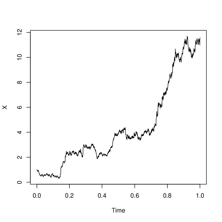
Refer to caption (a) Sample path of XX Refer to caption (b) Increment of XX
Figure 1: Sample path of XX and its increments (λ=30\lambda=30)

Table 2 shows the summary of error ratios (percentage deviation of estimated values from the true value for each estimator), and Figure 2 gives their box plots. In this case, both BV (bv) and minRV (mrv) seem to suffer from upward bias due to jumps. In particular, the BV deviates from the true value considerably. On the other hand, GRV with normalization perform well with errors concentrating around zero (grv.lgrv, grv.mrv). Note that, although WGRV performs relatively well, it seems to have a small upward bias (wgrv.lgrv, wgrv.mrv). This suggests that, if there are many large jumps, using an upper quantile (V(sn​(α))V_{(s_{n}(\alpha))}) may sometimes lead to biases rather than obtaining a robust estimate.

The three right box plots in this figure (grv[0.20], grv[0.10], grv[0.05]) are the results of GRV without normalizing increments by local-global filters, with the cut-off ratio α=0.2, 0.1, 0.05\alpha=0.2,\ 0.1,\ 0.05, respectively. We see that they seem to be less precise (especially when α\alpha is large extremely small) than GRV or WGRV with local volatility. This result suggests that, if we do not normalize increments by spot volatilities in the case of non-constant volatility, we end up obtaining inappropriate estimates.

Intuitively, when we ignore normalization, we tend to eliminate increments where volatility is high (because they are typically large), even if they come from the Brownian motion, while keeping relatively small jumps which we should actually remove. In addition, theoretically, the adjusting constant q⁡(α)q(\alpha) in the definition of GRV (2.3) comes from the standard normal distribution. Therefore, when the volatility is non-constant, we should normalize the increments |Δi​X||\Delta_{i}{\color[rgb]{0,0,0}X}| by local volatility to make them approximately standard normally distributed.

Table 2: Summary of error ratios: λ=30\lambda=30
Min. 1st Qu. Median 3rd Qu. Max.
trv[0.45] -29.88 -28.16 -27.42 -26.45 -21.64
trv[0.20] -9.40 -3.57 -1.95 -0.67 3.54
trv[0.10] 0.32 3.38 4.55 6.11 21.61
bv -0.25 2.66 3.87 5.11 8.98
mrv -2.61 0.36 1.43 2.48 5.75
grv.lgrv[0.20] -6.65 -1.03 -0.10 0.88 3.64
grv.mrv[0.20] -6.65 -1.33 -0.40 0.64 3.65
wgrv.lgrv[0.20] -3.50 -0.39 0.60 1.46 3.68
wgrv.mrv[0.20] -3.53 -0.50 0.44 1.32 3.72
grv[0.20] -9.29 -4.39 -3.21 -1.91 2.15
grv[0.10] -10.26 -2.84 -1.76 -0.76 2.71
grv[0.05] -13.85 -4.41 -1.77 -0.42 3.38
grv.lgrv.mov -9.13 -1.18 -0.00 0.95 3.55
wgrv.lgrv.mov -3.19 -0.14 0.80 1.62 4.61
Refer to caption Refer to caption
Figure 2: Error ratios [%] for the case of high intensity: λ=30\lambda=30

The good news is that they also perform well even in the case of extremely high intensity. We consider λ=50\lambda=50 here to see their accuracy. Figure 3 shows a sample path and its increments. It is obvious there are numerous jumps and one can easily imagine that the standard realized volatility estimator can never estimate the true volatility. Table 3 and Figure 4 show error ratios of each estimator for λ=50\lambda=50. It shows that GRV and WGRV with cut-off ratio α=0.2\alpha=0.2 perform well even in the case of high intensity of jumps.

Refer to caption (a) Sample path of XX Refer to caption (b) Increment of XX
Figure 3: Sample path of XX and its increments (λ=50\lambda=50)
Table 3: Summary of error ratios: λ=50,α=0.2\lambda=50,\ \alpha=0.2
Min. 1st Qu. Median 3rd Qu. Max.
trv[0.45] -99.52 -98.90 -98.52 -98.09 -94.42
trv[0.20] -52.18 -27.61 -19.86 -12.98 2.35
trv[0.10] 0.78 11.76 15.51 20.33 37.69
bv 2.71 13.60 17.47 20.89 37.19
mrv -6.36 3.40 7.72 11.58 27.20
grv.lgrv[0.20] -38.58 -7.51 -2.38 1.82 18.41
grv.mrv[0.20] -39.65 -8.54 -3.51 0.81 16.58
wgrv.lgrv[0.20] -10.64 0.87 3.99 7.44 25.22
wgrv.mrv[0.20] -12.60 -0.08 3.18 6.74 23.23
grv[0.20] -33.92 -15.51 -11.40 -7.01 5.42
grv[0.10] -56.46 -23.57 -11.63 -4.84 9.21
grv[0.05] -66.14 -40.55 -29.94 -17.97 5.88
grv.lgrv.mov -48.17 -16.03 -6.55 -0.14 16.16
wgrv.lgrv.mov -10.31 2.16 5.85 9.61 31.21
Refer to caption Refer to caption
Figure 4: Error ratios [%] for the case of high intensity: λ=50\lambda=50

By taking α\alpha larger, accuracy improves. Table 4 shows the error ratios of each estimator in the case of λ=50\lambda=50, with α=α0\alpha=\alpha_{0} ranging from 0.1 to 0.5. We can see that, for large cut-off ratio (α=α0=0.4,0.5\alpha=\alpha_{0}=0.4,0.5), GRV and WGRV with spot volatilities (grv.lgrv, grv.mrv, wgrv.lgrv, wgrv.mrv) still perform well. Looking in more detail, we see that the local GRV outperforms local minRV for both GRV and WGRV. This example imply that we should take a cut-off ratio quite large in order to obtain a precise estimate.

Table 4: Error ratios [%] for the case of extremely high intensity: λ=50\lambda=50
Cut-off ratio (α=α0\alpha=\alpha_{0})
0.1 0.2 0.3 0.4 0.5
trv[0.45] -98.40 -98.40 -98.40 -98.40 -98.40
trv[0.20] -20.35 -20.35 -20.35 -20.35 -20.35
trv[0.10] 16.19 16.19 16.19 16.19 16.19
bv 17.60 17.60 17.60 17.60 17.60
mrv 7.71 7.71 7.71 7.71 7.71
grv.lgrv[α\alpha] -18.04 -3.49 -0.41 -0.96 -1.47
grv.mrv[α\alpha] -18.05 -4.35 -2.62 -3.90 -4.89
wgrv.lgrv[α\alpha] 10.28 4.05 2.27 1.35 0.59
wgrv.mrv [α\alpha] 10.87 3.21 1.06 -0.30 -1.40
grv[0.20] -11.50 -11.50 -11.50 -11.50 -11.50
grv[0.10] -14.60 -14.60 -14.60 -14.60 -14.60
grv[0.05] -28.85 -28.85 -28.85 -28.85 -28.85
grv.lgrv.mov -8.31 -8.76 -8.78 -8.80 -8.83
wgrv.lgrv.mov 4.99 6.26 6.48 6.63 6.73

7.1.2 The case of moderate intensity: GRV with a shrinking cut-off ratio

Next, we consider the case of low intensity. In this case, we can use shrinking cut-off rate. Recall that the shrinking cut-off rate is defined by αn=⌊B​nδ1⌋/n\alpha_{n}=\lfloor Bn^{\delta_{1}}\rfloor/n. In this simulation, we set B=10B=10 and δ1=0.45\delta_{1}=0.45, so the cut-off rate is then αn=0.1525\alpha_{n}=0.1525.

The error ratios are shown in Table 5 Figure 5. All global-filtering estimators perform well (for GRVs with fixed cut-off ratio, we set α=0.2\alpha=0.2 as before). These results suggest that if there are not so many jumps in the data, it would be advisable to use as many data as possible by making the cut-off ratio small. Note that TRV still has bias, especially for ρ=0.45\rho=0.45. This implies that the accuracy of estimation is still highly vulnerable to the choice of ρ\rho for TRV, even in the case of moderate intensity of jumps.

Table 5: Summary of error ratios: λ=5\lambda=5
Min. 1st Qu. Median 3rd Qu. Max.
trv[0.45] -29.61 -27.40 -26.09 -23.89 -18.27
trv[0.20] -2.79 -0.58 0.14 0.85 3.86
trv[0.10] -2.39 1.16 2.52 4.25 13.51
bv -2.26 0.31 1.29 2.24 6.34
mrv -3.63 -0.69 0.29 1.24 4.27
grv.lgrv[0.20] -3.62 -1.44 -0.55 0.21 4.79
grv.mrv[0.20] -3.59 -1.40 -0.55 0.30 5.00
wgrv.lgrv[0.20] -3.52 -1.11 -0.39 0.44 4.55
wgrv.mrv[0.20] -3.53 -1.06 -0.40 0.46 4.62
grv[0.20] -7.14 -2.82 -1.75 -0.75 2.90
grv[0.10] -5.46 -2.15 -1.32 -0.46 3.17
grv[0.05] -4.15 -1.63 -0.86 -0.10 3.23
grv.lgrv.mov -3.54 -1.32 -0.50 0.27 4.87
wgrv.lgrv.mov -3.15 -0.96 -0.34 0.47 4.17
Refer to caption Refer to caption
Figure 5: Error ratios [%] for the case of low intensity: λ=5\lambda=5

For GRV and WGRV with shrinking cut-off ratio, we proved the asymptotic mixed normality. Hence, the distribution of the Studentized errors Γ−1/2n(𝐕n−Θ)\Gamma^{-1/2}\sqrt{n}({\bf V}_{n}-\Theta) and Γ−1/2n(𝐖n−Θ)\Gamma^{-1/2}\sqrt{n}({\bf W}_{n}-\Theta) are expected to follow the standard normally distribution.

Figure 6 shows QQ plots comparing theoretical quantiles of the standard normal distribution and the Studentized errors of GRV and WGRV estimators with shrinking threshold, BV and minRV. In this example, wgrv.lgrv.mov outperforms the others. It is close to the standard normal distribution. On the other hand, grv.lgrv.mov seems to deviate from N⁡(0,1)N(0,1). We can also see that bv are far from N⁡(0,1)N(0,1), implying that it is not appropriate even in the case of low intensity.

Refer to caption Refer to caption
Figure 6: QQ plot for Studentized errors: λ=5\lambda=5

The important tuning parameter for the shrinking threshold GRV is the exponent δ1\delta_{1}, an appropriate choice of which may strongly depend on the intensity of jumps. Recall that small δ1\delta_{1} means that we keep almost all the samples untrimmed. Table 6 shows average error ratios of GRV and WGRV with shrinking cut-off ratio for several values of intensity λ\lambda and the parameter δ1\delta_{1}. For moderate intensity (λ=5,10\lambda=5,10), the average ratios are not so large for small δ1\delta_{1}. On the other hand, for high intensity (λ=30,50\lambda=30,50), this is not the case. Indeed, as for GRV, estimation errors are quite large downward for small δ1\delta_{1}. This can be interpreted that its multiplication of q​(αn)−1q(\alpha_{n})^{-1} for GRV is insufficient to compensate its elimination of jumps (small δ1\delta_{1} implies small αn\alpha_{n}, making q​(αn)−1q(\alpha_{n})^{-1} close to 1). Moreover, as for WGRV, there occur large upward biases for small δ1\delta_{1}, since it keeps almost large increments and uses an extremely large increment for winsorization.

It is worth noting that large δ1\delta_{1} makes both GRV and WGRV accurate to a certain extent, even in the case of high intensity of jumps. Thus, in practice, one may use shrinking cut-off GRV and WGRV by setting the tuning parameter δ1\delta_{1} sufficiently close to 1/21/2.

However, as Figure 7 implies, the errors are not normally distributed as theory predicts when the intensity of jumps is extremely high. We should be aware that GRV and WGRV with shrinking cut-off may suffer from some biases in the case of extremely intensive jumps. We may consider using a large fixed cut-off ratio (as discussed in the previous subsection) in such a situation.

Refer to caption Refer to caption
Figure 7: QQ plot for Studentized errors: λ=50,δ1=0.49\lambda=50,\ \delta_{1}=0.49
Table 6: Average error ratios [%\%] of GRV and WGRV with shrinking cut-off ratio

(a) GRV

Intensity of jumps (λ\lambda)
δ1\delta_{1} 5 10 30 50
0.10 -0.41 -3.07 -23.89 -43.57
0.20 -0.28 -1.56 -18.95 -39.12
0.30 -0.58 -0.63 -11.40 -31.14
0.40 -1.22 -0.65 -2.91 -17.39
0.45 -1.57 -1.09 -0.57 -8.76
0.49 -1.82 -1.50 -0.43 -3.01

(b) WGRV

Intensity of jumps (λ\lambda)
δ1\delta_{1} 5 10 30 50
0.10 2.03 5.88 60.71 208.18
0.20 1.18 3.43 22.96 66.24
0.30 0.43 1.76 10.27 29.11
0.40 -0.32 0.60 4.30 11.13
0.45 -0.80 0.00 2.74 6.26
0.49 -1.11 -0.46 1.85 3.83

7.1.3 The case of constant volatility

Since we assumed that the volatility is location-dependent in the previous sections, the normalization by estimated spot volatilities is needed to obtain an accurate estimator. However, if the true volatility of data is constant, we may ignore normalization.

Here we set η=0\eta=0 so that the data is driven by a constant-volatility diffusion process. The intensity is λ=30\lambda=30. The summary table of estimated values are shown in Table 7. Obviously, all types of GRV and WGRV outperform other estimators.

Figure 8 shows the error ratios of this case. The GRVs without normalization (grv[0.20], grv[0.10] and grv[0.05]) perform as well as those with normalization. This suggests that, if the true process can be thought as constant-volatility, we may skip normalization (calculation of spot volatilities) procedure.

However, it would be more typical that the volatility is non-constant. Thus, basically, it would be advisable to use normalization.

Table 7: Summary table of estimated values: λ=30\lambda=30
Min. 1st Qu. Median 3rd Qu. Max.
trv[0.45] 0.41 0.44 0.45 0.46 0.49
trv[0.20] 0.97 1.11 1.16 1.22 1.45
trv[0.10] 1.67 2.49 2.76 3.08 4.81
bv 1.16 1.43 1.53 1.63 2.52
mrv 0.92 1.03 1.07 1.13 2.52
grv.lgrv[0.20] 0.94 1.01 1.05 1.07 1.17
grv.mrv[0.20] 0.94 1.02 1.05 1.09 1.32
wgrv.lgrv[0.20] 0.95 1.02 1.05 1.08 1.16
wgrv.mrv[0.20] 0.95 1.02 1.05 1.08 1.17
grv[0.20] 0.94 1.01 1.05 1.07 1.17
grv[0.10] 0.95 1.02 1.06 1.08 1.16
grv[0.05] 0.96 1.04 1.07 1.09 1.17
grv.lgrv.mov 0.95 1.02 1.05 1.08 1.16
wgrv.lgrv.mov 0.95 1.02 1.05 1.08 1.15
True Value 1.00 1.00 1.00 1.00 1.00
Refer to caption Refer to caption
Figure 8: Error ratios [%] results for the constant volatility: λ=30\lambda=30

7.2 The case of Neyman-Scott type clustering jumps

As the previous examples show, the minRV performs relatively well in the case of compound Poisson type jumps. However, even if the intensity of jumps is small, the minRV may suffer from an upward bias depending on the structure of jumps. In particular, if there are consecutive jumps (which is quite rare for compound Poisson processes), the minRV loses it advantage. Here we show an example of such a situation.

We consider the case that the data-generating process is given by X=U+JX=U+J, where UU is the continuous part and JJ is the jump part. Here we assume that JJ is a marked Neyman-Scott clustering process (simply denoted by NS hereafter), instead of a compound Poisson process.

The NS process is a typical point process representing consecutive jumps. That is, there may be jumps within some consecutive intervals. This leads to upward bias of BV and minRV because the both of two adjacent increments can consist of large jumps. The NS process is constructed as follows.

(1)

Set “centers” on the time interval [0,1][0,{\color[rgb]{0,0,0}1}] by a Poisson process (Nt0)(N_{t}^{0}) with intensity λ0\lambda_{0}. A center is defined as the point t∈[0,1]t\in[0,{\color[rgb]{0,0,0}1}] which satisfies Δ​Nt=1\Delta N_{t}=1.

(2)

For each center c∈[0,1]c\in[0,{\color[rgb]{0,0,0}1}], choose the number NcN_{c} of “children,” assuming NcN_{c} is Poisson-distributed with mean λc\lambda_{c}.

(3)

For each center c∈[0,1]c\in[0,{\color[rgb]{0,0,0}1}], generate independently and exponentially distributed random variables (vi(c))1≤i≤Nc\left(v_{i}^{(c)}\right)_{1\leq i\leq N_{c}} with mean hh. Then the location of child ii derived from center cc is defined as c−vi(c)c-v_{i}^{(c)}. This defines the location of a jump.

(4)

For each child ii, generate an independently and normally distributed random variable ξi∼N⁡(0,νJ2)\xi_{i}\sim N(0,\nu_{J}^{2}). This determines the size and direction of a jump Δ​Js\Delta J_{s}.

(5)

The NS process is defined as Jt=∑s∈[0,t]Δ​JsJ_{t}=\sum_{s\in[0,t]}\Delta J_{s}.

We generate X=U+JX=U+J, where U{\color[rgb]{0,0,0}U} is the Brownian semimartingale independent of JJ, satisfying the stochastic differential equation

d​Ut=θ​Ut​d​t+(σ+η​Ut2)14​d​wtdU_{t}=\theta\>U_{t}dt+(\sigma+\eta\>U_{t}^{2})^{\frac{1}{4}}dw_{t} (7.2)

with U0=1U_{0}=1. We set λ0=λc=5\lambda_{0}=\lambda_{c}=5 and νJ=0.5\nu_{J}=0.5. For the continuous part UU, we use θ=0.2,σ=1,η=3\theta=0.2,\ \sigma=1,\ \eta=3. As before, the number nn of samples is n=2000n=2000, and the number of trials is 500.

Table 8: Summary table of error ratios: Neyman-Scott clustering jumps
Min. 1st Qu. Median 3rd Qu. Max.
trv[0.45] -97.04 -88.67 -82.29 -75.74 -59.83
trv[0.20] -74.35 -29.07 -11.09 6.46 138.67
trv[0.10] -68.02 -14.24 3.17 24.43 157.66
bv -54.60 5.52 27.19 69.17 369.71
mrv -67.31 -1.40 19.59 61.35 300.83
grv.lgrv[0.20] -74.39 -31.45 -14.02 3.64 136.14
grv.mrv[0.20] -70.53 -26.44 -9.19 8.39 139.11
wgrv.lgrv[0.20] -74.49 -31.31 -13.35 4.32 137.83
wgrv.mrv[0.20] -74.48 -30.70 -12.73 4.23 136.96
grv[0.20] -74.89 -33.38 -16.67 0.73 134.64
grv[0.10] -74.70 -32.63 -15.03 1.88 136.44
grv[0.05] -74.38 -31.68 -14.04 3.40 136.67
grv.lgrv.mov -74.50 -31.63 -13.79 3.84 138.23
wgrv.lgrv.mov -74.32 -30.82 -12.89 4.34 139.78

Table 8 and Figure 9 show the error ratios in the case of NS jumps. Because of the possible consecutive jumps, both bipower variation and minRV have upward bias, whereas GRV and WRGV are all robust to such clustering jumps. This suggests that the GRV and WRGV perform very well for various structures of jumps.

Refer to caption
Figure 9: Error ratios [%] for the case of Neyman-Scott clustering jumps

7.3 A remark on estimation of spot volatilities

Finally, we argue how estimation of spot volatilities affect the accuracy of GRV and WGRV.

We have used κn=⌊B​nc⌋=⌊10​n0.45⌋=305\kappa_{n}=\lfloor Bn^{c}\rfloor=\lfloor 10n^{0.45}\rfloor=305 for local GRV and local minRV and seen that GRV and WGRV with these spot volatilities perform highly well. However, the choice of κn\kappa_{n} may affect the accuracy of GRV and WGRV. In fact, if the true volatility varies greatly, a wide subinterval (a large κn\kappa_{n}) leads to imprecise estimation of spot volatilities and causes misdetection of jumps by using such information. Therefore, it ends up obtaining biases of GRV and WGRV.

To see this, consider the following SDE:

d​Xt=θ​Xt​d​t+(σ+η​sin2⁡Xt)​d​wt+d​Jt,\displaystyle dX_{t}=\theta X_{t}dt+(\sigma+\eta\sin^{2}X_{t})dw_{t}+dJ_{t},

where Jt=∑j=1NtξjJ_{t}=\sum_{j=1}^{N_{t}}\xi_{j} is the same compound Poisson process with intensity λ\lambda as in Section 7.1. We set σ=1,η=5,λ=10,μ=0.3,ν=0.2\sigma=1,\eta=5,\lambda=10,\mu=0.3,\nu=0.2. Again, the number nn of samples is n=2000n=2000, and the number of trials is 500. In this example, the volatility (σ+η​sin2⁡Xt)2(\sigma+\eta\sin^{2}X_{t})^{2} swings in the range [1,36][1,36]. A sample path of this model is shown in Figure 10. The volatility alternates between low and high in short time intervals, so the estimation of spot volatility requires an appropriate choice of κn\kappa_{n}.

Refer to caption (a) Sample path of XX Refer to caption (b) Increment of XX
Figure 10: Sample path of XX and its increments

Table 9 shows the summary and average error ratios of GRV and WGRV, respectively. for several values of cc and BB that determine the width κ¯n=2​κn+1\overline{\kappa}_{n}=2\kappa_{n}+1 of subintervals for spot volatility estimation. This indicates that large BB and cc (wide subinterval) tend to give imprecise estimates. Since the volatility varies in a wide subinterval as Figure 10 shows, the estimated spot volatility is prone to deviate the true value. This leads to misdetection of jumps, and thus distorts the estimate of GRV and WGRV. For instance, an underestimated spot volatility makes normalized increments too large, so the increments are likely to be regarded as jumps and eliminated from calculation of the estimates. As a result, GRV and WGRV are underestimated. In this example, it seems that small values such as c=0.1,0.2c=0.1,0.2 and B=1,5B=1,5 are preferable.

This example suggests that we should choose the tuning parameters BB and cc carefully, especially when volatility switches between high and low states frequently. After all, the proper choice of tuning parameters, such as BB and cc, while observing the data in detail, is needed to obtain precise estimates by GRV and WGRV.

Table 9: Average error ratios of GRV and WGRV for different cc and BB determining the width κ¯n\overline{\kappa}_{n}

(a) GRV with local GRV (grv.lgrv)

BB
cc 1 5 10 20
0.10 3.41 -5.80 -9.31 -15.17
0.20 -1.19 -9.31 -15.17 -24.28
0.30 -5.26 -16.48 -26.09 -36.26
0.40 -9.31 -27.63 -37.64 -44.13
0.45 -12.36 -33.71 -42.02 -46.39
0.49 -15.46 -37.92 -44.30 -47.37

(b) GRV with local minRV (grv.mrv)

BB
cc 1 5 10 20
0.10 6.21 -4.21 -6.92 -11.85
0.20 0.69 -6.92 -11.85 -20.91
0.30 -3.85 -13.08 -22.75 -33.82
0.40 -6.92 -24.44 -35.37 -43.14
0.45 -9.33 -31.01 -40.38 -46.01
0.49 -12.11 -35.72 -43.37 -47.22

(c) WGRV with local GRV (wgrv.lgrv)

BB
cc 1 5 10 20
0.10 15.27 1.33 -3.69 -9.64
0.20 8.81 -3.69 -9.64 -17.78
0.30 1.88 -10.83 -19.33 -28.89
0.40 -3.69 -20.74 -30.20 -37.17
0.45 -6.97 -26.38 -34.80 -39.68
0.49 -9.94 -30.50 -37.36 -40.95

(d) WGRV with local minRV (wgrv.mrv)

BB
cc 1 5 10 20
0.10 22.42 3.91 -1.64 -7.54
0.20 13.26 -1.64 -7.54 -15.38
0.30 4.77 -8.71 -16.88 -26.58
0.40 -1.64 -18.29 -28.05 -35.98
0.45 -4.96 -23.98 -33.10 -39.12
0.49 -7.78 -28.37 -36.22 -40.71

8 Concluding remarks

In this paper, we construct the global realized volatility estimator in the nonparametric context. We proved the consistency and the asymptotic normality of GRV and WGRV, and, by numerical simulations, we show that these new approaches outperform previous studies which use increments within a single or two intervals.

Our new approach for eliminating jumps is highly versatile. For example, by normalization, it works well when the volatility of data is driven by a nonconstant-volatility process. Moreover, both GRV and WGRV are accurate enough in the case of not only compound-Poisson sporadic jumps but also Neyman-Scott consecutive jumps.

The global-filtering method could be extended to the covariance estimation even under the nonsynchronous sampling scheme. Furthermore, this approach could also be applied to construct a test statistic for jump. Also, it is valuable to apply our approach to empirical research of high-frequency time series data. These are important topics for future research.

References

  • [1] Andersen, T.G., Dobrev, D., Schaumburg, E.: Jump-robust volatility estimation using nearest neighbor truncation. J. Econometrics 169(1), 75–93 (2012). DOI 10.1016/j.jeconom.2012.01.011
  • [2] Barndorff-Nielsen, O.E., Shephard, N.: Power and bipower variation with stochastic volatility and jumps. Journal of Financial Econometrics 2, 1–48 (2004)
  • [3] Barndorff-Nielsen, O.E., Shephard, N., Winkel, M.: Limit theorems for multipower variation in the presence of jumps 116(5), 796–806 (2006). DOI 10.1016/j.spa.2006.01.007
  • [4] Brouste, A., Fukasawa, M., Hino, H., Iacus, S., Kamatani, K., Koike, Y., Masuda, H., Nomura, R., Ogihara, T., Shimuzu, Y., Uchida, M., Yoshida, N.: Statistical inference for stochastic processes: overview and prospects. Journal of Statistical Software 57(4), 1–51 (2014)
  • [5] Dohnal, G.: On estimating the diffusion coefficient. J. Appl. Probab. 24(1), 105–114 (1987)
  • [6] Genon-Catalot, V., Jacod, J.: On the estimation of the diffusion coefficient for multi-dimensional diffusion processes. Ann. Inst. H. Poincaré Probab. Statist. 29(1), 119–151 (1993)
  • [7] Iacus, S.M., Yoshida, N.: Simulation and inference for stochastic processes with YUIMA. Springer (2018)
  • [8] Inatsugu, H., Yoshida, N.: Global jump filters and quasi-likelihood analysis for volatility. Annals of the Institute of Statistical Mathematics, on-line (2021)
  • [9] Kamatani, K., Uchida, M.: Hybrid multi-step estimators for stochastic differential equations based on sampled data. Statistical Inference for Stochastic Processes 18(2), 177–204 (2014)
  • [10] Kessler, M.: Estimation of an ergodic diffusion from discrete observations. Scand. J. Statist. 24(2), 211–229 (1997)
  • [11] Koike, Y.: An estimator for the cumulative co-volatility of asynchronously observed semimartingales with jumps. Scandinavian Journal of Statistics 41(2), 460–481 (2014)
  • [12] Mancini, C.: Disentangling the jumps of the diffusion in a geometric jumping brownian motion 64(1), 19–47 (2001)
  • [13] Ogihara, T., Yoshida, N.: Quasi-likelihood analysis for the stochastic differential equation with jumps. Stat. Inference Stoch. Process. 14(3), 189–229 (2011). DOI 10.1007/s11203-011-9057-z. URL http://dx.doi.org/10.1007/s11203-011-9057-z
  • [14] Ogihara, T., Yoshida, N.: Quasi-likelihood analysis for nonsynchronously observed diffusion processes. Stochastic Processes and their Applications 124(9), 2954–3008 (2014)
  • [15] Prakasa Rao, B.: Statistical inference from sampled data for stochastic processes. Statistical inference from stochastic processes (Ithaca, NY, 1987) 80, 249–284 (1988)
  • [16] Prakasa Rao, B.L.S.: Asymptotic theory for nonlinear least squares estimator for diffusion processes. Math. Operationsforsch. Statist. Ser. Statist. 14(2), 195–209 (1983)
  • [17] Shimizu, Y., Yoshida, N.: Estimation of parameters for diffusion processes with jumps from discrete observations. Stat. Inference Stoch. Process. 9(3), 227–277 (2006). DOI 10.1007/s11203-005-8114-x. URL http://dx.doi.org/10.1007/s11203-005-8114-x
  • [18] Uchida, M., Yoshida, N.: Adaptive estimation of an ergodic diffusion process based on sampled data. Stochastic Process. Appl. 122(8), 2885–2924 (2012). DOI 10.1016/j.spa.2012.04.001. URL http://dx.doi.org/10.1016/j.spa.2012.04.001
  • [19] Uchida, M., Yoshida, N.: Quasi likelihood analysis of volatility and nondegeneracy of statistical random field. Stochastic Process. Appl. 123(7), 2851–2876 (2013). DOI 10.1016/j.spa.2013.04.008. URL http://dx.doi.org/10.1016/j.spa.2013.04.008
  • [20] Uchida, M., Yoshida, N.: Adaptive bayes type estimators of ergodic diffusion processes from discrete observations. Statistical Inference for Stochastic Processes 17(2), 181–219 (2014)
  • [21] Yoshida, N.: Estimation for diffusion processes from discrete observation. J. Multivariate Anal. 41(2), 220–242 (1992)
  • [22] Yoshida, N.: Polynomial type large deviation inequalities and quasi-likelihood analysis for stochastic differential equations. Ann. Inst. Statist. Math. 63(3), 431–479 (2011). DOI 10.1007/s10463-009-0263-z. URL http://dx.doi.org/10.1007/s10463-009-0263-z
  • [23] Yoshida, N.: Asymptotic expansion of a variation with anticipative weights. arXiv preprint arXiv:2101.00089 (2020)