Memory-Associated Differential Learning

Yi Luo Affiliation: School of Computer Science and Engineering, University of Electronic Science and Technology of China, Chengdu 611731, China. Email: cf020031308@163.com Aiguo Chen Note: Corresponding Author Affiliation: School of Computer Science and Engineering, University of Electronic Science and Technology of China, Chengdu 611731, China. Email: {agchen Bei Hui Affiliation: School of Information and Software Engineering, University of Electronic Science and Technology of China, Chengdu 611731, China. Email: bhui Ke Yan Affiliation: School of Computer Science and Engineering, University of Electronic Science and Technology of China, Chengdu 611731, China. Email: kyan}@uestc.edu.cn

Abstract

Conventional Supervised Learning approaches focus on the mapping from input features to output labels. After training, the learnt models alone are adapted onto testing features to predict testing labels in isolation, with training data wasted and their associations ignored. To take full advantage of the vast number of training data and their associations, we propose a novel learning paradigm called Memory-Associated Differential (MAD) Learning. We first introduce an additional component called Memory to memorize all the training data. Then we learn the differences of labels as well as the associations of features in the combination of a differential equation and some sampling methods. Finally, in the evaluating phase, we predict unknown labels by inferencing from the memorized facts plus the learnt differences and associations in a geometrically meaningfull manner. We gently build this theory in unary situations and apply it on Image Recognition, then extend it into Link Prediction as a binary situation, in which our method outperforms strong state-of-the-art baselines on ogbl-ddi dataset.

1 Introduction

Refer to caption — Figure 1: The difference between Conventional Supervised Learning and MAD Learning. The former learns the mapping from features to labels in training data and apply this mapping on testing data, while the latter learns the differences and associations among data and inferences testing labels from memorized training data.

In this work, we develop MAD Learning, Memory-Associated Differential Learning, to inference from the memorized facts that we already know to predict what we want to know. Different from conventional Supervised Learning approaches which learn the mapping from input features to output labels, our method focuses on the relationship between features and features, labels and labels. When predicting on testing features, MAD Learning inferences from similar memory and make some difference upon it to get testing labels. We illustrate this difference in Figure 1.

In Section 3.1, we gently build this theory in the unary situation. To illustrate that the existence of memory and differences are equally important, we conduct experiments with either or none of these two parts disabled in Section 4.1.1.

To have a better approximation, we investigate several techniques of sampling such as multi-heads Vaswani et al. 2017 and propose a mechanism called Soft Sentinel to softly filter out unreliable estimations. In Section 4.1.2 we examine the effectiveness of these techniques and mechanism.

We then extend MAD Learning into binary situations in Section 3.5.1 where Link Prediction Sun et al. 2011 is taken as an example. In Section 4.3 we experiment on dataset ogbl-ddi Wishart et al. 2018 from Open Graph Benchmark (OGB) Weihua Hu 2020. On ogbl-ddi, MAD Learning outperforms state-of-the-art (SotA) baselines.

Since the differential equation in MAD Learning has the form of the first-order Taylor series approximation, it gains clear interpretability in geometry. In Section 3.5.2, we visualize a social network Zachary’s Karate Club Zachary 1977 to reveal the meaning of learnt encodings.

Finally, we extend MAD Learning to ternary and multi situations to construct more complex applications such as relation predictors for Knowledge Graphs. However, due to the huge space occupation of this method, this extension remains as a theory that we place it into Section 5 as the discussion.

As a novel learning paradigm, MAD Learning opens the door for many research directions. We raise some of them in Section 6 as conclusions.

2 Related Works

Known facts to Machine Learning models are just memorized experience to human. Early in 2014, researchers in Natural Language Processing believed the internal memory a Recurrent Neural Network Mikolov et al. 2010 had so insufficient to accurately remember all the facts occurred in history, that they proposed Memory Networks Weston et al. 2015 to take advantage of historical facts by writing to and reading from External Memory. A similar idea is adopted by us but in a different way. Instead of treating External Memory as a way to add more learnable parameters to store uninterpretable hidden states, we try to memorize the facts as they are, and then learn the differences and associations between them.

Most of the experiments in this article are designed to solve Link Prediction problem that we predict whether a pair of nodes in a graph are likely to be connected, how much the weight their edge bares, or what attributes their edge should have. In such a field, two of the most popular methods are Graph Convolution Networks (GCN) Kipf and Welling 2016 and Matrix Factorization Koren et al. 2009.

The idea of GCN is that the hidden representation of a node can be aggregated from the states of itself and of its neighbours, this usually implies that connected nodes should have similar representations. However, this assumption results in over-smoothing Li et al. 2019 that the representations of nodes become nearly identical after multiple layers that they can hardly be distinguished. MAD Learning on graphs does not suffer from this issue. It has a loose constraint that the neighbours of the same node ought to have similar representations while the connected pairs do not have to. This matters when edges are directional.

Matrix Factorization is a classical algorithm used in Recommender Systems. It decomposes the adjacency matrix into the product of two matrices. Each works as a group of embeddings for nodes. Although our method is derived from a different perspective of view, we point out that Matrix Factorization can be seen as a simplification of MAD Learning with no memory and no sampling.

3 Proposed Approach

3.1 Memory-Associated Differential Learning

We assume that the output label $y$ of an instance of input features $x$ is a differentiable function $y=y(x)$ . And besides bare features $x$ with its label $y$ unknown, we also have another $x_{0}$ called reference with its output label $y_{0}$ already known.

By applying Mean Value Theorem for Definite Integrals Comenetz 2002, we can estimate the unknown $y$ with known $y_{0}$ if $x_{0}$ is close enough to $x$ :

y=y(x)=y_{0}+\int_{x_{0}}^{x}dy\approx y_{0}+(x-x_{0})\cdot y^{\prime}(x)\triangleq\hat{y}|y_{0}

In such way, we connect the current prediction tasks $y$ to the past fact $y_{0}$ , which can be stored in external memory, and convert the learning of our target function $y(x)$ to the learning of a differential function $y^{\prime}(x)$ , which in general is more accessible than the former.

In Figure 2(a), we depict how MAD Learning predict the distribution of labels by incorporating memory and the learnable differential function. The importance of these two parts is verified in Section 4.1.1.

3.2 Inferencing from Multiple References

To get a steady and accurate estimation of $y$ , we can sample $n$ references $x_{1},x_{2},\cdots,x_{n}$ to get $n$ estimations $\hat{y}|y_{1},\hat{y}|y_{2},\cdots,\hat{y}|y_{n}$ and combine them with an aggregator such as mean:

\hat{y}=\frac{1}{n}\cdot\sum\limits_{i=1}^{n}\hat{y}|y_{i}

Since the closer the reference $x_{i}$ is, the more accurate the estimation $\hat{y}|y_{i}$ it gives, we can attach a weight on each estimation inversely proportional to the distance between the reference $x_{i}$ and $x$ . Here we adopt a function Softmin derived from Softmax which rescales the inputted $d$ -dimentional array $v$ so that every element of $v$ lies in the range $[0,1]$ and all of them sum to 1:

\text{Softmin}(v_{i})=\text{Softmax}(-v_{i})=\frac{e^{-v_{i}}}{\sum\limits_{j=1}^{d}e^{-v_{j}}}

By applying Softmin we get the aggregated estimation:

\begin{cases}\hat{y}&=\frac{1}{Z}\cdot\sum\limits_{i=1}^{n}\hat{y}|y_{i}\cdot e^{-||x_{i}-x||}\\ Z&=\sum\limits_{i=1}^{n}e^{-||x_{i}-x||}\end{cases}

3.3 Soft Sentinels and Uncertainty

With Softmin, inaccurate estimations given by distant references can hardly distort the final result, if but only if nearby references exist. Otherwise, a group of distant references which gives less reliable estimations also has a summed weight of 1, the same as a group of close references.

To rectify this issue, we introduce a mechanism on top of Softmin named Soft Sentinel. A Soft Sentinel is a dummy element mixed into the array of estimations with no information (e.g. the logit is 0) but a set distance (e.g. 0).

The estimation after $k$ Soft Sentinels distant at 1 added is

\begin{cases}\hat{y}&=\frac{1}{Z}\cdot\sum\limits_{i=1}^{n}\hat{y}|y_{i}\cdot e^{-||x_{i}-x||}\\ Z&=ke^{-1}+\sum\limits_{i=1}^{n}e^{-||x_{i}-x||}\end{cases}

When Soft Sentinels involved, only estimations given by close-enough references can have most of their impacts on the final result that unreliable estimations are supressed.

Furthermore, The weight of a single Soft Sentinel distant at 0 can be viewed as a measure of uncertainty when predicting: the further the references are, the more the uncertainty is.

In Section 4.1.2, along with the comparison between mean and Softmin, we also compare the effect of Soft Sentinels.

3.4 Other Details

3.4.1 Adaptors of Position and Memory

For the sake of flexibility and performance, we usually do not use inputted features $x$ directly, but to first convert $x$ into position $f(x)$ . Besides, the training labels are not always consistent with the models’ output. For example, sometimes labels stand for discrete possibilities while the model outputs logits. To adapt to this situation, we generally wrap the memory with an adaptor function $m$ such as a one-layer MLP, getting

\hat{y}|y_{0}=m(y_{0})+(f(x)-f(x_{0}))\cdot g(x)

where $g(x)$ stands for gradient.

3.4.2 The Choice of References

We investigate four modes to choose references:

1.

Fixed. When the inputs are rich-featured (different inputs are distinguishable simply by features), we can precompute the feature distances among data and find $K$ nearest neighbours for each input as its fixed references.
2.

Random. References are sampled arbitrarily.
3.

Dynamic NN. $K$ nearest neighbours according to the distance of position $f(x)$ (not $x$ as in Fixed Mode) are selected to be references. Since $f(x)$ are dynamically changed following the updating of $f$ , this mode may require heavy computations.

When the encodings of nodes are dynamic and no features are provided, we usually adopt Random Mode in the training phase for efficiency and adopt Dynamic NN Mode in the evaluation phase for performance.

In experiments of Section 4.1 that we carry on dataset ogbl-ddi, we record both the scores in Random Mode and Dynamic NN Mode in the evaluating phase.

3.4.3 Multiple Heads

Multi-heads can be a solution when it is hard to boost performance by adding more parameters in a single structure. It applies a model in separate instances. Each instance has the potential to learn embeddings from different subspaces. So it can also be regarded as an approach of Sampling.

We implement multi-heads in MAD Learning by combining the results from separate instances with mean function.

3.5 Binary MAD Learning

3.5.1 Link Prediction

We model the relationship between a pair of nodes in a graph by extending MAD Learning into binary situations.

Like what we do in the previous section, we first assume that the relation $r$ between node $u$ and node $v$ is a differentiable function: $r=r(u,v)$ . And besides the to-predict pair $(u,v)$ , we also have another pair of nodes $(u_{0},v_{0})$ called a reference, with their relation $r_{0}$ already known.

We apply Total Derivative and Mean Value Theorem for Definite Integrals, getting:

	$\displaystyle r$	$\displaystyle=r(u,v)$
		$\displaystyle=r_{0}+\int_{(u_{0},v_{0})}^{(u,v)}dr$
		$\displaystyle=r_{0}+\int_{(u_{0},v_{0})}^{(u,v)}(\frac{\partial{r}}{\partial{u}}du+\frac{\partial{r}}{\partial{v}}dv)$
		$\displaystyle\approx r_{0}+(u-u_{0})\cdot\frac{\partial{r}}{\partial{u}}\|_{(u,v)}+(v-v_{0})\cdot\frac{\partial{r}}{\partial{v}}\|_{(u,v)}$
		$\displaystyle\triangleq\hat{r}\|r_{0}$

To simplify the above model and assure the reference $(u_{0},v_{0})$ as close to the to-predict pair $(u,v)$ as possible, we set $u_{0}=u$ or $v_{0}=v$ , meaning $(u,v)$ always shares with a common node with $r(u_{0},v_{0})$ .

When $v=v_{0}$ holds, the partial differential $\frac{\partial{r}}{\partial{u}}|_{(u,v)}$ can be regarded as the change of $r(u,v)$ after slightly moving the node $u$ to $u_{0}$ but with node $v$ fixed, as depicted in Figure 2(b).

Therefore, we may further assume $\frac{\partial{r}}{\partial{u}}|_{(u,v)}=g_{1}(v)$ if $v=v_{0}$ and $\frac{\partial{r}}{\partial{v}}|_{(u,v)}=g_{2}(u)$ if $u=u_{0}$ , making

\begin{cases}\hat{r}|r_{0}=g_{1}(v)\cdot(u-u_{0})+r_{0},&\text{if }v=v_{0}\\ \hat{r}|r_{0}=g_{2}(u)\cdot(v-v_{0})+r_{0},&\text{if }u=u_{0}\end{cases}

Here $g_{1}(\cdot)$ is destination differential function and $g_{2}(\cdot)$ is source differential function. If the edge is undirected, these two functions can be shared.

A direct application in this binary situation is to predict whether a pair of nodes in a graph are likely to be connected. We test our method on dataset ogbl-ddi from OGB and MAD Learning outperforms SotA baselines by a large margin but with fewer parameters.

3.5.2 The Geometric Meaning of MAD Learning

To reveal the meaning of the positions and gradients within MAD Learning, in Figure 3, we visualize the 2-dimensional encodings learnt from only connections in Zachary’s Karate Club, a social network representing the interaction among club members from two communities. In both plots, each member as a node is placed at her 2-dimensional position and coloured according to which group she belongs.

In the left plot, the nodes are positioned geometrically into two clusters. This implies that the positions may have enough information for downstream tasks such as Node Classification Perozzi et al. 2014. And as we discussed earlier when comparing with GCN in Section 2, connected nodes have not to be close to each other, while neighbours of the same node tend to stay in nearby positions.

In the right plot, we see each node is attached with its gradient as a vector, pointing regularly opposite to the centre. More precisely, a node’s gradient is the direction along with which other nodes become more and more ‘connectable’.

4 Experiments

If not mentioned, the following experiments ¹¹ 1 Code: https://github.com/cf020031308/mad-learning in this work use Adam Kingma and Ba 2014 as optimizers with their learning rate set to 0.005, set K = 8, run in Random Mode in the training phase and in Dynamic NN Mode in the evaluating phase, encode positions and gradients into 32-dimensional vectors, disable multi-heads, and mix Softmin with 8 Soft Sentinels distant at 1.

4.1 On Hyperparameters

In this section, we evaluate our method on the dataset ogbl-ddi from Open Graph Benchmark (OGB) to analyse hyperparameters of MAD Learning. The metric is Hits@20, the rate of true connections that are ranked higher than the 20 top-ranked but false ones.

In the training phase, we sample arbitrary pairs of nodes to construct negative samples Grover and Leskovec 2016 and compare the scores between connected pairs and negative samples with Cross-Entropy as the loss function:

L=-\sum\limits_{i=1}^{y}\log(p_{y}(i))-\sum\limits_{i=1}^{n}\log(1-p_{n}(i))

where $y$ is the number of positive samples and $n$ of negative samples, $p_{y}(i)$ is the predicted probability of the $i$ -th positive sample and $p_{n}(i)$ of the $i$ -th negative sample.

In the evaluating phase, we record the scores not only in Dynamic NN Mode but also in Random Mode.

4.1.1 Memory and Differential Functions

To measure how important the memory and the differential functions are, we experiment with different parts of MAD Learning disabled:

1.

mad. Complete MAD Learning.
2.

nograd. MAD with gradients $g_{1}(v)=g_{2}(u)=0$ . Only memory and the Softmin weights are involved.
3.

nomem. MAD with memory $r_{0}$ = 0.

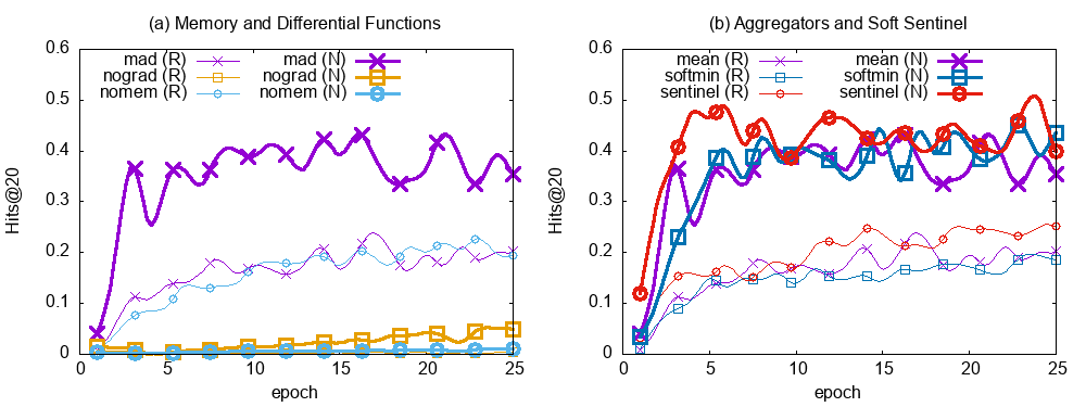
The results are depicted in Figure 4(a). The performance of the complete MAD Learning in Dynamic NN Mode significantly surpasses all others, proving that both memory and inference are indispensable.

Besides, we notice that in Random Mode, having no memory still works, because in such way the referenced nodes $u_{0}$ and $v_{0}$ can be regarded as some other pseudo nodes located at the same positions but with 0 logits to connect to $v$ or $u$ .

Furthermore, Matrix Factorization can be reduced to MAD Learning with no memory but only one fixed reference of $v$ and a pseudo node located at the origin point, as

\hat{r}=g_{1}(v)\cdot(u-0)+0=g_{1}(v)\cdot u

Another discovery is that the performance without memory in Dynamic NN Mode is far worth than in Random Mode. This is because references in Dynamic NN Mode are too close to contribute enough differences to reach the scale of predictions without memory.

4.1.2 Aggregators and Soft Sentinel

We have these three experimental settings to examine the contribution of Softmin and Soft Sentinels:

1.

mean. Estimations are aggregated by mean function.
2.

softmin. Estimations given by different references are summed up weighted by the results of Softmin applied to the distances.
3.

sentinel. Estimations of softmin with 8 Soft Sentinels at distance 1 added.

As is shown in Figure 4(b), it is no much difference between mean and Softmin. But when mixed with Soft Sentinels, MAD Learning performs better and converges faster.

4.2 Image Recognition

We conduct experiments on Image Recognition as an application of unary MAD Learning.

The datasets we use are MNIST LeCun et al. 1998, KMNIST Clanuwat et al. 2018, CIFAR-10 and CIFAR-100 Krizhevsky et al. 2009. The baselines are a two-layered convolutional neural network notated as ConvNet and ResNet18 He et al. 2015. In MAD Learning we separately use the above ConvNet or ResNet18 to extract image features before mapping them into positions and gradients. The two variances of MAD Learning with different features extractors are notated as MAD-conv and MAD-18.

Data Name	Method	#Params	Accuracy
MNIST	ConvNet	60074	98%
	MAD-conv	53982	98%
KMNIST	ConvNet	60074	94%
	MAD-conv	53982	94%
CIFAR-10	ResNet18	11181642	82%
	MAD-18	11244338	82%
CIFAR-100	ResNet18	11227812	53%
	MAD-18	11808368	50%

Table 1: Image Recognition

Method	Hits@20	#Params
MAD	0.6781	1228897
LRGA + GCN	0.6230	1576081
GCN + JKNet	0.6056	1421571
GraphSAGE	0.5390	1421057
GCN	0.3707	1289985

Table 2: Link Prediction on ogbl-ddi

We train these models for 50 epochs and record their best accuracy scores every 5 epochs, which are summarized in Table 1. As we can see, MAD Learning has no advantage in this application. We suggest that MAD Learning is better at complex tasks involving both memory and inference. Since Image Recognition is a intuitive task as “You know it when you see it”, MAD Learning can do no better than convolutional networks.

However, we repeat that MAD Learning does not predict directly. From another point of view, this experiment implies that undirect references can also be beneficial on par with direct information.

4.3 Link Prediction

We compare the performance of MAD Learning, implemented with 12 heads, 12-dimensional positions and 12-dimensional gradients, against SotA baselines from the top of the leaderboard on OGB, including GCN, GraphSAGE Hamilton et al. 2017, JKNet Xu et al. 2018, and LRGA Puny et al. 2020.

Results in Table 2 show that MAD Learning can achieve a higher Hits@20 score with fewer parameters, thus producing the new SotA.

5 Discussion

Most experiments in this work are conducted on predicting links where the relation $r$ represents a logit, but it is not difficult to explain it as edge weights. And by extending it from a scalar to a vector, MAD Learning can be used for graphs with featured edges.

We also point out that MAD Learning can learn relations in heterogeneous graphs where nodes belong to different types (usually represented by encodings in different lengths). The only requirement is that positions of the source nodes should match with gradients of the destination nodes and vice versa.

For example, in Recommender Systems, we can encode positions of users and gradients of items in 8-dimensional vectors, and encode positions of items and gradients of users in vectors with different dimensions, say 16.

For ternary relations such as head-relation-tail triplets $f=f(h,r,t)$ in Knowledge Graphs, we may also extend the binary MAD Learning into:

\begin{cases}\hat{f}|f_{0}=g_{1}(h,r)\cdot(t-t_{0})+f_{0},&\text{if }h=h_{0},r=r_{0}\\ \hat{f}|f_{0}=g_{2}(r,t)\cdot(h-h_{0})+f_{0},&\text{if }r=r_{0},t=t_{0}\\ \hat{f}|f_{0}=g_{3}(t,h)\cdot(r-r_{0})+f_{0},&\text{if }t=t_{0},h=h_{0}\end{cases}

The same extension can be made in multi situations.

6 Conclusion

In this work, we explore a novel learning paradigm which is flexible, effective and interpretable. The outstanding results, especially on Link Prediction, open the door for several research directions:

1.

The most important part of MAD Learning is memory. However, MAD Learning have to index the whole training data for random access. In Link Prediction, we implement memory as a dense adjacency matrix which results in huge occupation of space. The way to shrink memory and improve the utilization of space should be investigated in the future.
2.

Based on memory as the ground-truth, MAD Learning appends some difference as the second part. We implement this difference simply as the product of distance and differential function, but we believe there exist different ways to model it.
3.

The third part of MAD Learning is the similarity, which is used to assign weights to estimations given by different references. We reuse distance to compute the similarity, but decoupling it by some other embeddings and some other measurements such as inner product should also be worthy to explore.
4.

In this work, we do deliberately not combine direct information to focus only on MAD Learning. Since MAD Learning takes another parallel route to predict, we believe integrating MAD Learning and Conventional Supervised Learning is also a promising direction.

References

Clanuwat et al. [2018] Tarin Clanuwat, Mikel Bober-Irizar, Asanobu Kitamoto, Alex Lamb, Kazuaki Yamamoto, and David Ha. Deep learning for classical japanese literature, 2018.
Comenetz [2002] Michael Comenetz. Calculus: the elements. World Scientific Publishing Company, 2002.
Grover and Leskovec [2016] Aditya Grover and Jure Leskovec. node2vec: Scalable feature learning for networks. Jul 2016.
Hamilton et al. [2017] Will Hamilton, Zhitao Ying, and Jure Leskovec. Inductive representation learning on large graphs. In Advances in neural information processing systems, pages 1024–1034, 2017.
He et al. [2015] Kaiming He, Xiangyu Zhang, Shaoqing Ren, and Jian Sun. Deep residual learning for image recognition. Dec 2015.
Kingma and Ba [2014] Diederik P. Kingma and Jimmy Ba. Adam: A method for stochastic optimization. Dec 2014.
Kipf and Welling [2016] Thomas N. Kipf and Max Welling. Semi-supervised classification with graph convolutional networks. CoRR, abs/1609.02907, 2016.
Koren et al. [2009] Yehuda Koren, Robert Bell, and Chris Volinsky. Matrix factorization techniques for recommender systems. Computer, 42(8):30–37, 2009.
Krizhevsky et al. [2009] Alex Krizhevsky, Geoffrey Hinton, et al. Learning multiple layers of features from tiny images. 2009.
LeCun et al. [1998] Yann LeCun, Léon Bottou, Yoshua Bengio, and Patrick Haffner. Gradient-based learning applied to document recognition. Proceedings of the IEEE, 86(11):2278–2324, 1998.
Li et al. [2019] Guohao Li, Matthias Müller, Ali K. Thabet, and Bernard Ghanem. Deepgcns: Can gcns go as deep as cnns? In 2019 IEEE/CVF International Conference on Computer Vision, ICCV 2019, Seoul, Korea (South), October 27 - November 2, 2019, pages 9266–9275. IEEE, 2019.
Mikolov et al. [2010] Tomás Mikolov, Martin Karafiát, Lukás Burget, Jan Cernocký, and Sanjeev Khudanpur. Recurrent neural network based language model. In Takao Kobayashi, Keikichi Hirose, and Satoshi Nakamura, editors, INTERSPEECH 2010, 11th Annual Conference of the International Speech Communication Association, Makuhari, Chiba, Japan, September 26-30, 2010, pages 1045–1048. ISCA, 2010.
Perozzi et al. [2014] Bryan Perozzi, Rami Al-Rfou, and Steven Skiena. Deepwalk: Online learning of social representations. Mar 2014.
Puny et al. [2020] Omri Puny, Heli Ben-Hamu, and Yaron Lipman. From graph low-rank global attention to 2-fwl approximation. Jun 2020.
Sun et al. [2011] Yizhou Sun, Rick Barber, Manish Gupta, Charu C Aggarwal, and Jiawei Han. Co-author relationship prediction in heterogeneous bibliographic networks. In 2011 International Conference on Advances in Social Networks Analysis and Mining, pages 121–128. IEEE, 2011.
Vaswani et al. [2017] Ashish Vaswani, Noam Shazeer, Niki Parmar, Jakob Uszkoreit, Llion Jones, Aidan N. Gomez, Lukasz Kaiser, and Illia Polosukhin. Attention is all you need. Jun 2017.
Weihua Hu [2020] Marinka Zitnik Yuxiao Dong Hongyu Ren Bowen Liu Michele Catasta Jure Leskovec Weihua Hu, Matthias Fey. Open graph benchmark: Datasets for machine learning on graphs. arXiv preprint arXiv:2005.00687, 2020.
Weston et al. [2015] Jason Weston, Sumit Chopra, and Antoine Bordes. Memory networks. In Yoshua Bengio and Yann LeCun, editors, 3rd International Conference on Learning Representations, ICLR 2015, San Diego, CA, USA, May 7-9, 2015, Conference Track Proceedings, 2015.
Wishart et al. [2018] David S Wishart, Yannick D Feunang, An C Guo, Elvis J Lo, Ana Marcu, Jason R Grant, Tanvir Sajed, Daniel Johnson, Carin Li, Zinat Sayeeda, et al. Drugbank 5.0: a major update to the drugbank database for 2018. Nucleic acids research, 46(D1):D1074–D1082, 2018.
Xu et al. [2018] Keyulu Xu, Chengtao Li, Yonglong Tian, Tomohiro Sonobe, Ken-ichi Kawarabayashi, and Stefanie Jegelka. Representation learning on graphs with jumping knowledge networks. arXiv preprint arXiv:1806.03536, 2018.
Zachary [1977] Wayne W Zachary. An information flow model for conflict and fission in small groups. Journal of anthropological research, 33(4):452–473, 1977.