Bayesian Knockoff Filter

Consider a dataset D with $n$ independent and identically distributed (i.i.d.) observations $(\textbf{x}_{i},y_{i}),i=1,\ldots,n$, where $\textbf{x}_{i}$ and $y_{i}$ are copies of feature vector $\textbf{X}=(X_{1},\ldots,X_{p})^{\mathsf{T}}\in\mathbb{R}^{p}$ and response variable $Y\in\mathbb{R}$ respectively. It is assumed that response $Y$ only depends on a relatively small subset of features. Conditional on this subset of important features, $Y$ is independent of the remaining features. Specifically, there are two disjoint subsets of features, $\mathcal{H}_{0}$ (null set) and $\mathcal{H}_{1}$ (non-null set), satisfying that

• (i)

  $\mathcal{H}_{0}\cup\mathcal{H}_{1}=\{1,\ldots,p\}$;

• (ii)

  $\forall j\in\mathcal{H}_{0}$, $X_{j}\perp Y|\textbf{X}_{-j}$, where $\perp$ represents independence between two variables;

• (iii)

  $\forall j\in\mathcal{H}_{1}$, $X_{j}\not\perp Y|\textbf{X}_{-j}$, where $\not\perp$ represents not independence between two variables;

where $\textbf{X}_{-j}=(X_{1},\ldots,X_{j-1},X_{j+1},\ldots,X_{p})^{\mathsf{T}}$. The set $\mathcal{H}_{1}$ contains all the non-null features that have important effects on response ${Y}$, while all the null features in $\mathcal{H}_{0}$ are irrelevant to the response given the other features. Based on the observed data $\textbf{D}=\{(\textbf{x}_{i},y_{i}):i=1,\ldots,n\}$, our goal is to obtain an estimator $\hat{\mathcal{S}}$ of the non-null set $\mathcal{H}_{1}$ so that:

• (a)

  The false discovery rate (FDR),

  $$\text{FDR}=\mathbb{E}\Bigg(\frac{|\hat{\mathcal{S}}\cap\mathcal{H}_{0}|}{|\hat{\mathcal{S}}|\vee 1}\Bigg),$$

  (1)

  is controlled under a desired level $\alpha$.

• (b)

  The number of true discoveries, $|\hat{\mathcal{S}}\cap\mathcal{H}_{1}|$, is as large as possible, where $|\cdot|$ represents the size of a set.

In the framework of hypothesis testing, we are interested in testing the null hypotheses

by constructing a multiple testing procedure on $H_{01},\ldots,H_{0p}$ with a controlled FDR. The FDR (1) is analogous to the type I error rate in traditional single hypothesis testing, while a larger size of the joint set $\hat{\mathcal{S}}\cap\mathcal{H}_{1}$ implies higher power in testing hypotheses (2). By assuming a generalized linear model (GLM) $h(Y|\textbf{X};\boldsymbol{\beta},\boldsymbol{\phi})$ for the conditional distribution $f(Y|\textbf{X})$, we have

with a link function $g(\cdot)$. Thus, testing the null hypothesis $H_{0j}$ is equivalent to testing $H^{*}_{0j}:\beta_{j}=0$ for $j=1,\ldots,p$ under the GLM, which is equivalent to conducting variable selection on features $X_{1},\ldots,X_{p}$ (Candès et al., 2018).

Various methods have been proposed in the literature for multiple testing on hypotheses $H_{01},\ldots,$ $H_{0p}$ under the GLM. Existing methods can be classified into two popular paradigms. One is variable selection in regression analysis under both frequentist and Bayesian frameworks. Frequentist methods in this class include step-wise regression (Efroymson, 1960) and penalized regression methods with different penalty functions, such as ridge regression, Lasso (Tibshirani, 1996), SCAD (Fan and Li, 2001) and their variants. By fitting a GLM to $(\textbf{X},Y)$ with penalties or step-wise selection procedures to enhance sparsity on $\beta_{1},\ldots,\beta_{p}$, we can obtain the estimator $\hat{\mathcal{S}}=\{j:\hat{\beta}_{j}\neq 0\}$ for the set of non-null features. Although the asymptotic guarantees of these methods, such as model selection consistency, have been established even under high-dimensional settings, they still suffer an uncontrollable FDR with finite sample size. Bayesian variable selection approaches, such as the spike-and-slab prior (Mitchell and Beauchamp, 1988), Bayesian Lasso (Park and Casella, 2008), the horseshoe estimator (Carvalho et al., 2010) and the recent iterative Bayesian stepwise selection (IBSS) procedure (Wang et al., 2020), compute the posterior distribution of $\mathcal{H}_{1}$ and yield the Bayesian estimator $\hat{\mathcal{S}}$ by minimizing a particular posterior expected loss. However, commonly used Bayesian estimators $\hat{\mathcal{S}}$, including the highest probability model and the median probability model, do not take the FDR into consideration and hence their control of false discoveries are questionable.

Following the multiple testing procedure (Benjamini and Hochberg, 1995), another class of approaches (Sarkar and Chang, 1997; Yekutieli and Benjamini, 2001; Leek and Storey, 2008) calculate $p$-value for each hypothesis $H_{0j}$ ($j=1,\ldots,p$) or equivalently $H^{*}_{0j}$, which is only feasible under low-dimensional GLMs. Moreover, these methods can only control the FDR theoretically when these $p$-values possess an independent property or positive regression dependency on a subset (Yekutieli and Benjamini, 2001), which is difficult to verify under GLMs. To overcome such shortcomings of frequentist multiple testing procedures, Bayesian methods have been developed to control the Bayesian FDR (Storey, 2002; Whittemore, 2007) for multiple comparisons (Scott and Berger, 2006; Miranda-Moreno et al., 2007; Efron, 2008). We incorporate the recently developed knockoff methods (Barber and Candès, 2015; Candès et al., 2018) to Bayesian multiple testing procedures and develop a fully Bayesian approach with Gibbs sampled knockoffs for feature selection.

To control the finite-sample FDR in feature selection, Barber and Candès, 2015 propose a (fixed-X) knockoff filter to estimate $\mathcal{H}_{1}$ without imposing any assumptions on dependency structures among features $X_{1},\ldots,X_{p}$ under a linear model,

where features are assumed to be fixed. In contrast, the model-X knockoff filter (Candès et al., 2018) makes an extension by assuming the distribution $f(\textbf{X})$ to be known but $f(Y|\textbf{X})$ unknown. With the distribution of features $f(\textbf{X})$, a joint model $f(\textbf{X},\tilde{\textbf{X}})$ satisfying the following Definition 1 is constructed and the model-X knockoff variables $\tilde{\mathbb{X}}=(\tilde{\textbf{x}}_{1},\ldots,\tilde{\textbf{x}}_{n})^{\mathsf{T}}$ are generated conditional on the observed features $\mathbb{X}=({\textbf{x}}_{1},\ldots,{\textbf{x}}_{n})^{\mathsf{T}}$.

If $f({\bf X})$ is unknown, Candès et al., 2018 provide an approximate construction on the basis of the first two moments of features with a graphical Lasso estimator of the covariance matrix. That is, a Gaussian graphical model is fitted to features $\mathbb{X}=({\textbf{x}}_{1},\ldots,{\textbf{x}}_{n})^{\mathsf{T}}$ and the joint model $f({\bf X},\tilde{{\bf X}})$ is constructed based on the fitted graphical model. Barber and Candès, 2019 further incorporate a screening procedure prior to implementation of the knockoff filter to make it feasible in high-dimensional settings. Dai and Barber, 2016; Katsevich and Sabatti, 2019 extend the knockoff method in a way that prior knowledge of group structures among features can be utilized in feature selection and the FDR can be controlled at both the feature level and group level.

With the knockoff sample $\tilde{\mathbb{X}}$, the model-X knockoff filter computes feature statistics $W_{1},\ldots,W_{p}$ to evaluate the evidence in D against hypotheses $H_{01},\ldots,H_{0p}$. As suggested by Candès et al., 2018, $W_{j}$ should satisfy the flip-sign property under swapping of the $j$-th feature with its knockoff. Typical ways to construct feature statistics $W_{1},\ldots,W_{p}$ include the Lasso signed max (Barber and Candès, 2015) and Lasso coefficient-difference (Candès et al., 2018) statistic. A large value of $W_{j}$ usually implies strong evidence in D against $H_{0j}$. The estimator $\hat{\mathcal{S}}$ is then obtained as $\{j:W_{j}\geq\tau\}$ where the threshold $\tau$ is chosen as

where the estimator of the false discovery proportion

is shown to overestimate the overall FDR for all $t\in(0,\infty)$ (Candès et al., 2018).

However, all the aforementioned knockoff filters are frequentist methods and their inferences are based on one knockoff sample $\tilde{\mathbb{X}}$ only. Because $\widehat{\text{FDP}}(t)$ overestimates FDR, it is a conservative way to control the overall FDR by adopting the estimator of FDP, and the inference is highly dependent on the quality of the generated knockoff sample. With a low-quality $\tilde{\mathbb{X}}$, such procedures may incur power loss. In addition, all the methods rely on the assumption that the dimension of the feature vector ($p$) is large, so that the selection procedures force the size of $\hat{\mathcal{S}}$ to be zero or not smaller than $\lfloor 1/\alpha\rfloor$ if nonzero. This property results in power loss when the size of the true $\mathcal{H}_{1}$ is small. Up to now, the two problems have only been partially resolved by multi-knockoffs (Gimenez and Zou, 2019) at the cost of power loss for large $\mathcal{H}_{1}$.

To overcome the weaknesses of existing knockoff filters, we develop the Bayesian knockoff filter (BKF). Similar to the model-X knockoff filter, we assume the distribution $f(\textbf{X})$ is known and establish the joint distribution $f(\textbf{X},\tilde{\textbf{X}})$ which is invariant to swaps for all subsets $\mathcal{S}\subset\{1,\ldots,p\}$. For example, if the original X follows a multivariate Gaussian distribution $\text{MVN}(\mathbf{0},\boldsymbol{\Sigma})$, the joint distribution $f(\textbf{X},\tilde{\textbf{X}})$ satisfying Definition 1 is

where the diagonal matrix $\text{diag}\{\textbf{s}\}$ satisfies the condition that $2\text{diag}\{\textbf{s}\}-\text{diag}\{\textbf{s}\}\boldsymbol{\Sigma}\text{diag}\{\textbf{s}\}$ is a positive semi-definite matrix (Barber and Candès, 2015).

In the case of Gaussian covariates, (7) can be used to construct knockoff variables. However, if covariates are non-Gaussian or even not continuous, it is challenging to deduce the joint distribution $f(\textbf{X},\tilde{\textbf{X}})$. Although there are several existing methods to generate $\tilde{\textbf{X}}$ without an explicit expression of $f(\textbf{X},\tilde{\textbf{X}})$ (Sesia et al., 2019; Bates et al., 2020), they rely on either a specific structure of $f(\textbf{X})$ (e.g., a hidden Markov model or a graphical model) or a computational strategy (multiple-try Metropolis). If the distribution of the original X is unknown, we require $(\textbf{X},\tilde{\textbf{X}})_{{\rm Swap}(\mathcal{S})}$ and $(\textbf{X},\tilde{\textbf{X}})$ to have the same first two moments rather than the same distribution for any subset $\mathcal{S}$. We adopt the second-order approximation construction in Candès et al., 2018 to approximate $f(\textbf{X})$ with a Gaussian model $\text{MVN}(\hat{\boldsymbol{\mu}},\hat{\boldsymbol{\Sigma}})$ with the estimated mean $\hat{\boldsymbol{\mu}}$ and covariance matrix $\hat{\boldsymbol{\Sigma}}$ to construct the joint distribution $f(\textbf{X},\tilde{\textbf{X}})$. As a result, the conditional generative model $f(\tilde{\textbf{X}}|\textbf{X})$ can be deduced.

Under the GLM assumption (3) for $f(Y|\textbf{X})$, we parameterize the extended conditional distribution $f(Y|\textbf{X},\tilde{\textbf{X}})$ as an extended GLM $h(Y|\textbf{X},\tilde{\textbf{X}};\boldsymbol{\beta},\tilde{\boldsymbol{\beta}},\boldsymbol{\phi})$ with

where $\boldsymbol{\phi}$ represents nuisance parameters, such as variance $\sigma^{2}$ in a normal distribution or the dispersion parameter in an over-dispersed Poisson distribution (Nelder and Wedderburn, 1972). In the Bayesian paradigm, if the prior distribution is denoted by $f(\boldsymbol{\beta},\tilde{\boldsymbol{\beta}},\boldsymbol{\phi})$, the joint posterior density of knockoff variables and parameters is given by

Analogous to the existing frequentist work, our goal is to obtain a Bayesian estimator $\hat{\mathcal{S}}$ for the set of non-null features $\mathcal{H}_{1}$ with the Bayesian FDR controlled and the posterior expected number of true discoveries as large as possible. However, under the Bayesian paradigm, the sets $\mathcal{H}_{1}$ and $\mathcal{H}_{0}$ are both assumed to be random and thus the Bayesian FDR of any subset $\mathcal{S}$ is defined as follows.

If the posterior probabilities ${\mathbb{P}}(H_{01}|\textbf{D}),\ldots,{\mathbb{P}}(H_{0p}|\textbf{D})$ are known, it is clear that

As a result, we can obtain an equivalent definition of the Bayesian FDR for all possible ${\mathcal{S}}\subset\{1,\ldots,p\}$ as

and estimating $\mathcal{H}_{1}$ can be translated into a decision problem to select a subset,

where the loss function $L(\mathcal{H}_{1},{\mathcal{S}})=-|{\mathcal{S}}\cap\mathcal{H}_{1}|$. Under the Bayesian paradigm, the importance of feature $X_{j}$ is characterized by the posterior probability $\mathbb{P}(H_{1j}|\textbf{D})$, and minimizing the posterior expected loss $E[L(\mathcal{H}_{1},{\mathcal{S}})|\textbf{D}]=-\sum_{j\in{\mathcal{S}}}\mathbb{P}(H_{1j}|\textbf{D})$ is equivalent to maximizing the overall importance of features in the subset $\mathcal{S}$. Following the equivalent definition (11) and $\mathbb{P}(H_{1j}|\textbf{D})=1-\mathbb{P}(H_{0j}|\textbf{D})$, when posterior probabilities $\mathbb{P}(H_{0j}|\textbf{D})$ ($j=1,\ldots,p$) are known, the constrained optimization problem can be viewed as a knapsack problem to include as many features in $\hat{\mathcal{S}}$ as possible while keeping ${{\text{BFDR}}}({\mathcal{S}})\leq\alpha$, whose solution can be easily obtained via a greedy selection algorithm described in Algorithm 1.

As shown by Müller et al., 2004, Algorithm 1 is optimal in the sense that it maximizes the statistical power while controlling the Bayesian FDR under $\alpha$.

However, when the prior does not possess a point mass at $\beta_{j}=0$, posterior probabilities $\mathbb{P}(\beta_{j}=0|\textbf{D})$ ($j=1,\ldots,p$) equal $0$ for all possible observed data D and thus cannot be used for meaningful inference. Alternatively, we use a set of random variables with the flip-sign property to compute the approximate upper bounds of $\mathbb{P}(H_{0j}|\textbf{D})$ ($j=1,\ldots,p$) under the posterior density (9) by restating the flip-sign property in the Bayesian framework as follows.

Given the definition of model-X knockoff, Theorem 1 offers us a way to construct a family of random variables which obey the flip-sign property.

The proof of Theorem 1 is provided in Appendix A. Based on Theorem 1 and antisymmetric feature statistics $W_{1},\ldots,W_{p}$, the Bayesian estimator $\hat{\mathcal{S}}$ can be obtained via the greedy selection algorithm (Algorithm 1) with $\hat{\mathbb{P}}(H_{01}|\textbf{D}),\ldots,\hat{\mathbb{P}}(H_{0p}|\textbf{D})$, which are the upper bounds of ${\mathbb{P}}(H_{01}|\textbf{D}),\ldots,{\mathbb{P}}(H_{0p}|\textbf{D})$ estimated as follows.

With the marginal prior $f(\boldsymbol{\beta},\tilde{\boldsymbol{\beta}})$ invariant to swaps, the posterior distribution of $W_{j}$ is symmetric with respect to $0$ conditional on $H_{0j}$,

for $j=1,\ldots,p$. By the law of total probability, we have

If antisymmetric $W_{j}$ is well defined so that $\mathbb{P}(W_{j}>0|\textbf{D},H_{1j})>\mathbb{P}(W_{j}<0|\textbf{D},H_{1j})$ and (13) holds, we can subtract (14a) from (14b), which leads to

Due to the fact that $0<\mathbb{P}(W_{j}>0|\textbf{D},H_{1j})-\mathbb{P}(W_{j}<0|\textbf{D},H_{1j})\leq 1$, an upper bound of $\mathbb{P}(H_{0j}|\textbf{D})$ can be obtained as

We list some examples of marginal priors that are invariant to swaps and antisymmetric $W_{j}$ that satisfies $\mathbb{P}(W_{j}>0|\textbf{D},H_{1j})>\mathbb{P}(W_{j}<0|\textbf{D},H_{1j})$ and thus leads to inequality (16).

• •

  Invariant prior:

  1. 1.

     Flat prior: $f(\boldsymbol{\beta},\tilde{\boldsymbol{\beta}})\propto 1$;

  2. 2.

     Normal prior: $f(\boldsymbol{\beta},\tilde{\boldsymbol{\beta}})\propto\prod_{j=1}^{p}\exp\{-(\beta_{j}^{2}+\tilde{\beta}_{j}^{2})/(2\sigma_{j}^{2})\}$;

  3. 3.

     Laplace prior: $f(\boldsymbol{\beta},\tilde{\boldsymbol{\beta}})\propto\prod_{j=1}^{p}\exp\{-\lambda_{j}|\beta_{j}|-\lambda_{j}|\tilde{\beta}_{j}|\}$;

  4. 4.

     Modified spike-and-slab prior (Candès et al., 2018):

     $\displaystyle f(\boldsymbol{\beta},\tilde{\boldsymbol{\beta}})=\prod_{j=1}^{p}f(\beta_{j},\tilde{\beta}_{j}),\ \ \text{ where }f(\beta_{j},\tilde{\beta}_{j})=\begin{cases}I[\beta_{j}=\tilde{\beta}_{j}=0]&\text{w.p. }(1-\xi),\\ \phi(\beta_{j};0,\tau^{2})I[\tilde{\beta}_{j}=0]&\text{w.p. }\xi/2,\\ \phi(\tilde{\beta}_{j};0,\tau^{2})I[{\beta}_{j}=0]&\text{w.p. }\xi/2.\\ \end{cases}$

     (17)

• •

  Antisymmetric $W_{j}$:

  1. 1.

     $W_{j}=|\beta_{j}|-|\tilde{\beta}_{j}|$ or $W_{j}=|\beta_{j}|^{2}-|\tilde{\beta}_{j}|^{2}$;

  2. 2.

     $W_{j}=|\beta_{j}+\tilde{\beta}_{j}|\cdot sign(|\beta_{j}|-|\tilde{\beta}_{j}|)$.

In practice, with posterior samples $(\tilde{\mathbb{X}}^{(t)},\boldsymbol{\beta}^{(t)},\tilde{\boldsymbol{\beta}}^{(t)},\boldsymbol{\phi}^{(t)})$ drawn from MCMC algorithms (detailed in Section 3.3), $\textbf{W}^{(t)}=(W_{1}^{(t)},\ldots,W_{p}^{(t)})^{\mathsf{T}}$ can be computed for $t=1,\ldots,T$ and thus the upper bounds (16) can be estimated by

Following (9), Algorithm 2 provides a Gibbs sampling framework to draw posterior samples
$\{(\tilde{\mathbb{X}}^{(t)},\boldsymbol{\beta}^{(t)},\tilde{\boldsymbol{\beta}}^{(t)},\boldsymbol{\phi}^{(t)}):t=1,\ldots,T\}$, from the full conditional distributions.

In practice, the sampling of $\boldsymbol{\beta}$, $\tilde{\boldsymbol{\beta}}$, $\boldsymbol{\phi}$ and $\tilde{\textbf{x}}_{i}$ corresponding to steps 4–7 can be implemented by existing computational methods, such as Metropolis–Hasting or rejection sampling algorithms (Sesia et al., 2019; Bates et al., 2020). For example, if the joint distribution $f(\textbf{X},\tilde{\textbf{X}})$ is (7) and the extended conditional distribution $f(Y|\textbf{X},\tilde{\textbf{X}})$ is

where the nuisance parameter ($\boldsymbol{\phi}$) is the variance parameter $\sigma^{2}$, the joint posterior distribution (9) becomes

where $\textbf{x}_{i}=(x_{i1},\ldots,x_{ip})^{\mathsf{T}}$ and $\tilde{\textbf{x}}_{i}=(\tilde{x}_{i1},\ldots,\tilde{x}_{ip})^{\mathsf{T}}$ for $i=1,\ldots,n$. Let $\boldsymbol{\beta}_{-j}=(\beta_{1},\ldots,\beta_{j-1},\beta_{j+1},\ldots,\beta_{p})^{\mathsf{T}}$, $\tilde{\boldsymbol{\beta}}_{-j}=(\tilde{\beta}_{1},\ldots,\tilde{\beta}_{j-1},\tilde{\beta}_{j+1},\ldots,\tilde{\beta}_{p})^{\mathsf{T}}$ for $j=1,\ldots,p$. When the modified spike-and-slab prior (17) is used, the posterior samples of $\boldsymbol{\beta}$, $\tilde{\boldsymbol{\beta}}$, $\sigma^{2}$ and $\tilde{\textbf{x}}_{i}$ can be drawn from their full conditionals detailed in Algorithm 3.

To investigate whether the posterior samples $\tilde{\mathbb{X}}^{(1)},\ldots,\tilde{\mathbb{X}}^{(T)}$ generated by Algorithm 2 satisfy Definition 1, we apply Algorithm 2 to the data generated under settings in Section 4.1.1 (with sample size $n=1000$ and signal strength $a=2$) and compute the statistic

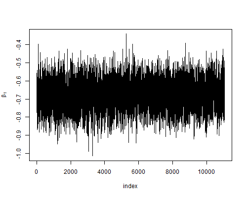
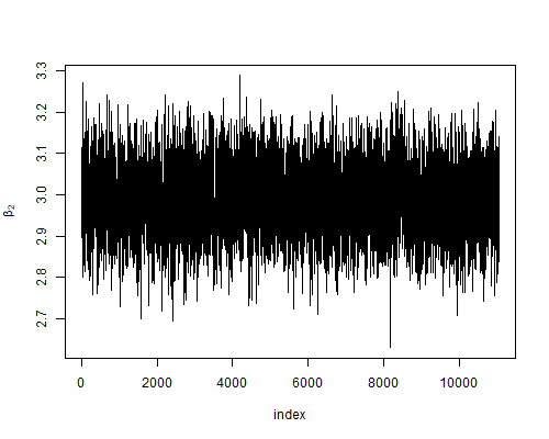
Because it is required $E[\Delta(\tilde{\mathbb{X}})]=0$ for valid knockoffs, $\Delta(\mathbb{X},\tilde{\mathbb{X}})$ would fluctuate around $0$ if knockoff variables $\tilde{\mathbb{X}}$ generated by Algorithm 2 are valid. In our experiments, we keep $T=10,000$ posterior samples after 1,000 burn-in iterations. As shown in Figure 1, the Markov chains are stable, well mixed and $\Delta(\mathbb{X},\tilde{\mathbb{X}})$ fluctuates around $0$, indicating that $\tilde{\mathbb{X}}^{(1)},\ldots,\tilde{\mathbb{X}}^{(T)}$ are valid knockoff variables.

Although the BKF is developed along the inspiring idea of knockoffs (Barber and Candès, 2015), we elaborate on its differences from existing methods as follows.

• -

  Model-X knockoff (Candès et al., 2018): In contrast to the fixed-X knockoff (Barber and Candès, 2015) which assumes that $f(Y|\textbf{X})$ is fully known as a linear model while the distribution of covariates $f(\textbf{X})$ is unknown, our method follows a similar setup of the model-X knockoff with the assumption that $f(\textbf{X})$ is known and a GLM is suitable for the conditional distribution $f(Y|\textbf{X})$. However, there are fundamental differences between the model-X knockoff and our BKF. The model-X knockoff is a frequentist method, which relies upon only one set of knockoff variables. It uses the Bayesian variable selection (BVS) method as one of possible ways to compute feature statistics and still controls the frequentist FDR in feature selection. Due to the usage of BVS feature statistics, it can leverage prior knowledge via the probability point mass at $\beta_{j}=0$ in the prior specification. In contrast, our BKF is a fully Bayesian data augmentation approach where the observed data D are treated as fixed while the set of non-null features $\mathcal{H}_{1}$, knockoffs $\tilde{\textbf{x}}_{1},\ldots,\tilde{\textbf{x}}_{n}$ and parameters $\boldsymbol{\beta},\tilde{\boldsymbol{\beta}},\boldsymbol{\phi}$ are all treated as random. Incorporating the knockoffs as missing data and FDR into a Bayesian framework, our BKF repeatedly samples knockoff variables in MCMC for more stable inference and conducts feature selection based on the Bayesian FDR control, no matter whether the priors have a point mass at $\beta_{j}=0$.

• -

  Metropolized knockoff sampling (Bates et al., 2020): Although Bates et al., 2020 use MCMC as a mechanism to generate knockoff variables, the Metropolized knockoff sampling is still a frequentist method, relying upon only one set of knockoff variables for inference. In contrast, our BKF treats knockoff variables as missing data and continuously samples them via data augmentation in MCMC for more stable Bayesian inference.

• -

  Multiple knockoffs (Gimenez and Zou, 2019): The multiple knockoffs generate more than one set of knockoff variables. Taking the 2 multi-knockoffs under a Gaussian case as an example, the joint model of original features X and knockoff features $(\tilde{\textbf{X}}_{1},\tilde{\textbf{X}}_{2})$ in Gimenez and Zou, 2019 is exchangeable for any generalized swaps among the three sets of features. Because exchangeability is assumed simultaneously across X and multiple knockoffs, this would make X and all knockoffs similar and thus lower the power. In contrast, we only define the joint model of the original features X and one set of posterior sampled knockoff features at a time for each posterior iteration in the MCMC. It requires exchangeability for any swaps between the original features and that set of knockoff features. As a result, the difference between original features and knockoff features would be greater in BKF, which leads to higher power, especially when strong correlations exist among original features.

We first compare the performance of BKF with three existing knockoff methods, including the fixed-X knockoff (Barber and Candès, 2015), the model-X knockoff (Candès et al., 2018) and the multi-knockoffs (Gimenez and Zou, 2019). For multi-knockoffs, we use the 2 multi-knockoffs in the experiments. For all the existing methods, we use their SDP (semidefinite program) constructions of knockoff and the Lasso coefficient difference as the importance statistic for inference. To evaluate the performances of different methods, two criteria are considered: (a) the overall FDR defined by (1); and (b) statistical power $|\hat{\mathcal{S}}\cap\mathcal{H}_{1}|\big/|\mathcal{H}_{1}|$, where $\hat{\mathcal{S}}$ corresponds to the estimator obtained by each of the knockoff methods in each replication. We consider different settings to examine the effects of sample size, signal strength, variance structures among features, dimensionality and the size of $\mathcal{H}_{1}$. In addition, we also evaluate the robustness of BKF and existing knockoff methods to misspecification of $f(\textbf{X})$.

For fair comparison between our BKF with existing frequentist methods, we use the flat prior in the implementation of BKF. We discard the first 500 iterations as burn-ins and keep $T=2,000$ posterior samples for inference.

References

- Barber and Candès, (2015) Barber, R. F. and Candès, E. J. (2015). Controlling the false discovery rate via knockoffs. The Annals of Statistics, 43(5):2055–2085.
- Barber and Candès, (2019) Barber, R. F. and Candès, E. J. (2019). A knockoff filter for high-dimensional selective inference. The Annals of Statistics, 47(5):2504–2537.
- Bates et al., (2020) Bates, S., Candès, E., Janson, L., and Wang, W. (2020). Metropolized knockoff sampling. Journal of the American Statistical Association, pages 1–15.
- Benjamini and Hochberg, (1995) Benjamini, Y. and Hochberg, Y. (1995). Controlling the false discovery rate: a practical and powerful approach to multiple testing. Journal of the Royal Statistical Society: Series B (Methodological), 57(1):289–300.
- Blanchard and Roquain, (2009) Blanchard, G. and Roquain, E. (2009). Adaptive false discovery rate control under independence and dependence. J. Mach. Learn. Res., 10:2837–2871.
- Candès et al., (2018) Candès, E., Fan, Y., Janson, L., and Lv, J. (2018). Panning for gold: ‘model-X’ knockoffs for high dimensional controlled variable selection. Journal of the Royal Statistical Society: Series B (Statistical Methodology), 80(3):551–577.
- Carvalho et al., (2010) Carvalho, C. M., Polson, N. G., and Scott, J. G. (2010). The horseshoe estimator for sparse signals. Biometrika, 97(2):465–480.
- Dai and Barber, (2016) Dai, R. and Barber, R. (2016). The knockoff filter for FDR control in group-sparse and multitask regression. In Balcan, M. F. and Weinberger, K. Q., editors, Proceedings of The 33rd International Conference on Machine Learning, volume 48 of Proceedings of Machine Learning Research, pages 1851–1859, New York, New York, USA. PMLR.
- Efron, (2008) Efron, B. (2008). Microarrays, empirical bayes and the two-groups model. Statistical Science, 23(1):1–22.
- Efroymson, (1960) Efroymson, M. A. (1960). Multiple regression analysis. Mathematical Methods for Digital Computers, pages 191–203.
- Fan and Li, (2001) Fan, J. and Li, R. (2001). Variable selection via nonconcave penalized likelihood and its oracle properties. Journal of the American Statistical Association, 96(456):1348–1360.
- Gimenez et al., (2019) Gimenez, J. R., Ghorbani, A., and Zou, J. (2019). Knockoffs for the mass: new feature importance statistics with false discovery guarantees. In Chaudhuri, K. and Sugiyama, M., editors, Proceedings of Machine Learning Research, volume 89 of Proceedings of Machine Learning Research, pages 2125–2133. PMLR.
- Gimenez and Zou, (2019) Gimenez, J. R. and Zou, J. (2019). Improving the stability of the knockoff procedure: multiple simultaneous knockoffs and entropy maximization. In Chaudhuri, K. and Sugiyama, M., editors, Proceedings of Machine Learning Research, volume 89 of Proceedings of Machine Learning Research, pages 2184–2192. PMLR.
- Katsevich and Sabatti, (2019) Katsevich, E. and Sabatti, C. (2019). Multilayer knockoff filter: controlled variable selection at multiple resolutions. The Annals of Applied Statistics, 13(1):1–33.
- Leek and Storey, (2008) Leek, J. T. and Storey, J. D. (2008). A general framework for multiple testing dependence. Proceedings of the National Academy of Sciences, 105(48):18718–18723.
- Miranda-Moreno et al., (2007) Miranda-Moreno, L. F., Labbe, A., and Fu, L. (2007). Bayesian multiple testing procedures for hotspot identification. Accident Analysis Prevention, 39(6):1192–1201.
- Mitchell and Beauchamp, (1988) Mitchell, T. J. and Beauchamp, J. J. (1988). Bayesian variable selection in linear regression. Journal of the American Statistical Association, 83(404):1023–1032.
- Müller et al., (2004) Müller, P., Parmigiani, G., Robert, C., and Rousseau, J. (2004). Optimal sample size for multiple testing. Journal of the American Statistical Association, 99(468):990–1001.
- Nelder and Wedderburn, (1972) Nelder, J. A. and Wedderburn, R. W. M. (1972). Generalized linear models. Journal of the Royal Statistical Society. Series A (General), 135(3):370.
- Park and Casella, (2008) Park, T. and Casella, G. (2008). The Bayesian lasso. Journal of the American Statistical Association, 103(482):681–686.
- Sarkar and Chang, (1997) Sarkar, S. K. and Chang, C.-K. (1997). The Simes method for multiple hypothesis testing with positively dependent test statistics. Journal of the American Statistical Association, 92(440):1601–1608.
- Scott and Berger, (2006) Scott, J. G. and Berger, J. O. (2006). An exploration of aspects of bayesian multiple testing. Journal of Statistical Planning and Inference, 136(7):2144–2162.
- Sesia et al., (2019) Sesia, M., Sabatti, C., and Candès, E. J. (2019). Gene hunting with hidden markov model knockoffs. Biometrika, 106(1):1–18.
- Storey, (2002) Storey, J. D. (2002). A direct approach to false discovery rates. Journal of the Royal Statistical Society: Series B (Statistical Methodology), 64(3):479–498.
- Tibshirani, (1996) Tibshirani, R. (1996). Regression shrinkage and selection via the lasso. Journal of the Royal Statistical Society: Series B (Methodological), 58(1):267–288.
- Wang et al., (2020) Wang, G., Sarkar, A., Carbonetto, P., and Stephens, M. (2020). A simple new approach to variable selection in regression, with application to genetic fine mapping. Journal of the Royal Statistical Society: Series B (Statistical Methodology).
- Whittemore, (2007) Whittemore, A. S. (2007). A Bayesian false discovery rate for multiple testing. Journal of Applied Statistics, 34(1):1–9.
- Yekutieli and Benjamini, (2001) Yekutieli, D. and Benjamini, Y. (2001). The control of the false discovery rate in multiple testing under dependency. The Annals of Statistics, 29(4):1165–1188.