CoIL: Coordinate-based Internal Learning for Imaging Inverse Problems

Yu Sun Affiliation: Department of Computer Science and Engineering, Washington University in St. Louis, MO 63130, USA Jiaming Liu Affiliation: Department of Electrical and Systems Engineering, Washington University in St. Louis, MO 63130, USA Mingyang Xie Affiliation: Department of Computer Science and Engineering, Washington University in St. Louis, MO 63130, USA Brendt Wohlberg Affiliation: Los Alamos National Laboratory, Theoretical Division, Los Alamos, NM 87545 USA and Ulugbek S. Kamilov Affiliation: Department of Computer Science and Engineering, Washington University in St. Louis, MO 63130, USA

Abstract

We propose Coordinate-based Internal Learning (CoIL) as a new deep-learning (DL) methodology for continuous representation of measurements. Unlike traditional DL methods that learn a mapping from the measurements to the desired image, CoIL trains a multilayer perceptron (MLP) to encode the complete measurement field by mapping the coordinates of the measurements to their responses. CoIL is a self-supervised method that requires no training examples besides the measurements of the test object itself. Once the MLP is trained, CoIL generates new measurements that can be used within a majority of image reconstruction methods. We validate CoIL on sparse-view computed tomography using several widely-used reconstruction methods, including purely model-based methods and those based on DL. Our results demonstrate the ability of CoIL to consistently improve the performance of all the considered methods by providing high-fidelity measurement fields.

1 Introduction

The problem of reconstructing an unknown image from a set of noisy measurements is fundamental to computational imaging. The task is traditionally formulated as an inverse problem and solved using model-based optimization by leveraging a forward model characterizing the imaging system and a regularizer imposing prior knowledge on the unknown image. There has been significant progress in developing sophisticated image priors, including those based on transform-domain sparsity, self-similarity, and dictionary learning [1, 2, 3, 4].

There has been a considerable recent interest in deep learning (DL) based solutions to imaging inverse problems [5, 6, 7, 8]. The traditional DL approach involves training a convolutional neural network (CNN) to directly perform a regularized inversion of the forward model by exploiting redundancies in a training dataset [9, 10, 11, 12]. Model-based DL is an alternative to the traditional DL that explicitly uses knowledge of the forward model by integrating a CNN into model-based optimization. Two widely-used approaches in this context are plug-and-play priors (PnP) [13] and regularization by denoising (RED) [14], which have been used with pre-trained deep denoisers to achieve excellent performance in a number of imaging tasks [15, 16, 17, 18, 19, 20, 21, 22, 23, 24, 25]. An alternative model-based DL approach is deep unfolding, which interprets the iterations of a model-based optimization algorithm as layers of a CNN and trains it end-to-end in a supervised fashion [26, 27, 28, 29, 30, 31, 32, 33, 34, 35, 36].

Refer to caption — Figure 1: The conceptual illustration of CoIL in the context of sparse-view CT. A multilayer perceptron (MLP) is used to represent the full measurement field by learning to map the measurement coordinate $(\theta,l)$ to its response $r$ . Visual examples compare the recovered images with and without CoIL for total variation (TV). CoIL is used to generate $360$ views from the data consisting of $120$ noisy views of $40$ dB input SNR. The quantitative and visual results in this paper highlight the ability of CoIL to significantly improve the imaging quality for several widely-used image reconstruction methods.

There has been a considerable amount of work on DL for imaging inverse problems, the unifying theme being that one can train a CNN over a dataset to represent a prior for an unknown image. In this paper, we take a fundamentally different approach by proposing a methodology for leveraging redundancy within the measurements of a single unknown image, thus requiring no training examples besides the test-input itself. Our proposed Coordinate-based Internal Learning (CoIL) seeks to represent the full continuous measurement field by exploiting the internal information within the subsampled and noisy measurements. The core of CoIL is a multilayer perceptron (MLP) that maps the measurement coordinates to the corresponding sensor responses. The measurement coordinates are the parameters corresponding to the geometry of the imaging system that determine the response measured by the sensors. For example, in computed tomography (CT) two parameters characterizing the response are the view angle $\theta$ of the incoming ray beam and the spatial location $l$ of the relevant detector on the sensor plane. By training MLP on the coordinate-response pairs extracted from the measurements of a desired object, CoIL is able to build a continuous mapping from the coordinates to the sensor responses. Thus, the learned MLP corresponds to a neural representation of the full measurement field. By querying the MLP with the relevant coordinates, CoIL can generate the full field that can be used for image reconstruction. Figure 1 provides a conceptual illustration of the CoIL methodology. Note that CoIL is not restricted to a specific image reconstruction method, but is compatible with a majority of methods including those based on model-based optimization or DL.

The main contributions of this paper are as follows:

•

We propose CoIL as the first computational imaging methodology that leverages a coordinate-based neural representation [37, 38, 39] for learning high-quality measurement fields. Our work complements the recent work in DL by exploiting the internal information in the measurements, which can be subsequently combined with other information sources during reconstruction.
•

We propose a novel MLP architecture for representing the measurement field. Unlike the CNN architectures that rely on a sequence of multi-filter convolutions, the MLP is built on fully-connected layers with only $256$ hidden neurons. The relatively small scale of our model makes it straightforward to train and deploy.
•

We extensively validate our method in the context of sparse-view CT. We show that CoIL synergistically combines with a majority of widely-used methods by being able to generate high-fidelity full-view sinograms. In all our experiments the methods with CoIL consistently outperform the corresponding ones without it.

2 Background

In this section, we review background information related to CoIL. We introduce the imaging inverse problems and review several popular reconstruction methods. We also discuss sensor-domain DL models and the recent progress on internal learning.

2.1 The inverse problem in imaging

Consider the linear measurement model

{\bm{y}}={\bm{A}}{\bm{x}}+{\bm{e}}\,,

(1)

where the measurement operator ${\bm{A}}\in\mathbb{R}^{m\times n}$ characterizes the response of the imaging system and vector ${\bm{e}}\in\mathbb{R}^{m}$ represents the noise, which is often assumed to be additive white Gaussian (AWGN). The associated imaging inverse problem involves the reconstruction of the image ${\bm{x}}\in\mathbb{R}^{n}$ from the measurements ${\bm{y}}\in\mathbb{R}^{m}$ . Due to ill-posedness, practical inverse problems are often formulated as regularized optimization

\widehat{{\bm{x}}}=\mathop{\mathsf{arg\,min}}_{{\bm{x}}\in\mathbb{R}^{n}}\;f({\bm{x}}),\quad\text{with}\quad f({\bm{x}})=g({\bm{x}})+h({\bm{x}}),

(2)

where $g$ is the data-fidelity term that quantifies the consistency of ${\bm{x}}$ with ${\bm{y}}$ , and $h$ is the regularizer that imposes some prior knowledge on ${\bm{x}}$ . For instance, two widely used functions in the context of imaging are least-square and total variation (TV)

g({\bm{x}})=\frac{1}{2}\|{\bm{A}}{\bm{x}}-{\bm{y}}\|_{2}^{2}\quad\text{and}\quad h({\bm{x}})=\tau\|{\bm{D}}{\bm{x}}\|_{1},

(3)

where $\tau>0$ controls the regularization strength and ${\bm{D}}$ is the discrete gradient operator [1]. The nonsmoothness of the regularizer is a common occurrence in imaging, which precludes the usage of the standard gradient descent algorithms.

The family of proximal methods are effective solvers for nonsmooth optimization problems of form (2). Two common algorithms are fast iterative shrinkage/thresholding algorithm (FISTA) [40] and alternating direction method of multipliers (ADMM) [41]. These algorithms rely on a mathematical concept known as the proximal operator [42], defined as

\mathsf{prox}_{\mu h}({\bm{z}})\,\coloneqq\,\mathop{\mathsf{arg\,min}}_{{\bm{x}}\in\mathbb{R}^{n}}\left\{\frac{1}{2}\|{\bm{x}}-{\bm{z}}\|_{2}^{2}+\mu h({\bm{x}})\right\},

(4)

to handle nonsmooth terms without differentiation. The parameter $\mu>0$ in (4) balances the importance of the term $h$ . Note that the proximal operator can be interpreted as a maximum a posterior (MAP) denoiser for AWGN with variance $\mu$ .

2.2 Traditional deep learning methods

DL has become very popular for imaging inverse problems [5, 6, 7, 8] due to its excellent performance. Traditional DL methods first bring the measurements $\{{\bm{y}}_{i}\}_{i=1}^{N}$ to the image domain and then use a deep CNN architecture, such as UNet [43], to map the resulting low-quality images $\{{\tilde{{\bm{x}}}}_{i}\}_{i=1}^{N}$ to high-quality images $\{{\bm{x}}_{i}\}_{i=1}^{N}$ . Here, $N>0$ denotes the total number of training examples. Typically, these CNNs are trained by minimizing a loss function

\ell(\psi)=\frac{1}{N}\sum_{i=1}^{N}{\mathcal{L}}({\mathcal{F}}_{\psi}({\tilde{{\bm{x}}}}_{i}),{\bm{x}}_{i}),

(5)

where ${\mathcal{F}}_{\psi}$ denotes the network parametrized by $\psi$ , and function ${\mathcal{L}}$ quantifies the discrepancy between ${\mathcal{F}}_{\psi}({\tilde{{\bm{x}}}}_{i})$ and ${\bm{x}}_{i}$ . Popular choices for ${\mathcal{L}}$ include the $\ell_{1}$ and $\ell_{2}$ norms. Some other models consider different schemes that directly map $\{{\bm{y}}_{i}\}$ to reconstructed images $\{{\bm{x}}_{i}\}$ . These methods often adopt hybrid CNN architectures that contain fully connected layers for learning either an approximation of the inverse $({\bm{A}}{\bm{A}}^{\mathsf{T}})^{-1}$ [44] or an inversion to some implicit image manifolds [45]. Nevertheless, traditional DL methods do not explicitly impose consistency with respect to the forward model during image reconstruction.

2.3 Deep denoising priors

The family of denoising-driven approaches represents an alternative to traditional DL by combining iterative model-based algorithms with deep denoisers as priors. These methods draw inspiration from the equivalence between proximal operator and image denoiser. One popular framework is PnP, which generalizes the proximal methods, such as FISTA and ADMM, by replacing the proximal operator with an arbitrary AWGN denoiser ${\mathcal{D}}_{\sigma}:\mathbb{R}^{n}\rightarrow\mathbb{R}^{n}$ , with $\sigma>0$ controling the denoising strength. This simple replacement enables PnP to use advanced denoisers, including those based on CNNs [46, 47, 48], for regularizing the inverse problem. The PnP algorithms have been shown to be effective in various imaging applications [49, 50, 51, 52, 53]. However, ${\mathcal{D}}_{\sigma}$ may not correspond to any explicit $h$ in (2), in which case PnP loses its interpretation as optimization. PnP has also been theoretically analyzed PnP [20, 54, 21, 23, 55, 56, 22, 24].

RED [14] is a related framework that uses the operator

{\mathcal{H}}({\bm{x}})=\tau({\bm{x}}-{\mathcal{D}}_{\sigma}({\bm{x}})),

(6)

within many kinds of iterative algorithms [14, 25, 18, 57]. RED with deep denoisers has been reported to be effective in image super-resolution [58], phase retrieval [59], and tomographic imaging [18]. It has been shown that when the denoiser ${\mathcal{D}}_{\sigma}$ is locally homogeneous and has a symmetric Jacobian [14, 60], ${\mathcal{H}}({\bm{x}})$ corresponds to the gradient of the following regualrizer

h({\bm{x}})=\frac{\tau}{2}{\bm{x}}^{\mathsf{T}}({\bm{x}}-{\mathcal{D}}_{\sigma}({\bm{x}})).

(7)

RED has recently been theoretically analyzed for general denoisers that may not be associated with any explicit regularizer [61, 25, 18, 57].

2.4 Other model-based deep learning

Deep unfolding is another widely used model-based DL methodology, originally proposed in [62] for sparse coding. The central idea of deep unfolding is that one can unfold an iterative algorithm and train it end-to-end as a deep neural netowork [26, 27, 28, 29]. This enables integration of the physical information into the architecture in the form of data-consistency blocks that are combined with trainable CNN regularizers [30, 31, 32, 33, 34]. By training the corresponding model-based network end-to-end, one obtains a regularizer optimized for a specific problem. Excellent performance of deep unfolding has been reported in a number of imaging applications [63, 31], and recent work has addressed the computational and memory complexity of training such networks [35, 36].

Another family of DL methods has used generative adversarial networks (GAN) for regularizing inverse problems [64, 65, 66]

{\widehat{\bm{z}}}=\mathop{\mathsf{arg\,min}}_{{\bm{z}}\in\mathbb{R}^{z}}\|{\bm{A}}{\mathcal{G}}({\bm{z}})-{\bm{y}}\|_{2}^{2}\quad\text{and}\quad{\widehat{\bm{x}}}={\mathcal{G}}({\widehat{\bm{z}}}),

(8)

where ${\mathcal{G}}$ is a pre-trained GAN, and ${\bm{z}}\in\mathbb{R}^{z}$ is the encoding in the latent space. The optimization in (8) implicitly imposes the regularization by restricting the solution ${\widehat{\bm{x}}}$ to the range of a GAN ${\mathcal{G}}$ . By searching for the optimal encoding ${\widehat{\bm{z}}}$ , one can obtain an estimate ${\widehat{\bm{x}}}={\mathcal{G}}({\widehat{\bm{z}}})$ in the domain defined by GAN that has the smallest distance to the true ${\bm{x}}$ . The recovery properties under GANs have been analyzed in the context of compressive sensing [64, 65, 66]. Interested readers can find more information in the recent review [67].

It is worth pointing out that CoIL is complementary to all these prior works, since it seeks to learn the measurement field given measurements of a single unknown image. As shown in Section 4, CoIL can be naturally combined with the majority of reconstruction algorithms used in computational imaging.

2.5 Deep learning for measurement synthesis

An interest in developing DL-based approaches for measurement synthesis has recently emerged. An end-to-end scheme similar to image super-resolution is commonly adopted to first linearly interpolate the measurements to the same scale as that of the target measurements and then use a CNN to map the intermediate output to the final refined results [68, 69]. GAN has been employed to synthesize missing measurements that are corrupted by the metal artifacts [70, 71, 72, 73]. The effectiveness of these approaches has been shown in different imaging modalities [74, 75, 76]. Nevertheless, most deep synthesis methods require a dataset of fully-sampled measurements for supervised training. A scan-specific CNN model that avoids training on a large dataset has been recently proposed [77], but still requires fully-sampled measurements of the object as groundtruth. CoIL is fundamentally different from the existing methods for measurement synthesis since it learns a representation of the full measurement field from the measurements of an unknown object without any groundtruth.

2.6 Deep internal learning

Deep internal learning explores the internal information of the test signal for learning a neural network prior without using any external data. One successful approach is to exploit the patch-wise similarity within images, leading to significant results for spatial and temporal super-resolution [78, 79]. Another widely adopted approach is deep image prior (DIP), which optimizes a CNN to parameterize the reconstructed image [80, 81, 82]. Coordinate-based neural representation is a recent alternative that encodes a spatial field into the weights of a MLP, which is trained to map coordinates (e.g., $(x,y,z)$ ) to the pixel values (e.g., $[0,1]$ ). It has been quite successful in computer vision and graphics, but has not been widely explored in computational imaging. The coordinate-based MLPs have been used to represent images [83], scenes [37, 38], and three-dimensional (3D) shapes [84, 85, 37, 38]. Neural radiance field (NeRF) [37] is a recent model that has significantly improved the representation power of MLPs by first expanding the input coordinates into a Fourier spectrum (see Section 3.1 for detailed discussion). Its formulation has been adapted for improving scene resolutions [39], dealing with multiple lightening conditions [86], removing occluders [38], and handling small deformations [87]. Although there have been some early attempts in representing medical images [83], the usage of coordinate-based representation has never been explored for representing measurement fields in computational imaging. This work addresses this gap by proposing CoIL as a novel image reconstruction methodology that leverages an MLP to repesent the measurement fields.

3 Coordinate-based Internal Learning

In this section, we present the details of the CoIL methodology that leverages the power of coordinate-based learning for addressing imaging inverse problems. Figure 2 illustrates the general workflow of CoIL for a given imaging system. We first explain the proposed MLP network and then discuss its integration into several common image reconstruction methods.

3.1 Measurement-field encoding with MLP

The coordinate-based MLP is the central component of CoIL. The network can be expressed as

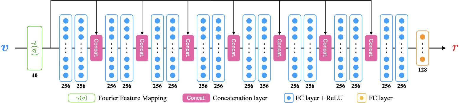
{\mathcal{M}}_{\phi}:{\bm{v}}\rightarrow r\quad\text{with}\quad{\bm{v}}\in\mathbb{R}^{v},\;r\in\mathbb{R},

where ${\bm{v}}$ represents the coordinate in the given imaging system, and $r$ is the corresponding sensor response. The network can be conceptually separated into two parts, where the first part is a single Fourier feature mapping (FFM) layer $\gamma({\bm{v}})$ that is pre-defined before training, while the second part is a standard MLP ${\mathcal{N}}_{\phi}:\gamma({\bm{v}})\rightarrow r$ whose parameters $\phi$ needs to be optimized. A visual illustration of the complete network architecture is provided in Figure 3. While the numerical studies presented in this paper focus on CT, CoIL is also applicable to other imaging modalities by simply changing the coordinate-response pairs in the MLP representation. For example, one can potentially integrate CoIL into optical diffraction tomography (ODT) [88, 89, 90] by letting ${\bm{v}}$ denote the sensor location and the angle of the incident light and letting $r$ have two elements corresponding to the real and imaginary components of the light-field.

3.1.1 Fourier feature mapping

Although neural networks are known to be universal function approximators [91], it has been found that standard MLPs perform poorly in representing high-frequency variations [92, 37]. In our experiments, we also experienced such issues when we directly applied ${\mathcal{N}}_{\phi}$ to learning the mapping ${\bm{v}}\rightarrow r$ (see No FFM in Figure 5). In order to overcome the limitations of standard MLPs, we include the FFM layer to expand the input coordinate ${\bm{v}}$ as a combination of different frequency components

\displaystyle\gamma({\bm{v}})=\begin{pmatrix}{\textit{sin}}\left(k_{1}\pi{\bm{v}}\right),{\textit{cos}}\left(k_{1}\pi{\bm{v}}\right),\\ \vdots\\ {\textit{sin}}\left(k_{L}\pi{\bm{v}}\right),{\textit{cos}}\left(k_{L}\pi{\bm{v}}\right)\end{pmatrix},

(9)

where ${\textit{sin}}(\cdot)$ and ${\textit{cos}}(\cdot)$ compute element-wise sinusoidal and cosinusoidal values, respectively, and $\{k_{i}\}_{i=1}^{L}$ determine the frequencies in the mapping. The FFM layer pre-defines the frequency components so that the network ${\mathcal{N}}_{\phi}$ can actively select the ones that are the most useful for encoding sensor responses by learning the weights in the first layer. By manipulating the coefficients $k_{i}$ and total number of components $L>0$ , we can explicitly control the expanded spectrum and thus impose some implicit regularization. The FFM layer was first introduced in NeRF as positional encoding of spatial coordinates [37], and a follow-up work [83] has further explored its functionality by using a concept known as neural target kernels [93]. The original formulation of $\gamma({\bm{v}})$ in [37] sets $k_{i}$ as an exponential function $k_{i}=2^{i-1}$ with $L=10$ . We discovered that the presence of very high-frequency components leads to the overfitting of the MLP to the noise in the measurements. We thus adopted a linear sampling $k_{i}=\pi i/2$ in the Fourier space that leads to a higher number of frequency components in the low-frequency regions. Our empirical results show that our strategy can effectively improve ${\mathcal{M}}_{\phi}$ in representing high-frequency variations and preventing overfitting to noise (see Figure 5 for examples).

3.1.2 MLP Architecture

The network implementing ${\mathcal{N}}_{\phi}$ is composed of $17$ fully-connected (FC) layers. The first $16$ layers have $256$ hidden neurons whose outputs are activated by the rectified linear unit (ReLU), while the last layer has $128$ hidden neurons without any activation. We implement $7$ skip connections after every even-numbered (less than $16$ ) FC layer to concatenate the original input of ${\mathcal{N}}_{\phi}$ with the intermediate outputs. The use of skip connections in MLP has been shown to be beneficial for fast training [84] and better accuracy [85]. Note that although ${\mathcal{M}}_{\phi}$ is a fully connected network, its input corresponds to a single coordinate, which enables element-wise processing of all the measurements.

3.1.3 Additional implementation details

CoIL trains a separate MLP to represent the full measurement field for each test objects. This means that the training pairs $\{({\bm{v}}_{i},r_{i})\}_{i=1}^{N}$ are obtained by extracting the measurements of the test object only, without any training dataset. The network ${\mathcal{M}}_{\phi}$ is trained by using Adam [94] to minimize the standard $\ell_{2}$ -norm loss

\ell(\psi)=\frac{1}{N}\sum_{i=1}^{N}\|{\mathcal{M}}_{\phi}({\bm{v}}_{i})-r_{i}\|_{2}^{2}.

(10)

We implement a decreasing learning rate, which decays exponentially as the training epoch increases, to smooth our optimization. Although ${\mathcal{M}}_{\phi}$ is a MLP, the network has a significantly smaller size ( $\approx 13$ MB on disk) compared to the standard UNet architecture ( $\approx 108$ MB on disk) used in many DL-based models.

3.2 Image reconstruction in CoIL

After training, one can generate an arbitrary number of measurements by querying ${\mathcal{M}}_{\phi}$ using the relevant coordinates. We will refer to the corresponding measurement field as CoIL field. The CoIL field can be readily integrated into the majority of image reconstruction methods. Here, we discuss the integration of CoIL into four widely-used methods.

3.2.1 Linear reconstruction

Filtered backprojection (FBP) is a classic method for bringing the measurements into the image domain [95]. Since the CoIL field is essentially a set of measurements, we can directly feed the field as input to FBP for image reconstruction. A slightly different way to apply FBP is to form a combined input that includes both the original measurements and those generated by CoIL. The key benefit of the latter approach is that it directly uses the real data while also complementing it with CoIL measurements.

3.2.2 Model-based optimization

Model-based methods reconstruct images by solving optimization problems of form (2). The CoIL field can be incorporated into the formulation by including an additional “data-fidelity” term $\tilde{g}$ in the objective

f({\bm{x}})=\underbrace{(1-\alpha)g({\bm{x}})+\alpha\tilde{g}({\bm{x}})}_{\text{New data-fidelity}}+h({\bm{x}}).

(11)

Here, the parameter $0\leq\alpha\leq 1$ controls the tradeoff between the real data and the generated field. In practice, we can fine-tune the value of $\alpha$ to obtain a good balance between two terms. For example, consider the least-squares function

\tilde{g}({\bm{x}})=\frac{1}{2}\|\tilde{{\bm{A}}}{\bm{x}}-{\mathcal{M}}_{\phi}(\tilde{{\bm{v}}})\|_{2}^{2},

(12)

where $\tilde{{\bm{A}}}\in\mathbb{R}^{m\times n}$ corresponds to the sampling geometry of the CoIL field, $\tilde{{\bm{v}}}$ represents all the query coordinates for the trained MLP ${\mathcal{M}}_{\phi}(\tilde{{\bm{v}}})$ . Since the network is pre-trained, one can directly use any existing image regularizer and solve the optimization problem with a standard iterative algorithm, such as FISTA or ADMM.

Table 1: The average SNR of the sinograms generated by No FFM, Pos Enc, and CoIL in the scenarios corresponding to

P\times I=\{60,90,120\}\times\{30,40,50\}

# Views	Noise Level	MLP Architectures
( $P$ )	( $I$ )	No FFM	Pos Enc	CoIL

$60$	$30$	$33.95$	$15.25$	$\mathbf{37.34}$
	$40$	$42.62$	$21.79$	$\mathbf{43.68}$
	$50$	$46.33$	$23.92$	$\mathbf{48.41}$

$90$	$30$	$34.93$	$23.68$	$\mathbf{38.56}$
	$40$	$43.82$	$30.56$	$\mathbf{44.72}$
	$50$	$48.08$	$35.34$	$\mathbf{50.50}$

$120$	$30$	$36.24$	$22.91$	$\mathbf{39.34}$
	$40$	$44.81$	$24.37$	$\mathbf{45.29}$
	$50$	$49.68$	$26.52$	$\mathbf{51.59}$

3.2.3 End-to-end DL models

As reviewed in Section 2.2, most end-to-end DL models are trained to directly map the low-quality images $\{{\tilde{{\bm{x}}}}_{i}\}_{i=1}^{N}$ to the high-quality images $\{{\bm{x}}_{i}\}_{i=1}^{N}$ , making them vulnerable to unseen outliers. For example, this adversely influences the performance of DL, when there is a mismatch between training and testing angles. CoIL can be used to address this issue by generating the measurement field corresponding to the same subsampling rate as the measurements used for training the DL model

{\widehat{\bm{x}}}={\mathcal{F}}_{\psi}(\text{FBP}({\mathcal{M}}_{\phi}(\tilde{{\bm{v}}}))),

(13)

where ${\mathcal{F}}_{\psi}$ denotes the pre-trained CNN. Alternatively, one can include the original test image in the input by averaging the ${\tilde{{\bm{x}}}}$ and $\text{FBP}({\mathcal{M}}_{\phi}(\tilde{{\bm{v}}}))$ using a weight $\alpha$

{\widehat{\bm{x}}}={\mathcal{F}}_{\psi}(\underbrace{(1-\alpha){\tilde{{\bm{x}}}}+\alpha\text{FBP}({\mathcal{M}}_{\phi}(\tilde{{\bm{v}}}))}_{\text{Joint input}}).

(14)

This approach enables the usage of the learned measurements by MLP with the true measurements from the imaging system. Our results in Section 4 show that this CoIL-based strategy achieves better results than training a DL model directly on the measurements.

3.2.4 Denoising-driven approches

Table 2: The average SNR values obtained with and without CoIL by using FBP, FISTA-TV, GM-RED, and FBP-UNet in the scenarios corresponding to

P\times I=\{60,90,120\}\times\{30,40,50\}

# Views	Noise Level	without CoIL				with CoIL
( $P$ )	( $I$ )	FBP	FISTA-TV	GM-RED	FBP-UNet	FBP	FISTA-TV	GM-RED	FBP-UNet

$60$	$30$	$0.15$	$22.66$	22.77	$23.44$	$\mathbf{19.45}$	$\mathbf{22.81}$	$\mathbf{23.01}$	$\mathbf{24.17}$
	$40$	$9.09$	$26.08$	$27.12$	$27.08$	$\mathbf{23.48}$	$\mathbf{26.95}$	$\mathbf{27.42}$	$\mathbf{27.93}$
	$50$	$14.25$	$29.37$	$30.75$	$29.52$	$\mathbf{24.99}$	$\mathbf{29.78}$	$\mathbf{30.88}$	$\mathbf{30.54}$

$90$	$30$	$1.95$	$23.32$	$23.37$	$24.43$	$\mathbf{20.15}$	$\mathbf{23.58}$	$\mathbf{23.64}$	$\mathbf{25.20}$
	$40$	$10.92$	$26.98$	$28.86$	$28.57$	$\mathbf{24.14}$	$\mathbf{28.28}$	$\mathbf{29.31}$	$\mathbf{29.28}$
	$50$	$16.07$	$30.76$	$31.71$	$31.84$	$\mathbf{25.69}$	$\mathbf{31.78}$	$\mathbf{32.19}$	$\mathbf{32.23}$

$120$	$30$	$3.21$	$23.79$	$24.00$	$24.68$	$\mathbf{20.63}$	$\mathbf{24.08}$	$\mathbf{24.39}$	$\mathbf{25.62}$
	$40$	$12.10$	$27.59$	$29.30$	$29.18$	$\mathbf{24.52}$	$\mathbf{28.95}$	$\mathbf{29.79}$	$\mathbf{29.71}$
	$50$	$17.07$	$31.53$	$32.31$	$32.80$	$\mathbf{26.02}$	$\mathbf{32.89}$	$\mathbf{33.02}$	$\mathbf{33.31}$

PnP/RED algorithms can be interpreted as extensions of model-based algorithms balancing consistency with the measurements against deep denoising priors [25, 22]. Consider gradient-based RED (GM-RED)

{\bm{x}}^{+}\leftarrow{\bm{x}}-\gamma\left[\nabla g({\bm{x}})+\tau({\bm{x}}-{\mathcal{D}}_{\sigma}({\bm{x}}))\right]

(15)

where $\gamma>0$ is the stepsize, and $\nabla g$ is the gradient of the data-fidelity term. Similar to the modification of model-based optimization, one straightforward way to integrate CoIL into GM-RED is to include the gradient of $\tilde{g}$ as an extra term

{\bm{x}}^{+}\leftarrow{\bm{x}}-\gamma[\underbrace{(1-\alpha)\nabla g({\bm{x}})+\alpha\nabla\tilde{g}({\bm{x}})}_{\text{New data enforcement}}+\tau({\bm{x}}-{\mathcal{D}}_{\sigma}({\bm{x}}))],

where the new update ensures the consistency with the real measurements as well as the field generated by CoIL, with $\alpha$ controlling the relative weighting. This idea is also applicable to PnP, for example, by integrating CoIL within PnP-FISTA


$\displaystyle{\bm{x}}^{+}$	$\displaystyle\leftarrow{\mathcal{D}}_{\sigma}({\bm{s}}-\gamma[(1-\alpha)\nabla g({\bm{s}})+\alpha\nabla\tilde{g}({\bm{s}})])$	(16a)
$\displaystyle{\bm{s}}^{+}$	$\displaystyle\leftarrow{\bm{x}}^{+}+((q^{+}-1)/q^{+})({\bm{x}}^{+}-{\bm{x}})$	(16b)

where the acceleration parameter $q>0$ is updated as

q^{+}\leftarrow\frac{1}{2}\left(1+\sqrt{1+4q^{2}}\right).

In the next section, we will provide results highlighting the performance of CoIL in the context of all these algorithms.

4 Numerical Validations

We numerically validate CoIL in the context of sparse-view CT. We first substantiate the effectiveness of the proposed form of FFM, and then demonstrate the benefits of using CoIL for image reconstruction. We consider four reconstruction methods, FBP, FISTA-TV, GM-RED, and FBP-UNet. FBP-UNet refers to the end-to-end model proposed in [9] and FISTA-TV refers to the TV regularized inversion implemented using FISTA. We integrate CoIL into these algorithm by including the parameter $\alpha$ as discussed in Section 3.2.

4.1 Sparse view CT and experimental setup

Sparse view X-ray CT is an imaging modality that aims to reconstruct a tomographic image from few projections. In medical applications, it can significantly reduce the radiation dose and hence reduce the risk of radiation exposure. The reconstruction task in CT can be formulated as the linear inverse problem of form (1). In our simulations, we adopt the parallel beam geometry with a measurement operator ${\bm{A}}$ corresponding to the Radon transform.

We consider the experimental setting where the X-ray beam is emitted from the view angle $\theta\in[0,\pi]$ and its radiation attenuation is recorded by the detectors at different (normalized) sensor-plane locations $l\in[0,1]$ . Thus, the MLP is trained to map the location and angle $(l,\theta)$ to the corresponding response $r$ . Figure 4 visualizes eight $512\times 512$ test images used in all experiments. These images are selected from the scans of two patients in the APPM human phantom dataset¹¹ 1 The 2016 NIH-AAPM-Mayo Clinic Low Dose CT Grand Challenge [96], while the scans of other patients are used for training the FBP-UNet and the deep denoiser in GM-RED. We implemented ${\bm{A}}$ and its adjoint ${\bm{A}}^{{\mathsf{T}}}$ by using RayTransform from the Operator Discretization Library (ODL) [97], which allows fast computation using a GPU backend. We synthesized the test sinograms corresponding to $P\in\{60,90,120\}$ projection views, each further contaminated by three noise levels equivalent to the input signal-to-noise ratio (SNR) of $I\in\{30,40,50\}$ dB. SNR is also used as a metric to quantify the reconstruction quality

\displaystyle\operatorname{SNR}(\hat{{\bm{x}}},{\bm{x}})\triangleq 20\operatorname{log}_{10}\left(\frac{\|{\bm{x}}\|_{2}}{\|{\bm{x}}-\hat{{\bm{x}}}\|_{2}}\right).

(17)

We denote the SNR values averaged over all test images as average SNR.

For each test image, CoIL trains separate MLPs to represent its full measurement field in different scenarios $P\times I=\{60,90,120\}\times\{30,40,50\}$ . We conducted all the experiments, as well as the training of all neural networks, on a machine equipped with an Intel Xeon Gold 6130 Processor and four Nvidia GeForce GTX 1080 Ti GPUs. The training time of a single MLP on our machine takes about $30$ minutes.

4.2 Effectiveness of the FFM layer

We first evaluate the effectiveness of the proposed FFM layer used in the coordinate-based MLP. We trained and compared three networks where: (a) the FFM layer is not implemented (No FFM); (b) the FFM layer implements the positional encoding where $k_{i}=2^{k-i}$ (Pos Enc); and (c) the FFM layer implements the proposed linear expansion $k_{i}=(\pi i)/2$ (CoIL). In the simulations, we use these networks to generate the sinograms corresponding to $360$ views, and the total number of frequency components is set to $L=10$ for both Pos Enc and CoIL.

Table 1 summarizes the average SNR values of the sinograms generated by the three networks in all scenarios. Here, we use SNR as the quality metric in the sinogram space, because it enables straightforward comparison with the original measurements whose noise level is characterized by input SNR. As shown in the table, CoIL consistently achieves significantly higher SNR values than both No FFM and Pos Enc. Our interpretation is that No FFM is unable to represent the high-frequency variations in the measurement field, while Pos Enc overfits to noise by containing too many high-frequency components. We observe that the sampling pattern in CoIL better captures the nature of the measurements without overfitting to the noise. This is further illustrated in visual examples in Figure 5, which plots the sinograms and their FBP reconstructions obtained by each network for $P=120$ and $I=40$ dB. Specifically, No FFM is able to represent the general structure of the sinogram but fails in generating the details; Pos Enc produces strong artifacts in its sinogram due to its FFM layer. CoIL succeeds in both representing the high-frequency details and avoiding strong artifacts in the generated measurements. The improvement in the sinogram quality is also reflected in the SNR values obtained after FBP reconstruction. Note how CoIL significantly differs from other approaches in the regions highlighted by the bounding boxes.

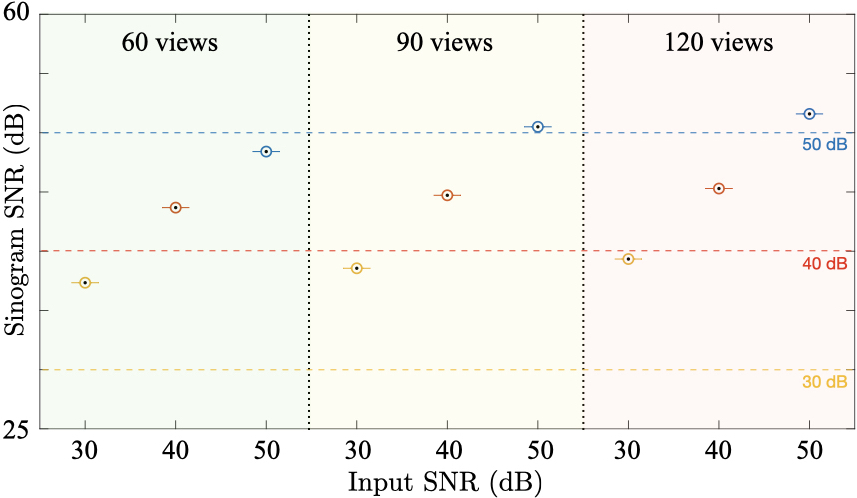
We have also investigated the evolution of the sinogram quality for different number of views and noise levels. Figure 5 plots the SNR of the sinograms obtained by CoIL against the input SNR ( $I\in\{30,40,50\}$ ) for different number of views ( $P\in\{60,90,120\}$ ). The three dotted horizontal lines in the figure highlight each $I$ value. We first note that CoIL generates sinograms that generally have higher SNR than the noise level in the measurements. In particular, when $I=30$ dB, the average SNR values are more than $7$ dB higher for every $P$ . This highlights the ability of CoIL to generate high-quality sinograms. The figure also demonstrates that the SNR values improve as the number of views increases or noise level decreases. This highlights that the quality of the CoIL fields can be improved by having more measurements or acquiring those that are less noisy.

4.3 Performance evaluation of CoIL

We next highlight the benefit of CoIL for image reconstruction. We trained all our MLPs by using the FFM layer based on our linear expansion. We implemented FBP by using fbp-op from the ODL package under the default parameter setting. We used DnCNN [46] to build the deep denoiser within GM-RED. In every experiment, we selected the network achieving the highest SNR value from the ones corresponding to five noise levels $\sigma\in\{5,10,15,20,25\}$ . For FBP, FISTA-TV, and GM-RED, CoIL generates the measurement field with $360$ projection views from the test measurements. For FBP-UNet using CoIL, we trained the CNN on the dataset consisting of the measurements having $1.5\times P=\{90,135,180\}$ projection views and used CoIL to generate additional measurements to achieve that number. As a baseline, we trained a separate FBP-UNet that directly predicts the groundtruth form the test measurements. Note that the baseline networks correspond to the optimal performance that FBP-UNet can achieve for the test measurements without integrating CoIL. In order to stabilize FBP-UNet, we trained these networks using the data with random fluctuations in both projection views ( $\pm 15$ ) and noise amount ( $\pm 5$ dB).

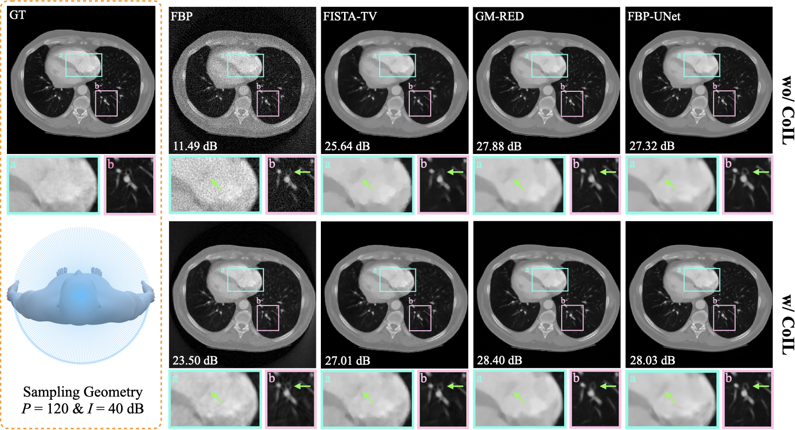
Figure 7 quantitatively evaluates the improvements in imaging quality due to CoIL for all the considered reconstruction algorithms. For each algorithm, we plot the difference between the SNR obtained with and without CoIL. We can clearly observe that CoIL leads to significant quality improvements for all the algorithms. Remarkably, for the higher amount of noise ( $I=30$ dB), the average improvement by CoIL can sometimes be as high as $20$ dB for FBP. On the other hand, when the noise is relatively mild, CoIL still leads to significant SNR improvements for all algorithms including model-based and DL-based methods. In particular, for $P=60$ and $I=50$ dB, FBP-UNet without CoIL achieves $29.52$ dB, while FBP-UNet with CoIL achieves $30.54$ dB, which is nearly $1$ dB improvement. The exact numbers obtained by each algorithm are also summarized in Table 2. These results highlight that CoIL is able to accurately represent the measurement field and generate high-fidelity measurements that can be used to improve image reconstruction.

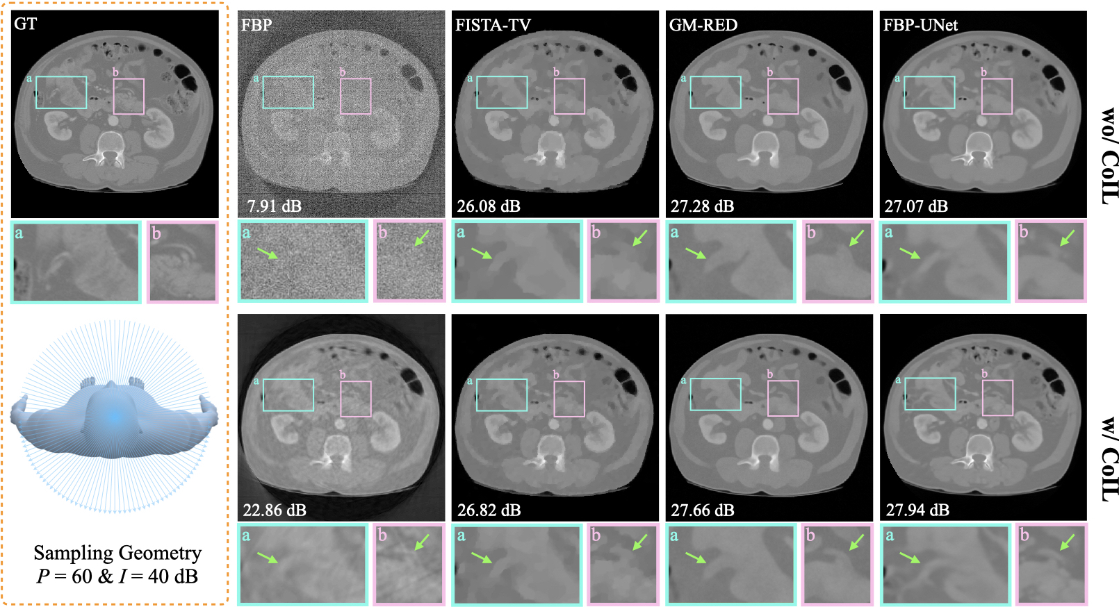
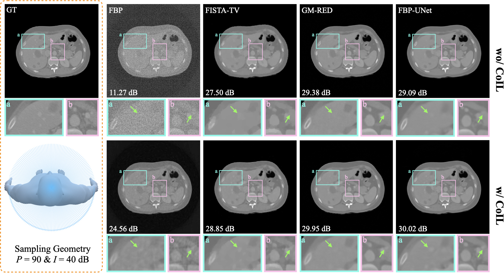
Figure 8 presents visual comparisons of images reconstructed with and without CoIL for $P=60$ and $I=40$ . Each image is labeled with its SNR with respect to the groundtruth and the visual differences are highlighted by arrows in the bounding boxes. This comparison highlights visual improvements due to CoIL. For example, consider the visual differences for FBP-Unet, where one can clearly see additional visual details after integration of the CoIL field. The better reconstruction quality with CoIL is also reflected in the higher SNR values. Additional visual comparisons in Figure 9 and Figure 10 also highlight the benefit of image reconstruction with CoIL.

5 Conclusion

The CoIL methodology developed in this paper is a new approach for computational imaging using coordinate-based neural representations. CoIL can represent the full measurement field as a single MLP network by training it to map the measurement coordinates to their sensor responses. This makes CoIL a self-supervised model that can be trained without any external dataset. We provided extensive empirical results demonstrating the improvements due to CoIL in the context of sparse-view CT, highlighting its great potential to work synergistically with existing image reconstruction methods. Future work will explore new applications of CoIL to other imaging modalities, such as optical diffraction tomography and intensity diffraction tomography.

Acknowledgement

The research in this work was supported by NSF award CCF-1813910 and by the Laboratory Directed Research and Development program of Los Alamos National Laboratory under project number 20200061DR.

References

[1] L. I. Rudin, S. Osher, and E. Fatemi, “Nonlinear total variation based noise removal algorithms,” Physica D, vol. 60, no. 1–4, pp. 259–268, Nov. 1992.
[2] M. A. T. Figueiredo and R. D. Nowak, “Wavelet-based image estimation: An empirical Bayes approach using Jeffreys’ noninformative prior,” IEEE Trans. Image Process., vol. 10, no. 9, pp. 1322–1331, Sep. 2001.
[3] M. Elad and M. Aharon, “Image denoising via sparse and redundant representations over learned dictionaries,” IEEE Trans. Image Process., vol. 15, no. 12, pp. 3736–3745, Dec. 2006.
[4] A. Danielyan, V. Katkovnik, and K. Egiazarian, “BM3D frames and variational image deblurring,” IEEE Trans. Image Process., vol. 21, no. 4, pp. 1715–1728, Apr. 2012.
[5] M. T. McCann, K. H. Jin, and M. Unser, “Convolutional neural networks for inverse problems in imaging: A review,” IEEE Signal Process. Mag., vol. 34, no. 6, pp. 85–95, 2017.
[6] A. Lucas, M. Iliadis, R. Molina, and A. K. Katsaggelos, “Using deep neural networks for inverse problems in imaging: Beyond analytical methods,” IEEE Signal Process. Mag., vol. 35, no. 1, pp. 20–36, Jan. 2018.
[7] G. Ongie, A. Jalal, C. A. Metzler, R. G. Baraniuk, A. G. Dimakis, and R. Willett, “Deep learning techniques for inverse problems in imaging,” IEEE J. Sel. Areas Inf. Theory, vol. 1, no. 1, pp. 39–56, May 2020.
[8] G. Wang, J. C. Ye, and B. De Man, “Deep learning for tomographic image reconstruction,” Nature Machine Intelligence, vol. 2, no. 12, pp. 737–748, 2020.
[9] K. H. Jin, M. T. McCann, E. Froustey, and M. Unser, “Deep convolutional neural network for inverse problems in imaging,” IEEE Trans. Image Process., vol. 26, no. 9, pp. 4509–4522, Sep. 2017.
[10] E. Kang, J. Min, and J. C. Ye, “A deep convolutional neural network using directional wavelets for low-dose x-ray CT reconstruction,” Medical Physics, vol. 44, no. 10, pp. e360–e375, 2017.
[11] Y. Sun, Z. Xia, and U. S. Kamilov, “Efficient and accurate inversion of multiple scattering with deep learning,” Opt. Express, vol. 26, no. 11, pp. 14678–14688, May 2018.
[12] Y. Han and J. C. Ye, “Framing U-Net via deep convolutional framelets: Application to sparse-view CT,” IEEE Trans. Med. Imag., vol. 37, no. 6, pp. 1418–1429, 2018.
[13] S. V. Venkatakrishnan, C. A. Bouman, and B. Wohlberg, “Plug-and-play priors for model based reconstruction,” in Proc. IEEE Global Conf. Signal Process. and Inf. Process. (GlobalSIP), Austin, TX, USA, Dec. 3-5, 2013, pp. 945–948.
[14] Y. Romano, M. Elad, and P. Milanfar, “The little engine that could: Regularization by denoising (RED),” SIAM J. Imaging Sci., vol. 10, no. 4, pp. 1804–1844, 2017.
[15] S. Ono, “Primal-dual plug-and-play image restoration,” IEEE Signal. Proc. Let., vol. 24, no. 8, pp. 1108–1112, Aug. 2017.
[16] U. S. Kamilov, H. Mansour, and B. Wohlberg, “A plug-and-play priors approach for solving nonlinear imaging inverse problems,” IEEE Signal. Proc. Let., vol. 24, no. 12, pp. 1872–1876, Dec. 2017.
[17] S. A. Bigdeli, M. Zwicker, P. Favaro, and M. Jin, “Deep mean-shift priors for image restoration,” in Advances in Neural Information Processing Systems 30, 2017, pp. 763–772.
[18] Z. Wu, Y. Sun, A. Matlock, J. Liu, L. Tian, and U. S. Kamilov, “SIMBA: Scalable inversion in optical tomography using deep denoising priors,” IEEE J. Sel. Topics Signal Process., pp. 1–1, 2020.
[19] J. Liu, Y. Sun, C. Eldeniz, W. Gan, H. An, and U. S. Kamilov, “RARE: Image reconstruction using deep priors learned without ground truth,” IEEE J. Sel. Topics Signal Process., pp. 1–1, 2020.
[20] S. H. Chan, X. Wang, and O. A. Elgendy, “Plug-and-play ADMM for image restoration: Fixed-point convergence and applications,” IEEE Trans. Comp. Imag., vol. 3, no. 1, pp. 84–98, Mar. 2017.
[21] G. T. Buzzard, S. H. Chan, S. Sreehari, and C. A. Bouman, “Plug-and-play unplugged: Optimization free reconstruction using consensus equilibrium,” SIAM J. Imaging Sci., vol. 11, no. 3, pp. 2001–2020, Sep. 2018.
[22] E. K. Ryu, J. Liu, S. Wang, X. Chen, Z. Wang, and W. Yin, “Plug-and-play methods provably converge with properly trained denoisers,” in Proc. 36th Int. Conf. Machine Learning (ICML), Long Beach, CA, USA, June 09–15 2019, vol. 97, pp. 5546–5557.
[23] Y. Sun, B. Wohlberg, and U. S. Kamilov, “An online plug-and-play algorithm for regularized image reconstruction,” IEEE Trans. Comput. Imaging, vol. 5, no. 3, pp. 395–408, Sept. 2019.
[24] X. Xu, Y. Sun, J. Liu, B. Wohlberg, and U. S. Kamilov, “Provable convergence of plug-and-play priors with mmse denoisers,” IEEE Signal Process. Lett., vol. 27, pp. 1280–1284, 2020.
[25] Y. Sun, J. Liu, and U. S. Kamilov, “Block coordinate regularization by denoising,” in Advances in Neural Information Processing Systems 32, pp. 380–390. 2019.
[26] J. Zhang and B. Ghanem, “ISTA-Net: Interpretable optimization-inspired deep network for image compressive sensing,” in Proc. IEEE Conf. Comput. Vision Pattern Recognit., 2018, pp. 1828–1837.
[27] Y. Yang, J. Sun, H. Li, and Z. Xu, “Deep ADMM-Net for compressive sensing MRI,” in Advances in Neural Information Processing Systems 29, 2016, pp. 10–18.
[28] A. Hauptmann, F. Lucka, M. Betcke, N. Huynh, J. Adler, B. Cox, P. Beard, S. Ourselin, and S. Arridge, “Model-based learning for accelerated, limited-view 3-d photoacoustic tomography,” IEEE Trans. Med. Imag., vol. 37, no. 6, pp. 1382–1393, 2018.
[29] J. Adler and O. Öktem, “Learned primal-dual reconstruction,” IEEE Trans. Med. Imag., vol. 37, no. 6, pp. 1322–1332, June 2018.
[30] H. K. Aggarwal, M. P. Mani, and M. Jacob, “MoDL: Model-based deep learning architecture for inverse problems,” IEEE Trans. Med. Imag., vol. 38, no. 2, pp. 394–405, Feb. 2019.
[31] S. A. Hosseini, B. Yaman, S. Moeller, M. Hong, and M. Akcakaya, “Dense recurrent neural networks for accelerated MRI: History-cognizant unrolling of optimization algorithms,” IEEE J. Sel. Topics Signal Process., vol. 14, no. 6, pp. 1280–1291, Oct. 2020.
[32] I. Y. Chun, Z. Huang, H. Lim, and J. Fessler, “Momentum-Net: Fast and convergent iterative neural network for inverse problems,” IEEE Trans. Patt. Anal. and Machine Intell., pp. 1–1, 2020.
[33] B. Yaman, S. A. H. Hosseini, S. Moeller, J. Ellermann, K. Uğurbil, and M. Akçakaya, “Self-supervised learning of physics-guided reconstruction neural networks without fully sampled reference data,” Magn. Reson. Med., Jul. 2020.
[34] H. K. Aggarwal and M. Jacob, “J-MoDL: Joint model-based deep learning for optimized sampling and reconstruction,” IEEE J. Sel. Topics Signal Process., vol. 14, no. 6, pp. 1151–1162, 2020.
[35] M. Kellman, K. Zhang, E. Markley, J. Tamir, E. Bostan, M. Lustig, and L. Waller, “Memory-efficient learning for large-scale computational imaging,” IEEE Trans. Comput. Imag., vol. 6, pp. 1403–1414, 2020.
[36] J. Liu, Y. Sun, W. Gan, X. Xu, B. Wohlberg, and U. S. Kamilov, “SGD-Net: Efficient model-based deep learning with theoretical guarantees,” arXiv:2101.09379 [eess.IV], 2021.
[37] B. Mildenhall, P. P. Srinivasan, M. Tancik, J. T. Barron, R. Ramamoorthi, and R. Ng, “NeRF: Representing scenes as neural radiance fields for view synthesis,” in The European Conference on Computer Vision (ECCV), 2020.
[38] R. Martin-Brualla, N. Radwan, M. SM Sajjadi, J. T Barron, A. Dosovitskiy, and D. Duckworth, “NeRF in the wild: Neural radiance fields for unconstrained photo collections,” arXiv:2008.02268 [cs.CV], 2020.
[39] K. Zhang, G. Riegler, N. Snavely, and V. Koltun, “NeRF++: Analyzing and improving neural radiance fields,” arXiv:2010.07492 [cs.CV], 2020.
[40] A. Beck and M. Teboulle, “A fast iterative shrinkage-thresholding algorithm for linear inverse problems,” SIAM J. Imaging Sci., vol. 2, no. 1, pp. 183–202, 2009.
[41] S. Boyd, N. Parikh, E. Chu, B. Peleato, and J. Eckstein, “Distributed optimization and statistical learning via the alternating direction method of multipliers,” Foundations and Trends in Machine Learning, vol. 3, no. 1, pp. 1–122, July 2011.
[42] J. J. Moreau, “Proximité et dualité dans un espace Hilbertien,” Bull. Soc. Math. France, vol. 93, pp. 273–299, 1965.
[43] O. Ronneberger, P. Fischer, and T. Brox, “U-Net: Convolutional networks for biomedical image segmentation,” in Medical Image Computing and Computer-Assisted Intervention (MICCAI), Munich, Germany, Oct. 5-9 2015, pp. 234–241.
[44] T. Würfl, M. Hoffmann, V. Christlein, K. Breininger, Y. Huang, M. Unberath, and A. K. Maier, “Deep learning computed tomography: Learning projection-domain weights from image domain in limited angle problems,” IEEE Trans. on Med. Imag., vol. 37, no. 6, pp. 1454–1463, 2018.
[45] B. Zhu, J. Z Liu, S. F Cauley, B. R Rosen, and M. S Rosen, “Image reconstruction by domain-transform manifold learning,” Nature, vol. 555, no. 7697, pp. 487–492, 2018.
[46] K. Zhang, W. Zuo, Y. Chen, D. Meng, and L. Zhang, “Beyond a Gaussian denoiser: Residual learning of deep CNN for image denoising,” IEEE Trans. Image Process., vol. 26, no. 7, pp. 3142–3155, July 2017.
[47] K. Zhang, W. Zuo, and L. Zhang, “FFDNet: Toward a fast and flexible solution for CNN-based image denoising,” IEEE Trans. Image Process., vol. 27, no. 9, pp. 4608–4622, Sep. 2018.
[48] G. Song, Y. Sun, J. Liu, Z. Wang, and U. S. Kamilov, “A new recurrent plug-and-play prior based on the multiple self-similarity network,” IEEE Signal Process. Lett., vol. 27, no. 1, pp. 451–455, 2020.
[49] S. Sreehari, S. V. Venkatakrishnan, B. Wohlberg, G. T. Buzzard, L. F. Drummy, J. P. Simmons, and C. A. Bouman, “Plug-and-play priors for bright field electron tomography and sparse interpolation,” IEEE Trans. Comput. Imaging, vol. 2, no. 4, pp. 408–423, Dec. 2016.
[50] K. Zhang, W. Zuo, S. Gu, and L. Zhang, “Learning deep CNN denoiser prior for image restoration,” in Proc. IEEE Conf. Computer Vision and Pattern Recognition (CVPR), 2017, pp. 3929–3938.
[51] Y. Sun, S. Xu, Y. Li, L. Tian, B. Wohlberg, and U. S. Kamilov, “Regularized Fourier ptychography using an online plug-and-play algorithm,” in Proc. IEEE Int. Conf. Acoustics, Speech and Signal Process. (ICASSP), Brighton, UK, May 12-17, 2019, pp. 7665–7669.
[52] Kai Zhang, Wangmeng Zuo, and Lei Zhang, “Deep plug-and-play super-resolution for arbitrary blur kernels,” in Proceedings of the IEEE Conference on Computer Vision and Pattern Recognition (CVPR), 2019, pp. 1671–1681.
[53] R. Ahmad, C. A. Bouman, G. T. Buzzard, S. Chan, S. Liu, E. T. Reehorst, and P. Schniter, “Plug-and-play methods for magnetic resonance imaging: Using denoisers for image recovery,” IEEE Signal Processing Magazine, vol. 37, no. 1, pp. 105–116, 2020.
[54] T. Meinhardt, M. Moeller, C. Hazirbas, and D. Cremers, “Learning proximal operators: Using denoising networks for regularizing inverse imaging problems,” in Proc. IEEE Int. Conf. Comp. Vis. (ICCV), 2017, pp. 1799–1808.
[55] T. Tirer and R. Giryes, “Image restoration by iterative denoising and backward projections,” IEEE Trans. Image Process., vol. 28, no. 3, pp. 1220–1234, Mar. 2019.
[56] A. M. Teodoro, J. M. Bioucas-Dias, and M. A. T. Figueiredo, “A convergent image fusion algorithm using scene-adapted Gaussian-mixture-based denoising,” IEEE Trans. Image Process., vol. 28, no. 1, pp. 451–463, Jan. 2019.
[57] Yu Sun, Jiaming Liu, Yiran Sun, Brendt Wohlberg, and Ulugbek Kamilov, “Async-RED: A provably convergent asynchronous block parallel stochastic method using deep denoising priors,” in International Conference on Learning Representations (ICLR), 2021.
[58] Gary Mataev, Peyman Milanfar, and Michael Elad, “DeepRED: Deep image prior powered by RED,” in The IEEE International Conference on Computer Vision (ICCV) Workshops, Oct. 2019.
[59] C. Metzler, P. Schniter, A. Veeraraghavan, and R. Baraniuk, “prDeep: Robust phase retrieval with a flexible deep network,” in Proc. 35th Int. Conf. Machine Learning (ICML), Stockholmsmässan, Stockholm Sweden, 10–15 July 2018, pp. 3501–3510.
[60] E. T. Reehorst and P. Schniter, “Regularization by denoising: Clarifications and new interpretations,” IEEE Trans. Comput. Imag., vol. 5, no. 1, pp. 52–67, Mar. 2019.
[61] R. Cohen, M. Elad, and P. Milanfar, “Regularization by denoising via fixed-point projection (RED-PRO),” arXiv:2008.00226 [eess.IV], 2020.
[62] K. Gregor and Y. LeCun, “Learning fast approximation of sparse coding,” in Proc. 27th Int. Conf. Machine Learning (ICML), Haifa, Israel, June 21-24, 2010, pp. 399–406.
[63] S. Biswas, H. K. Aggarwal, and M. Jacob, “Dynamic MRI using model‐based deep learning and SToRM priors: MoDL‐SToRM,” Magn. Reson. Med., vol. 82, no. 1, pp. 485–494, July 2019.
[64] A. Bora, A. Jalal, E. Price, and A. G. Dimakis, “Compressed sensing using generative models,” in Proc. 34th Int. Conf. Machine Learning (ICML), International Convention Centre, Sydney, Australia, 06–11 Aug 2017, vol. 70, pp. 537–546.
[65] V. Shah and C. Hegde, “Solving linear inverse problems using gan priors: An algorithm with provable guarantees,” in 2018 IEEE international conference on acoustics, speech and signal processing (ICASSP). IEEE, 2018, pp. 4609–4613.
[66] A. Jalal, L. Liu, A. G Dimakis, and C. Caramanis, “Robust compressed sensing using generative models,” Advances in Neural Information Processing Systems, vol. 33, 2020.
[67] N. Shlezinger, J. Whang, Y. C Eldar, and A. G Dimakis, “Model-based deep learning,” arXiv:2012.08405 [eess.SP], 2020.
[68] H. Lee, J. Lee, and S. Cho, “View-interpolation of sparsely sampled sinogram using convolutional neural network,” in Medical Imaging 2017: Image Processing, Martin A. Styner and Elsa D. Angelini, Eds., 2017, vol. 10133, pp. 617 – 624.
[69] H. Lee, J. Lee, H. Kim, B. Cho, and S. Cho, “Deep-neural-network-based sinogram synthesis for sparse-view CT image reconstruction,” IEEE Transactions on Radiation and Plasma Medical Sciences, vol. 3, no. 2, pp. 109–119, 2019.
[70] R. Anirudh, H. Kim, J. J Thiagarajan, K Aditya Mohan, K. Champley, and T. Bremer, “Lose the views: Limited angle CT reconstruction via implicit sinogram completion,” in Proceedings of the IEEE Conference on Computer Vision and Pattern Recognition (CVPR), 2018, pp. 6343–6352.
[71] M. U. Ghani and W C. Karl, “Fast enhanced CT metal artifact reduction using data domain deep learning,” IEEE Trans. Comput. Imag., vol. 6, pp. 181–193, 2019.
[72] Muhammad Usman Ghani and W Clem Karl, “Data and image prior integration for image reconstruction using consensus equilibrium,” arXiv:2009.00092[eess.IV], 2020.
[73] M. U. Ghani, Data and image domain deep learning for computational imaging, Ph.D. thesis, 2021.
[74] B. EH Claus, Y. Jin, L. A Gjesteby, G. Wang, and B. De Man, “Metal-artifact reduction using deep-learning based sinogram completion: Initial results,” in Proc. 14th Int. Meeting Fully Three-Dimensional Image Reconstruction Radiology Nuclear Medicine, 2017, pp. 631–634.
[75] Q. De Man, E. Haneda, B. Claus, P. Fitzgerald, B. De Man, G. Qian, H. Shan, J. Min, M. Sabuncu, and G. Wang, “A two-dimensional feasibility study of deep learning-based feature detection and characterization directly from CT sinograms,” Medical physics, vol. 46, no. 12, pp. 790–800, 2019.
[76] Y. Han, L. Sunwoo, and J. C. Ye, “ ${k}$ -space deep learning for accelerated MRI,” IEEE Trans. Med. Imag., vol. 39, no. 2, pp. 377–386, 2020.
[77] Mehmet A., Steen M., Sebastian W., and Kâmil U., “Scan-specific robust artificial-neural-networks for k-space interpolation (RAKI) reconstruction: Database-free deep learning for fast imaging,” Magn. Reson. Med., vol. 81, no. 1, pp. 439–453, 2019.
[78] A. Shocher, N. Cohen, and M. Irani, “‘Zero-shot’ super-resolution using deep internal learning,” in Proceedings of the IEEE Conference on Computer Vision and Pattern Recognition (CVPR), 2018, pp. 3118–3126.
[79] L. P. Zuckerman, E. Naor, G. Pisha, S. Bagon, and M. Irani, “Across scales and across dimensions: Temporal super-resolution using deep internal learning,” in European Conference on Computer Vision (ECCV), 2020, pp. 52–68.
[80] D. Ulyanov, A. Vedaldi, and V. Lempitsky, “Deep image prior,” in Proc. IEEE Conf. Computer Vision and Pattern Recognition (CVPR), Salt Lake City, UT, USA, June 18-22, 2018, pp. 9446–9454.
[81] J. Liu, Y. Sun, X. Xu, and U. S. Kamilov, “Image restoration using total variation regularized deep image prior,” in 2019 IEEE International Conference on Acoustics, Speech and Signal Processing (ICASSP), May 2019, pp. 7715–7719.
[82] Y. Gandelsman, A. Shocher, and M. Irani, “‘Double-DIP’: Unsupervised image decomposition via coupled deep-image-priors,” in Proceedings of the IEEE/CVF Conference on Computer Vision and Pattern Recognition (CVPR), June 2019, pp. 11026–11035.
[83] M. Tancik, P. P. Srinivasan, B. Mildenhall, S. Fridovich-Keil, N. Raghavan, U. Singhal, R. Ramamoorthi, J. T. Barron, and R. Ng, “Fourier features let networks learn high frequency functions in low dimensional domains,” Advances in Neural Information Processing Systems 33, 2020.
[84] Z. Chen and H. Zhang, “Learning implicit fields for generative shape modeling,” in Proceedings of the IEEE Conference on Computer Vision and Pattern Recognition (CVPR), 2019, pp. 5939–5948.
[85] J. J. Park, P. Florence, J. Straub, Ri. Newcombe, and S. Lovegrove, “DeepSDF: Learning continuous signed distance functions for shape representation,” in Proceedings of the IEEE Conference on Computer Vision and Pattern Recognition (CVPR), 2019, pp. 165–174.
[86] P. P. Srinivasan, B. Deng, X. Zhang, M. Tancik, B. Mildenhall, and J. T. Barron, “NeRV: Neural reflectance and visibility fields for relighting and view synthesis,” in arXiv:2012.03927 [cs.CV], 2020.
[87] K. Park, U. Sinha, J. T Barron, S. Bouaziz, D. B Goldman, S. M Seitz, and R. Brualla, “Deformable neural radiance fields,” arXiv:2011.12948 [cs.CV], 2020.
[88] Y. Sung, W. Choi, C. Fang-Yen, K. Badizadegan, R. R. Dasari, and M. S. Feld, “Optical diffraction tomography for high resolution live cell imaging,” Opt. Express, vol. 17, no. 1, pp. 266–277, December 2009.
[89] U. S. Kamilov, I. N. Papadopoulos, M. H. Shoreh, A. Goy, C. Vonesch, M. Unser, and D. Psaltis, “Learning approach to optical tomography,” Optica, vol. 2, no. 6, pp. 517–522, June 2015.
[90] T.-A. Pham, E. Soubies, A. Goy, J. Lim, F. Soulez, D. Psaltis, and M. Unser, “Versatile reconstruction framework for diffraction tomography with intensity measurements and multiple scattering,” Opt Express, vol. 26, no. 3, pp. 2749–2763, February 2018.
[91] K. Hornik, M. Stinchcombe, H. White, et al., “Multilayer feedforward networks are universal approximators.,” Neural networks, vol. 2, no. 5, pp. 359–366, 1989.
[92] N. Rahaman, A. Baratin, D. Arpit, F. Draxler, M. Lin, F. Hamprecht, Y. Bengio, and A. Courville, “On the spectral bias of neural networks,” in International Conference on Machine Learning, 2019, pp. 5301–5310.
[93] A. Jacot, F. Gabriel, and C. Hongler, “Neural tangent kernel: Convergence and generalization in neural networks,” in Advances in neural information processing systems 31, 2018, pp. 8571–8580.
[94] D. Kingma and J. Ba, “Adam: A method for stochastic optimization,” in International Conference on Learning Representations (ICLR), 2015.
[95] A. C. Kak and M. Slaney, Principles of Computerized Tomographic Imaging, IEEE, 1988.
[96] C. McCollough, “TU-FG-207A-04: Overview of the low dose CT grand challenge,” Med. Phys, vol. 43, no. 6Part35, pp. 3759–3760, 2016.
[97] J. Adler and O. Öktem, “Solving ill-posed inverse problems using iterative deep neural networks,” Inverse Problems, vol. 33, no. 12, pp. 124007, 2017.