Generalized Catalan numbers from hypergraphsThanks: The author was partially supported by NSF grant DMS 1501832. We thank Dan Yasaki and two referees for many helpful comments

Paul E. Gunnells Address: Department of Mathematics and Statistics
University of Massachusetts
Amherst, MA 01003-9305 Email address: gunnells@math.umass.edu

Date: 2 April 2019

Abstract.

The Catalan numbers $(C_{n})_{n\geq 0}=1,1,2,5,14,42,\dots$ form one of the most venerable sequences in combinatorics. They have many combinatorial interpretations, from counting bracketings of products in non-associative algebra to counting plane trees and noncrossing set partitions. They also arise in the GUE matrix model as the leading coefficient of certain polynomials, a connection closely related to the plane trees and noncrossing set partitions interpretations. In this paper we define a generalization of the Catalan numbers. In fact we define an infinite collection of generalizations $C_{n}^{(m)}$ , $m\geq 1$ , with $m=1$ giving the usual Catalans. The sequence $C_{n}^{(m)}$ comes from studying certain matrix models attached to hypergraphs. We also give some combinatorial interpretations of these numbers, and conjecture some asymptotics.

Key words and phrases:

Matrix models, hypergraphs, Catalan numbers

2010 Mathematics Subject Classification

Primary 05A10, 11B65

1. Introduction

1.1.

The Catalan numbers $(C_{n})_{n\geq 0}$

1,1,2,5,14,42,132,429,1430,\dotsc,

form one of the most venerable sequences in combinatorics. They have many combinatorial interpretations, far more than can be reproduced here. We only mention a few:

(i)

A plane tree is a rooted tree with an ordering specified for the children of each vertex. Then $C_{n}$ counts the number of plane trees with $n+1$ vertices.
(ii)

A Dyck path of length $n$ is a directed path from $(0,0)$ to $(n,0)$ in $\mathbb{R}^{2}$ that only uses steps of type $(1,1)$ and $(1,-1)$ and never crosses below the $x$ -axis. Then $C_{n}$ counts the number of Dyck paths of length $2n$ .
(iii)

A ballot sequence of length $2n$ is a sequence $(a_{1},\dotsc,a_{2n})$ with $a_{i}\in\{\pm 1\}$ with total sum $0$ and with all partial sums nonnegative. Then $C_{n}$ counts the number of ballot sequences of length $2n$ .
(iv)

A binary plane tree is the empty graph or a plane tree in which every node $N$ has at most two children, which are called the left and right children of $N$ . Furthermore, if a node has only one child, then it must be either a left or right child. Then $C_{n}$ counts the number of binary plane trees with $n$ vertices.
(v)

A regular $(n+2)$ -gon can be subdivided into triangles without adding new vertices by drawing $n-1$ new diagonals. Then $C_{n}$ counts these subdivisions.
(vi)

Let $\Pi$ be a polygon with $2n$ sides. A pairing of $\Pi$ is a partition of the edges of $\Pi$ into blocks of size $2$ and a choice of relative orientations for the edges in each block. Any pairing $\pi$ of $\Pi$ determines a compact topological surface $\Sigma_{\pi}$ of some genus: one identifies the edges together according to the pairing. One can show that the surface $\Sigma_{\pi}$ is orientable if and only if the edges in each pair are have opposite orientations as one walks around the boundary of $\Pi$ (cf. [11, Ch. 1]). Then $C_{n}$ counts the number of pairings of the sides of $\Pi$ such that $\Sigma_{\pi}$ is orientable and has genus $0$ , i.e. is homeomorphic to the $2$ -sphere.

The definitive reference for combinatorial interpretations of Catalan numbers is Richard Stanley’s recent monograph [17]. It contains no fewer than $214$ different interpretations of the $C_{n}$ .(¹¹ 1 An earlier version of this list is contained in [16], with additions available on Stanley’s website [15].) Indeed, the first five interpretations given above appear in [17, Ch. 2] as items (6), (25), (77), (4), and (1) respectively. The last interpretation (counting genus 0 polygon gluings) is unfortunately not in [17]. However, it is easily seen to be equivalent to [17, Ch. 2, (59)], which counts the number of ways to draw $n$ nonintersecting chords joining $2n$ points on the circumference of a circle. Another resource is OEIS [14], where the Catalans are sequence A000108.

1.2.

The goal of this paper is to give a family of generalizations of the $C_{n}$ . For each integer $m\geq 1$ , we define a sequence of integers $(C_{n}^{(m)})_{n\geq 0}$ ; for $m=1$ we have $C_{n}^{(1)}=C_{n}$ . Here are some further examples:

	$\displaystyle m=2:$	$\displaystyle\quad 1,1,6,57,678,9270,139968,2285073,39871926,739129374,14521778820,\dotsc$
	$\displaystyle m=3:$	$\displaystyle\quad 1,1,20,860,57200,5344800,682612800,118180104000,27396820448000,\dotsc$
	$\displaystyle m=4:$	$\displaystyle\quad 1,1,70,15225,7043750,6327749750,10411817136000,29034031694460625,\dotsc$
	$\displaystyle m=5:$	$\displaystyle\quad 1,1,252,299880,1112865264,11126161436292,255654847841227632,\dotsc$
	$\displaystyle m=6:$	$\displaystyle\quad 1,1,924,6358044,203356067376,23345633108619360,\dotsc$
	$\displaystyle m=7:$	$\displaystyle\quad 1,1,3432,141858288,40309820014464,53321581727982247680,$
		$\displaystyle\quad\quad\quad 238681094467043912358445056,\dotsc$

The $C_{n}^{(m)}$ are defined in terms of counting walks on trees, weighted by the orders of their automorphism groups. For $m=1$ the resulting expression is not usually given as a standard combinatorial interpretation of the Catalan numbers, but it is known to compute them; we will prove it in the course of proving Theorem 4.9. In fact, from our definition it is not clear that the $C_{n}^{(m)}$ are actually integers, even for $m=1$ , although we will see this by giving several combinatorial interpretations of them.

Here is the plan of the paper. In §2 we give the definition of the $C_{n}^{(m)}$ , and in §3 we explain how to compute them for moderate values of $n$ and any $m$ . In §4 we give six different combinatorial interpretations of the $C_{n}^{(m)}$ based on six standard interpretations of the Catalan numbers. In §5 we explain how to compute the generating function of the $C_{n}^{(m)}$ , and conjecture some asymptotics of $C_{n}^{(m)}$ for fixed $m$ as $n\rightarrow\infty$ . Finally, in §6 we discuss how these numbers arise in the study of certain matrix models associated to hypergraphs.

2. Hypergraph Catalan Numbers

2.1.

We begin by giving the description of the Catalan numbers that we wish to generalize. Let $\mathscr{T}_{n}$ be the set of unlabeled trees on $n$ vertices. The sequence $|\mathscr{T}_{n}|$ appears on OEIS as sequence A000055, and begins

1,1,1,1,2,3,6,11,23,47,106,\dotsc,

where $|\mathscr{T}_{0}|:=1$ by convention.

Let $T\in\mathscr{T}_{n}$ , and for each vertex $v\in T$ , let $a_{T}(v)$ be the number of walks that begin and end at $v$ and traverse each edge of $T$ exactly twice. Note that any such walk visits each other vertex at least once, and may do so multiple times. Let $\Gamma(T)$ be the automorphism group of $T$ , and let $|\Gamma(T)|$ be its order.

Figure 1 shows an example of the numbers $a_{T}(v)$ for the 3 trees in $\mathscr{T}_{5}$ . The outer numbers on the leaves of the upper left tree are $1$ because the only possible walk is to go from one end of the tree to the other, then back to the beginning. The inner numbers on the same tree are $2$ , because one must first choose a direction in which to head, then must go all the way to that end, then back through the starting point to the other end, then back to the initial vertex.

2.2 Proposition.

The Catalan number $C_{n}$ is given by

(1)

C_{n}=\sum_{T\in\mathscr{T}_{n+1}}\sum_{v\in T}\frac{a_{T}(v)}{|\Gamma(T)|}.

For example, using Figure 1 we have

C_{4}=\frac{8}{2}+\frac{48}{24}+\frac{16}{2}=4+2+8=14.

We defer the verification of Proposition 2.2 until §4, when we discuss combinatorial interpretations. The proposition will be proved in the course of Theorem 4.9.

Refer to caption — Figure 1. The set $\mathscr{T}_{5}$ with vertices labeled by $a_{T}(v)$ . Going clockwise from the upper left, the orders of the automorphism groups are $2,24,2$ .

2.3.

Now let $m\geq 1$ be a positive integer. Then $C^{(m)}_{n}$ is defined essentially as in (1), but we modify the definition of the numbers $a_{T}(v)$ :

2.4 Definition.

Let $m\geq 1$ , let $T\in\mathscr{T}_{n+1}$ , and let $v\in T$ . Then an $a^{(m)}_{T}$ -tour beginning at $v$ is a walk that begins and ends at $v$ and traverses each edge of $T$ exactly $2m$ times. We denote by $a^{(m)}_{T}(v)$ the number of $a^{(m)}_{T}$ -tours beginning at $v$ .

We note that $a^{(1)}_{T}(v)=a_{T}(v)$ . As before, in an $a^{(m)}_{T}$ -tour each vertex of $T$ will be visited at least once. Furthermore, since $T$ is a tree, each edge is visited $m$ times while going away from $v$ and $m$ times while coming back to $v$ .

2.5 Definition.

The hypergraph Catalan numbers $C_{n}^{(m)}$ are defined by

(2)

C^{(m)}_{n}=\sum_{T\in\mathscr{T}_{n+1}}\sum_{v\in T}\frac{a_{T}^{(m)}(v)}{|\Gamma(T)|}.

For example the numbers $a_{T}^{(2)}(v)$ are shown in Figure 2 for the three trees in $\mathscr{T}_{5}$ . The numbers are larger now, since walks have many more options. Using the numbers in Figure 2 we find

C_{4}^{(2)}=\frac{216}{2}+\frac{5040}{24}+\frac{720}{2}=108+210+360=678.

3. Computing the $C_{n}^{(m)}$

3.1.

In this section we show that once one has sufficient knowledge of the trees in $\mathscr{T}_{n+1}$ to compute $C_{n}$ , one can easily compute $C^{(m)}_{n}$ for any $m$ . In other words, if one wants to extend the data in §1.2, we show that it is easy to fix $n$ and let $m$ grow.

3.2 Theorem.

Let $T\in\mathscr{T}_{n+1}$ , and let $v\in T$ have degree $d(v)$ . Then we have

(3)

\sum_{v\in T}{a_{T}^{(m)}(v)}=\frac{2nm^{n+1}}{(m!)^{2n}}\prod_{v\in T}(md(v)-1)!.

For example, for the tree on the right of Figure 2, we find

\frac{2\cdot 4\cdot 2^{5}}{(2!)^{8}}(2\cdot 1-1)!^{4}(2\cdot 4-1)!=5040,

which agrees with the data in the figure.

Proof.

We use the results in [18, Ch. 10], which treat Eulerian tours in balanced digraphs, and so we begin by recalling some notation. Let $G$ be a connected digraph and let $\tilde{G}$ be the associated undirected graph. Suppose $G$ is balanced; this means that the outdegree $o(v)$ of each vertex $v$ is equal to its indegree $i(v)$ . Given a vertex $v$ of $G$ , an oriented spanning tree with root at $v$ is a subgraph $T\subset G$ such that $\tilde{T}$ is a spanning tree of $\tilde{G}$ in the usual sense, and such that all the edges of $T$ are oriented towards $v$ . Then since $G$ is connected and balanced it is Eulerian [18, Theorem 10.1], and according to [18, Theorem 10.2] given an edge $e$ the number $\varepsilon(G,e)$ of Eulerian tours of $G$ beginning with the (directed) edge $e$ is

(4)

\varepsilon(G,e)=\tau(G,e)\prod_{v\in G}(o(v)-1)!,

where $\tau(G,e)$ is the number of oriented spanning trees of $G$ with root at the initial vertex of $e$ . Furthermore, it is known that $\tau(G,e)$ is independent of $e$ [18, Corollary 10.3].

Now let $T$ be a tree with $n+1$ vertices and fix $m$ . The left of (3) is the total number of $a^{(m)}_{T}$ -tours on $T$ (Definition 2.4). We will count $a^{(m)}_{T}$ -tours by first counting Eulerian tours on the canonical balanced digraph $T_{m}$ built from $T$ by replacing each edge with $2m$ edges, $m$ oriented in one direction and $m$ oriented in the other. Let $v\in T$ . Then it is clear that an $a_{T}^{(m)}$ -tour contributing to $a^{(m)}_{T}(v)$ determines (non-uniquely) an Eulerian tour on $T_{m}$ starting and ending at $v$ . Hence we can use (4) to compute $a_{T}^{(m)}(v)$ . In particular for an edge $e\in T_{m}$ we have

(5)

\varepsilon(T_{m},e)=\tau(T_{m},e)\prod_{v\in T}(md(v)-1)!,

where $d(v)$ is the degree of $v$ in $T$ .

Now we go from (5) to (3). First, the number $\tau(T_{m},e)$ of oriented spanning trees in $T_{m}$ is $m^{n}$ (after fixing a root we pick one of $m$ possible properly oriented edges for each edge in $T$ ). Next, to get the total number of Eulerian tours of $T_{m}$ , we multiply $\varepsilon(T_{m},e)$ by the number of edges of $T_{m}$ , which is $2mn$ . The result is

(6)

\Bigl|\Bigl\{\text{Eulerian tours of $T_{m}$}\Bigr\}\Bigr|=2mn\cdot m^{n}\cdot\prod_{v\in T}(md(v)-1)!.

Now let $\pi$ be the map

\pi\colon\Bigl\{\text{Eulerian tours of $T_{m}$}\Bigr\}\longrightarrow\Bigl\{\text{$a_{T}^{(m)}$-tours of $T$}\Bigr\}

that replaces each edge of an Eulerian tour of $T_{m}$ with the corresponding edge in $T$ . It is clear that $\pi$ is surjective. Furthermore, each $a^{(m)}_{T}$ -tour $w$ of $T$ has precisely $(m!)^{2n}$ preimages under this map, since $w$ traverses each edge of $T$ in each direction precisely $m$ times, and we get to choose in which order these $m$ traversals correspond to the $m$ corresponding edges of $T_{m}$ . Thus

(7)

\Bigl|\Bigl\{\text{Eulerian tours of $T_{m}$}\Bigr\}\Bigr|=(m!)^{2n}\cdot\Bigl|\Bigl\{\text{$a_{T}^{(m)}$-tours of $T$}\Bigr\}\Bigr|.

Comparing (6) and (7) yields (3), and completes the proof. ∎

3.3.

Thus to compute $C_{n}^{(m)}$ for any $m$ one only needs the trees in $\mathscr{T}_{n+1}$ together with their vertex degrees and orders of their automorphism groups. This can be done, at least for reasonable values of $n$ , using the software nauty [12]. For example there are $751065460\approx 2^{29}$ trees in $\mathscr{T}_{27}$ ; nauty is able to compute them on a laptop in less than 14 seconds. On the other hand, computing the orders of all the automorphism groups takes longer. For instance there are only $823065\approx 2^{20}$ trees in $\mathscr{T}_{20}$ , and computing all their automorphism groups takes just over 4 hours.

4. Combinatorial interpretations

4.1.

As it turns out, the numbers $C_{n}^{(m)}$ have a variety of combinatorial interpretations, in fact in terms of objects used to count the usual Catalan number $C_{nm}$ . As we shall see, only certain of these will contribute to $C_{n}^{(m)}$ , and in general a given object may contribute in several different ways. It will also be evident that any standard Catalan interpretation can be turned into one for the $C_{n}^{(m)}$ . We begin by introducing some notation.

4.2.

Let $X$ be an combinatorial object; we do not give a precise definition of $X$ , but the reader should imagine that $X$ is something used in a standard Catalan interpretation, such as those in §1.1. We will give examples in Theorem 4.9. Typically $X$ will be an aggregate of smaller elements, and we say that a level structure for $X$ is a surjective map $\ell$ from these elements to a finite set $[\![N]\!]:=\{1,2,\dotsc,N\}$ for some $N\in\mathbb{Z}_{>0}$ . We will say $x\in X$ is on a higher level than $x^{\prime}\in X$ if $\ell(x)>\ell(x^{\prime})$ , with similar conventions for same and lower level. The $i$ th level $X_{i}\subset X$ with respect to $\ell$ will be the preimage $\ell^{-1}(i)\subset X$ . In some interpretations, we will also have a zeroth level $X_{0}$ ; these will usually be combinatorial objects that are naturally rooted. If $X$ has a zeroth level, we will require $|X_{0}|=1$ . Note that in the pictures that follow, the function $\ell$ will not typically correspond to the height of elements of $X$ in their positions in the figures.

4.3.

The object $X$ will be a poset. If $x,x^{\prime}\in X$ and $x$ covers $x^{\prime}$ , we will say that $x$ is a parent of the child $x^{\prime}$ . The level structures we consider will always be compatible with the poset structure, in that any child $x^{\prime}$ of a given parent $x$ will satisfy $\ell(x^{\prime})=\ell(x)+1$ . In other words, children will always lie one level above their parents. We remark the poset structure determines the level of each element as long as a level- $0$ element is present.

4.4.

Finally, let $m$ be a positive integer. We will consider $m$ -labeling the positive levels of $X$ , which means the following. First fix an infinite set $L$ of labels. Let

X=X_{0}\sqcup\bigsqcup_{i\geq 1}X_{i}

be the disjoint decomposition of $X$ into levels, where $X_{0}$ may be empty. For each positive level $X_{i}$ , $i>0$ , we choose a disjoint decomposition of $X_{i}$ into subsets of order $m$ ; in particular, this implies $|X_{i}|\equiv 0\bmod m$ for $i>0$ in all cases we consider. Then an $m$ -labeling is a map assigning an element of $L$ to each of these subsets. We will say that an $m$ -labeling is admissible if the following are true:

•

Distinct subsets receive distinct labels.
•

The labeling is compatible with the poset structure, in the following sense: if two elements $x,x^{\prime}$ share a given label, then the labels of their parents agree.

In other words, an admissible $m$ -labeling is a partition of the set $X\smallsetminus X_{0}$ of all non-level-0 elements of $X$ into disjoint size $m$ blocks such that if two elements $u,v\in X\smallsetminus X_{0}$ have children in the same block, then $u$ must belong to the same block as $v$ . We also consider two labelings to be equivalent if one is obtained from the other by permuting labels. Note that all $m$ -labelings are admissible if $m=1$ .

4.5.

We give an example to clarify this terminology. Let $X$ be a plane tree. The elements of $X$ are its vertices. Let $v$ be the root. We can define a level structure $\ell\colon X\rightarrow\mathbb{Z}_{\geq 0}$ by setting $\ell(x)$ to be the distance in $X$ to $v$ . Note that $X_{0}=\{v\}$ has size $1$ , but of course the positive levels $X_{i}$ can be bigger. Given two vertices $x,x^{\prime}$ , one is a parent or a child of the other if it is in the usual sense of trees: $x$ is a parent (respectively, child) of $x^{\prime}$ if $x$ and $x^{\prime}$ are joined by an edge and $x$ lies closer to (respectively, further from) the root than $x^{\prime}$ . Figure 3 shows two plane trees $X,Y$ . Each tree has four levels. Parents appear above their children, and levels increase as we move down the figure.

Next we consider labelings. Figure 4 shows the two rooted trees $X,Y$ equipped with $2$ -labelings, with labeling set $L=\{a,b,c,d,e\}$ . We have arbitrarily ordered the labels as indicated; one would obtain an equivalent labeling after permuting the labels. The left tree $X$ is admissibly $2$ -labeled: if two vertices have the same label, so do their parents. The right tree $Y$ , however, is not admissibly $2$ -labeled: the two vertices at the bottom have the same label $e$ , but their parents have two different labels $c,d$ .

4.6.

Now let $\mathscr{X}_{nm}$ be a set of objects constituting a combinatorial interpretation of $C_{nm}$ (we will say which we consider in a moment). Then we will define a poset structure and levels on each $X\in\mathscr{X}_{nm}$ , and show

(8)

C_{n}^{(m)}=\sum_{X\in\mathscr{X}_{nm}}N_{m}(X),

where $N_{m}(X)$ is the number of admissible $m$ -labelings of $X$ . As mentioned before, an object $X\in\mathscr{X}_{nm}$ cannot have $N_{m}(X)\not=0$ unless its level structure satisfies an obvious congruence condition: the size of a nonzero level must be divisible by $m$ . This condition is not sufficient, however, as one can see in Figure 4. Both trees have positive levels of even size, but there is no way to give the right tree an admissible $2$ -labeling: the parents of the vertices labeled $e$ are forced to have different labels. On the other hand, if $m=1$ then any $m$ -labeling is admissible. Hence when $m=1$ each $X\in\mathscr{X}_{nm}$ contributes to $C_{nm}$ with $N_{m}(X)=1$ , and one recovers a usual combinatorial interpretation of the Catalan numbers.

4.7.

We are now ready to give our combinatorial interpretations. For each we explain their level and hierarchical structures. Examples of all the objects are shown in Figures 6–7.

(i) Plane trees.

The set $\mathscr{X}_{nm}$ is the set of plane trees on $nm+1$ vertices. The levels are the distance to the root, and the vertices are parents/children of each other if they are in the usual sense.

(ii) Dyck paths.

The set $\mathscr{X}_{nm}$ is the set of Dyck paths from $(0,0)$ to $(2mn,0)$ . The elements of a path $\pi$ are its slabs, defined as follows. Let $R_{\pi}$ be the interior of the region bounded by $\pi$ and the $x$ -axis. Then a slab is a connected component of the intersection of $R_{\pi}$ with an open strip $Y_{k}=\{(x,y)\in\mathbb{R}^{2}\mid k-1<y<k\}$ , where $k\geq 1$ is an integer. A slab is in level $k$ if it lies in $Y_{k}$ ; the zeroth level is empty. A slab $S$ is a parent of a slab $S^{\prime}$ if $S$ sits in a lower level and sits under $S^{\prime}$ .

(iii) Ballot sequences.

The set $\mathscr{X}_{nm}$ consists of the ballot sequences $B=(a_{1},\dotsc,a_{2nm})$ . Let $s_{k}=\sum_{i=1}^{k}a_{i}$ be the $k$ th partial sum. Let $i<j$ . We say $i,j$ are a pair if (i) $a_{i}=1$ , $a_{j}=-1$ ; (ii) $s_{i}=s_{j}+1$ ; and (iii) $j$ is the minimal index greater than $i$ for which these conditions are true. Then the elements of a ballot sequence are its pairs. The level of a pair $(i,j)$ is the value of $s_{i}$ ; the zeroth level is empty. A pair $p=(i,j)$ is the parent of $q=(k,l)$ if the level of $p$ is one less than that of $q$ and $i<k$ and $l>j$ .

(iv) Binary plane trees.

The set $\mathscr{X}_{nm}$ consists of all binary plane trees with $nm$ vertices. The zeroth level is empty. The $i$ th level for $i\geq 1$ consists of all vertices that can be reached from the root by a path that always moves away from the root with exactly $i-1$ left steps. A vertex $v\in X_{i}$ is a parent of $v^{\prime}\in X_{i+1}$ if there is a path from $v$ to $v^{\prime}$ with exactly one left step.

(v) Triangulations.

Let $\Pi=\Pi_{nm+2}$ be a regular polygon with $nm+2$ sides. Then $\mathscr{X}_{mn}$ consists of triangulations $\Delta$ of $\Pi$ that do not have new vertices. The elements of $\Delta$ are its triangles, and the levels of $\Delta$ are given by the sets of left-turning triangles, which means the following. Fix once and for all an edge $e$ of $\Pi$ and let $T$ be the triangle of $\Delta$ meeting $e$ . As one enters $T$ across $e$ there is a unique exiting edge $e_{R}$ to the right and one $e_{L}$ to the left. We say the triangle $T_{R}$ meeting $T$ at $e_{R}$ , if there is one, is obtained by turning right, and the triangle $T_{L}$ across $e_{L}$ , if there is one, is obtained by turning left. Then the first level $\Delta_{1}$ of $\Delta$ consists of $T$ and all the triangles that can be reached from $T$ by turning left. The second level $\Delta_{2}$ consists of the triangles that can be reached by turning right once from a triangle on the first level, and then turning left an arbitrary number of times. Continuing this process, each triangle in $\Delta$ gets placed into a unique positive level. The zeroth level is empty. A triangle $T\in\Delta_{i}$ is the parent of $T^{\prime}\in\Delta_{i+1}$ if $T^{\prime}$ can be reached from $T$ by a single right turn followed by any number of left turns.

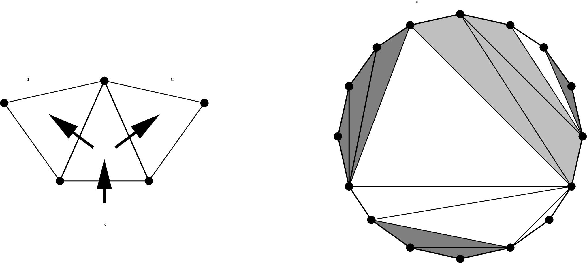
(vi) Polygon gluings.

Let $\Pi=\Pi_{2mn}$ be a regular polygon with $2mn$ sides with a distinguished vertex. An oriented gluing of $\Pi$ is a partition of its sides into $n$ blocks of size $2m$ , with the sides oriented such that as one moves clockwise around $\Pi$ , the orientations in a given block alternate (cf. the right column of Figure 7). We also assume that the first edge in any of these blocks is oriented such that clockwise is positive. The labeling of the edges induces an equivalence relation on the vertices of $\Pi$ , after one performs the identifications. Then $\mathscr{X}_{nm}$ is the set of such gluings with the number of equivalence classes of vertices maximal. A vertex $b$ is a child of $a$ if the edge joining them is positive from $a$ to $b$ . The distinguished vertex is at level $0$ , and the levels of the others are determined by requiring that passing from parent to child increases the level.

4.8.

Figures 6–7 illustrate the combinatorial interpretations used in the computation of $C^{(2)}_{2}=6$ . For this number each object that affords an admissible $2$ -labeling has at most two levels; we show the first level using light grey and the second level using white. Labelings are indicated by the letters $a,b$ . Note that only one object has more than one $2$ -labeling, namely the one appearing in the first three lines of each figure.

4.9 Theorem.

The interpretations (i)–(vi) given in §4.7 count the numbers $C^{(m)}_{n}$ , i.e. (8) holds.

Proof.

First we claim that all the interpretations (i)–(vi) give the same counts. To see this, note that if $\mathscr{X}_{nm}$ is any of the above sets (with no labelings), then $|\mathscr{X}_{nm}|=C_{nm}$ , and there are known bijections between the different objects (cf. [17, Theorem 1.5.1]). For the convenience of the reader, we recall these bijections. To simplify notation we set $m=1$ .

Plane trees and Dyck paths. Let $T$ be a plane tree with $n+1$ vertices with root vertex $v$ . Then $T$ has $n$ edges, and one can build a length $2n$ Dyck path $\pi(T)$ as follows. Recall that a plane tree either consists of the single vertex $v$ , or else $v$ has a sequence of subtrees $T_{1},\dotsc,T_{k}$ , each of which is a plane tree. To construct the Dyck path attached to $T$ , one performs the preorder tree traversal: this is the traversal that begins by visiting the root vertex, then recursively visits the subtrees of the root $T_{1},\dotsc,T_{k}$ , in order. The traversal returns to the root along the root-incident edge every time it is done traversing a subtree.

During the traversal one crosses each edge of $T$ exactly twice, once going down, and once going up. For every move down one appends the step $(1,1)$ to $\pi(T)$ , and for every move up one appends $(1,-1)$ . It is clear that the result is a Dyck path; it has $2n$ steps, never goes below the $x$ -axis, and ends at $(2n,0)$ . One can also easily reverse this process: given a Dyck path $\pi$ , one builds a plane tree $T(\pi)$ whose preorder traversal is encoded by $\pi$ .

Dyck paths and ballot sequences. Let $\pi$ be a Dyck path of length $2n$ . We create a sequence $b(\pi)=(a_{1},\dotsc,a_{2n})$ with $a_{i}\in\{\pm 1\}$ by projecting onto the second coordinate: $(1,1)\mapsto 1$ and $(1,-1)\mapsto-1$ . Thus $b(\pi)$ records the change in height above the $x$ -axis as one moves along $\pi$ . Then $b(\pi)$ is clearly a ballot sequence: the condition that $\pi$ never goes below the $x$ -axis ensures that the partial sums are nonnegative. It is also clear that this process can be reversed to give a map from ballot sequences to Dyck paths.

Plane trees and polygon gluings. Let $T$ be a plane tree. We can regard $T$ as embedded in the sphere $S^{2}$ , for example by applying stereographic projection to the plane. If one cuts the sphere open along the edges of $T$ , one obtains a polygon $\Pi_{2n}$ with $2n$ sides together with data of an oriented gluing: the edges come naturally in pairs, and the root becomes the distinguished vertex of $\Pi_{2n}$ . To go backwards, if one starts with a polygon $\Pi_{2n}$ and identifies the edges in pairs, one obtains a topological surface $S$ together with an embedded connected graph $G$ ( $G$ may have loops or multiple edges). The surface $S$ is orientable if and only if the gluing data is oriented (as one goes around the boundary of the polygon, every pair of edges to be glued must appear with opposite orientations). If $S$ is orientable, then the graph $G$ is a tree if and only if $S$ is a sphere; this happens if and only if the number of vertices of $G$ is maximal after gluing; this follows from considering the Euler characteristic of $S$ , computed as $1-|\text{edges}|+|\text{vertices}|$ .²² 2 As mentioned before (§1.1), there is a connection between polygon gluings and interpretation (59) in [17, Chapter 2]. This interpretation is that $C_{n}$ is the number of ways to draw $n$ nonintersecting chords joining $2n$ points on the circumference of a circle. If one starts with a connected oriented polygon gluing, and draws chords between the centers of the edge pairs, one obtains $n$ chords as in (59). The condition that these chords do not intersect is exactly equivalent to the resulting surface being a sphere.

Triangulations and binary plane trees. Let $\Delta$ be a triangulation of the polygon $\Pi_{n+2}$ with a distinguished edge $e$ . One can make a binary plane tree $B(\Delta)$ by taking the dual of $\Delta$ as follows (cf. Figure 8). The vertices of $B(\Delta)$ are the triangles of $\Delta$ . Two vertices are joined by an edge if and only if they correspond to adjacent triangles in $\Delta$ . The distinguished edge $e$ sits in the boundary of one triangle, which determines the root of $B(\Delta)$ (in Figure 8 the root is indicated by a doubled circle). The resulting tree is embedded in the plane and is a binary tree exactly because each triangle has three sides. It is also easy to see that this construction is reversible.

Plane trees and binary plane trees. Finally we come to this bijection, due to de Bruijn–Morselt [4], which is the most interesting of all. We follow the presentation in the proof of [17, Theorem 1.5.1] closely.³³ 3 In particular we follow the paragraph labeled (iii) $\rightarrow$ (ii) at the bottom of p. 8.

Let $T$ be a plane tree on $n+1$ vertices. We will construct a binary tree $B(T)$ on $n$ vertices; in fact the vertices of $B(T)$ are the non-root vertices of $T$ . First we delete the root from $T$ and all edges incident to it. Then we remove all edges that are not the leftmost edge from any vertex. In other words, if the children of $v$ in $T$ are $v_{1},\dotsc,v_{k}$ , then we remove the edges $\{v,v_{2}\})$ , …, $\{v,v_{k}\}$ and leave the edge $\{v,v_{1}\}$ untouched. After this the remaining edges become the left edges in the binary tree $B(T)$ .

To construct the right edges in $B(T)$ , we create edges horizontally across the vertices of $T$ . In particular, given a vertex $v$ in $T$ , we draw edges from each child $w$ of $v$ to the child of $v$ immediately to the right of $w$ , if this child exists. Finally the root of $B(T)$ is the leftmost child of the root of $T$ . (See Figure 9 for an example.) This process is easily seen to be reversible.

We now return to the original discussion. We claim that for $m>1$ , the same bijections prove that all interpretations give the same counts. One needs only to check that the definitions of admissible labelings are compatible. For instance, to pass from a plane tree $T$ to a Dyck path $\pi$ , one starts at the root of the $T$ and traverses it in preorder (process the node, traverse the left subtree, then traverse the right subtree). As one descends $T$ along an edge, one steps up in $\pi$ by $(1,1)$ , and as one ascends along an edge, one steps down by $(1,-1)$ . With this correspondence, it is evident that the non-root vertices of $T$ coincide with the slabs of $\pi$ . Indeed, the slabs of $\pi$ are constructed so that the corresponding vertices of $T$ are at the same distance from the root, and the poset structure in the slabs mirrors that of the vertices of $T$ . It is also easy to see that the different notions of admissible labelings agree. The verifications for the other interpretations are similar.

To complete the proof, we must check that any one of them actually computes $C_{n}^{(m)}$ . We will use admissibly labeled plane trees (i).

Let $\mathscr{C}=\mathscr{C}_{n+1}$ be the set of pairs

\Bigl\{(T,w)\Bigm|\text{$T\in\mathscr{T}_{n+1}$, $w$ an $a_{T}^{(m)}$-tour}\Bigr\}

modulo the equivalence relation $(T,w)\sim(T^{\prime},w^{\prime})$ if $T=T^{\prime}$ and there is an automorphism of $T$ taking $w$ to $w^{\prime}$ . Then $|\mathscr{C}|=C^{(m)}_{n}$ . Let $\mathscr{P}=\mathscr{P}_{n}$ be the set of plane trees on $n$ vertices, and let $\mathscr{A}=\mathscr{A}_{nm+1}$ be the set of pairs

(9)

\Bigl\{(T,l)\Bigm|\text{ $T\in\mathscr{P}_{nm+1}$ and $l$ is an admissible $m$-labeling of $T$}\Bigr\}.

Then $|\mathscr{A}|$ is the right hand side of (8). We will prove that (8) holds by constructing a bijection between $\mathscr{C}$ and $\mathscr{A}$ .

We begin by defining two maps

\alpha\colon\mathscr{C}\longrightarrow\mathscr{A},\quad\beta\colon\mathscr{A}\longrightarrow\mathscr{C}.

First we define $\alpha$ . Given $(T,w)\in\mathscr{C}$ , let $v$ be the vertex where $w$ begins and ends. Then $\alpha(T,w)$ is the plane tree $\tilde{T}$ whose Dyck word $\pi(\tilde{T})$ is determined by the following rule: the $i$ th step of $\pi(\tilde{T})$ is an up-step if the $i$ th step of $w$ moves towards $v$ , and is a down-step otherwise. We equip $\tilde{T}$ with a labeling $l$ as follows: the $i$ th vertex in preorder traversal of $\tilde{T}$ is given the label of the starting point of the $i$ th edge of $w$ . This labeling $l$ is an admissible $m$ -labeling: if $x_{1},x_{2}$ are two vertices of $\tilde{T}$ with the same labels, then the parents $y_{1},y_{2}$ of $x_{1},x_{2}$ receive the label of the unique vertex $y\in T$ that is one step closer to $v$ . Thus $\alpha(T,w)\in\mathscr{A}$ . We also claim $\alpha$ is well-defined. Suppose $\alpha(T,w)=(\tilde{T},l)$ and $(T,w)\sim(T^{\prime},w^{\prime})$ . Then $\alpha(T^{\prime},w^{\prime})$ is the pair $(\tilde{T},l^{\prime})$ , where the labels of $l^{\prime}$ are a permutation of those of $l$ . Figure 10 shows an example of the computation of $\alpha$ for $m=2$ .

Now we define $\beta$ . Let $(S,l)\in\mathscr{A}$ . Let $\bar{S}$ be the graph obtained from $S$ by first identifying any two vertices of $S$ that share the same label, and then by replacing parallel edges in the resulting multigraph by single edges. We note that $\bar{S}$ is actually a tree. Indeed, the admissibility of the labeling implies that the map $E(S)\rightarrow E(\bar{S})$ on edges is $m:1$ , and the map on vertices is $m:1$ away from the root and $1:1$ on the root. Thus $\bar{S}$ has $n+1$ vertices and $n$ edges, and since it is clearly connected $\bar{S}$ is a tree. Finally, we define a walk $w=w(\bar{S})$ on $\bar{S}$ by writing the sequence of labels encountered during the preorder traversal of $S$ . The $m$ -admissibility of the labeling implies that $w$ is an $a^{(m)}_{S}$ -tour, and thus we have defined an element $\beta(S,l)=(\bar{S},w)$ . Figure 11 shows an example of this construction.

To complete the proof, we must show that $\alpha$ , $\beta$ are bijections. First we show $\beta\circ\alpha=1_{\mathscr{C}}$ . We claim that if $(\bar{S},w(\bar{S}))=(\beta\circ\alpha)(T,w)$ , then $\bar{S}=T$ and $w(\bar{S})=w$ (in other words, the representative of an equivalence class in $\mathscr{C}$ is taken to itself). This is clearly true if $T$ has one vertex. Suppose the claim is true for all pairs $(T,w)$ with $\leq n$ vertices. Let $T$ be a tree with $n+1$ vertices, let $w$ be an $a_{T}^{(m)}$ -tour of $T$ beginning at $v$ , let $x$ be a leaf of $T$ , and let $y$ be the neighbor of $x$ in $T$ . Deleting $x$ and modifying $w$ appropriately we obtain a pair $(T^{\prime},w^{\prime})$ . In $(S^{\prime},l^{\prime})=\alpha(T^{\prime},w^{\prime})$ we have $m$ vertices $y_{1},\dotsc,y_{m}$ corresponding to $y$ . Then $(S,l)=\alpha(T,w)$ is obtained from $(S^{\prime},l^{\prime})$ by placing $m$ new vertices $x_{1},\dotsc,x_{m}$ under the $y_{i}$ according to where they appear in the walk $w$ . By induction $\beta(S^{\prime},l^{\prime})=(T^{\prime},w^{\prime})$ . When we construct $\beta(S,l)$ the only differences are that now we collapse the $m$ edges of the form $(x_{i},y_{j})$ to a single edge in $\bar{S}$ joining $x$ to $y$ , and that we build $w(\bar{S})$ from $w(\bar{S}^{\prime})$ by incorporating the vertex $x$ . Clearly $\bar{S}=T$ . Moreover $w(\bar{S})=w$ , since the edges in $S$ were built to make preorder traversal in $S$ match the original walk $w$ . This shows $\beta\circ\alpha=1_{\mathscr{C}}$ .

Now we show $\alpha\circ\beta=1_{\mathscr{A}}$ . The proof is similar. Clearly this is true for all $(S,l)\in\mathscr{A}$ with one vertex. Suppose that for all $(S,l)$ with $<nm+1$ vertices we have $(\alpha\circ\beta)(S,l)=(S,l)$ . Let $(S,l)$ have $nm+1$ vertices and choose a leaf $x_{1}$ of $S$ of highest level. The admissibility of the labeling $l$ implies that there are $m-1$ additional vertices $x_{2},\dotsc,x_{m}$ with the same label as $x_{1}$ , and since $x_{1}$ lies in the highest level, the vertices $x_{2},\dotsc,x_{m}$ must also be leaves of $S$ . Let $y_{1},\dotsc,y_{m}$ be the vertices of $S$ with label equal to any parent of $x_{i}$ . In particular, the parents of the $x_{i}$ are a subset of the $y_{j}$ , but not every $y_{j}$ is necessarily a parent of an $x_{i}$ . Deleting the $x_{i}$ we obtain a labeled plane tree $(S^{\prime},l^{\prime})$ . If $(\bar{S}^{\prime},w(\bar{S}^{\prime}))=\alpha(S^{\prime},l^{\prime})$ , then by induction we have $\beta(\bar{S}^{\prime},w(\bar{S}^{\prime}))=(S^{\prime},l^{\prime})$ , and moreover the tree $\bar{S}^{\prime}$ is obtained from $\bar{S}$ by deleting $x$ (the image of the $x_{i}$ ). The walk $w(\bar{S})$ is obtained from $w(\bar{S}^{\prime})$ by inserting steps along the edge $(x,y)$ exactly according to the up- and down-steps in $S$ along the edges of the form $(x_{i},y_{j})$ , where $y$ is the image of the $y_{j}$ . After applying $\alpha$ we exactly recover the edges $(x_{i},y_{j})$ in $S$ . This shows $\alpha\circ\beta=1_{\mathscr{A}}$ , and completes the proof of the theorem. ∎

4.10 Remark.

The interpretations in Theorem 4.9 make it possible to define various higher analogues of other standard numbers, such as Narayana numbers, and higher $q$ -analogues. We have not pursued these definitions.

5. Generating functions and asymptotics

5.1.

Let

(10)

F_{m}(x)=\sum_{n\geq 0}C^{(m)}_{n}x^{n}

be the ordinary generating function of the $C^{(m)}_{n}$ . In this section we explain how to use the combinatorial interpretations in §4 to compute (10) to arbitrary precision as a power series in $x$ . Then we will give a conjecture of the asymptotic behavior of $C^{(m)}_{n}$ that generalizes the famous formula

C_{n}\sim\frac{4^{n}}{n^{3/2}\sqrt{\pi}},\quad(n\rightarrow\infty).

5.2.

We will compute $F_{m}(x)$ by showing that counting admissibly labeled plane trees on $nm+1$ vertices is equivalent to counting colored plane trees on $n+1$ vertices. To count the latter, we use standard generating function techniques as described in Flajolet–Sedgewick [8]. For the benefit of the reader and to keep our presentation as self-contained as possible, we recall the results we need here.

5.3 Proposition.

(i)

Let $A(x)=\sum_{k\geq 0}a_{k}x^{k}\in\mathbb{Z}[\![x]\!]$ be an integral formal power series with $a_{k}\geq 0$ . Let $\mathscr{P}_{A}$ be the set of all colored plane trees such that any vertex with $k$ children can be painted one of $a_{k}$ colors. Let $P_{A}\in\mathbb{Z}[\![x]\!]$ be the ordinary generating function of $\mathscr{P}_{A}$ , so that the coefficient $[x^{n}]P_{A}(x)$ of $x^{n}$ counts the trees in $\mathscr{P}_{A}$ with $n$ vertices. Then $P_{A}$ satisfies the functional relation

(11) $P_{A}=xA(P_{A}).$
(ii)

Let $B(x)=\sum_{k\geq 0}b_{k}x^{k}\in\mathbb{Z}[\![x]\!]$ be another integral formal power series with $b_{k}\geq 0$ . Let $\mathscr{P}_{A,B}$ be the set of all colored plane trees such that (a) any non-root vertex with $k$ children can be painted one of $a_{k}$ colors, and (b) if the root vertex has degree $k$ then it can be painted any one of $b_{k}$ colors. Let $P_{A,B}\in\mathbb{Z}[\![x]\!]$ be the ordinary generating function of $\mathscr{P}_{A,B}$ . Then $P_{A,B}$ satisfies the functional relation

(12) $P_{A,B}=xB(P_{A}),$

where $P_{A}$ satisfies (11).

Proof.

These results are proved in [8]. Specifically (i) is [8, Proposition I.5] and (ii) follows from [8, Example III.8]. We sketch the proof here.

For (11), recall that a plane tree is a rooted tree with an ordering specified for the children of each vertex. This is equivalent to the recursive specification that a plane tree is a root vertex $v$ with a (possibly empty) sequence of plane trees $T_{1},\dotsc,T_{k}$ attached in order to $v$ , with the root of $T_{i}$ becoming the $i$ th child of $v$ . If $P$ is the ordinary generating function of plane trees, this description leads to the well-known functional relation

P=x(1+P+P^{2}+P^{3}+\dotsb),

where the right hand side encodes the process of attaching an arbitrary sequence of plane trees to an initial root vertex.

Now consider the collection $\mathscr{P}_{A}$ of plane trees colored according to $A$ . In terms of the recursive specification above, one can think of building a tree in $\mathscr{P}_{A}$ by (i) picking a root vertex $v$ and deciding on the number $k$ of its children, (ii) coloring $v$ one of $a_{k}$ different colors, and (iii) continuing the process recursively to each of the $k$ children of $v$ . This leads to the functional relation

P_{A}=x(a_{0}+a_{1}P_{A}+a_{2}P_{A}^{2}+a_{3}P_{A}^{3}+\dotsb),

which proves (11).

To see (12), we note that a tree in $\mathscr{P}_{A,B}$ is built similarly. We (i) choose a root vertex $v$ and decide on the number $k$ of its children, (ii) color $v$ one of $b_{k}$ different colors, and (iii) place trees from $\mathscr{P}_{A}$ under $v$ with their roots as $v$ ’s children. This leads to

P_{A,B}=x(b_{0}+b_{1}P_{A}+b_{2}P_{A}^{2}+b_{3}P_{A}^{3}+\dotsb),

which proves (12). ∎

5.4 Definition.

If $S$ is a plane tree appearing in $\mathscr{P}_{A,B}$ , then we say $S$ has been equipped with an $(A,B)$ -coloring.

5.5.

Now we define the generating functions for the colorings we will need. For any pair $g\geq 0,r\geq 1$ , let $\lambda(r,g)$ be the dimension of the space of degree $g$ homogeneous polynomials in $r$ variables. We have

\lambda(r,g)=\binom{r-1+g}{r-1}.

For any $k\geq 0$ , let $W_{m}(k)$ be the number of partitions of a set of size $k$ into blocks of size $m$ . Then $W_{m}(k)=0$ unless $m$ divides $k$ , and in this case we have

W_{m}(k)=\frac{k!}{(m!)^{k/m}(k/m)!}.

5.6 Theorem.

Put

\ell_{m}(x)=\sum_{d\geq 0}W_{m}(dm)\lambda(m,dm)x^{d}

and

h_{m}(x)=\sum_{d\geq 0}W_{m}(dm)x^{d}.

Let $f_{m}(x)\in\mathbb{Z}[\![x]\!]$ satisfy the functional equation

(13)

f_{m}(x)=x\ell_{m}(f_{m}(x)).

Then the generating function $F_{m}(x)=\sum_{n\geq 0}C^{(m)}_{n}x^{n+1}$ satisfies

(14)

F_{m}(x)=xh_{m}(f_{m}(x)).

Proof.

Let us fix $m\geq 1$ and simplify notation by writing $F$ , $f$ , $\ell$ , $h$ instead of $F_{m}$ , $f_{m}$ , $\ell_{m}$ , $h_{m}$ . Then by Proposition 5.3 $F$ is the ordinary generating function of the $(\ell,h)$ -colored plane trees $\mathscr{P}_{\ell,h}$ . Recall (9) that $\mathscr{A}$ is the set of pairs $(T,l)$ where $T\in\mathscr{P}_{nm+1}$ and $l$ is an admissible $m$ -labeling of $T$ . We will construct a surjective map

(15)

\rho\colon\mathscr{A}\longrightarrow\mathscr{P}

show that it induces a bijection between trees $(\ell,h)$ -colored plane trees with $n+1$ vertices and admissibly $m$ -labeled plane trees $\mathscr{A}_{nm+1}$ on $nm+1$ vertices. First we assume that the labeling set $L$ is the positive integers $\mathbb{Z}_{\geq 0}$ , with its standard total order. Then we assume that $(S,l)\in\mathscr{A}$ is labeled so that the following properties hold:

(i)

If $S$ has $nm+1$ vertices, then $l$ is surjective onto $[\![n]\!]\subset L$ .
(ii)

If $x,y\in S$ are two vertices and $y$ is in a higher level than $x$ (i.e. $y$ is further from the root than $x$ ), then $l(x)<l(y)$ .
(iii)

If $x,x^{\prime}\in S$ are on the same level with $l(x)<l(x^{\prime})$ , and $y$ (respectively, $y^{\prime}$ ) is a child of $x$ (resp., $x^{\prime}$ ), then $l(y)<l(y^{\prime})$ .
(iv)

If $L^{\prime}\subset L$ is the subset of labels appearing in a fixed level of $S$ , then the elements of $L^{\prime}$ are ordered compatibly with when they first appear when read from left to right: the leftmost vertex receives the smallest label from $L^{\prime}$ , the first new label seen when reading to the right is next largest available label from $L^{\prime}$ , and so on until the final label in $L^{\prime}$ is seen.

It is clear that, given any admissibly $m$ -labeled tree, one can permute the labels to satisfy these properties, and that the resulting labeling is unique.

Recall that in the proof of Theorem 4.9, we built a topological tree $\bar{S}$ on $n+1$ vertices from $S$ by identifying vertices with the same labels and replacing parallel edges with single edges. After fixing a total order on $L$ and requiring that the labels of $S$ satisfy the above, we obtain a canonical plane tree structure on $\bar{S}$ . The root of $\bar{S}$ is the image of the root of $S$ , and each non root vertex of $\bar{S}$ receives a unique label from $1$ to $n$ . The children of any vertex are ordered using the order in $[\![n]\!]\subset\mathbb{Z}_{>0}$ . In the resulting plane tree, which we also denote by $\bar{S}$ , the labels in a given level increase when read from left to right, and labels in higher levels are larger than those in lower levels. In particular, the labeling of $\bar{S}$ is uniquely determined; for this discussion, we will say that the plane tree $\bar{S}$ has been canonically labeled. Figure 12 shows an example of an admissibly $2$ -labeled plane tree $S$ satisfying the conditions (i)–(iv), and the resulting canonically labeled plane tree $\bar{S}$ .

We have thus constructed the map $\rho$ in (15). We claim $\rho$ is surjective. We let $\bar{S}$ be a canonically labeled plane tree, and we build an admissibly $m$ -labeled tree $(S,l)\in\rho^{-1}(\bar{S})$ as follows. Suppose $\bar{v}\in\bar{S}$ is the root with children $x_{1},\dotsc,x_{d}$ , read from left to right. Under the root $v\in S$ we place $dm$ vertices

(16)

x_{1}^{(1)},\dotsc,x_{1}^{(m)},\dotsc,x_{d}^{(1)},\dotsc,x_{d}^{(m)},

from left to right with $l(x_{i}^{(j)})=l(x_{i})$ , and put $\rho(x_{i}^{(j)})=\rho(x_{i})$ . Now suppose $\bar{v}\in\bar{S}$ is a non root vertex with $d$ children. By induction on distance to the root, we may assume that $\bar{v}$ has already been lifted to $m$ vertices $v^{(1)},\dotsc,v^{(m)}$ with $l(v^{(i)})=l(\bar{v})$ , and these vertices have been placed in their level in $S$ in some order. We lift the children $x_{1},\dotsc,x_{d}$ of $\bar{v}$ to $dm$ vertices as before, again with $l(x_{i}^{(j)})=l(x_{i})$ and $\rho(x_{i}^{(j)})=\rho(x_{i})$ , and we make them all children of $v_{1}^{(1)}$ in the order (16). Continuing in this way we obtain an admissibly $m$ -labeled $(S,l)\in\rho^{-1}(\bar{S})$ with $l$ satisfying (i)–(iv), which shows $\rho$ is surjective.

To complete the proof, we claim that the inverse image $\rho^{-1}(\bar{S})$ is in bijection with the $(\ell,h)$ -colorings of $\bar{S}$ . To see this we revisit the proof of surjectivity and see what additional choices one could make along the way to build $(S,l)$ . First consider the root vertex $\bar{v}\in\bar{S}$ and suppose it has $d$ children $x_{1},\dotsc,x_{d}$ . As before we lift these children to $dm$ vertices $x^{(1)}_{1},\dotsc,x_{d}^{(m)}$ under the root $v\in S$ , but we are not obligated to order them as in (16). We can use any order compatible with the induced ordering of the labels of the $x_{1},\dotsc,x_{d}$ and with the requirements (i)–(iv). In particular this implies that these orders are in bijection with set partitions of $[\![dm]\!]$ into $d$ blocks $B_{1},\dotsc,B_{d}$ of size $m$ : if the vertices $x_{i}^{(j)}$ are ordered under $v$ as $y_{1},\dotsc,y_{dm}$ , then

l(y_{i})=k\quad\text{if and only if}\quad i\in B_{k}.

Since there are $W_{m}(dm)$ such set partitions, we see that the root must be colored according to $h$ .

Now consider a non root vertex $\bar{v}$ with $d$ children $x_{1},\dotsc,x_{d}$ . Again by induction we know that the vertices $v^{(1)},\dotsc,v^{(m)}$ mapping to $\bar{v}$ have been placed in order in their level in $S$ . To place the $dm$ vertices $x_{1}^{(1)},\dotsc,x_{d}^{(m)}$ in their level we must do two things:

(A)

We must choose an order of the $x_{i}^{(j)}$ in their level, and this order must be compatible with $l(x_{i}^{(j)})=l(x_{i})$ and the requirements (i)–(iv).
(B)

After fixing the order of the $x_{i}^{(j)}$ , we must decide how to place them under their (potential) parents $v^{(1)},\dotsc,v^{(m)}$ .

As before (A) corresponds to a set partition of $[\![dm]\!]$ into $d$ blocks of size $m$ . The data in (B) corresponds to an order preserving map from $[\![dm]\!]$ to $[\![m]\!]$ : if $x\in\{x_{i}^{(j)}\}$ is a child of $v\in\{v^{(j)}\}$ , then any $x^{\prime}>x$ (according to the order chosen in (A)) cannot be a child of any $v^{\prime}<v$ . Such maps are counted by $\lambda(m,dm)$ . Indeed, a degree $dm$ monomial $z_{1}^{e_{1}}\dotsb z_{m}^{e_{m}}$ encodes that the first $e_{1}$ in $[\![dm]\!]$ map to $1\in[\![m]\!]$ , the next $e_{2}$ map to $2$ , and so on. This means the total number of choices is $W_{m}(dm)\cdot\lambda(m,dm)$ , which implies that any non root vertex with $d$ children must be colored according to $\ell$ .

We have thus shown that any $(S,l)$ in the inverse image $\rho^{-1}(\bar{S})$ corresponds uniquely to an $(\ell,h)$ -coloring of $\bar{S}$ . By Proposition 5.3, this completes the proof. ∎

5.7 Remark.

At this point the reader may be nostalgic for the recurrence relation satisfied by the classical Catalan numbers, which corresponds to the equation

(17)

xF_{1}^{2}-F_{1}+1=0.

For $m>1$ , the power series $F_{m}(x)$ does not appear to be algebraic, so unfortunately one does not have such a simple recurrence relation on its coefficients. However, experimentally one finds that there is an algebraic relation satisfied by $f_{m}$ and $F_{m}$ :

(18)

f_{m}^{2}-xF_{m}+x=0.

Relation (18) is easily checked when $m=1$ . We have $f_{1}=xF_{1}$ , so (18) is really the same as (17). For $m>1$ a proof of (18) was given by Mark Wilson [19]. One observes that $\ell_{m}$ and $h_{m}$ are related by

x\ell_{m}(x)=h_{m}(x)-1,

from which (18) easily follows.

The relation (18) gives a connection between pairs of objects computing hypergraph Catalan numbers in the spirit of that encoded by (17). Consider $m=2$ . We have

f_{2}(x)=x+3x^{2}+24x^{3}+267x^{4}+\dotsb,

and

f_{2}(x)^{2}=x^{2}+6x^{3}+57x^{4}+678x^{5}+\dotsb=x(F_{2}(x)-1).

We see $C_{3}^{(2)}=57$ as the coefficient of $x^{4}$ in $f_{2}(x)^{2}$ , which comes from the coefficients of $x,x^{2},x^{3}$ in $f_{2}(x)$ via

(19)

57=24\cdot 1+3\cdot 3+1\cdot 24.

This is certainly reminiscent of the classical Catalan relation, although there is an important difference. The numbers involved on the right of (19) are connected with $C^{(2)}_{2},C^{(2)}_{3},C^{(4)}_{2}$ , but they enumerate proper subsets of the associated objects, not the full sets. Indeed, this is obviously true, since both sides of (19) involve the same number $C^{(2)}_{3}$ ! We have not attempted to explore this connection further.

5.8.

We conclude this section by discussing asymptotics for the $C^{(m)}_{n}$ . The results here are purely experimental; none have been proved, although based on our numerical experiments we are confident in them. We learned this technique from Don Zagier, who calls it multiplying by $n^{8}$ ; an excellent lecture by him at ICTP demonstrating the method can be found online [20].

Suppose one has a sequence $a=\{a_{n}\}_{n\geq 0}$ that one believes satisfies an asymptotic of the form

(20)

a_{n}\sim C_{0}+C_{1}/n+C_{2}/n^{2}+\dotsb\quad(n\rightarrow\infty).

It may be difficult to extract $C_{0}$ to high precision even when $n$ is large, since $C_{1}/n$ might still be non-negligible. However it is possible to wash away the contributions of the nonconstant terms $C_{k}/n^{k}$ , $k\geq 1$ . One multiplies both sides of (20) by $n^{8}$ (or any other reasonable even power of $n$ ), and then applies the difference operator $(8!)^{-1}\Delta^{8}$ to both sides, where $\Delta a$ is the sequence $(\Delta{a})_{n}:=a_{n+1}-a_{n}$ . The operator $\Delta^{k}$ annihilates any polynomial $p(n)$ of degree $<k$ , takes $n^{k}$ to $k!$ , and takes $n^{-l}$ to a rational function in $n$ of degree $-l-k$ .⁴⁴ 4 Here the degree of a rational function $P/Q$ in one variable means $\deg P-\deg Q$ . Let $b=\{b_{n}\}$ be the sequence resulting from multiplying $a_{n}$ by $n^{8}/8!$ and applying the difference operator $\Delta$ eight times. Then we have

(21)

b_{n}\sim C_{0}+C_{9}p_{-9}(n)+C_{10}p_{-10}(n)+\dotsb,

where $p_{-k}(n)$ denotes a rational function in $n$ of degree $-k$ . If one then evaluates the left of (21) at a large value of $n$ , the effects of $C_{k}$ , $k\geq 9$ are negligible on the right and one clearly sees $C_{0}$ . One can then repeat the process with the sequence $n(a_{n}-C_{0})$ to find $C_{1}$ , and so on.

5.9.

We illustrate with the series $F_{2}(x)=1+x+6x^{2}+57x^{3}+678x^{4}+\dotsb$ . Playing with the data one makes the ansatz

(22)

C^{(2)}_{n}\sim KA^{n}\,n!\,n^{\rho}

for some constants $K,A,\rho$ . Indeed, apart from the $n!$ , the right of (22) is typical for these kinds of problems, and was our initial guess; it quickly became evident that $n!$ needed to be included. The series

a_{n}:=C^{(2)}_{n}/n!

should then appear to grow exponentially, and the sequence of ratios $\{a_{n}/a_{n-1}\}$ should satisfy (20) with $C_{0}=A$ . Indeed, using 100 terms of $F_{2}$ and $\Delta^{16}$ we get

A\approx 2.0000000000068961809\dotsb.

Next we consider the sequence

a_{n}:=C^{(2)}_{n}/(2^{n}\,n!),

which we expect to be asymptotic to $Kn^{\rho}$ . We can detect $\rho$ using the sequence $b_{n}=(\Delta\log a)_{n}/(\log(n+1)-\log n)$ , which satisfies (20) with $C_{0}=-\rho$ . Again with 100 terms and $\Delta^{16}$ we get

-\rho\approx 0.499999997726715\dotsb.

Hence we have

C_{n}^{(2)}\sim K\cdot\frac{2^{n}\,n!}{\sqrt{n}}

and we must find the constant $K$ . We consider $b_{n}=C^{(2)}_{n}\sqrt{n}/2^{n}n!$ and look for $C_{0}$ . This time finding $K$ is more difficult. Taking 200 terms and applying $\Delta^{16}$ , this number appears to be $5.05704458036912766\dotsb$ . We use the Inverse Symbol Calculator [2], which attempts to symbolically reconstruct a given real number using various techniques, and find

K\approx 2e^{3/2}/\sqrt{\pi}.

(The $e^{3/2}$ is surprising, but is apparently correct. Using 600 terms of the sequence, we find that $K\sqrt{\pi}/2$ agrees with $e^{3/2}$ with relative error $<10^{-76}$ .) The conclusion is

C_{n}^{(2)}\mathbin{{\mathop{\sim}\limits}}e^{3/2}\cdot\frac{2^{n+1}\,n!}{\sqrt{\pi n}},\quad(n\rightarrow\infty).

We present asymptotics for the $C^{(m)}_{n}$ as a conjecture:

5.10 Conjecture.

Let $m>1$ . Then as $n\rightarrow\infty$ , we have

C_{n}^{(m)}\sim K_{m}\cdot\frac{\bigl(\frac{m^{m-1}}{(m-1)!}\bigr)^{n+1}\,(n!)^{m-1}}{(\pi n)^{(m-1)/2}},

where the constant $K_{m}$ is defined by

K_{m}=\begin{cases}e^{3/2}&\text{if $m=2$,}\\ 2\binom{2}{2}\binom{4}{2}\dotsb\binom{m-1}{2}/m^{(2m-3)/2}&\text{if $m\geq 3$ and is odd, and}\\ \sqrt{2}\binom{3}{2}\binom{5}{2}\dotsb\binom{m-1}{2}/m^{(2m-3)/2}&\text{if $m\geq 4$ and is even.}\end{cases}

5.11 Remark.

We have tested Conjecture 5.10 numerically using 100 terms of $F_{m}(x)$ for all $m\leq 30$ . We have not systematically tried to find higher terms in the asymptotic expansion of $C_{n}^{(m)}$ , as in (20).

6. Connection with matrix models

6.1.

We finish by explaining how the numbers $C_{n}^{(m)}$ are related to hypergraphs and matrix models [5]. We first explain the connection between graphs, matrix models, and the usual Catalan numbers. For more information, we refer to Harer–Zagier [9], Etingof [6, §4], Lando–Zvonkin [10], and Eynard [7].

6.2.

Let $d\mu_{2}(x)$ be the measure on polynomial functions on $\mathbb{R}$ with moments

\left\langle x^{r}\right\rangle_{2}:=\int_{\mathbb{R}}x^{r}d\mu_{2}(x)=W_{2}(r),

where $W_{2}(r)$ is the number of pairings on a set of size $r$ . It is well-known that $d\mu_{2}(x)$ is essentially the Gaussian measure, up to normalization: we have

\left\langle x^{r}\right\rangle_{2}=(2\pi)^{-1/2}\int_{\mathbb{R}}x^{r}e^{-x^{2}/2}\,dx,

where $dx$ is the usual Lebesgue measure on $\mathbb{R}$ .

Let $g_{1},g_{2},\dotsc$ be a family of indeterminates, and let $S(x)$ be the formal power series $\sum_{r\geq 1}g_{r}x^{r}/r!$ . We can compute the expectation $\left\langle\exp(S(tx))\right\rangle_{2}$ as a formal power series in $t$ with coefficients in the polynomial ring $\mathbb{Q}[g_{1},g_{2},\dotsc]$ . We have

(23)

\left\langle\exp S(tx)\right\rangle_{2}=1+A_{2}t^{2}/2+A_{4}t^{4}/8+A_{6}t^{6}/48+\dotsb

where

A_{2}=g_{1}^{2}+g_{2},\quad A_{4}=g_{1}^{4}+6g_{1}^{2}g_{2}+4g_{1}g_{3}+3g_{2}^{2}+g_{4},\\ A_{6}=g_{1}^{6}+15g_{1}^{4}g_{2}+20g_{1}^{3}g_{3}+45g_{1}^{2}g_{2}^{2}+15g_{1}^{2}g_{4}\\ +60g_{1}g_{2}g_{3}+6g_{1}g_{5}+15g_{2}^{3}+15g_{2}g_{4}+10g_{3}^{2}+g_{6}.

The series (23) can be interpreted as a generating function for graphs weighted by the inverse of the orders of their automorphism groups (cf. [6, Theorem 3.3]). Let $\mathbf{n}=(n_{1},n_{2},\dotsc)$ be a vector of nonnegative integers, with $n_{i}$ nonzero only for finitely many $i$ . Let $|\mathbf{n}|=\sum n_{i}$ . We say a graph $\gamma$ has profile $\mathbf{n}$ if it has $n_{i}$ vertices of degree $i$ . Let $G(\mathbf{n})$ be the set of all graphs of profile $\mathbf{n}$ , up to isomorphism (we allow loops and multiple edges). By an automorphism of a graph, we mean a self-map that permutes edges and vertices. In particular, automorphisms include permuting multiedges between two vertices, and flipping loops at a vertex (exchanging the two half-edges emanating from the vertex that form the loop). For any $\gamma\in G(\mathbf{n})$ , let $\Gamma(\gamma)$ be its automorphism group. Then we have

\left\langle\exp S(tx)\right\rangle_{2}=\sum_{\mathbf{n}}t^{|\mathbf{n}|}\sum_{\gamma\in G(\mathbf{n})}\frac{\prod_{i}g_{i}^{n_{i}}}{|\Gamma(\gamma)|}.

For example, consider the term $5g_{3}^{2}/24$ from $A_{6}$ in (23). There are two graphs with this profile, shown in Figure 13. The left has $2\cdot 2\cdot 2$ automorphisms, and the right has $2\cdot 3!$ , which gives $1/8+1/12=5/24$ .

6.3.

Now we want to replace the Gaussian measure, which is connected to counting pairings of a set, with something that is connected to the numbers $W_{2m}(r)$ , which count set partitions of $[\![r]\!]$ with blocks of size $2m$ . Let $d\mu_{2m}(x)$ be the “measure” on polynomial functions on $\mathbb{R}$ that gives the monomial $x^{r}$ the expectation $W_{2m}(r)$ . More precisely, we consider the function taking $x^{r}$ to $W_{2m}(r)$ and extend linearly to polynomials. This is not a measure in the usual sense, although formally we can regard it as such. The “expectation” $\left\langle\exp S(tx)\right\rangle_{2m}$ is then a well-defined power series in $t$ , and has a combinatorial interpretation via hyperbaggraphs.

Recall that a hypergraph on a vertex set $V$ — a notion due to Berge [1] — is a collection of subsets of $V$ , called the hyperedges. The degree of a vertex is the number of hyperedges it belongs to, and a hypergraph is regular if these numbers are the same for all vertices. The order of a hyperedge is its number of vertices. If all hyperedges have the same order, we say that the hypergraph is uniform.

Now suppose we allow $V$ to be a multiset, in other words a set with a multiplicity map $V\rightarrow\mathbb{Z}_{\geq 1}$ . Then these constructions lead to hyperbaggraphs, due to Ouvrard–Le Goff–Marchand-Maillet [13].(⁵⁵ 5 In the CS literature, multisets are sometimes called bags.) We extend the notions of regularity and uniformity above by incorporating the multiplicity in an obvious way (the order of a subset of a multiset is sum of the multiplicities of its elements).

With these definitions, the expectation $\left\langle\exp S(tx)\right\rangle_{2m}$ now enumerates uniform hyperbaggraphs of all profiles weighted by the inverses of their automorphism groups, where each hyperedge has $2m$ elements. For example,

(24)

\left\langle\exp S(tx)\right\rangle_{4}=1+B_{4}t^{4}/24+B_{8}t^{8}/1152+\dotsb

where

B_{4}=g_{1}^{4}+6g_{1}^{2}g_{2}+4g_{1}g_{3}+3g_{2}^{2}+g_{4},\quad B_{8}=g_{1}^{8}+28g_{1}^{6}g_{2}+56g_{1}^{5}g_{3}+\dotsb+35g_{4}^{2}+g_{8}.

The computation of the contribution $35g_{4}^{2}/1152$ from $B_{8}$ in (24) is as follows. There are three hyperbaggraphs of this profile, each with two hyperedges. The underlying set of vertices has $2$ elements $a$ , $b$ , and we represent a hyperedge by a monomial in these variables. The profile $g_{4}^{2}$ means that each vertex has degree $4$ , and since $2m=4$ we must have uniformity $4$ . Thus we want pairs of monomials in $a,b$ of total degree $4$ . This gives

(25)

\{a^{4},b^{4}\},\quad\{a^{3}b,ab^{3}\},\quad\{a^{2}b^{2},a^{2}b^{2}\}.

The orders of the automorphism groups are

(26)

2\cdot(4!)^{2},\quad 2\cdot(3!)^{2},\quad 2\cdot 2\cdot(2!)^{2}(2!)^{2}.

For example, the automorphisms of the last hyperbaggraph come from interchanging the vertices, interchanging the two hyperedges, and the internal flips within the hyperedges; the last type of automorphism cannot occur for graphs. Adding the inverses of these orders, one finds $1/1152+1/72+1/64=35/1152$ , which agrees with $B_{8}$ above.

As a final remark, we note that $A_{4}=B_{4}$ . This is a general phenomenon: one can show that the coefficient of $t^{n}$ in $\left\langle\exp S(tx)\right\rangle_{2m}$ is the complete exponential Bell polynomial $\mathbf{Y}_{n}(g_{1},\dotsc,g_{n})$ , divided by $(2m)!^{d}\,d!$ , where $d=n/2m$ . We refer to [3, p. 134, eqn. 3b] for the definition of these; the coefficients of the $\mathbf{Y}_{n}$ can be found on OEIS as sequence A178867.

6.4.

Now we pass to matrix models. Let $V=V_{N}$ be the real vector space of $N\times N$ complex Hermitian matrices. The space $V$ has real dimension $N^{2}$ . For any polynomial function $f\colon V\rightarrow\mathbb{R}$ , define

(27)

\left\langle f\right\rangle=C^{-1}\int_{V}f(X)\exp(-\Tr X^{2}/2)\,dX,

where $\Tr(X)=\sum_{i}X_{ii}$ is the sum of diagonal entries and the constant $C$ is determined by the normalization $\left\langle 1\right\rangle=1$ . The measure $\exp(-\Tr X^{2}/2)\,dX$ is essentially the product of the Gaussian measures $d\mu_{2}(x)$ from §6.2 taken over the real coordinates of $V$ . The only difference is that for any off-diagonal entry $Z_{ij}=X_{ij}+\sqrt{-1}Y_{ij}$ , we have rescaled the measure so that for even $r$ we have $\left\langle X_{ij}^{r}\right\rangle_{2}=\left\langle Y_{ij}^{r}\right\rangle_{2}=W_{2}(r)/2^{r/2}$ .

Now consider (27) evaluated on the polynomial given by taking the trace of the $r$ th power:

(28)

P(N,r)=\left\langle\Tr X^{r}\right\rangle.

For $r$ odd (28) vanishes for all $N$ . On the other hand, for $r$ even and $N$ fixed, it turns out that $P(N,r)$ is an integer, and as a function of $N$ is a polynomial of degree $r/2+1$ with integral coefficients.

Furthermore, the number $P(N,r)$ has the following remarkable combinatorial interpretation. Let $\Pi_{r}$ be a polygon with $r$ sides. Any pairing $\pi$ of the sides of $\Pi_{r}$ determines a topological surface $\Sigma(\pi)$ endowed with an embedded graph (the images of the edges and vertices of $\Pi_{r}$ ). Let $v(\pi)$ be the number of vertices in this embedded graph. Then we have

(29)

P(N,r)=\sum_{\pi}N^{v(\pi)},

where the sum is taken over all oriented pairings of the edges of $\Pi_{r}$ such that the resulting topological surface $\Sigma_{\pi}$ is orientable. For example, we have

(30)

P(N,0)=N,P(N,2)=N^{2},P(N,4)=2N^{3}+N,\\ P(N,6)=5N^{4}+10N^{2},\quad P(N,8)=14N^{5}+70N^{3}+21N.

The pairings yielding $P(N,4)$ are shown in Figure 14.

6.5.

One can see from (30) that the leading coefficient of $P(N,r)$ is none other than the Catalan number $C_{r/2}$ . This follows easily from the interpretation of the Catalan numbers in terms of polygon gluings ((vi) from §4.7). Indeed, the leading coefficient counts the number of oriented pairings of $\Pi_{r}$ such that the number of vertices $v(\pi)$ in the orientable surface $\Sigma_{r}$ is maximal; this is exactly the interpretation above.

6.6.

Now we modify the matrix model. We replace the Gaussian measure

\exp(-\Tr X^{2}/2)\,dX

by the product of the formal measures $d\mu_{2m}(x)$ taken over the real coordinates; again we rescale on the off-diagonal coordinates so that for $r\equiv 0\bmod 2m$ we have $\left\langle X_{ij}^{r}\right\rangle_{2m}=\left\langle Y_{ij}^{r}\right\rangle_{2m}=W_{2m}(r)/2^{r/(2m)}$ . We write the corresponding formal measure by $d\mu_{2m}(X)$ . Then we obtain a new matrix model where polygons are glued by grouping their edges into subsets of size $2m$ instead of pairs. As above one can see that for $r\equiv 0\bmod 2m$ , the integrals

(31)

\int_{V}\Tr X^{r}\,d\mu_{2m}(X)

are polynomials $P_{2m}(N,r)$ in the dimension $N$ . For example, when $2m=4$ we have

P_{4}(N,4)=N^{2},\quad P_{4}(N,8)=6N^{3}+21N^{2}+8N,\\ P_{4}(N,12)=57N^{4}+715N^{3}+2991N^{2}+2012N.

The hypergraph Catalan numbers $C_{r}^{(m)}$ are the leading coefficients of these polynomials: we have

P_{2m}(N,2mr)=C_{r}^{(m)}N^{r+1}+\dotsb.

A direct computation with the definition (31) shows that these numbers are computed via Definition 2.5. For more details about these matrix models and the geometry of the polynomials $P_{2m}(N,2mr)$ , see [5].

References

[1] C. Berge, Graphs and hypergraphs, North-Holland Publishing Co., Amsterdam-London; American Elsevier Publishing Co., Inc., New York, 1973, Translated from the French by Edward Minieka, North-Holland Mathematical Library, Vol. 6.
[2] J. M. Borwein, P. B. Borwein, and S. Plouffe, Inverse symbolic calculator, available at http://wayback.cecm.sfu.ca/projects/ISC/.
[3] L. Comtet, Advanced combinatorics, enlarged ed., D. Reidel Publishing Co., Dordrecht, 1974, The art of finite and infinite expansions.
[4] N. G. de Bruijn and B. J. M. Morselt, A note on plane trees, J. Combinatorial Theory 2 (1967), 27–34.
[5] M. DeFranco and P. E. Gunnells, Hypergraph matrix models, to appear in Moscow Math. J.
[6] P. Etingof, Mathematical ideas and notions of quantum field theory, available at http://www-math.mit.edu/~etingof/18.238.html, 2002.
[7] B. Eynard, Counting surfaces, Progress in Mathematical Physics, vol. 70, Birkhäuser/Springer, [Cham], 2016, CRM Aisenstadt chair lectures.
[8] P. Flajolet and R. Sedgewick, Analytic combinatorics, Cambridge University Press, Cambridge, 2009.
[9] J. Harer and D. Zagier, The Euler characteristic of the moduli space of curves, Invent. Math. 85 (1986), no. 3, 457–485.
[10] S. K. Lando and A. K. Zvonkin, Graphs on surfaces and their applications, Encyclopaedia of Mathematical Sciences, vol. 141, Springer-Verlag, Berlin, 2004, With an appendix by Don B. Zagier, Low-Dimensional Topology, II.
[11] W. Massey, Algebraic Topology: An Introduction, Graduate Texts in Mathematics, vol. 56, Springer–Verlag, 1977.
[12] B. McKay, Nauty, available at http://pallini.di.uniroma1.it.
[13] X. Ouvrard, J. L. Goff, and S. Marchand-Maillet, Adjacency and tensor representation in general hypergraphs. part 2: Multisets, hb-graphs and related e-adjacency tensors, CoRR abs/1805.11952 (2018), arXiv:1805.11952.
[14] N. J. A. Sloane, The On-Line Encyclopedia of Integer Sequences, oeis.org.
[15] R. P. Stanley, http://www-math.mit.edu/~rstan/ec/catadd.pdf.
[16] R. P. Stanley, Enumerative combinatorics. Vol. 2, Cambridge Studies in Advanced Mathematics, vol. 62, Cambridge University Press, Cambridge, 1999, With a foreword by Gian-Carlo Rota and appendix 1 by Sergey Fomin.
[17] R. P. Stanley, Catalan Numbers, Cambridge University Press, New York, 2015.
[18] R. P. Stanley, Algebraic combinatorics, Undergraduate Texts in Mathematics, Springer, Cham, 2018, Walks, trees, tableaux, and more.
[19] M. Wilson, 2019, personal communication.
[20] D. Zagier, ICTP Basic Notions Seminar Series: “Asymptotics”, 2014, http://www.youtube.com/watch?v=q8MGPjoyC9U.

Generalized Catalan numbers from hypergraphsThanks: The author was partially supported by NSF grant DMS 1501832. We thank Dan Yasaki and two referees for many helpful comments

Abstract.

Key words and phrases:

2010 Mathematics Subject Classification

1. Introduction

1.1.

1.2.

2. Hypergraph Catalan Numbers

2.1.

2.2 Proposition.

2.3.

2.4 Definition.

2.5 Definition.

3. Computing the Cn(m)C_{n}^{(m)}

3.1.

3.2 Theorem.

Proof.

3.3.

4. Combinatorial interpretations

4.1.

4.2.

4.3.

4.4.

4.5.

4.6.

4.7.

(i) Plane trees.

(ii) Dyck paths.

(iii) Ballot sequences.

(iv) Binary plane trees.

(v) Triangulations.

(vi) Polygon gluings.

4.8.

4.9 Theorem.

Proof.

4.10 Remark.

5. Generating functions and asymptotics

5.1.

5.2.

5.3 Proposition.

Proof.

5.4 Definition.

5.5.

5.6 Theorem.

Proof.

5.7 Remark.

5.8.

5.9.

5.10 Conjecture.

5.11 Remark.

6. Connection with matrix models

6.1.

6.2.

6.3.

6.4.

6.5.

6.6.

References

3. Computing the $C_{n}^{(m)}$